A Low-Rank Coordinate-Descent Algorithm for Semidefinite Programming Relaxations of Optimal Power Flow

Abstract

The alternating-current optimal power flow (ACOPF) is one of the best known non-convex non-linear optimisation problems. We present a novel re-formulation of ACOPF, which is based on lifting the rectangular power-voltage rank-constrained formulation, and makes it possible to derive alternative SDP relaxations. For those, we develop a first-order method based on the parallel coordinate descent with a novel closed-form step based on roots of cubic polynomials.

1 Introduction

Alternating-current optimal power flow problem (ACOPF) is one of the best known non-linear optimisation problems [59]. Due to its non-convexity, deciding feasibility is NP-Hard even for a tree network with fixed voltages [30]. Still, there has been much recent progress [35, 36]: Bai et al. [2] introduced a semidefinite programming (SDP) relaxation, which turned out to be particularly opportune. Lavaei and Low [29] have shown that the SDP relaxation produces exact solutions, under certain spectral conditions. More generally, it can be strengthened so as to obtain a hierarchy of SDP relaxations whose optima are asymptotically converging to the true optimum of ACOPF [19, 23, 22]. Unfortunately, the run-times of even the best-performing solvers for the SDP relaxations [55, 51] remain much higher than that of commonly used methods without global convergence guarantees such as Matpower [62].

Following a brief overview of our notation, we introduce a novel rank-constrained reformulation of the ACOPF problem in Section 3, where all constraints, except for the rank constraint, are coordinate-wise. Based on this reformulation, we derive novel SDP relaxations. Next, we present a parallel coordinate-descent algorithm in Section 4, which solves a sequence of convex relaxations with coordinate-wise constraints, using a novel closed-form step considering roots of cubic polynomials. We can show:

• the algorithm converges to the exact optimum of the non-convex problem, when the optimum of the non-convex problem coincides with the optimum of the novel SDP relaxations and certain additional assumptions are satisfied, as detailed in Section 6

• the algorithm suggests a strengthening of the novel SDP relaxations is needed, whenever it detects the optimum of the non-convex problem has not been found, using certain novel sufficient conditions of optimality

• our pre-liminary implementation reaches a precision comparable to the default settings of Matpower [62], the commonly used interior-point method without global convergence guarantees, on certain well-known instances including the IEEE 118 bus test system, within comparable times, as detailed in Section 7

although much more work remains to be done, especially with focus on large-scale instances. Also, as with most solvers, the proposed assumes feasibility and does not certify infeasibility, when encountered. The proofs of convergence rely on the work of Burer and Monteiro [12], Grippo et al. [20], and our earlier work [54, 41].

2 The Problem

Informally, within the optimal power flow problem, one aims to decide where to generate power, such that the demand for power is met and costs of generation are minimised. In the alternating-current model, one considers the complex voltage, complex current, and complex power, although one may introduce decision variables representing only a subset thereof. The constraints are non-convex in the alternating-current model, and a particular care hence needs to be taken when modelling those, and designing the solvers to match.

Formally, we start a network of buses $N$, connected by branches $L\subseteq N\times N$, modeled as $\Pi$-equivalent circuits, with the input comprising also of:

• $G\subseteq N$, which are the generators, with the associated coefficients $c^{0}_{k},c^{1}_{k},c^{2}_{k}$ of the quadratic cost function at $k\in G$,

• $P^{d}_{k}+jQ^{d}_{k}$, which are the active and reactive loads at each bus $k\in N$,

• $P_{k}^{\min}$, $P_{k}^{\max}$, $Q_{k}^{\min}$ and $Q_{k}^{\max}$, which are the limits on active and reactive generation capacity at bus $k\in G$, where $P_{k}^{\min}=P_{k}^{\max}=Q_{k}^{\min}=Q_{k}^{\max}=0$ for all $k\in N\setminus G$,

• $y\in\mathbb{C}^{|N|\times|N|}$, which is the network admittance matrix capturing the value of the shunt element $\bar{b}_{lm}$ and series admittance $g_{lm}+jb_{lm}$ at branch $(l,m)\in L$,

• $V_{k}^{\min}$ and $V_{k}^{\max}$, which are the limits on the absolute value of the voltage at a given bus $k$,

• $S_{lm}^{\max}$, which is the limit on the absolute value of the apparent power of a branch $(l,m)\in L$.

In the rectangular power-voltage formulation, the variables are:

• $P^{g}_{k}+jQ^{g}_{k}$, which is the power generated at bus $k\in G$,

• $P_{lm}+jQ_{lm}$, which is the power flow along branch $(l,m)\in L$,

• $\Re{V_{k}}+j\Im{V_{k}}$, which is the voltage at each bus $k\in N$.

The power-flow equations at generator buses $k\in G$ are:

$$P^{g}_{k} =P_{k}^{d}+\Re{V_{k}}\sum_{i=1}^{n}({\Re{y_{ik}}\Re{V_{i}}-\Im{y_{ik}}\Im{V_{i}}})+\Im{V_{k}}\sum_{i=1}^{n}({\Im{y_{ik}}\Re{V_{i}}+\Re{y_{ik}}\Im{V_{i}}}),$$ (1)

$$Q^{g}_{k} =Q_{k}^{d}+\Re{V_{k}}\sum_{i=1}^{n}({-\Im{y_{ik}}\Re{V_{i}}-\Re{y_{ik}}\Im{V_{i}}})+\Im{V_{k}}\sum_{i=1}^{n}({\Re{y_{ik}}\Re{V_{i}}-\Im{y_{ik}}\Im{V_{i}}}),$$ (2)

while at all other buses $k\in N\setminus G$ we have:

$$0 =P_{k}^{d}+\Re{V_{k}}\sum_{i=1}^{n}({\Re{y_{ik}}\Re{V_{i}}-\Im{y_{ik}}\Im{V_{i}}})+\Im{V_{k}}\sum_{i=1}^{n}({\Im{y_{ik}}\Re{V_{i}}+\Re{y_{ik}}\Im{V_{i}}}),$$ (3)

$$0 =Q_{k}^{d}+\Re{V_{k}}\sum_{i=1}^{n}({-\Im{y_{ik}}\Re{V_{i}}-\Re{y_{ik}}\Im{V_{i}}})+\Im{V_{k}}\sum_{i=1}^{n}({\Re{y_{ik}}\Re{V_{i}}-\Im{y_{ik}}\Im{V_{i}}}).$$ (4)

Additionally, the power flow at branch $(l,m)\in L$ is expressed as

$$P_{lm} =b_{lm}(\Re{V_{l}}\Im{V_{m}}-\Re{V_{m}}\Im{V_{l}})+g_{lm}(\Re{V_{l}}^{2}+\Im{V_{m}}^{2}-\Im{V_{l}},\Im{V_{m}}-\Re{V_{l}}\Re{V_{m}}),$$ (5)

$$Q_{lm} =b_{lm}(\Re{V_{l}}\Im{V_{m}}-\Im{V_{l}}\Im{V_{m}}-\Re{V_{l}}^{2}-\Im{V_{l}}^{2})$$

$$\ +g_{lm}(\Re{V_{l}}\Im{V_{m}}-\Re{V_{m}}\Im{V_{l}}-\Re{V_{m}}\Im{V_{l}})-\frac{\bar{b}_{lm}}{2}(\Re{V_{l}}^{2}+\Im{V_{l}}^{2}).$$ (6)

Considering the above, the alternating-current optimal power flow (ACOPF) is:

$$\min \sum_{k\in G}\left(c^{2}_{k}(P_{k}^{g}+P_{k}^{d})^{2}+c^{1}_{k}(P_{k}^{g}+P_{k}^{d})+c^{0}_{k}\right)$$ [ACOPF]

s.t. $$P^{\min}_{k}\leq P^{g}_{k}+P^{d}_{k}\leq P^{\max}_{k} \forall k\in G$$

$$Q^{\min}_{k}\leq Q^{g}_{k}+Q^{d}_{k}\leq Q^{\max}_{k} \forall k\in G$$

$$(V_{k}^{\min})^{2}\leq\Re{V_{k}}^{2}+\Im{V_{k}}^{2}\leq(V_{k}^{\max})^{2} \forall k\in N$$

$$P_{lm}^{2}+Q_{lm}^{2}\leq(S_{lm}^{\max})^{2} \forall(l,m)\in L$$

$$\eqref{eqn:Pk}-\eqref{eqn:Qlm},$$

where $c^{2}_{k}$ is the coefficient of the leading term of the quadratßic cost function at generator $k$.

In line with recent work [2, 29, 44, 19], let $e_{k}$ be the $k^{th}$ standard basis vector in $\mathbb{R}^{2|N|}$ and define:

$$y_{k} =e_{k}e_{k}^{T}y,$$

$$y_{lm} =(j\frac{\bar{b}_{lm}}{2}+g_{lm}+jb_{lm})e_{l}e_{l}^{T}-(g_{lm}+jb_{lm})e_{l}e_{m}^{T},$$

$$Y_{k} =\frac{1}{2}\left[\begin{matrix}\Re(y_{k}+y_{k}^{T})&\Im(y_{k}^{T}-y_{k})\\ \Im(y_{k}-y_{k}^{T})&\Re(y_{k}+y_{k}^{T})\end{matrix}\right],$$

$$\bar{Y}_{k} =-\frac{1}{2}\left[\begin{matrix}\Im(y_{k}+y_{k}^{T})&\Re(y_{k}-y_{k}^{T})\\ \Re(y_{k}^{T}-y_{k})&\Im(y_{k}+y_{k}^{T})\end{matrix}\right],$$

$$M_{k} =\left[\begin{matrix}e_{k}e_{k}^{T}&0\\ 0&e_{k}e_{k}^{T}\end{matrix}\right],$$

$$Y_{lm} =\frac{1}{2}\left[\begin{matrix}\Re(y_{lm}+y_{lm}^{T})&\Im(y_{lm}^{T}-y_{lm})\\ \Im(y_{lm}-y_{lm}^{T})&\Re(y_{lm}+y_{lm}^{T})\end{matrix}\right],$$

$$\bar{Y}_{lm} =\frac{{-1}}{2}\left[{\begin{array}[]{*{20}c}{\Im(y_{lm}+y_{lm}^{T})}&{\Re(y_{lm}-y_{lm}^{T})}\\ {\Re(y_{lm}^{T}-y_{lm})}&{\Im(y_{lm}+y_{lm}^{T})}\\ \end{array}}\right].$$

Using these matrices, we can rewrite [ACOPF] as a real-valued polynomial optimization problem of degree four in variable $x\in\mathbf{R}^{2|N|}$ comprising of $\Re{V}_{k}\in\mathbf{R}^{|N|}$ and $\Im{V}_{k}\in\mathbf{R}^{|N|}$, stacked:

$$\min \sum_{k\in G}\left(c^{2}_{k}(\text{tr}(Y_{k}xx^{T})+P_{k}^{d})^{2}+c^{1}_{k}(\text{tr}(Y_{k}xx^{T})+P_{k}^{d})+c^{0}_{k}\right)$$ [PP4]

s.t. $$P_{k}^{\min}\leq\text{tr}(Y_{k}xx^{T})+P_{k}^{d}\leq P_{k}^{\max} \forall k\in G$$ (7)

$$P_{k}^{d}=\text{tr}(Y_{k}xx^{T}) \forall k\in N\setminus G$$ (8)

$$Q_{k}^{\min}\leq\text{tr}(\bar{Y}_{k}xx^{T})+Q_{k}^{d}\leq Q_{k}^{\max} \forall k\in G$$ (9)

$$Q_{k}^{d}=\text{tr}(Y_{k}xx^{T}) \forall k\in N\setminus G$$ (10)

$$(V_{k}^{\min})^{2}\leq\text{tr}(M_{k}xx^{T})\leq(V_{k}^{\max})^{2} \forall k\in N$$ (11)

$$(\text{tr}(Y_{lm}xx^{T}))^{2}+(\text{tr}(\bar{Y}_{lm}xx^{T}))^{2}\leq(S_{lm}^{\max})^{2} \forall(l,m)\in L,$$ (12)

Henceforth, we use $n$ to denote $2|N|$, i.e., the dimension of the real-valued problem [PP4].

Further, the problem can be lifted to obtain a rank-constrained problem in $W=xx^{T}\in\mathbf{R}^{n\times n}$:

$$\min \sum_{k\in G}f_{k}(W)$$ [R1]

s.t. $$P_{k}^{\min}\leq\text{tr}(Y_{k}W)+P_{k}^{d}\leq P_{k}^{\max} \forall k\in G$$ (13)

$$P_{k}^{d}=\text{tr}(Y_{k}W) \forall k\in N\setminus G$$ (14)

$$Q_{k}^{\min}\leq\text{tr}(\bar{Y}_{k}W)+Q_{k}^{d}\leq Q_{k}^{\max} \forall k\in G$$ (15)

$$Q_{k}^{d}=\text{tr}(\bar{Y}_{k}W) \forall k\in N\setminus G$$ (16)

$$(V_{k}^{\min})^{2}\leq\text{tr}(M_{k}W)\leq(V_{k}^{\max})^{2} \forall k\in N$$ (17)

$$(\text{tr}(Y_{lm}W))^{2}+(\text{tr}(\bar{Y}_{lm}W))^{2}\leq(S_{lm}^{\max})^{2} \forall(l,m)\in L$$ (18)

$$W\succeq 0,\quad\textrm{rank}(W)=1,$$ (19)

for a suitable definition of $f_{k}$. This problem [R1] is still NP-Hard, but where one can drop the rank constraint to obtain a strong and efficiently solvable SDP relaxation:

$$\min \sum_{k\in G}f_{k}(W)\;\mbox{s.t.}\ \;(\ref{R1-Constraint1}-\ref{R1-Constraint4}),\quad W\succeq 0,$$ [LL]

as suggested by [2]. Lavaei and Low [29] studied the conditions, under which the relaxation [LL] (Optimization 3 of [29]) is equivalent to [R1]. We note that for traditional solvers [44, 29, 19], the dual of the relaxation (Optimization 4 of [29]) is much easier to solve than [LL], as documented in Table 2. Ghaddar et al. [19] have shown the relaxation [LL] to be equivalent to a first-level $[OP_{4}-H_{1}]$ of a certain hierarchy of relaxations, and how to obtain the solution to [R1] under much milder conditions than those of [29].

3 The Reformulation

The first contribution of this paper is a lifted generalisation of [R1]:

$$\min \sum_{k\in G}f_{k}(W) r$$ [RBC]

s.t. $$t_{k}=\text{tr}(Y_{k}W) \forall k\in N$$ (20)

$$P_{k}^{\min}-P_{k}^{d}\leq\; t_{k}\leq P_{k}^{\max}-P_{k}^{d} \forall k\in G\$$ (21)

$$P_{k}^{d}=t_{k} \forall k\in N\setminus G$$ (22)

$$g_{k}=\text{tr}(\bar{Y}_{k}W) \forall k\in N$$ (23)

$$Q_{k}^{\min}-Q_{k}^{d}\leq\; g_{k}\leq Q_{k}^{\max}-Q_{k}^{d} \forall k\in G$$ (24)

$$Q_{k}^{d}=g_{k} \forall k\in N\setminus G$$ (25)

$$h_{k}=\text{tr}(M_{k}W) \forall k\in N$$ (26)

$$(V_{k}^{\min})^{2}\leq\; h_{k}\leq(V_{k}^{\max})^{2} \forall k\in N$$ (27)

$$u_{lm}=\text{tr}(Y_{lm}W) \forall(l,m)\in L$$ (28)

$$v_{lm}=\text{tr}(\bar{Y}_{lm}W) \forall(l,m)\in L$$ (29)

$$z_{lm}=(u_{lm})^{2}+(v_{lm})^{2} \forall(l,m)\in L$$ (30)

$$z_{lm}\leq(S_{lm}^{\max})^{2} \forall(l,m)\in L$$ (31)

$$W\succeq 0,\textrm{rank}(W)\leq r.$$ (32)

There, we still have:

Proposition 3.1 (Equivalence).

[R1BC] is equivalent to [PP4].

Even in the special case of $r=1$, however, we have lifted the problem to a higher dimension by adding variables $t,g,h,u,v,z$, which are box-constrained functions of $W$.

Subsequently, we make four observations to motivate our approach to solving the [R$r$BC]:

• constraints (21), (24), (27), and (31) are box constraints, while the remainder of (20–31) are linear equalities

• using elementary linear algebra:

  $$\{W\in\mathcal{S}^{n}\;\textrm{s.t.}\;W\succeq 0,\quad\textrm{rank}(W)\leq r\}$$

  $$=\{RR^{T}\;\textrm{s.t.}\;R\in\mathbf{R}^{n\times r}\},$$

  where $\mathcal{S}^{n}$ is the set of symmetric $n\times n$ matrices.

• if $\textrm{rank}(W^{*})>1$ for the optimum $W^{*}$ of [LL], there are no known methods for extracting the global optimum of [R1] from $W$, except for [19].

• zero duality gap at any SDP relaxation in the hierarchy of [19] does not guarantee the solution of the SDP relaxation is exact for [PP4], c.f. [21].

Note that Lavaei and Low [29] restate the condition in Observation $O_{3}$ in terms of ranks using a related relaxation (Optimization 3), where the rank has to be strictly larger than 2.

4 The Algorithm

Broadly speaking, we use the well-established Augmented Lagrangian approach [52, 16], with a low-rank twist [12], and a parallel coordinate descent with a closed-form step. Considering Observation $O_{2}$, we replace variable $W\in\mathbf{R}^{n\times n}$ by $RR^{T}\in\mathbf{R}^{n\times n}$ for $R\in\mathbf{R}^{n\times r}$ to obtain the following augmented Lagrangian function:

$$\mathcal{L}(R,t,h,g,u,v,z,\lambda^{t},\lambda^{g},\lambda^{h},\lambda^{u},\lambda^{v},\lambda^{z}):=$$ (33)

$$\sum_{k\in G}f_{k}(RR^{T})$$

$$-\sum_{k}\lambda^{t}_{k}(t_{k}-\textrm{tr}(Y_{k}RR^{T}))+\tfrac{\mu}{2}\sum_{k}(t_{k}-\textrm{tr}(Y_{k}RR^{T}))^{2}$$

$$-\sum_{k}\lambda^{g}_{k}(g_{k}-\textrm{tr}(\bar{Y}_{k}RR^{T}))+\tfrac{\mu}{2}\sum_{k}(g_{k}-\textrm{tr}(\bar{Y}_{k}RR^{T}))^{2}$$

$$-\sum_{k}\lambda_{k}^{h}(h_{k}-\textrm{tr}(M_{k}RR^{T}))+\tfrac{\mu}{2}\sum_{k}(h_{k}-\textrm{tr}(M_{k}RR^{T}))^{2}$$

$$-\sum_{(l,m)}\lambda^{u}_{(l,m)}(u_{(l,m)}-\textrm{tr}(Y_{(l,m)}RR^{T}))+\tfrac{\mu}{2}\sum_{(l,m)}(u_{(l,m)}-\textrm{tr}(Y_{(l,m)}RR^{T}))^{2}$$

$$-\sum_{(l,m)}\lambda^{v}_{(l,m)}(v_{(l,m)}-\textrm{tr}(\bar{Y}_{(l,m)}RR^{T}))+\tfrac{\mu}{2}\sum_{(l,m)}(v_{(l,m)}-\textrm{tr}(\bar{Y}_{(l,m)}RR^{T}))^{2}$$

$$-\sum_{(l,m)}\lambda^{z}_{(l,m)}(z_{(l,m)}-u_{(l,m)}^{2}-v^{2}_{(l,m)})+\tfrac{\mu}{2}\sum_{(l,m)}(z_{(l,m)}-u_{(l,m)}^{2}-v^{2}_{(l,m)})^{2}+\nu\mathcal{R}.$$

Note that constants $\mu,\nu>0$ pre-multiply regularisers, where $\mathcal{R}$ can often be 0 in practice, although not in our analysis, where we require $\mathcal{R}=\det(R^{T}R)$, which promotes low-rank solutions.

As suggested in Algorithm 1, we increase the rank $r=1,2,\ldots$ allowed in $W$ in an outer loop of the algorithm. In an inner loop, we use coordinate descent method to find an approximate minimizer of $\mathcal{L}(R,t,h,g,u,v,z,\lambda^{t},\lambda^{g},\lambda^{h},\lambda^{u},\lambda^{v},\lambda^{z})$, and denote the $k$-th iterate $R^{(k)}$. Note that variables $t,h,g,z$ have simple box constraints, which have to be considered outside of $\mathcal{L}$.

In particular:

1:  for $r=1,2,\dots$ do

2:      choose $R\in\mathbf{R}^{m\times r}$

3:     compute corresponding values of $t,h,g,u,v,z$

4:     project $t,h,g,u,v,z$ onto the box constraints

5:     for $k=0,1,2,\dots$ do

6:        in parallel, minimize $\mathcal{L}$ in $t,g,h,u,v,z$, coordinate-wise

7:        in parallel, minimize $\mathcal{L}$ in $R$, coordinate-wise

8:        update Lagrange multipliers $\lambda^{t},\lambda^{g},\lambda^{h},\lambda^{u},\lambda^{v},\lambda^{z}$

9:        update $\mu$

10:        terminate, if criteria are met

11:     end for

12:  end for

Algorithm Schema 1 A Low-Rank Coordinate Descent Algorithm

The Outer Loop

The outer loop (Lines 1-12) is known as the “low-rank method” [12]. As suggested by Observation $O_{3}$, in the case of [LL], one may want to perform only two iterations $r=1,2$. In the second iteration of the outer loop, one should like to test, whether the numerical rank of the iterate $R_{k}$ in the inner iteration $k$ has numerical rank $1$. If this is the case, one can conclude the solution obtained for $r=1$ is exact. This test, sometimes known as “flat extension”, has been studied both in terms of numerical implementations and applicability by Burer and Choi [10].

The Inner Loop

The main computational expense of the proposed algorithm is to find an approximate minimum of $\mathcal{L}(R,t,h,g,u,v,z,\lambda^{t},\lambda^{g},\lambda^{h},\lambda^{u},\lambda^{v},\lambda^{z})$ with respect to $R,t,h,g,u,v,z$ within the inner loop (Lines 6–7). Note that $\mathcal{L}$ as a function of $R$ is – in general – non-convex. The inner loop employs a simple iterative optimization strategy, known as the coordinate descent. There, two subsequent iterates differ only in a single block of coordinates. In the very common special case, used here, we consider single coordinates, in a cyclical fashion. This algorithm has been used widely at least since 1950s. Recent theoretical guarantees of random coordinate descent algorithm are due to Nesterov [49] and the present authors [54, 41]. See the survey of Wright [60] for more details.

The Closed-Form Step

An important ingredient in the coordinate descent is a novel closed-form step. Nevertheless, if we update only one scalar of $R$ at a time, and fix all other scalars, the minimisation problem turns out to be the minimisation of a fourth order polynomial. In order to find the minimum of a polynomial $ax^{4}+bx^{3}+cx^{2}+dx+0$, we need to find a real root of the polynomial $4ax^{3}+3bx^{2}+2cx+d=0$. This polynomial has at most 3 real roots and can be found using closed form formulae due to Cardano [13]. Whenever you fix the values across all coordinates except one, finding the best possible update for the one given coordinate requires either the minimisation of a quadratic convex function with respect to simple box constraints (for variables $t,g,h,z$) or minimisation of a polynomial function of degree 4 with no constraints (for variables $R,u,v$), either of which can be done by checking the objective value at each out of 2 (for variables $t,g,h,z$) or 3 (for variables $R,u,v$) stationary points and choosing the best one.

The Parallelisation

For instances large enough, one can easily exploit parallelism. Notice that minimization of coordinates of $t,g,h,u,v,z$ can be carried out in parallel without any locks, as there are no dependences. One can also update coordinates of $R$ in parallel, although some degradation of the speed-up thus obtainable is likely, as there can be some dependence in the updates. The degradation is hard to bound. Most analyses, c.f. [60], hence focus on the uniformly random choice of (blocks of) coordinates, although there are exceptions [41]. Trivially, one could also parallelise the outer loop, for each $r$ that should be considered.

Sufficient Conditions for Termination of the Inner Loop

For both our analysis and in our computational testing, we use a “target infeasibility” stopping criterion for the inner loop, considering squared error:

$$T_{k}(R^{(k)})= \sum_{k}(t_{k}-\textrm{tr}(Y_{k}R^{(k)}(R^{(k)})^{T}))^{2}+\sum_{k}(g_{k}-\textrm{tr}(\bar{Y}_{k}R^{(k)}(R^{(k)})^{T}))^{2}+$$ (34)

$$\sum_{k}(h_{k}-\textrm{tr}(M_{k}R^{(k)}(R^{(k)})^{T}))^{2}+\sum_{(l,m)}(u_{(l,m)}-\textrm{tr}(Y_{(l,m)}R^{(k)}(R^{(k)})^{T}))^{2}+$$

$$\sum_{(l,m)}(v_{(l,m)}-\bar{Y}_{(l,m)}R^{(k)}(R^{(k)})^{T}))^{2}+\sum_{(l,m)}(z_{(l,m)}-u_{(l,m)}^{2}-v^{2}_{(l,m)})^{2}.$$

We choose the threshold to match the accuracy in terms of squared error obtained by Matpower using default settings on the same instance. $T_{k}(R^{(k)})\leq 0.00001$ is often sufficient.

The Initialisation

In our analysis, we assume that the instance is feasible. This is difficult to circumvent, considering Lehmann et al. [30] have shown it is NP-Hard to test whether an instance of ACOPF is feasible. In our numerical experiments, however, we choose $R$ such that each element is independently identically distributed, uniformly over [0, 1], which need not be feasible for the instance of ACOPF. Subsequently, we compute $t,h,g,u,v,z$ to match the $R$, projecting the values onto the intervals given by the box-constraints. Although one may improve upon this simplistic choice by a variety of heuristics, it still performs well in practice.

The Choice of $\mu_{k},\nu_{k}$

The choice of $\mu_{k},\nu_{k}$ may affect the performance of the algorithm. In order to prove convergence, one requires $\lim_{k\to\infty}\nu_{k}\to 0$, but computationally, we consider $\mathcal{R}=0$, which obliterates the need for varying $\nu_{k}$ and computation of the gradient, $\nabla\det(R^{T}R)$, as suggested by [12].

In order to prove convergence, any choice of $\mu_{k}>0$ is sufficient. Computationally, we use $\mu_{k}=\mu=0.0001$ throughout much of the reported experiments. On certain well-known pathological instances, c.f., Section 7.3, other choices may be sensible. Considering that many of those instances are very small, the use of large step-sizes, such as $\mu_{k}=\mu=0.01$ may seem justified. We have also experimented with an adaptive strategy for changing $\mu_{k}$, as detailed in Section 7.4. There, we require the infeasibility to shrink by a fixed factor between consecutive iterations. If such an infeasibility shrinkage is not feasible, one ignores the proposed iteration update and picks $\mu_{k+1}<\mu_{k}$ such that the infeasibility shrinkage is observed. Although the performance does improve slightly, we have limited the use of this strategy to Section 7.4. We have also experimented with decreasing $\mu_{k}$ geometrically, i.e. $\mu_{k}=c\cdot\mu_{k-1}$, but we have observed no additional benefits. The fact one does not have to painstakingly tune the parameters is certainly a relief.

5 Implementation Details

In order to understand the details of the implementation, it is important to realise that

• the quadratic forms such as $Y_{k}xx^{T}$ in the polynomial optimisation problem ([PP4]) and $Y_{k}RR^{T}$ in the augmented Lagrangian (33) are used for the simplicity of presentation. Indeed, the evaluation of the quadratic forms can be simplified considerably, when one does not strive for the brevity of expression

• many well-known benchmarks, including the Polish network, consider an extension of the polynomial optimisation problem ([PP4]).
  

We elaborate upon these points in turn.

5.1 The Simplifications

Let us consider the example of $\textrm{tr}(Y_{k}xx^{T})$ in more detail. The evaluation of the quadratic form can be simplified to $16\;\|Y_{k}\|_{0}$ multiplications, i.e., performed in time linear in the number $\|Y_{k}\|_{0}$ of non-zero elements of the matrix $Y_{k}$. Moreover, the evaluation of the trace of the quadratic form requires only $2\;\|Y_{k}\|_{0}$ multiplications, as one needs to consider only the diagonal elements. The number of non-zero elements varies in each power system, and is quadratic in the number of buses for hypothetical systems, where there would be a branch between each pair of buses, but the number of non-zero elements is linear in the number of buses, in practice. Consequently, one can simplify the first step of the inner loop (Lines 6–7), where one minimises the augmented Lagrangian (33), i.e., $\mathcal{L}(R,t,h,g,u,v,z,\lambda^{t},\lambda^{g},\lambda^{h},\lambda^{u},\lambda^{v},\lambda^{z})$, with respect to $t$, as follows. At iteration $k$, for each coordinate $j$, in parallel, one computes the update:

$$t_{j}^{(k)}:= -\frac{\pi^{t}_{j}+c^{1}_{j}S_{b}+2c^{2}_{j}S_{b}^{2}(P_{j}^{g})^{2}-\frac{\textrm{tr}(Y_{k}R^{(k)}(R^{(k)})^{T})}{\mu}}{\frac{1}{\mu}+2c^{2}_{j}S_{b}^{2}},$$ (35)

where $S_{b}$ is the base power of the per-unit system, such as 100 MVA, and $\pi^{t}$ are the residuals:

$$\pi_{j}^{t}:= -\frac{\textrm{tr}(Y_{k}R^{(k-1)}(R^{(k-1)})^{T})-t_{j}^{(k-1)}}{\mu}.$$ (36)

Notice that the terms $c^{1}_{j}S_{b}$ and $2c^{2}_{j}S_{b}^{2}$ are constant throughout the run and can hence be pre-computed, while the residuals (36) have to be precomputed only once per iteration, e.g., just before the termination criteria are evaluated (Line 10), and hence there are only 3 multiplications and 1 division involved, in addition to the run-time of the evaluation of the quadratic form. Subsequently, one projects onto the box-constraints, i.e., if $t_{j}$ is large than the upper bound, it is set to the upper bound. If $t_{j}$ is smaller than the lower bound, it is set to the lower bound. Similar simplifications can be made for minimisation of the augmented Lagrangian (33) with respect to other variables.

5.2 The Extensions

In an often considered, but rarely spelled out [44] extension of the ACOPF problem (12), one allows for tap-changing and phase-shifting transformers, as well as parallel lines and multiple generators connected to one bus. Let us denote the the total line charging susceptance (p.u.) by $b_{lm}$, the transformer off nominal turns ratio by $t_{lm}$, and the transformer phase shift angle by $\phi_{lm}$. Then, the thermal limits (12) become:

$$\left[{\begin{array}[]{*{20}c}{(S_{lm}^{\max})^{2}}&{-\textrm{tr}(Z_{lm}xx^{T})}&{-\textrm{tr}(\bar{Z}_{lm}xx^{T})}\\ {-\textrm{tr}(Z_{lm}xx^{T})}&{1}&{0}\\ {-\textrm{tr}(\bar{Z}_{lm}xx^{T})}&{0}&{1}\\ \end{array}}\right] \succeq 0$$ (40)

$$\left[{\begin{array}[]{*{20}c}{(S_{lm}^{\max})^{2}}&{-\textrm{tr}(\Upsilon_{lm}xx^{T})}&{-\textrm{tr}(\bar{\Upsilon}_{lm}xx^{T})}\\ {-\textrm{tr}(\Upsilon_{lm}xx^{T})}&{1}&{0}\\ {-\textrm{tr}(\bar{\Upsilon}_{lm}xx^{T})}&{0}&{1}\\ \end{array}}\right] \succeq 0$$ (44)

where:

$$Z_{lm} =\frac{g_{lm}}{t_{lm}^{2}}(e_{l}e_{l}^{T}+e_{l+|N|}e_{l+|N|}^{T})$$ (45)

$$-\left(\frac{g_{lm}\cos(\phi_{lm})+b_{lm}\cos(\phi_{lm}+\frac{\pi}{2})}{2t_{lm}}\right)(e_{l}e_{m}^{T}+e_{m}e_{l}^{T}+e_{l+|N|}e_{m+|N|}^{T}+e_{m+|N|}e_{l+|N|}^{T})$$

$$+\left(\frac{g_{lm}\sin(\phi_{lm})+b_{lm}\sin(\phi_{lm}+\frac{\pi}{2})}{2t_{lm}}\right)(e_{l}e_{m+|N|}^{T}+e_{m+|N|}e_{l}^{T}-e_{l+|N|}e_{m}^{T}-e_{m}e_{l+|N|}^{T})$$

$$\Upsilon_{lm} =g_{lm}(e_{m}e_{m}^{T}+e_{m+|N|}e_{m+|N|}^{T})$$ (46)

$$-\left(\frac{g_{lm}\cos(-\phi_{lm})+b_{lm}\cos(-\phi_{lm}+\frac{\pi}{2})}{2t_{lm}}\right)(e_{l}e_{m}^{T}+e_{m}e_{l}^{T}+e_{l+|N|}e_{m+|N|}^{T}+e_{m+|N|}e_{l+|N|}^{T})$$

$$+\left(\frac{g_{lm}\sin(-\phi_{lm})+b_{lm}\sin(-\phi_{lm}+\frac{\pi}{2})}{2t_{lm}}\right)(e_{l+|N|}e_{m}^{T}+e_{m}e_{l+|N|}^{T}-e_{l}e_{m+|N|}^{T}-e_{m+|N|}e_{l}^{T})$$

$$\bar{Z}_{lm} =-\frac{2b_{lm}+\bar{b}_{lm}}{2t_{lm}^{2}}(e_{l}e_{l}^{T}+e_{l+|N|}e_{l+|N|}^{T})$$ (47)

$$+\left(\frac{g_{lm}\cos(\phi_{lm})+b_{lm}\cos(\phi_{lm}+\frac{\pi}{2})}{2t_{lm}}\right)(e_{l}e_{m+|N|}^{T}+e_{m+|N|}e_{l}^{T}-e_{l+|N|}e_{m}^{T}-e_{m}e_{l+|N|}^{T})$$

$$+\left(\frac{g_{lm}\sin(\phi_{lm})+b_{lm}\sin(\phi_{lm}+\frac{\pi}{2})}{2t_{lm}}\right)(e_{l}e_{m}^{T}+e_{m}e_{l}^{T}+e_{l+|N|}e_{m+|N|}^{T}+e_{m+|N|}e_{l+|N|}^{T})$$

$$\bar{\Upsilon}_{lm} =-\frac{2b_{lm}+\bar{b}_{lm}}{2}(e_{m}e_{m}^{T}+e_{m+|N|}e_{m+|N|}^{T})$$ (48)

$$+\left(\frac{g_{lm}\cos(-\phi_{lm})+b_{lm}\cos(-\phi_{lm}+\frac{\pi}{2})}{2t_{lm}}\right)(e_{l+|N|}e_{m}^{T}+e_{m}e_{l+|N|}^{T}-e_{l}e_{m+|N|}^{T}-e_{m+|N|}e_{l}^{T})$$

$$+\left(\frac{g_{lm}\sin(-\phi_{lm})+b_{lm}\sin(-\phi_{lm}+\frac{\pi}{2})}{2t_{lm}}\right)(e_{l}e_{m}^{T}+e_{m}e_{l}^{T}+e_{l+|N|}e_{m+|N|}^{T}+e_{m+|N|}e_{l+|N|}^{T})$$

where $e_{k}$ be the $k^{th}$ standard basis vector in $\mathbb{R}^{n}$, one can perform similar simplifications.

For instance, following the pre-computation of vectors $c^{A},c^{C},c^{D}\in\mathbf{R}^{|M|}$ prior to the outer loop of the algorithm, the evaluation of the trace of the quadratic form, $\textrm{tr}(Z_{lm}xx^{T})$, considering (45) can be implemented using 4 look-ups into the vector $x$ and 13 float-float multiplications:

$$\textrm{tr}(Z_{lm}xx^{T})= \;c^{A}_{lm}(x_{l}^{2}+x_{l+|N|}^{2})$$ (49)

$$+c^{C}_{lm}(2x_{l}x_{m}+2x_{l+|N|}x_{m+|N|})$$

$$+c^{D}_{lm}(2x_{l}x_{m+|N|}-2x_{m}x_{l+|N|}).$$

One can simplify the multiplication in a similar fashion for the remaining expressions involving (traces of) quadratic forms of $\Upsilon_{lm},\bar{Z}_{lm}$, and $\bar{\Upsilon}_{lm}$ as well.

6 An Analysis

The analysis needs to distinguish between optima of the semidefinite programming problem [LL], which is convex, and stationary points, local optima, and global optima of [R$r$BC], which is the non-convex rank-constrained problem. Let us illustrate this difference with an example:

Example 6.1.

Consider the following simple rank-constrained problem:

$$\max_{W\in\mathcal{S}_{+}^{2},\textrm{rank}(W)=1}\textrm{tr}(\operatorname*{diag}(3,1)W),$$ (50)

subject to $\textrm{tr}(IW)=1$ and

$$W^{*} :=\begin{pmatrix}1&0\\ 0&0\end{pmatrix}=(1,0)(1,0)^{T},$$

$$\tilde{W} :=\begin{pmatrix}0&0\\ 0&1\end{pmatrix}=(0,1)(0,1)^{T}=:\tilde{R}\tilde{R}^{T}.$$

$W^{*}$ is the unique optimal solution of (50), as well as the optimal solution of the SDP relaxation, where the rank constraint is dropped. There exists a Lagrange multiplier such that $\tilde{W}$ is a stationary point, though. Let us define a Lagrange function $\mathcal{L}(R,\lambda)=\textrm{tr}(\operatorname*{diag}(3,1)RR^{T})+\lambda(\textrm{tr}(IRR^{T})-1)$. Then $\nabla_{R}\mathcal{L}(RR^{T},\lambda)=2\operatorname*{diag}(3,1)R+2\lambda R$. If we plug in $\tilde{R}$ and $\tilde{\lambda}=-1$ we obtain $\nabla_{R}\mathcal{L}(\tilde{R}\tilde{R}^{T},\tilde{\lambda})=2\operatorname*{diag}(3,1)(0,1)^{T}+2\tilde{\lambda}(0,1)^{T}=(0,0)^{T}$. Hence $(\tilde{R},\tilde{\lambda})$ is a stationary point of a Lagrange function. However, one can follow the proof of Proposition 6.4 to show that $[\tilde{R},0]$ is not a local optimum solution of SDP relaxation. ∎

Indeed, in generic non-convex quadratic programming, the test whether a stationary point solution is a local optimum [48] is NP-Hard. For ACOPF, there are a number of sufficient conditions known, e.g. [43]. Under strong assumptions, motivated by Observation $O_{3}$, we provide necessary and sufficient conditions based on those of Grippo et al. [20]. We use $\otimes$ for Kronecker product and $I_{r}$ for identity matrix in $\mathbf{R}^{r\times r}$.

Proposition 6.2.

Consider the SDP relaxation obtained from [R$r$BC] by dropping the rank constraint and writing it down as $\min\textrm{tr}(QW)$ such that $\textrm{tr}(A_{i}W)=b_{i}$ for constraints $i=1,\ldots,m$ in variable $W\succeq 0,W\in\mathcal{S}^{n}$. If there exists an optimum $W^{*}$ with rank $r$ for the SDP relaxation, for any point $R\in\mathbf{R}^{n\times r}$, $RR^{T}$ is a global minimiser of [R$r$BC] if and only if there exists a $\lambda^{*}\in\mathbf{R}^{m}$ such that:

$$\left[{\left({Q+\sum\limits_{i=1}^{m}{\lambda^{*}_{i}A_{i}}}\right)\otimes I_{r}}\right]R =0$$ (51)

$$Q+\sum\limits_{i=1}^{m}\lambda_{i}^{*}A_{i} \succeq 0$$

$$R^{T}(A_{i}\otimes I_{r})R =b_{i} \forall i=1,\ldots,m.$$

Proof.

The proof is based on Proposition 3 of Grippo et al. [20], which requires the existence of rank $r$ optimum and strong duality of the SDP relaxation. The existence of an optimum of [LL] with rank $r$ is assumed. One can use Theorem 1 [21] and Theorem 1 of [19] to show that a ball constraint is sufficient for strong duality in the SDP relaxation, c.f. Observation $O_{4}$. ∎

Notice that the test for whether there exists an optimum $W^{*}$ with rank $r$ for the SDP relaxation is suggested Proposition 5, i.e. by solving for rank $r+1$.

Next, let us consider the convergence:

Proposition 6.3.

There exists an instance-specific constant $r^{\prime}$, such that for every $r\geq r^{\prime}$, whenever Algorithm 1 with $\{R^{(k)}\}\in\mathbf{R}^{n\times r},\mathcal{R}=\det(R^{T}R)$ and $\lim_{k\to\infty}\nu_{k}\to 0$ produces solution with $\lim_{k\to\infty}T_{k}(R^{(k)})\to 0$ and a local optimum $R^{(k)}$ is generated within the inner loop (5–11), $R^{(k)}(R^{(k)})^{T}$ is an optimal solution to [LL]. Moreover, $r^{\prime}$ depends on the number of constraints $m$ in the optimisation problem and is $\mathcal{O}(\sqrt{m})$.

Proof.

The proof follows from Theorem 3.3 of Burer and Monteiro [12]. One can rephrase Theorem 3.3 to show that if $\{R^{(k)}\}\in\mathbf{R}^{n\times r}$ is a bounded sequence such that:

• $\lim_{k\to\infty}T_{k}=0$

• $\lim_{k\to\infty}\nabla\mathcal{L}(R^{(k)})=0$

• $\lim\inf_{k\to\infty}\nabla^{2}\mathcal{L}(R^{(k)})(H^{k},H^{k})\geq 0$ for all bounded sequences $\{H^{k}\}$, $H^{k}\in\mathbf{R}^{n\times r}$

• $\textrm{rank}(R^{(k)})<r$ for all $k$

every accumulation point of $R^{(k)}(R^{(k)})^{T}$ is an optimal solution of [LL]. Let us show that these four conditions are satisfied, in turn. Condition $C_{1}$, which effectively says that $W=R^{(k)}(R^{(k)})^{T}$ should be feasible with respect to constraints (13–18), is affected by the termination criteria of the inner loop, albeit only approximately for a finite $k$ and finite machine precision. Conditions $C_{2}$ and $C_{3}$ follow from our assumption that $R^{(k)}$ is a local optimum. The satisfaction of Condition $C_{4}$ can be shown in two steps: First, there exists an $r^{\prime}$, such that for every feasible semidefinite programming problem with $m$ constraints, there exists an optimal solution with a rank bounded from above by $r^{\prime}$. This $r^{\prime}$ is $\mathcal{O}(\sqrt{m})$. This follows from Theorem 1.2 of Barvinok [4], as explained by Pataki [50]. Second, the $\mathcal{R}=\det(R^{T}R)$ regularisation forces the lower-rank optimum to be chosen, should there be multiple optima with different ranks. This can be seen easily by contradiction. Finally, one can remove the requirement on the sequence to be bounded by the arguments of Burer and Monteiro [12], as per Theorem 5.4. ∎

Further,

Proposition 6.4.

Consider an instance of ACOPF such that there exists an optimum solution $W^{*}$ of [LL] with rank 1 and $\forall k:c^{2}_{k}\geq 0$. Let $R^{(k)}$ be a iterate produced by the Algorithm 1 when run with $r=1$ and moreover it is such that $T_{k}=0$. Then if $RR^{T}$ (where $R=[R^{(k)},{\bf 0}]$) is a local optimum of [R2BC], then $R^{(k)}(R^{(k)})^{T}$ is a global optimum solution of [R1BC] and [PP4].

Proof.

We will prove this proposition by contradiction. For the sake of contradiction, we assume that $R$ is a local optimum and $R^{(k)}$ is not a global optimum. Therefore, we know that objective function of [R1BC] for $W_{1}=W^{*}$ is smaller than for $W_{2}=R^{(k)}(R^{(k)})^{T}$ and both $W_{1}$ and $W_{2}$ are feasible. By the assumption on optimum solution $W^{*}$ of [LL], we know that $W^{*}$ can be written as $W^{*}=ww^{T}$. Now, it is easy to observe that if we define $\tilde{R}^{\lambda}=[(1-\sqrt{\lambda})R^{(k)},\sqrt{\lambda}w^{*}]$ then for any $\lambda\in[0,1]$ this vector is feasible for [R2BC]. Moreover, for $\lambda=0$ we have $\tilde{R}^{0}=R$. Because the objective function $F$ of [R$r$BC] is convex in $W$ with $c_{k}^{2}\geq 0$, we have that

$$F(\tilde{R}^{\lambda}(\tilde{R}^{\lambda})^{T})\leq(1-\lambda)F(W_{2})+\lambda F(W_{1})<F(W_{2})$$

and hence for all $\lambda\in(0,1]$ we have that $F(\tilde{R}^{\lambda}(\tilde{R}^{\lambda})^{T})<F(W_{2})$, which is a contradiction with the assumption that $R$ is a local optimum. ∎

Overall,

Remark 1.

The first iteration of the outer loop of Algorithm 1 may produce a global optimum to [R1] and [R$r$BC] and [PP4], as suggested in Propositions 3.1–6.4. The second and subsequent iterations of the outer loop of Algorithm 1 may find the optimum of [LL], the semidefinite programming problem, as suggested in Proposition 6.3, but for $\mathcal{R}=0$, they are not guaranteed to find the global optimum of [R1] nor [R$r$BC] nor [PP4].

One should also like contrast the ability to extract low-rank solutions with other methods:

Remark 2.

Whenever there are two or more optima of [LL] with two or more distinct ranks, the maximum rank solutions are in the relative interior of the optimum face of the feasible set, as per Lemma 1.4 in [28]. Primal-dual interior-point algorithms for semidefinite programming, such as SeDuMi [55], in such a case return a solution with maximum rank.

Put bluntly, one may conclude that as long as one seeks the exact optimum of [ACOPF], it does not make sense to perform more than two iterations of the outer loop of Algorithm 1. When it becomes clear by the second iteration that the rank-one optimum of [LL] has not been extracted, one should like to consider stronger convexifications [19]. Notice that this advice is independent of whether one uses $\mathcal{R}=\det(R^{T}R)$ or $0$. Although $\mathcal{R}=0$ or $\nu=0$ does not guarantee the recovery of low-rank solutions of [LL], in some cases [3, 8], $\mathcal{R}=\det(R^{T}R)$ and $\nu>0$ does not guarantee that the low-rank solution of the augmented Lagrangian (33) coincides with the optimum of [ACOPF], in some other cases. It may hence be preferable to use $\mathcal{R}=0$, as it allows for more iterations per second and post hoc testing of global optimality.

7 Numerical Experiments

We have implemented Algorithm 1 in C++ with GSL and OpenMP and tested it on a collection [62] of well-known instances. For comparison, we have used three solvers specialised to ACOPF:

• the MATLAB-based Matpower Interior Point Solver (MIPS) version 1.2 (dated March 20th, 2015), which has been developed by Zimmerman et al. [62]

• the C-based Semidefinite Programming optimal Power Flow (sdp_pf) version 1.0 (dated January 17th, 2014), which has been developed by Mohlzahn et al. [44] using SeDuMi of Sturm et al. [55]

• the MEX-based OPF_Solver beta version dated December 13th, 2014, listed as the most current as of June 1st, 2016, which has been developed by Lavaei et al. [38] using and SDPT3 of Tütüncü et al. [56, 57]. Notice that OPF_Solver produces feasible points with objective values that are near the values of the global optima across all instances tested, for some, non-default settings; we have used the per-instance settings of epB, epL, and line_prob, as suggested by the authors.

For the comparison presented in Table 1, we have used a standard laptop with Intel i5-2520M processor and 4 GB of RAM. We believe this is fair, as the solvers we compare with cannot make a good use of a more powerful machine. For the presentation of scalability of our code, we have used a machine with 24 Intel E5-2620v3 clocked at 2.40GHz and 128GB of RAM, but used only the numbers of cores listed.

We have also tested six general-purpose semidefinite-programming (SDP) solvers:

• CSDP version 6.0.1, which has been developed by Borchers [7]

• MOSEK version 7.0, which has been developed by MOSEK ApS [1, 51]

• SeDuMi version 1.32, which has been developed by Sturm et al. [55]

• SDPA version 7.0, which has been developed by the SDPA group [61]

• SDPT3 version 4.0, which has been developed by Tütüncü et al. [56, 57]

• SDPLR version 1.03 (beta), which has been developed by Burer and Monteiro [11]

Five of the codes (CSDP, SeDuMi, SDPA, SDPLR, and SDPT3) have been tested at the NEOS 7 facility [17] at the University of Wisconsin in Madison, where there are two Intel Xeon E5-2698 processors clocked at 2.3GHz and 192 GB of RAM per node. MOSEK has been used at a cluster equipped with one AMD Opteron 6128 processor clocked with 4 cores at 2.0 GHz and 32 GB of RAM per node, as per the license to Lehigh University.

7.1 IEEE Test Cases

Our main focus has been on the IEEE test cases. In Table 1, we compare the run-time of our implementation of Algorithm 1 with the run-time of the three leading solvers for the ACOPF listed above, two of which (sdp_pf, OPF_Solver) use elaborate tree-width decompositions. In order to obtain the numbers, we ran Matpower first using default settings, record the accuracy with respect to squared error $T_{k}$ (34), ran our solver up to the same accuracy, and record the time and the objective function.

In Table 2, we present the run-time of six popular general-purpose SDP solvers for comparison. We note that we have used the default parameters and tolerances of each code, so the precision may no longer match Matpower. We list the reported CPU time rounded to one decimal digit, if that yields a non-zero number, and to one significant digit, otherwise. When we display a dash, no feasible solution has been found; the severity of the constraint violation and abruptness of the termination of the solver vary widely. For example, MOSEK terminates very abruptly with fatal error stopenv on five of the instances, while SDPT3 often runs into numerical difficulties. Outside of SDPLR on the largest instance, no solver ran out of memory, iteration limit, or time limit. In this comparison, SeDuMi seems to be most robust solver. SDPLR is also rather robust, but three orders of magnitude slower. Throughout, all interior-point methods (CSDP, Mosek, SeDuMi, SDPA, and SDPT3) perform much better on the dual of the SDP, than on the primal. Please note that direct comparison with the run-time of our implementation of Algorithm 1 reported in Table 1 is no possible, due to the use of three different platforms: Five of the codes (CSDP, SeDuMi, SDPA, SDPLR, and SDPT3) have been tested at the NEOS facility, which does not allow for our code to be run, while Mosek has been tested at a Lehigh University facility. Still, either facility has machines considerably more powerful than the machine used in the tests above, and we report the CPU time reported by the individual solvers, rather than the wall-clock time, so we believe it is fair to claim our specialised solver outperforms the general-purpose solvers.

7.2 NESTA Test Cases

Next, we have tested our approach on the recently introduced test cases from the NICTA Energy System Test Case Archive (NESTA) [15]. There, bounds on commonly used IEEE test cases have been carefully tightened to make even the search for a feasible solution difficult for many solvers. For example, in the so called Active Power Increase (API) test cases, the active power demands have been increased proportionally throughout the network so as to make thermal limits active. In Table 3, we present the results. Out of the 11 API instances tested, Matpower and sdp_pf fail to find feasible solutions for three instances each. Our implementation of Algorithm 1, using default settings, including $\mathcal{R}=0$, obtains feasible solutions across all the 11 instances, while improving over the objective function values obtained by either Matpower or sdp_pf. For example, on the instance nesta_case30_as__api, we improve the objective function value by about 10%, while on the instance nesta_case30_fsr__api, we improve the objective by considerably more than 10%. Although we have not tested all instances of the NESTA archive, we are very happy with these preliminary results.

7.3 Pathological Instances

Additionally, we have tested our approach on a number of recently introduced pathological instances [31, 45, 9, 19, 25]. Depending on the choices of $R,\nu,$ and $\mu$, Algorithm 1 may perform better or worse than the relaxation of Lavaei and Low ([LL]). Let us illustrate this on the suggested settings of $\mathcal{R}=0$, $\nu$ arbitrary, and single-thread execution. In the example of Bukhsh et al. [9], known as case2w, there are two local optima. Whereas many heuristics may fail or find the local optimum with cost 905.73, we are able to find the exact optimum with cost 877.78 in 0.49 seconds up to the infeasibility of $9.38\cdot 10^{-6}$ with $\mu=0.01$ and up to infeasibility of $7.23\cdot 10^{-6}$ in 0.94 seconds with $\mu=0.0001$. When we replace $V_{2}^{\max}=1.05$ with 1.022, as in [19], the instance becomes harder still, and the optimum of the relaxation of Lavaei and Low ([LL]) is not rank-1. (Although one could project onto the feasible set of [R1BC] and extract a feasible solution of [PP4], it would not be the optimum of [PP4].) With $\mu=0.01$, we find only a local optimum with cost 888.05 up to infeasibility of $8.29\cdot 10^{-6}$, but with $\mu=0.0001$, we do find the local optimum, which in our evaluation has cost 905.66 up to infeasibility of $1.46\cdot 10^{-9}$. We stress that this optimum is not the solution of plain ([LL]), but at the same time that, we do not provide any guarantees of improving upon the relaxation of Lavaei and Low ([LL]). In the example case9mod of Bukhsh et al. [9], $\mu=0.01$ does not converge within 10000 iterations, but using $\mu=0.0001$, we are able to find the exact optimum of 3087.84 and infeasibility $9.43\cdot 10^{-12}$ in 12.16 seconds. In the example case39mod2 of Bukhsh et al. [9], we are able to find only a local optimum with cost 944.71 and infeasibility $5.63\cdot 10^{-8}$ after 45.03 seconds, whereas the present-best known solution has cost 941.74. In the example of Molzahn et al. [31, 45], which is known as LMBM3, we find a solution with cost 5688.10 up to infeasibility of $9.98\cdot 10^{-6}$ in 0.88 seconds using $\mu=0.01$ and a solution with cost 5694.34 up to infeasibility of $1.14\cdot 10^{-6}$ in 0.56 using $\mu=0.0001$. This illustrates that the choice of $\mu$ is important and the default value, albeit suitable for many instances, is not the best one, universally.

Table 1: The results of our numerical experiments on IEEE test cases and certain well-known pathological instances. Dash (–) indicates no feasible solution has been provided, often due to numerical issues or the lack of convergence.

Instance		MATPOWER		sdp_pf		OPF_Solver		Algorithm 1
Name	Ref.	Obj.	Time [s]	Obj.	Time [s]	Obj.	Time [s]	Obj.	Time [s]
case2w	[9]	—	—	877.78	17.08	877.78	2.52	877.78	0.077
case3w	[9]	—	—	560.53	0.56	560.53	2.70	560.53	0.166
case5	[32]	1.755e+04	21.80	1.482e+03	120.73	1.482e+03	25.93	1.482e+03	0.263
case6ww	[59]	3.144+03	0.114	3.144e+03	0.74	3.144e+03	2.939	3.144e+03	0.260
case14	[62]	8.082e+03	0.201	8.082e+03	0.84	–	–	8.082e+03	0.031
case30	[32]	5.769e+02	0.788	5.769e+02	2.70	5.765e+02	6.928	5.769e+02	0.074
case39	[62]	4.189e+04	0.399	4.189e+04	3.26	4.202e+04	7.004	4.186e+04	0.885
case57	[62]	4.174e+04	0.674	4.174e+04	2.69	–	–	4.174e+04	0.857
case57Tree	[24]	12100.86	6.13	* 1.045e+04	4.48	* 1.046e+04	342.00	* 1.046e+04	3.924
case118	[62]	1.297e+05	1.665	1.297e+05	6.57	–	–	1.297e+05	1.967
case300	[62]	7.197e+05	2.410	–	17.68	–	–	7.197e+05	90.103

*: We note that the precision here is approximately $10^{-6}$, which is the case for all three SDP-based solvers, Algorithm 1, as well as sdp_pf and OPF_Solver.

Table 2: For comparison, the CPU time in seconds of certain well-known general-purpose SDP solvers on the Lavaei-Low primal or dual SDP obtained from IEEE test cases and certain well-known pathological instances. Dash (–) indicates no feasible solution has been provided, often due to numerical issues or the lack of convergence.

Instance		Time [s]
Name	SDP	SeDuMi 1.32	SDPA 7.0	SDPLR 1.03	CSDP 6.0.1	SDPT3 4.0	Mosek 7.0
case2w	primal	0.3	0.003	0	0.02	0.4	0.1
case2w	dual	0.3	0.004	0	0.02	0.4	0.1
case5w	primal	0.4	–	0	0.04	0.5	0.2
case5w	dual	0.4	–	0	0.03	0.5	0.2
case9	primal	1.0	0.05	25	0.1	0.5	0.3
case9	dual	1.0	0.07	25	0.1	0.6	0.3
case14	primal	0.7	0.05	58	0.1	–	0.2
case14	dual	0.7	0.04	17	0.1	–	0.3
case30	primal	2.8	–	829	0.8	–	–
case30	dual	6.1	–	282	1.0	–	–
case30Q	primal	2.8	–	831	0.8	–	–
case30Q	dual	6.2	–	195	1.0	–	–
case39	primal	4.4	–	2769	1.0	–	0.7
case39	dual	7.7	–	723	1.3	–	–
case57	primal	3.2	–	1930	0.5	–	0.7
case57	dual	4.0	–	1175	1.0	–	1.8
case118	primal	10.3	0.9	4400	3.4	–	1.7
case118	dual	17.1	–	–	13.0	–	–
case300	primal	27.5	1.7	–	109.6	–	–
case300	dual	133.7	–	–	66.7	–	–

Table 3: The results of our numerical experiments on NESTA test cases. When no feasible solution has been provided, we list the infeasibility of the least infeasible point provided in red parentheses.

Instance	MATPOWER		sdp_pf		Algorithm 1
Name	Obj.	Time [s]	Obj.	Time [s]	Obj.	Time [s]
nesta_case3_lmbd	5.812e+03	0.946	5.789e+03	2.254	5.757e+03	0.149
nesta_case4_gs	1.564e+02	1.019	1.564e+02	2.392	1.564e+02	0.139
nesta_case5_pjm	(1.599e-01)	0.811	(1.599e-01)	2.708	2.008e+04	0.216
nesta_case6_c	2.320e+01	0.825	2.320e+01	2.392	2.320e+01	0.379
nesta_case6_ww	3.143e+03	0.884	3.143e+03	2.776	3.148e+03	0.242
nesta_case9_wscc	5.296e+03	1.077	5.296e+03	2.621	5.296e+03	0.211
nesta_case14_ieee	2.440e+02	0.762	2.440e+02	3.164	2.440e+02	0.267
nesta_case30_as	8.031e+02	0.861	8.031e+02	3.916	8.031e+02	0.608
nesta_case30_fsr	5.757e+02	0.898	5.757e+02	6.201	5.750e+02	0.613
nesta_case30_ieee	2.049e+02	0.818	2.049e+02	4.335	2.049e+02	0.788
nesta_case39_epri	9.651e+04	0.863	9.649e+04	5.676	9.651e+04	0.830
nesta_case57_ieee	1.143e+03	1.119	1.143e+03	8.053	1.143e+03	0.957
nesta_case118_ieee	(4.433e+02)	1.181	(4.433e+02)	18.097	4.098e+03	4.032
nesta_case162_ieee_dtc	(3.123e+03)	0.975	(3.123e+03)	32.153	4.215e+03	8.328
nesta_case3_lmbd__api	3.677e+02	1.113	3.333e+02	2.459	3.333e+02	0.029
nesta_case5_pjm__api	(5.953e+00)	1.002	(5.953e+00)	2.426	3.343e+03	1.059
nesta_case6_c__api	8.144e+02	1.034	8.144e+02	2.456	8.139e+02	0.722
nesta_case9_wscc__api	6.565e+02	1.135	6.565e+02	2.869	6.565e+02	0.708
nesta_case14_ieee__api	3.255e+02	1.035	3.255e+02	3.569	3.245e+02	0.214
nesta_case30_as__api	5.711e+02	1.156	5.711e+02	5.433	5.683e+02	0.615
nesta_case30_fsr__api	3.721e+02	0.862	3.309e+02	5.276	2.194e+02	0.604
nesta_case30_ieee__api	4.155e+02	1.076	4.155e+02	5.293	4.155e+02	0.618
nesta_case39_epri__api	(1.540e+02)	0.965	(1.540e+02)	5.109	7.427e+03	1.978
nesta_case57_ieee__api	1.430e+03	1.041	1.429e+03	7.625	1.429e+03	2.437
nesta_case162_ieee_dtc__api	(1.502e+03)	1.215	(1.502e+03)	43.339	6.003e+03	5.833

7.4 Adaptive Updates of $\mu$

As it has been stressed above, it is important to pick an appropriate $\mu$. Alternatively, one can adapt a strategy to change $\mu$ adaptively. This can be achieved by requiring the infeasibility to shrink by a fixed factor between consecutive iterations. If such an infeasibility shrinkage is not feasible, one ignores the proposed iteration update and decreases $\mu$. Figures 1 and 2 show the evolution of objective function value and the infeasibility for 400 iterations with fixed values $\mu\in\{10^{-1},10^{-2},10^{-3},10^{-4},10^{-5},10^{-6}\}$ and for the adaptive strategy on the instance case5. Figure 3 details the evolution of $\mu$ within the adaptive strategy on the same instance. One can see that choosing very small $\mu$ forces the algorithm to “jump” close to a feasible point, and get “stuck”. On the other hand, larger fixed values of $\mu$ lead to the same objective value. One can also see that the adaptive strategy is rejecting the first 80 updates, until the value of $\mu$ is small enough; subsequently, it starts to make rapid progress.

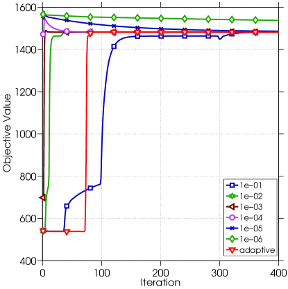
Figure 1: The evolution of the objective function value over time on instance case5, for a number of choices of $\mu$ and the adaptive updates of $\mu$.

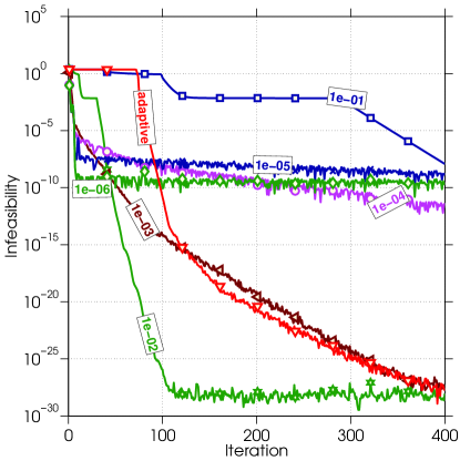
Figure 2: The evolution of the infeasibility over time on instance case5, for a number of choices of $\mu$ and the adaptive updates of $\mu$.

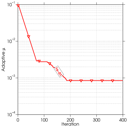
Figure 3: The evolution of $\mu$ with adaptive updates over time on instance case5.

7.5 Large Instances

We have also experimented with the so called Polish network [62], also known as case2224 and case2736sp, as well as the instances collected by the Pegase project [58], such as case9241peg. There, we cannot obtain solutions with the same precision as Matpower, within comparable run-times. However, we can decrease the initial infeasibility by factor of $10^{2}$ for case2224 in 200 seconds, by factor of $10^{6}$ for case2736sp in 200 seconds, and by factor of $10^{4}$ for case9241peg, again in 200 seconds. Although these results are not satisfactory, yet, they may be useful, when a good initial solution is available. As discussed in Section 8, we aim to improve upon these results by using a two-step method, where first-order methods on the convex problem are combined with a second-order method on the non-convex problem. These results also motivate the need for parallel computing.

7.6 Parallel Computing

As it has been discussed above, Algorithm 1 is easy to implement in a parallel fashion. We have implemented our multi-threading variant using OpenMP, in order to achieve portability. The significant overhead of using OpenMP makes it impossible to obtain a speed-up on very small instance. For example, in case3w, there is not enough work to be shared across (any number of) threads to offset the overhead. In Figure 4, we present the scaling properties of Algorithm 1. In particular, we illustrate the speed-up (the inverse of the multiple of single-threaded run-time) as a function of the number of cores used for a number of larger instances. We can also observe that even case118 is too small to benefit from a considerable speed-up. On the other hand, for large datasets, such as the Polish case2224 or larger, we observe a significant speed-up.

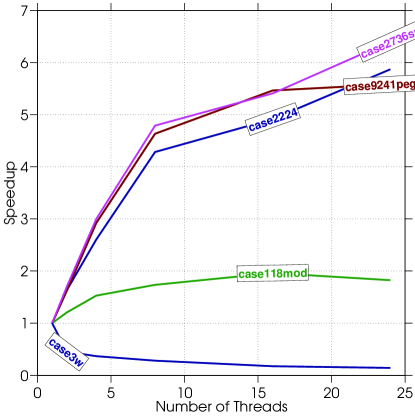
Figure 4: The speed-up as a function of the number of cores employed.

8 Conclusions

Our approach seems to bring the use of SDP relaxations of ACOPF closer to the engineering practice. A number of authors have recently explored elaborately constructed linear programming [5] and second-order cone programming [27, 42, 46, 24, 26] relaxations, many [27, 26] of which are not comparable to the SDP relaxations in the sense that they may be stronger or weaker, depending on the instance, but aiming to be solvable faster. Algorithm 1 suggests that there are simple first-order algorithms, which can solve SDP relaxations of ACOPF faster than previously, at least on some instances.

A major advantage of first-order methods over second-order methods [62, 55] is the ease of their parallelisability. This paper presents considers a symmetric multi-processing, where memory is shared, but a distributed variant, where ${\mathcal{C}}$ agents perform the iterations, is clearly possible, c.f. [41]. The ${\mathcal{C}}$ agents may represent companies, each of whom owns some of the generators and does not want to expose the details, such as cost functions. If ${\mathcal{C}}$ agents are ${\mathcal{C}}$ computers, a considerable speed-up can be obtained. Either way, power systems analysis could benefit from parallel and distributed computing.

The question as to how far could the method scale, remains open. In order to improve the scalability, one could try to combine first- and second-order methods [33]. We have experimented with an extension, which uses Smale’s $\alpha$-$\beta$ theory [6] to stop the computation at the point $z_{0}$, where we know, based on the analysis of the Lagrangian and its derivatives, that a Newton method or a similar algorithm with quadratic speed of convergence [14] will generate sequence $z_{i}$ to the correct optimum $z^{*}$, i.e.

$$|z_{i}-z^{*}|\leq(1/2)^{2^{i}-1}|z_{0}-z^{*}|.$$ (52)

This should be seen as convergence-preserving means of auto-tuning of the switch to a second-order method for convex functions.

One should also study infeasibility detection. Considering the test of feasibility of an SDP is not known to be in NP [53], we assumed the instance are feasible, throughout. Nevertheless, one may need to test their feasibility first, in many practical applications. There are some very fast heuristics [47] available already, but one could also use Lagrangian methods in a two-phase scheme, common in robust linear-programming solvers. Both in methods based on simplex and feasible interior-point, one first considers a variant of the problem, which has constraints relaxed by the addition of slack variables, with objective minimising a norm of the slack variables. This makes it possible to find feasible solutions quickly, and by duality, one can detect infeasibility.

One could also apply additional regularisations, following [34, 39]. In [R1], one could drop the rank-one constraint and modify the objective function to penalise the solutions with large ranks, e.g., by adding the term $\lambda\|W\|^{*}$ to the objective function, where $\|\cdot\|_{*}$ is a nuclear norm [18] and $\lambda>0$ is a parameter. Alternatively, one can replace the rank constraint by the requirement that the nuclear norm of the matrix should be small, i.e. $\|W\|_{*}\leq\lambda$. However, both approaches require a search for a suitable parameter $\lambda$ such that the optimal solution has indeed rank 1. Moreover, the penalised alternative may not produce an optimal solution of [PP4], necessitating further algorithmic work.

Finally, one could extend the method to solve relaxations a variety of related applications, such as security-constrained problems, stability-constrained problems, network expansion planning [40], and unit commitment problems. The question as to whether the method could generalise to the higher-order relaxations, c.f., Ghaddar et al. [19], also remains open. First steps [37] have been taken, but much work remains to be done.

References

- [1] E. Andersen, C. Roos, and T. Terlaky, On implementing a primal-dual interior-point method for conic quadratic optimization, Mathematical Programming 95 (2003), pp. 249–277.
- [2] X. Bai, H. Wei, K. Fujisawa, and Y. Wang, Semidefinite programming for optimal power flow problems, International Journal of Electrical Power & Energy Systems 30 (2008), pp. 383–392.
- [3] A.S. Bandeira, N. Boumal, and V. Voroninski, On the low-rank approach for semidefinite programs arising in synchronization and community detection, in Conference on Learning Theory (COLT), 2016., 2016.
- [4] A. Barvinok, A remark on the rank of positive semidefinite matrices subject to affine constraints, Discrete & Computational Geometry 25 (2001), pp. 23–31.
- [5] D. Bienstock and G. Munoz, LP approximations to mixed-integer polynomial optimization problems, CoRR abs/1501.00288 (2015).
- [6] L. Blum, F. Cucker, M. Shub, and S. Smale, Complexity and Real Computation, Springer-Verlag New York, Inc., Secaucus, NJ, USA, 1998.
- [7] B. Borchers, Csdp, ac library for semidefinite programming, Optimization methods and software 11 (1999), pp. 613–623.
- [8] N. Boumal, V. Voroninski, and A.S. Bandeira, The non-convex Burer-Monteiro approach works on smooth semidefinite programs, in Neural Information Processing Systems (NIPS 2016), 2016.
- [9] W.A. Bukhsh, A. Grothey, K.I. McKinnon, and P. Trodden, Local solutions of optimal power flow, IEEE Transactions on Power Systems 28 (2013), pp. 4780–4788.
- [10] S. Burer and C. Choi, Computational enhancements in low-rank semidefinite programming, Optimisation Methods and Software 21 (2006), pp. 493–512.
- [11] S. Burer and R.D. Monteiro, A nonlinear programming algorithm for solving semidefinite programs via low-rank factorization, Mathematical Programming 95 (2003), pp. 329–357.
- [12] S. Burer and R.D. Monteiro, Local minima and convergence in low-rank semidefinite programming, Mathematical Programming 103 (2005), pp. 427–444.
- [13] G. Cardano, Ars Magna Or The Rules of Algebra, Dover Books on Advanced Mathematics, Dover, a 1968 reprint of the 1545 original.
- [14] P. Chen, Approximate zeros of quadratically convergent algorithms, Mathematics of Computation 63 (1994), pp. 247–270.
- [15] C. Coffrin, D. Gordon, and P. Scott, NESTA, The NICTA Energy System Test Case Archive, ArXiv e-prints (2014).
- [16] A.R. Conn, N.I. Gould, and P. Toint, A globally convergent augmented lagrangian algorithm for optimization with general constraints and simple bounds, SIAM Journal on Numerical Analysis 28 (1991), pp. 545–572.
- [17] J. Czyzyk, M.P. Mesnier, and J.J. More, The neos server, IEEE Computational Science and Engineering 5 (1998), pp. 68–75.
- [18] M. Fazel, Matrix rank minimization with applications, Ph.D. diss., Stanford University, 2002.
- [19] B. Ghaddar, J. Marecek, and M. Mevissen, Optimal power flow as a polynomial optimization problem, IEEE Transactions on Power Systems 31 (2016), pp. 539–546.
- [20] L. Grippo, L. Palagi, and V. Piccialli, Necessary and sufficient global optimality conditions for nlp reformulations of linear sdp problems, Journal of Global Optimization 44 (2009), pp. 339–348.
- [21] C. Josz and D. Henrion, Strong duality in lasserre’s hierarchy for polynomial optimization, Optimization Letters 10 (2016), pp. 3–10.
- [22] C. Josz and D.K. Molzahn, Moment/sum-of-squares hierarchy for complex polynomial optimization, arXiv preprint arXiv:1508.02068 (2015).
- [23] C. Josz, J. Maeght, P. Panciatici, and J.C. Gilbert, Application of the moment-sos approach to global optimization of the opf problem, IEEE Transactions on Power Systems 30 (2015), pp. 463–470.
- [24] B. Kocuk, S.S. Dey, and X.A. Sun, New formulation and strong misocp relaxations for ac optimal transmission switching problem, arXiv preprint arXiv:1510.02064 (2015).
- [25] B. Kocuk, S.S. Dey, and X.A. Sun, Inexactness of sdp relaxation and valid inequalities for optimal power flow, IEEE Transactions on Power Systems 31 (2016), pp. 642–651.
- [26] B. Kocuk, S.S. Dey, and X.A. Sun, Strong socp relaxations for the optimal power flow problem, Operations Research (2016), p. to appear.
- [27] X. Kuang, L.F. Zuluaga, B. Ghaddar, and J. Naoum-Sawaya, Approximating the ACOPF problem with a hierarchy of SOCP problems, in Power Energy Society General Meeting, 2015 IEEE, July, 2015, pp. 1–5.
- [28] M. Laurent, Sums of squares, moment matrices and optimization over polynomials, in Emerging applications of algebraic geometry, Springer, 2009, pp. 157–270.
- [29] J. Lavaei and S. Low, Zero duality gap in optimal power flow problem, IEEE Transactions on Power Systems 27 (2012), pp. 92–107.
- [30] K. Lehmann, A. Grastien, and P.V. Hentenryck, Ac-feasibility on tree networks is np-hard, IEEE Transactions on Power Systems 31 (2016), pp. 798–801.
- [31] B. Lesieutre, D. Molzahn, A. Borden, and C. DeMarco, Examining the limits of the application of semidefinite programming to power flow problems, in Communication, Control, and Computing (Allerton), 2011 49th Annual Allerton Conference on, 2011, pp. 1492 –1499.
- [32] F. Li and R. Bo, Small test systems for power system economic studies, in Power and Energy Society General Meeting, 2010 IEEE, 2010, pp. 1–4.
- [33] A.C. Liddell, J. Liu, J. Marecek, and M. Takac, Hybrid methods in solving alternating-current optimal power flows, arXiv preprint arXiv:1510.02171 (2015).
- [34] R. Louca, P. Seiler, and E. Bitar, A rank minimization algorithm to enhance semidefinite relaxations of Optimal Power Flow, in Communication, Control, and Computing (Allerton), 2013 51st Annual Allerton Conference on, Oct, 2013, pp. 1010–1020.
- [35] S.H. Low, Convex relaxation of optimal power flow – part i: Formulations and equivalence, IEEE Transactions on Control of Network Systems 1 (2014), pp. 15–27.
- [36] S.H. Low, Convex relaxation of optimal power flow – part ii: Exactness, IEEE Transactions on Control of Network Systems 1 (2014), pp. 177–189.
- [37] W.J. Ma, Control, learning, and optimization for smart power grids, Ph.D. diss., The University of Notre Dame, 2015.
- [38] R. Madani, M. Ashraphijuo, and J. Lavaei, Promises of conic relaxation for contingency-constrained optimal power flow problem, IEEE Transactions on Power Systems 31 (2016), pp. 1297–1307.
- [39] R. Madani, J. Lavaei, and R. Baldick, Convexification of power flow problem over arbitrary networks, in 2015 54th IEEE Conference on Decision and Control (CDC), Dec, 2015, pp. 1–8.
- [40] J. Mareček, M. Mevissen, and J.C. Villumsen, MINLP in transmission expansion planning, in 2016 Power Systems Computation Conference (PSCC), June, 2016, pp. 1–8.
- [41] J. Mareček, P. Richtárik, and M. Takáč, Distributed block coordinate descent for minimizing partially separable functions, in Numerical Analysis and Optimization, Vol. 134, Springer, 2015, pp. 261–288.
- [42] D. Molzahn and I. Hiskens, Sparsity-exploiting moment-based relaxations of the optimal power flow problem, IEEE Transactions on Power Systems (2014).
- [43] D. Molzahn, B. Lesieutre, and C. DeMarco, A sufficient condition for global optimality of solutions to the optimal power flow problem, IEEE Transactions on Power Systems 29 (2014), pp. 978–979.
- [44] D. Molzahn, J. Holzer, B. Lesieutre, and C. DeMarco, Implementation of a large-scale optimal power flow solver based on semidefinite programming, IEEE Transactions on Power Systems 28 (2013), pp. 3987–3998.
- [45] D.K. Molzahn, Application of semidefinite optimization techniques to problems in electric power systems, Ph.D. diss., University of Wisconsin – Madison, 2013.
- [46] D.K. Molzahn and I.A. Hiskens, Mixed SDP/SOCP Moment Relaxations of the Optimal Power Flow Problem, in PowerTech Eindhoven 2015.
- [47] D.K. Molzahn, V. Dawar, B.C. Lesieutre, and C.L. DeMarco, Sufficient conditions for power flow insolvability considering reactive power limited generators with applications to voltage stability margins, in Bulk Power System Dynamics and Control - IX Optimization, Security and Control of the Emerging Power Grid (IREP), 2013 IREP Symposium, Aug, 2013, pp. 1–11.
- [48] K.G. Murty and S.N. Kabadi, Some np-complete problems in quadratic and nonlinear programming, Mathematical programming 39 (1987), pp. 117–129.
- [49] Y. Nesterov, Efficiency of coordinate descent methods on huge-scale optimization problems, SIAM Journal on Optimization 22 (2012), pp. 341–362.
- [50] G. Pataki, On the rank of extreme matrices in semidefinite programs and the multiplicity of optimal eigenvalues, Mathematics of operations research 23 (1998), pp. 339–358.
- [51] F. Permenter, H.A. Friberg, and E.D. Andersen, Solving conic optimization problems via self-dual embedding and facial reduction: a unified approach, Optimization Online (2015).
- [52] M.J. Powell, A fast algorithm for nonlinearly constrained optimization calculations, in Numerical analysis, Springer, 1978, pp. 144–157.
- [53] M. Ramana, An exact duality theory for semidefinite programming and its complexity implications, Mathematical Programming 77 (1997), pp. 129–162.
- [54] P. Richtárik and M. Takáč, Parallel coordinate descent methods for big data optimization, Mathematical Programming 156 (2016), pp. 433–484.
- [55] J.F. Sturm, Using sedumi 1.02, a matlab toolbox for optimization over symmetric cones, Optimization methods and software 11 (1999), pp. 625–653.
- [56] K.C. Toh, M.J. Todd, and R.H. Tütüncü, SDPT3 – A matlab software package for semidefinite programming, version 1.3, Optimization methods and software 11 (1999), pp. 545–581.
- [57] R.H. Tütüncü, K.C. Toh, and M.J. Todd, Solving semidefinite-quadratic-linear programs using SDPT3, Mathematical programming 95 (2003), pp. 189–217.
- [58] F. Villella, S. Leclerc, I. Erlich, and S. Rapoport, PEGASE pan-European test-beds for testing of algorithms on very large scale power systems, in Innovative Smart Grid Technologies (ISGT Europe), 2012 3rd IEEE PES International Conference and Exhibition on, Oct, 2012, pp. 1–9.
- [59] A. Wood and B. Wollenberg, Power Generation, Operation, and Control, A Wiley-Interscience publication, Wiley, 1996.
- [60] S. Wright, Coordinate descent algorithms, Mathematical Programming 151 (2015), pp. 3–34.
- [61] M. Yamashita, K. Fujisawa, M. Fukuda, K. Kobayashi, K. Nakata, and M. Nakata, Latest developments in the sdpa family for solving large-scale sdps, in Handbook on semidefinite, conic and polynomial optimization, Springer, 2012, pp. 687–713.
- [62] R.D. Zimmerman, C.E. Murillo-Sánchez, and R.J. Thomas, Matpower: Steady-state operations, planning and analysis tools for power systems research and education, IEEE Transactions on Power Systems 26 (2011), pp. 12–19.