Exact or approximate inference in graphical models: why the choice is dictated by the treewidth, and how variable elimination can be exploited

Abstract

Probabilistic graphical models offer a powerful framework to account for the dependence structure between variables, which is represented as a graph. However, the dependence between variables may render inference tasks intractable. In this paper we review techniques exploiting the graph structure for exact inference, borrowed from optimisation and computer science. They are built on the principle of variable elimination whose complexity is dictated in an intricate way by the order in which variables are eliminated. The so-called treewidth of the graph characterises this algorithmic complexity: low-treewidth graphs can be processed efficiently. The first message that we illustrate is therefore the idea that for inference in graphical model, the number of variables is not the limiting factor, and it is worth checking for the treewidth before turning to approximate methods. We show how algorithms providing an upper bound of the treewidth can be exploited to derive a ’good’ elimination order enabling to perform exact inference. The second message is that when the treewidth is too large, algorithms for approximate inference linked to the principle of variable elimination, such as loopy belief propagation and variational approaches, can lead to accurate results while being much less time consuming than Monte-Carlo approaches. We illustrate the techniques reviewed in this article on benchmarks of inference problems in genetic linkage analysis and computer vision, as well as on hidden variables restoration in coupled Hidden Markov Models.

Keywords: computational inference; marginalisation; mode evaluation; message passing; variational approximations.

1 Introduction

Graphical models  (Lauritzen, 1996; Bishop, 2006; Koller and Friedman, 2009; Barber, 2012; Murphy, 2012) are formed by variables linked to each other by stochastic relationships. They enable to model dependencies in possibly high-dimensional heterogeneous data and to capture uncertainty. Graphical models have been applied in a wide range of areas when elementary units locally interact with each other, like image analysis (Solomon and Breckon, 2011), speech recognition (Baker et al., 2009), bioinformatics (Liu et al., 2009; Maathuis et al., 2010; Höhna et al., 2014) and ecology (Illian et al., 2013; Bonneau et al., 2014; Carriger and Barron, 2016) to name a few.

In real applications a large number of random variables with a complex dependency structure are involved. As a consequence, inference tasks such as the calculation of a normalisation constant, of a marginal distribution or of the mode of the joint distribution can be challenging. Three main approaches exist to evaluate such quantities for a given distribution $\Pr$ defining a graphical model: $(a)$ compute them in an exact manner; $(b)$ use a stochastic algorithm to sample from the distribution $\Pr$ to get (unbiased) estimates; $(c)$ derive an approximation of $\Pr$ for which the exact calculation is possible. Even if appealing, exact computation on $\Pr$ can lead to very time and memory consuming procedures for large problems. The second approach is probably the most widely used by statisticians and modellers. Stochastic algorithms such as Monte-Carlo Markov Chains (MCMC) (Robert and Casella, 2004), Gibbs sampling (Geman and Geman, 1984; Casella and George, 1992) and particle filtering (Gordon et al., 1993) have become standard tools in many fields of application using statistical models. The last approach includes variational approximation techniques (Wainwright and Jordan, 2008), which are starting to become common practice in computational statistics. In essence, approaches of type $(b)$ provide an approximate answer to an exact problem whereas approaches of type $(c)$ provide an exact answer to an approximate problem.

In this paper, we focus on approaches of type $(a)$ and $(c)$, and we will review techniques for exact or approximate inference in graphical models borrowed from both optimisation and computer science. They are computationally efficient, yet not always standard in the statistician toolkit. The characterisation of the structure of the graph $G$ associated to a graphical model (precise definitions are given in Section 2) enables both to determine if the exact calculation of the quantities of interest (marginal distribution, normalisation constant, mode) can be implemented efficiently and to derive a class of operational algorithms. When the exact calculation cannot be achieved efficiently, a similar analysis of the problem enables the practitioner to design algorithms to compute an approximation of the desired quantities with an associated acceptable complexity. Our aim is to provide the reader with the key elements to understand the power of these tools for statistical inference in graphical models.

The central algorithmic tool we focus on in this paper is the variable elimination concept (Bertelé and Brioshi, 1972). In Section 3 we adopt a unified algebraic presentation of the different inference tasks (marginalisation, normalising constant or mode evaluation) to emphasise that each of them can be solved using a particular case of a variable elimination scheme. Consequently, the work done to demonstrate that variable elimination is efficient for one task passes on to the other ones. The key ingredient to design efficient algorithms based on variable elimination is the clever use of distributivity between algebraic operators. For instance distributivity of the product ($\times$) over the sum ($+$) enables to write $(a\times b)+(a\times c)=a\times(b+c)$ and evaluating the left-hand side of this equality requires two multiplications and one addition while evaluating the right-hand side requires one multiplication and one addition. Similarly since $\max(a+b,a+c)=a+\max(b,c)$ it is more efficient to compute the right-hand side from an algorithmic point of view. Distributivity enables to minimise the number of operations. To perform variable elimination, associativity and commutativity properties are also required, and the algebra behind is that of semi-ring (from which some notations will be borrowed). Inference algorithms using the distributivity property have been known and published in the Artificial Intelligence and Machine Learning literature under different names, such as sum-prod, or max-sum  (Pearl, 1988; Bishop, 2006). They are typical examples of variable elimination procedures.

Variable elimination relies on the choice of an order of elimination of the variables, via successive marginalisation or maximisation operations. The calculations are performed according to this ordering when applying distributivity. The topology of the graph $G$ provides key information to optimally organise the calculations as to minimise the number of elementary operations to perform. For example, when the graph is a tree, the most efficient elimination order corresponds to eliminating recursively the vertices of degree one. One starts from the leaves towards the root, and inner nodes of higher degree successively become leaves. The notion of an optimal elimination order for inference in an arbitrary graphical model is closely linked to the notion of treewidth of the associated graph $G$. We will see in Section 3 the reason why inference algorithms based on variable elimination with the best elimination order are of linear complexity in $n$, the number of variables/nodes in the graph, i.e. the size of the graph, but exponential complexity in the treewidth. Therefore treewidth is one the main characterisation of $G$ to determine if exact inference is possible in practice or not. This notion has lead to the development of several works for solving apparently complex inference problems, which have then been applied in biology (e.g. Tamura and Akutsu 2014). More details on these methodological and applied results are provided in the Conclusion Section.

The concept of treewidth has been proposed in parallel in computer science (Bodlaender, 1994), in discrete mathematics and graph minor theory (see Robertson and Seymour 1986; Lovász 2005). Discrete mathematics existence theorems (Robertson and Seymour, 1986) establish that there exists an algorithm for computing the treewidth of any graph with complexity polynomial in $n$ (but exponential in the treewidth), and the degree of the polynomial is determined. However, this result does not tell how to derive and implement the algorithm, apart from some very specific cases such as trees, chordal graphs, and series-parallel graphs (Duffin, 1965). Section 4 introduces the reader to several state-of-the-art algorithms that provide an upper bound of the treewidth, together with an associated elimination order. These algorithms are therefore useful tools to test if exact inference is achievable and, if applicable, to derive an exact inference algorithm based on variable elimination. Their behaviour is illustrated on benchmarks borrowed from combinatorial optimisation competitions.

Variable elimination also lead to message passing algorithms (Pearl, 1988) which are now common tools in computer science or machine learning for marginal or mode evaluation. More recently, these algorithms have been reinterpreted as a way to re-parameterise the original graphical model into an updated one with different potential functions by still representing the same join distribution  (Koller and Friedman, 2009). We explain in Section 5 how re-parametrisation can be used as a pre-processing tool to obtain a new parameterisation with which inference becomes simpler. Message passing is not the only way to perform re-parametrisation, and we discuss alternative efficient algorithms proposed in the context of Constraint Satisfaction Problems (CSP, see Rossi et al. 2006). These latter ones have, to the best of our knowledge, not yet been exploited in the context of graphical models.

As emphasised above, efficient exact inference algorithms can only be designed for graphical models with limited treewidth, i.e. much less than the number of vertices. Although this is not the case for many graphs, the principles of variable elimination and message passing for a tree can be applied to any graph leading to heuristic inference algorithms. The most famous heuristics is the Loopy Belief Propagation algorithm (LBP, see Kschischang et al. 2001). We recall in Section 6 the result that establishes LBP as a variational approximation method. Variational methods rely on the choice of a distribution which renders inference easier. They approximate the original complex graphical model. The approximate distribution is chosen within a class of models for which efficient inference algorithms exist, that is models with small treewidth (0, 1 or 2 in practice). We review some standard choices of approximate distributions, each of them corresponds to a different underlying treewidth.

Finally, Section 7 illustrates the techniques reviewed in the article, on the case of Coupled Hidden Markov Model (CHMM, see Brand 1997). We first compare them on the problem of mode inference in a CHMM devoted to the study of pest propagation. Then we exemplify the use of different variational methods for EM-based parameter estimation in CHMM.

2 Graphical Models

2.1 Models definition

Consider a stochastic system defined by a set of random variables $\mathbf{X}=(X_{1},\ldots,X_{n})^{\top}$. Each variable $X_{i}$ takes values in $\Lambda_{i}$. A realisation of $\mathbf{X}$ is denoted $\mathbf{x}=(x_{1},\ldots,x_{n})^{\top}$, with $x_{i}\in\Lambda_{i}$. The set of all possible realisations is called the state space, and is denoted $\Lambda=\prod_{i=1}^{n}\Lambda_{i}$. If $A$ is a subset of $V=\{1,\ldots,n\}$, then $X_{A}$, $x_{A}$ and $\Lambda_{A}$ are respectively the subset of random variables $\{X_{i},i\in A\}$, a possible realisation $\{x_{i},i\in A\}$ of $X_{A}$ and the state space of $X_{A}$ respectively. If $p$ is the joint probability distribution of ${\mathbf{X}}$ on $\Lambda$, we denote for all $\mathbf{x}\in\Lambda$

$$p(\mathbf{x})=\Pr(\mathbf{X}=\mathbf{x}).$$

Note that we focus here on discrete variables (we will discuss inference in the case of continuous variables on examples in Section 8). A joint distribution $p$ on $\Lambda$ is said to be a probabilistic graphical model (Lauritzen, 1996; Bishop, 2006; Koller and Friedman, 2009) indexed on a set $\mathcal{B}$ of parts of $V$ if there exists a set $\Psi=\{\psi_{B}\}_{B\in\mathcal{B}}$ of maps from $\Lambda_{B}$ to $\mathbb{R}^{+}$, called potential functions, indexed by $\mathcal{B}$ such that $p$ can be expressed in the following factorised form:

$$p({\mathbf{x}})=\frac{1}{Z}\prod_{B\in\mathcal{B}}\psi_{B}(x_{B}),$$ (1)

where $Z=\sum_{{\mathbf{x}}\in\Lambda}\prod_{B\in\mathcal{B}}\psi_{B}(x_{B})$ is the normalising constant, also called partition function. The elements $B\in\mathcal{B}$ are the scopes of the potential functions and $|B|$ is the arity of the potential function $\psi_{B}$. The set of scopes of all the potential functions involving variable $X_{i}$ is denoted $\mathcal{B}_{i}=\{B\in\mathcal{B}:i\in B\}$

One desirable property of graphical models is that of Markov local independence: if $p({\mathbf{x}})$ can be expressed as in (1), then a variable $X_{i}$ is (stochastically) independent of all others in ${\mathbf{X}}$ conditionally to the set of variables $X_{(\cup_{B\in\mathcal{B}_{i}}B)\setminus i}$. The set $X_{(\cup_{B\in\mathcal{B}_{i}}B)\setminus i}$is called the Markov blanket of $X_{i}$, or its neighbourhood (Koller and Friedman, 2009, chapter 4). It is denoted $N_{i}$. These conditional independences can be represented, by a graph with one vertex per variable in ${\mathbf{X}}$. The question of encoding the independence properties associated with a given distribution into a graph structure has been widely described (e.g. Koller and Friedman 2009, chapters 3 and 4), and we will not discuss it here. We consider the classical graph $G=(V,E)$ associated to the decomposition dictated in (1), where an edge is drawn between two vertices $i$ and $j$ if there exists $B\in\mathcal{B}$ such that $i$ and $j$ are in $B$. Such a representation of a graphical model is actually not as rich as the representation of (1). For instance, if $n=3$, the two cases $\mathcal{B}=\{\{1,2,3\}\}$ and $\mathcal{B}=\{\{1,2\},\{2,3\},\{3,1\}\}$ are represented by the same graph $G$, namely a clique (i.e. a fully connected set of vertices) of size 3. Without loss of generality, we could impose in the definition of a graphical model that scopes $B$ correspond to cliques of $G$. In the above example where $\mathcal{B}=\{\{1,2\},\{2,3\},\{3,1\}\}$, this can be done by defining $\psi^{\prime}_{1,2,3}=\psi_{12}\psi_{23}\psi_{13}$. The original structure is then lost, and $\psi^{\prime}$ is more costly to store than the original potential functions. The factor graph representation goes beyond the limit of the representation $G$: this graphical representation is a bipartite graph with one vertex per potential function and one vertex per variable. Edges are only between functions and variables. An edge is present between a function vertex (also called factor vertex) and a variable vertex, if and only if the variable is in the scope of the potential function. Figure 1 displays examples of the two graphical representations.

Several families of probabilistic graphical models exist (Koller and Friedman, 2009; Murphy, 2012). They can be grouped into directed and undirected ones. The most classical directed framework is that of Bayesian network (Pearl, 1988; Jensen and Nielsen, 2007). In a Bayesian network, potential functions are conditional probabilities of a variable given its parents. In such models, trivially $Z=1$. There is a representation by a directed graph where an edge is directed from a parent vertex to a child vertex (see Figure 1 (a)). The undirected graphical representation $G$ is obtained by moralisation, i.e. by adding an edge between two parents of a same variables. Undirected probabilistic graphical models (see Figure 1 (c)) are equivalent to Markov Random Fields (MRF, Li 2001) as soon as the potential functions take values in $\mathbb{R}^{+}\setminus\{0\}$. In a Markov random field (MRF), a potential function is not necessarily a probability distribution: $\psi_{B}$ is not required to be normalised (as opposed to a Bayesian network model).

Figure 1: From left to right: (a) Graphical representation of a directed graphical model where potential functions define the conditional probability of each variable given its parents values; (b) The corresponding factor graph where every potential function is represented as a factor (square vertex) connected to the variables that are involved in it; (c) Graphical representation of an undirected graphical model. It is impossible from this graph to distinguish between a graphical model defined by a unique potential function on vertices 3, 4 and 5 from a model defined by 3 pairwise potential functions over each pair $(3,4)$, $(3,5)$ and $(4,5)$; (d) The corresponding factor graph, which unambiguously defines the potential functions, here three pairwise potential functions.

Deterministic Graphical models.

Although the terminology of ’Graphical Models’ is often used to refer to probabilistic graphical models, the idea of describing a joint interaction on a set of variables through local functions has also been used in Artificial Intelligence to concisely describe Boolean functions or cost functions, with no normalisation constraint. Throughout this article we regularly refer to these deterministic graphical models, and we explain how the algorithms devoted to their optimisation can be directly applied to compute the mode in a probabilistic graphical model.

In a deterministic graphical model with only Boolean (0/1) potential functions, each potential function describes a constraint between variables. If the potential function takes value 1, the corresponding realisation is said to satisfy the constraint. If it takes value 0, the realisation does not satisfy it. The graphical model is known as a ’Constraint Network’. It describes a joint Boolean function on all variables that takes value 1 if and only if all constraints are satisfied. The problem of finding a realisation that satisfies all the constraints, called a solution of the constraint network, is the ’Constraint Satisfaction Problem’ (CSP, Rossi et al. 2006). This framework is used to model and solve combinatorial optimisation problems. There is a wide variety of software tools to solve it.

CSP have been extended to describe joint cost functions, decomposed as a sum of local cost functions, $f_{B}$ in the ‘Weighted Constraint Network’ (Rossi et al., 2006) or ‘Cost Function Network’.

$$f({\mathbf{x}})=\sum_{B\in\mathcal{B}}f_{B}(x_{B}).$$

In this case, cost functions take finite or infinite integer or rational values: infinity enables to express hard constraints while finite values encode costs for unsatisfied soft constraints. The problem of finding a realisation of minimum cost is the ’Weighted Constraint Satisfaction Problem’ (WCSP), which is NP-hard. It is easy to observe that any probabilistic graphical model can be translated in a weighted constraint network, and vice versa using a simple $-\ln(\cdot)$ transformation.

$$f_{B}(x_{B})=-\ln(\psi_{B}),\,\text{with }f_{B}(x_{B})=+\infty\Leftrightarrow\psi_{B}(x_{B})=0.$$

Therefore the WCSP is equivalent to finding a realisation with maximal probability in a probabilistic graphical model. With this equivalence, it becomes possible to use exact WCSP resolution algorithms that have been developed in this field for mode evaluation or for the computation of $Z$, the normalising constant, in probabilistic graphical model. See for instance Viricel et al. (2016), for an application on a problem of protein design.

2.2 Inference tasks in probabilistic graphical models

Computations on probabilities and potentials rely on two fundamental types of operations. Firstly, multiplication (or addition in the $\log$ domain) is used to combine potentials to define a joint potential distribution. Secondly, $\mathrm{sum}$ or $\max$/$\min$ can be used to eliminate variables and compute marginals or modes of the joint distribution on subsets of variables. The precise identity of these two basic operations is not important for the inference algorithms based on variable elimination. We therefore adopt a presentation using generic operators to emphasise this property of the algorithms. We denote as $\mathop{\odot}$ and as $\mathop{\oplus}$ the combination operator and the elimination operator, respectively. To be able to apply the variable elimination algorithm, the only requirement is that $(\mathbb{R}^{+},\mathop{\oplus},\mathop{\odot})$ defines a commutative semi-ring. Specifically, the semi-ring algebra offers distributivity: $(a\mathop{\odot}b)\mathop{\oplus}(a\mathop{\odot}c)=a\mathop{\odot}(b\mathop{\oplus}c)$. For instance, this corresponds to the distributivity of the product operation over the sum operation, i.e. $(a\times b)+(a\times c)=a\times(b+c)$, or to the distributivity of the $\max$ operation over the sum operation, i.e. $\max(a+b,a+c)=a+\max(b,c)$, or to the distributivity of the $\max$ operation over the product operation, i.e. $\max(a\times b,a\times c)=a\times(\max(b,c))$. We extend the definition of the two abstract operators $\mathop{\odot}$ and $\mathop{\oplus}$ to operators on potential functions, as follows:

Combine operator:

the combination of two potential functions $\psi_{A}$ and $\psi_{B}$ is a new function $\psi_{A}\mathop{\odot}\psi_{B}:\Lambda_{A\cup B}\to\mathbb{R}^{+}$ defined as $\psi_{A}\mathop{\odot}\psi_{B}(x_{A\cup B})=\psi_{A}(x_{A})\mathop{\odot}\psi_{B}(x_{B})$.

Elimination operator:

the elimination of variable $X_{i},i\in B$ from a potential function $\psi_{B}$ is a new function $(\mathop{\oplus}_{x_{i}}\psi_{B}):\Lambda_{B\setminus\{i\}}\to\mathbb{R}^{+}$ defined as $(\mathop{\oplus}_{x_{i}}\psi_{B})(x_{B\setminus\{i\}})=\mathop{\oplus}_{x_{i}}(\psi_{B}(x_{B\setminus\{i\}},x_{i}))$. For $\mathop{\oplus}=+$, $(\mathop{\oplus}_{x_{i}}\psi_{B})(x_{B\setminus\{i\}})$ represents the marginal sum $\sum_{x_{i}}\psi_{B}(x_{B\setminus\{i\}},x_{i})$.

Classical counting and optimisation tasks in graphical models can now be entirely written with these two operators. For simplicity, we denote by $\mathop{\oplus}_{x_{B}}$, where $B\subset V$ a sequence of eliminations $\mathop{\oplus}_{x_{i}}$ for all $i\in B$, the result being insensitive to the order in a commutative semi-ring. Similarly, $\mathop{\odot}_{B\in\mathcal{B}}$ represents the successive combination of all potential functions $\psi_{B}$, with $B\in\mathcal{B}$.

Counting task.

Under this name we group all tasks that involve summing over the state space of a subset of variables in ${\mathbf{X}}$. This includes the computation of the partition function $Z$ or of any marginal distribution, as well as entropy evaluation. For $A\subset V$ and $\bar{A}=V\setminus A$, the marginal distribution $p_{A}$ of $X_{A}$ associated to the joint distribution $p$ is defined as:

$$p_{A}(x_{A})=\sum_{x_{\bar{A}}\in\Lambda_{\bar{A}}}p\,(x_{A},x_{\bar{A}})=\frac{1}{Z}\sum_{x_{\bar{A}}\in\Lambda_{\bar{A}}}\prod_{B\in\mathcal{B}}\psi_{B}(x_{B})$$

The function $p_{A}$ then satisfies ($Z$ is a constant function):

$$p_{A}\mathop{\odot}Z=p_{A}\mathop{\odot}{\Big{(}\mathop{\mbox{\Large$\oplus$}}_{{\mathbf{x}}}\big{(}\mathop{\mbox{\Large$\odot$}}_{B\in\mathcal{B}}\psi_{B}\big{)}\Big{)}}=\Big{(}\mathop{\mbox{\Large$\oplus$}}_{x_{\bar{A}}}\big{(}\mathop{\mbox{\Large$\odot$}}_{B\in\mathcal{B}}\psi_{B}\big{)}\Big{)}$$

where $\mathop{\odot}$ combines functions using $\times$ and $\mathop{\oplus}$ eliminates variables using $+$.

Marginal evaluation is also interesting in the case where some variables are observed. If $x_{O}$ ($O\subset V$) are the values of the observed values, the marginal conditional distribution can be computed by restricting the domains of variables $X_{O}$ to the observed value. This is typically the kind of computational task required in the E-step of an EM algorithm, for parameter estimation of models with hidden data.

Optimisation task

The most common optimisation task in a graphical model corresponds to the evaluation of the most probable state ${\mathbf{x}}^{*}$ of the random vector ${\mathbf{X}}$, defined as

$${\mathbf{x}}^{*}=\arg\max_{{\mathbf{x}}\in\Lambda}p({\mathbf{x}})=\arg\max_{{\mathbf{x}}\in\Lambda}\prod_{B\in\mathcal{B}}\psi_{B}(x_{B})=\arg\max_{{\mathbf{x}}\in\Lambda}\sum_{B\in\mathcal{B}}\ln\psi_{B}(x_{B})$$

The maximum itself is $\mathop{\mbox{\Large$\oplus$}}_{{\mathbf{x}}}(\mathop{\mbox{\Large$\odot$}}_{B\in\mathcal{B}}\ln{\psi_{B}(x_{B})})$ with $\mathop{\oplus}$ and $\mathop{\odot}$ set to $\max$ and to $+$, respectively. The computation of the mode ${\mathbf{x}}^{*}$ does not require the computation of the normalising constant $Z$, however evaluating the mode probability value $p({\mathbf{x}}^{*})$ does. Another optimisation task of interest is the computation of the max-marginals of each variable $X_{i}$ defined as $p^{*}(x_{i})=\max_{x_{V\setminus i}}p({\mathbf{x}})$.

Therefore counting and optimisation tasks can be interpreted as two instantiations of the same computational task expressed in terms of combination and elimination operators, namely $\mathop{\mbox{\Large$\oplus$}}_{x_{A}}\mathop{\mbox{\Large$\odot$}}_{B\in\mathcal{B}}\psi_{B}$, where $A\subseteq V$. When the combination operator $\mathop{\odot}$ and the elimination operator $\mathop{\oplus}$ are set to $\times$ and $+$, respectively, this computational problem is known as a sum-product problem in the Artificial Intelligence literature (Pearl, 1988),(Bishop, 2006, chapter 8). When $\mathop{\oplus}$ and $\mathop{\odot}$ are set to $\max$ and to the sum operator, respectively it is a max-sum problem (Bishop, 2006, chapter 8). In practice, it means that tasks such as solving the E-step of the EM algorithm or computing the mode in a graphical model, belong to the same family of computational problems.

We will see in Section 3 that there exists an exact algorithm solving this general task which exploits the distributivity of the combination and elimination operators to perform operations in a smart order. From this generic algorithm, known as variable elimination (Bertelé and Brioshi, 1972) or bucket elimination (Dechter, 1999), one can deduce exact algorithms to solve counting and optimisation tasks in a graphical model, by instantiating the operators $\mathop{\oplus}$ and $\mathop{\odot}$.

Deterministic Graphical models.

The Constraint Satisfaction Problem is a $\lor$-$\land$ problem as it can can be defined using $\lor$ (logical ’or’) as the elimination operator and $\land$ (logical ’and’) as the combination operator over Booleans. The weighted CSP is a $\min$-$+$ as it uses $\min$ as the elimination operator and $+$ (or bounded variants of $+$) as the combination operator. Several other variants exist (Rossi et al., 2006), including generic algebraic variants (Schiex et al., 1995; Bistarelli et al., 1997; Cooper, 2004; Pralet et al., 2007; Kohlas, 2003).

Table 1: Definitions of the Combine ($\mathop{\odot}$) and the Elimination ($\mathop{\oplus}$) operators for classical tasks on probabilistic and deterministic graphical models.

Task	$\mathop{\oplus}$	$\mathop{\odot}$
Marginal evaluation	$+$	$\times$
Mode evaluation	$\max$	$+$
Existence of a solution in a CSP	$\lor$	$\land$
Evaluation of the minimum cost in WCSP	$\min$	$+$

2.3 Example: Coupled HMM

We introduce now the example of Coupled Hidden Markov Models (CHMM), which can be seen as extensions Hidden Markov Chain (HMC) models to several chains in interactions. In section 7 we will use this framework to illustrate the behaviour of exact and approximate algorithms based on variable elimination.

A HMC (Figure 2) is defined by two sequences of random variables ${\mathbf{O}}$ and ${\mathbf{H}}$ of same length, $T$. A realisation ${\mathbf{o}}=(o_{1},\ldots o_{T})^{\top}$ of the variables ${\mathbf{O}}=(O_{1},\ldots O_{T})^{\top}$ is observed, while the states of variables ${\mathbf{H}}=(H_{1},\ldots H_{T})^{\top}$ are unknown (hidden). In the HMC model the assumption is made that $O_{i}$ is independent of $H_{V\setminus\{i\}}$ and $O_{V\setminus\{i\}}$ given the hidden variable $H_{i}$. These independences are modelled by pairwise potential functions $\psi_{H_{i},O_{i}},\forall\ 1\leq i\leq T$. Furthermore, hidden variable $H_{i}$ is independent of $H_{1},\ldots,H_{i-2}$ and $O_{1},\ldots,O_{i-1}$ given the hidden variable $H_{i-1}$. These independences are modelled by pairwise potential functions $\psi_{H_{i-1},H_{i}},\forall\ 1<i\leq T$. Then the model is fully defined by specifying an additional potential function $\psi_{H_{1}}(h_{1})$ to model the initial distribution. In the classical HMC formulation (Rabiner, 1989), these potential functions are normalised conditional probability distributions i.e., $\psi_{H_{i-1},H_{i}}(h_{i-1},h_{i})=\Pr(H_{i}=h_{i}|H_{i-1}=h_{i-1})$, $\psi_{O_{i},H_{i}}(o_{i},h_{i})=\Pr(O_{i}=o_{i}|H_{i}=h_{i})$ and $\psi_{H_{1}}(h_{1})=\Pr(H_{1}=h_{1})$. As a consequence, the normalising constant $Z$ is equal to $1$, as it is in Bayesian networks.

Figure 2: Graphical representation of a HMM. Hidden variables correspond to vertices 1, 3, 5, 7, and observed variables to vertices 2, 4, 6, 8.

Consider now that there is more than one hidden chain: $I$ signals are observed at times $t\in\{1,\dots T\}$ and we denote $O^{i}_{t}$ the variable corresponding to the observed signal $i$ at time $t$. Variable $O^{i}_{t}$ depends on some hidden state $H^{i}_{t}$. The Coupled HMM (CHMM) framework assumes dependency between two hidden chains at two consecutive time steps (see Brand 1997): $H_{t}^{i}$ depends not only of $H_{t-1}^{i}$, it may depend on some $H_{t-1}^{j}$ for $j\neq i$. The set of the indices of chains upon which $H_{t}^{i}$ depends (expect $i$) is noted $L_{i}$. This results in the graphical structure displayed on Figure 3, where $L_{2}=\{1,3\}$ and $L_{1}=L_{3}=\{2\}$. Such models have been considered in a series of domains such as bioinformatics (Choi et al., 2013), electroencephalogram analysis (Zhong and Ghosh, 2002) or speech recognition (Nock and Ostendorf, 2003). In a CHMM setting, the joint distribution of the hidden variables ${\mathbf{H}}=(H^{i}_{t})_{i,t}$ and observed variables ${\mathbf{O}}=(O^{i}_{t})_{i,t}$ factorises as

$$\Pr({\mathbf{h}},{\mathbf{o}})\propto\prod_{i=1}^{I}\psi^{init}(h_{1}^{i})\left(\prod_{i=1}^{I}\prod_{t=2}^{T}\psi^{M}(h^{i}_{t-1},h_{t-1}^{L_{i}},h^{i}_{t})\right)\times\left(\prod_{i=1}^{I}\prod_{t=1}^{T}\psi^{E}(h^{i}_{t},o^{i}_{t})\right),$$ (2)

where $\psi^{init}$ is the initial distribution, $\psi^{M}$ encodes the local transition function of $H_{t}^{i}$ and $\psi^{E}$ encodes the emission of the observed signal given the corresponding hidden state. A fairly comprehensive exploration of these models can be found in (Murphy, 2002).

Figure 3: Graphical representation of a coupled HMM with 3 hidden chains.

Potential function $\psi^{init}$, $\psi^{M}$ and $\psi^{E}$ can be parameterised by a set of parameters denoted $\theta$. A classical problem for CHMM is have more than one iron in the fire: (a) estimate $\theta$ and (b) compute the mode of the conditional distribution of the hidden variables given the observations. Estimation can be performed using an EM algorithm, and as mentioned previously, the E-step of the algorithm and the mode computation task belong to the same family of computational task in graphical models. Both can be solved using variable elimination, as we show in the next section.

Beforehand, we present a reasonably simple example of CHMM that will be used to illustrate the different inference algorithms introduced in this work. It models the dynamics of a pest that can spread on a landscape composed of $I$ crop fields organised on a regular grid. The spatial neighbourhood of field $i$, denoted $L_{i}$, is the set of the four closest fields (three on the borders, and two in corners of the grid). $H_{t}^{i}\in\{0,1\}$ ($1\leq i\leq I,\ 1\leq t\leq T$) is the state of crop field $i$ at time $t$. State 0 (resp. 1) represents the absence (resp. presence) of the pest in the field. Variable $H_{t}^{i}$ depends on $H_{t-1}^{i}$ and of the $H_{t-1}^{j}$, for $j\in L_{i}$. The conditional probabilities of survival and apparition of the pest in field $i$ are parameterised by 3 parameters: $\epsilon$, the probability of contamination from outside the landscape (long-distance dispersal); $\rho$, the probability that the pest spreads from an infected field $j\in L_{i}$ to field $i$ between two consecutive times; and $\nu$, the probability of field persistent infection between two consecutive times. We assume that contamination events from all neighbouring fields are independent. Then, if ${C_{t}^{i}}$ is the number of contaminated neighbours of field $i$ at time $t$ (i.e. $C_{t}^{i}=\sum_{j\in L_{i}}H_{t}^{j}$), the contamination potential of field $i$ at time $t$ writes:

$$\psi^{M}(0,h_{t-1}^{L_{i}},1)=\Pr(H_{t}^{i}=1\mid H_{t-1}^{i}=0,h_{t-1}^{j},j\in L_{i})=\epsilon+(1-\epsilon)(1-(1-\rho)^{C_{t}^{i}}),$$

and its persistence in a contaminated state writes:

$$\psi^{M}(1,h_{t-1}^{L_{i}},1) = \Pr(H_{t}^{i}=1\mid h_{t-1}^{i}=1,h_{t}^{j},j\in L_{i})$$

$$= \nu+(1-\nu)\left(\epsilon+(1-\epsilon)(1-(1-\rho)^{C_{t}^{i}})\right).$$

The $(H_{t}^{i})$’s are hidden variables but monitoring observations are available. A binary variable $O_{t}^{i}$ is observed: it takes value 1, if the pest was declared as present in the field, and 0 otherwise. Errors of detection are possible. False negative observations occur since even if the pest is there, it can be difficult to notice, and missed. On the opposite, false positive observations occur when the pest is mixed up with another one. We define the corresponding emission potential as $\psi^{E}(0,1)=\Pr(O_{t}^{i}=0\mid H_{t}^{i}=1)=f_{n}$ and $\psi^{E}(1,0)=\Pr(O_{t}^{i}=1\mid H_{t}^{i}=0)=f_{p}$, respectively.

3 Variable elimination for exact inference

We describe now the principle of variable elimination to solve the general inference tasks presented in Section 2.2. We first recall the Viterbi algorithm for Hidden Markov Chains (Rabiner, 1989), a classical example of variable elimination for optimisation (mode evaluation). Then, we formally describe the variable elimination procedure in the general graphical model framework. The key element is the choice of an ordering for the sequential elimination of the variables. It is closely linked to the notion of treewidth of the graphical representation of the model. We explain how the complexity of a variable elimination algorithm is fully characterised by this notion. We also describe the extension to the elimination of blocks of variables.

3.1 Case of hidden Markov chain models

As a didactic introduction to exact inference on graphical models by variable elimination, we consider a well studied stochastic process: the discrete Hidden Markov Chain model (HMC).

A classical inference task for HMC is to identify the most likely values of variables ${\mathbf{H}}$ given a realisation ${\mathbf{o}}$ of the variables ${\mathbf{O}}$. The problem is to compute $\arg\max_{\mathbf{h}}\Pr({\mathbf{H}}={\mathbf{h}}|{\mathbf{O}}={\mathbf{o}})$, or equivalently the argument of:

$$\max_{h_{1},\ldots,h_{T}}\Big{[}(\psi_{H_{1}}(h_{1})\psi_{O_{1},H_{1}}(o_{1},h_{1}))\prod_{i=2}^{T}(\psi_{H_{i-1},H_{i}}(h_{i-1},h_{i})\psi_{O_{i},H_{i}}(o_{i},h_{i}))\Big{]}$$ (3)

The number of possible realisations of ${\mathbf{H}}$ is exponential in $T$. Nevertheless, this optimisation problem can be solved in a number of operations linear in $T$ using the well-known Viterbi algorithm (Rabiner, 1989). This algorithm, based on dynamic programming, performs successive eliminations (by maximisation) of all hidden variables, starting with $H_{T}$, and iteratively considering the $H_{i}$’s for $i=T-1,T-2,\ldots$, and finishing by $H_{1}$. It successively computes the most likely sequence of hidden variables. By using distributivity between the $\max$ and the product operators, the elimination of variable $H_{T}$ can be done by rewriting (3) as:

$$\max_{h_{1},\ldots,h_{T-1}}\Big{[}\psi_{H_{1}}(h_{1})\psi_{O_{1},H_{1}}(o_{1},h_{1})$$

$$\prod_{i=2}^{T-1}\big{(}\psi_{H_{i-1},H_{i}}(h_{i-1},h_{i})\psi_{O_{i},H_{i}}(o_{i},h_{i})\underbrace{\max_{h_{T}}\psi_{H_{T-1},H_{T}}(h_{T-1},h_{T})\psi_{O_{T},H_{T}}(o_{T},h_{T})}_{\textrm{\scriptsize New potential function}}\big{)}\Big{]}$$

The new potential function created by maximising on $H_{T}$ depends only on variable $H_{T-1}$. The same principle can then be applied to $H_{T-1}$ and so forth. This is a simple application of the general variable elimination algorithm that we describe in the next section.

3.2 General principle of variable elimination

In Section 2, we have seen that counting and optimisation tasks can be formalised by the same generic algebraic formulation

$$\mathop{\mbox{\Large$\oplus$}}_{x_{A}}(\mathop{\mbox{\Large$\odot$}}_{B\in\mathcal{B}}\psi_{B})$$ (4)

where $A\subseteq V$.

The trick behind variable elimination (Bertelé and Brioshi, 1972) relies on a clever use of the distributivity property. Indeed, evaluating $(a\mathop{\odot}b)\mathop{\oplus}(a\mathop{\odot}c)$ as $a\mathop{\odot}(b\mathop{\oplus}c)$ requires fewer operations. Hence eliminating $a$ in the second writing leads to dealing with fewer algebraic operations. Since distributivity applies both for counting and optimising tasks, variable elimination can be applied to both tasks. It also means that if variable elimination is efficient for one task it will also be efficient for the other one. As in the HMC example, the principle of the variable elimination algorithm for counting or optimising consists in eliminating variables one by one in an expression of the problem like in (4).

The elimination of the first variable, say $X_{i},i\in A$, is performed by merging all potential functions involving $X_{i}$ and applying operator $\mathop{\oplus}_{x_{i}}$ to these potential functions. Using commutativity and associativity of both operators, (4) can be rewritten as:

$$\mathop{\mbox{\Large$\oplus$}}_{x_{A}}(\mathop{\mbox{\Large$\odot$}}_{B\in\mathcal{B}}\psi_{B})=\mathop{\mbox{\Large$\oplus$}}_{x_{A\setminus\{i\}}}\mathop{\mbox{\Large$\oplus$}}_{x_{i}}\left((\mathop{\mbox{\Large$\odot$}}_{B\in\mathcal{B}\setminus\mathcal{B}_{i}}\psi_{B})\mathop{\mbox{\Large$\odot$}}(\mathop{\mbox{\Large$\odot$}}_{B\in\mathcal{B}_{i}}\psi_{B})\right),$$

where $\mathcal{B}_{i}$ is the subset of $V$ defined such as all its elements contain $i$. Then using distributivity of $\mathop{\odot}$ on $\mathop{\oplus}$, we obtain:

$$\mathop{\mbox{\Large$\oplus$}}_{x_{A}}(\mathop{\mbox{\Large$\odot$}}_{B\in\mathcal{B}}\psi_{B})=\mathop{\mbox{\Large$\oplus$}}_{x_{A\setminus\{i\}}}\Big{[}(\mathop{\mbox{\Large$\odot$}}_{B\in\mathcal{B}\setminus\mathcal{B}_{i}}\psi_{B})\mathop{\odot}\underbrace{(\mathop{\mbox{\Large$\oplus$}}_{x_{i}}\mathop{\mbox{\Large$\odot$}}_{B\in\mathcal{B}_{i}}\psi_{B})}_{\textrm{\scriptsize New potential function $\psi_{N_{i}}$}}\Big{]}$$

This shows that the elimination of $X_{i}$ results in a new graphical model, where variable $X_{i}$ and the potential functions $\psi_{B},B\in\mathcal{B}_{i}=\{B^{\prime},\>x_{i}\in B^{\prime}\}$ do not appear anymore. They are replaced by a new potential $\psi_{N_{i}}$ which does not involve $X_{i}$, but depends on its neighbours in $G$. The graph associated to the new graphical model is in a sense similar to the one of the original model. It is updated as follows: vertex $X_{i}$ is removed, and neighbours $X_{N_{i}}$ of $X_{i}$ are now connected together in a clique because they are all in the scope of $\psi_{N_{i}}$. The new edges between the neighbours of $X_{i}$ are called fill-in edges. For instance, when eliminating variable $X_{1}$ in the graph of Figure 4 (left), potential functions $\psi_{1,2},\ \psi_{1,3},\ \psi_{1,4}$ and $\psi_{1,5}$ are replaced by $\psi_{2,3,4,5}=\mathop{\oplus}_{x_{1}}(\psi_{1,2}\mathop{\odot}\psi_{1,3}\mathop{\odot}\psi_{1,4}\mathop{\odot}\psi_{1,4})$. The new graph is shown in Figure 4 (right).

Figure 4: Elimination of variable $X_{1}$ replaces the four pairwise potential functions involving variable $X_{1}$ with a new potential $\psi_{N_{1}}$, involving the four neighbours of vertex 1 in the original graph. The new edges created between these four vertices are called fill-in edges (dashed edges in the middle figure).

Interpretation for marginalisation, maximisation and finding the mode of a distribution

When the first elimination step is applied with $\mathop{\oplus}=+$ and $\mathop{\odot}=\times$, the probability distribution defined by this new graphical model is the marginal distribution $p_{V\setminus\{i\}}(x_{V\setminus\{i\}})$ of the original distribution $p$ (up to a constant). The complete elimination can be obtained by successively eliminating all variables in $X_{A}$. The result is a graphical model over $X_{V\setminus A}$, which specifies the marginal distribution $p_{V\setminus A}(x_{V\setminus A})$. When $A=V$, the result is a model with a single constant potential function with value $Z$.

If instead $\mathop{\oplus}$ is $\max$, and $\mathop{\odot}=\times$ (or $+$ with a log transformation of the potential functions) and $A=V$, the last potential function obtained after elimination of the last variable is equal to the maximum of the non-normalised distribution. So evaluating $Z$ or the maximal probability of a graphical model can be both obtained with the same variable elimination algorithm, just changing the definition of the $\mathop{\oplus}$ (and $\mathop{\odot}$ if needed) operator(s).
Lastly, if one is interested in the mode itself, an additional computation is required. The mode is actually obtained by induction: if $x^{*}_{V\setminus\{i\}}$ is the mode of the graphical model obtained after the elimination of the first variable, $X_{i}$, then the mode of $p$ can be defined as $(x^{*}_{V\setminus\{i\}},x^{*}_{i})$, where $x^{*}_{i}$ is a value in $\Lambda_{i}$ that maximises $\mathop{\odot}_{B\in\mathcal{B}}\psi_{B}(x^{*}_{V\setminus\{i\}},x_{i})$. This maximisation is straightforward to derive because $x_{i}$ can take only $|\Lambda_{i}|$ values. $x^{*}_{V\setminus\{i\}}$ itself is obtained by completing the mode of the graphical model obtained after elimination of the second variable, and so on. We stress here that the procedure requires to keep the intermediary potential functions $\psi_{N_{i}}$ created during the successive eliminations.

Complexity of the intermediary potential functions and variable elimination ordering: a prelude to the treewidth

When eliminating a variable $X_{i}$, the task which can be computationally expensive is the computation of the intermediate $\psi_{N_{i}}$. It requires to compute the product $\mathop{\odot}_{B\in\mathcal{B}_{i}}\psi_{B}(x_{B})$ of several potential functions for all elements of $\Lambda_{N_{i}\cup\{i\}}$, the state space of $X_{N_{i}\cup\{i\}}$. The time and space complexity of the operation are entirely determined by the cardinality $|N_{i}|$ of the set of indices in $N_{i}$. If $K=\max_{j\in V}|\Lambda_{j}|$, the time complexity (i.e. number of elementary operations performed) is in $O(K^{|N_{i}|+1})$ and space complexity (i.e. memory space needed) is in $O(K^{|N_{i}|})$. Complexity is therefore exponential in $|N_{i}|$, the number of neighbours of the eliminated variable in the current graphical model. The total complexity of the variable elimination is then exponential in the maximum cardinality $|N_{i}|$ over all successive eliminations. However note that it is linear in $n$, which means that a large $n$ is not necessarily a problem for having access to exact inference. Because the graphical model changes at each elimination step, this number usually depends on the order in which variables are eliminated.

As a consequence, the prerequisite to apply variable elimination is to decide for an ordering of the elimination of the variables. As illustrated in Figure 5 two different orders can lead to two different $N_{i}$ subsets. The key message is that the choice of the order is crucial. It dictates the efficiency of the variable elimination procedure. We now illustrate and formalise this intuition.

3.3 When is variable elimination efficient ?

We can understand why the Viterbi algorithm is an efficient algorithm for mode evaluation in a HMC. The graph associated to a HMC is comb-shaped: the hidden variables form a line and each observed variable is a leaf in the comb (see Figure 2). So it is possible to design an elimination order where the current variable to eliminate has a unique neighbour in the graphical representation of the current model: for instance $H_{T}>H_{T-1},\ldots>H_{1}$. By convention, the first eliminated variable is the largest according to this ordering (note that variables $O_{t}$ do not have to be eliminated since their value is known). Following this elimination order, when eliminating a variable using $\mathop{\oplus}$, the resulting graphical model has one fewer vertex than the previous one and no fill-in edge. Indeed, the new potential function $\psi_{N_{i}}$ is a function of a single variable since $|N_{i}|=1$. The Viterbi algorithm as a space complexity of $O(TK)$ and a time complexity of $O(TK^{2})$.

More generally, variable elimination is very efficient, i.e. leads to transitional $N_{i}$ sets of small cardinality, on graphical models whose graph representation is a tree. More specifically, for such graph structure, it is always possible to design an elimination order where the current variable to eliminate has only one neighbour in the graphical representation of the current model.

Another situation where variable elimination can be efficient is when the graph associated to the graphical model is chordal (any cycle of length four or more has a chord i.e., an edge connecting two non adjacent vertices in the cycle), and when the size of the largest clique is low. The rationale for this interesting property is explained intuitively here. In Figure 4, new edges are created between neighbours of the eliminated vertex. If this neighbourhood is a clique, no new edge is added. A vertex whose neighbourhood is a clique is called a simplicial vertex. Chordal graphs have the property that there exists an elimination order of the vertices, such that every vertex during the elimination process is simplicial (Habib and Limouzy, 2009). Consequently, there exists an elimination order such that no fill-in edges are created. Thus, the size of a transitional $N_{i}$’s is dictated by the size of the clique formed by the neighbours of $i$ Let us note that a tree is a chordal graph, in which all edges and only edges are cliques. Hence, for a tree, simplicial vertices are vertices of degree one. The elimination of degree one vertices on a tree is an example of simplicial elimination on a chordal graph.

For arbitrary graphs, if the maximal scope size of the intermediate $\psi_{N_{i}}$ functions created during variable elimination is too large, then memory and time required for the storage and computation quickly exceed computer capacities. Depending on the chosen elimination order, this maximal scope can be reasonable from a computational point of view, or too large. So again, the choice of the elimination order is crucial. In the case of CHMM, we can imagine two different elimination orders: either time slice per time slice, or chain by chain (we omit the observed variables that are known and do not have to be eliminated). For the first order, starting from the oriented graph of Figure 3, we first moralise it. Then, elimination of the variables $H_{T}^{i}$ of the last time step does not add any fill-in edges. However, when eliminating variables $H_{T-1}^{i}$ for $1\leq i\leq I-1$, due to the temporal dependences between chain, we create an intermediate potential function depending of $I+1$ variables ($H_{T-1}^{I}$ and the $H_{T-2}^{i}$ for all chains). And when successively eliminating temporal slices, the maximal size of the intermediate potential functions created is $I+1$. For the second elimination order, still starting from the moralised version of the oriented graph, after eliminating all variables $H_{t}^{1}$ for $1\leq t\leq T-1$, we create an intermediate potential function depending of $T+1$ variables ($H_{T}^{1}$ and $H_{t}^{2}$ for all $t$). And when successively eliminating chains, the maximal size of the intermediate potential functions created is $T+1$. So depending on the values of $I$ and $T$, we will not select the same elimination order.

3.4 The treewidth to characterise variable elimination complexity

The lowest complexity achievable when performing variable elimination is characterised by a parameter called the treewidth of the graph associated to the original graphical model. This concept has been repeatedly discovered and redefined. The treewidth of a graph is sometimes called its induced width (Dechter and Pearl, 1988), its minimum front size (Liu, 1992), its $k$-tree number (Arnborg, 1985), its dimension (Bertelé and Brioshi, 1972), and is also equal to the min-max clique number of $G$ minus one (Arnborg, 1985) to name a few. The treewidth is also a key notion in the theory of graph minors (Robertson and Seymour, 1986; Lovász, 2005).

We insist here on two definitions. The first one (Bodlaender, 1994) relies on the notion of induced graph (see Definition below). It highlights the close relationship between fill-in edges and the intermediate $N_{i}$ sets created during variable elimination. The second one (Robertson and Seymour, 1986; Bodlaender, 1994) is the most commonly used characterisation of the treewidth using so-called tree decompositions, also known as junction trees, which are key tools to derive variable elimination algorithms. It underlies the block-by-block elimination procedure described in Section 3.5.

Definition 1 (induced graph)

Let $G=(V,E)$ be a graph defined by a set of vertices indexed on $V$ and a set $E$ of edges. Given an ordering $\pi$ of the vertices of $G$, the induced graph $G^{ind}_{\pi}$ is defined in a constructive way as follows. First, $G$ and $G^{ind}_{\pi}$ have same vertices. Then for each edge in $E$ an oriented edge is added in $G^{ind}_{\pi}$ going from the first of the two nodes according to $\pi$ toward the second. Then each vertex $i$ of $V$ is considered one after the other following the order defined by $\pi$. When vertex $i$ is treated, an oriented edge is created between all pairs of neighbours of $i$ in $G$ that follow $i$ in the ordering defined by $\pi$. Again the edge is going from the first of the two nodes according to $\pi$ toward the second.

The induced graph $G^{ind}_{\pi}$ is also called the fill graph of $G$, and the process of computing it is sometimes referred to as “playing the elimination game” on $G$, as it just simulates elimination on $G$ using the variable ordering $\pi$ (see an example on Figure 5). This graph is chordal (Vandenberghe and Andersen, 2014). It is known that every chordal graph $G$ has at least one vertex ordering $\pi$ such that $G^{ind}_{\pi}=G$ (omitting the fact that edges of $G^{ind}_{\pi}$ are directed), called a perfect elimination ordering (Fulkerson and Gross, 1965).

Figure 5: A graph and two elimination orders. Left, the graph; middle, induced graph associated to the elimination order $(7>6>5>4>3>2>1)$. Vertices are eliminated from the largest to the smallest. The maximum size of $N_{i}$ sets created during elimination is $2$ (maximum number of outgoing edges) and only one (dashed) fill-in edge is added when vertex $4$ is eliminated; right, induced graph associated to the elimination order $(7>5>3>1>6>4>2)$. The maximum size of $N_{i}$ sets created during elimination is $3$ and 5 (dashed) fill-in edges are used.

The second notion that enables to define the treewidth is the notion of tree decomposition. Intuitively, a tree decomposition of a graph $G$ organises the vertices of $G$ in clusters of vertices which are linked by edges such that the graph obtained is a tree. Specific constraints on the way vertices of $G$ are associated to clusters in the decomposition tree are required. These constraints ensure that the resulting tree decomposition has properties useful for building variable elimination algorithms.

Definition 2 (tree decomposition)

Given a graph $G=(V,E)$, a tree decomposition of $G$, $T$, is a tree $(\mathcal{C},E_{T})$, where $\mathcal{C}=\{C_{1},\ldots,C_{l}\}$ is a family of subsets of $V$ (called clusters), and $E_{T}$ is a set of edges between the subsets $C_{i}$, satisfying the following properties:

• The union of all clusters $C_{k}$ equals $V$ (each vertex of $G$ is associated with at least one vertex of $T$).

• For every edge $(i,j)$ in $E$, there is at least one cluster $C_{k}$ that contains both $i$ and $j$.

• If clusters $C_{k}$ and $C_{l}$ both contain a vertex $i$ of $G$, then all clusters $C_{s}$ of $T$ in the (unique) path between $C_{k}$ and $C_{l}$ contain $i$ as well: clusters containing vertex $i$ form a connected subset of $T$. This is known as the running intersection property.

The concept of tree decomposition is illustrated in Figure 6.

Figure 6: Left: graphical representation of a graphical model. Right: tree decomposition over clusters $C_{1}=\{1,2,4\},\ C_{2}=\{1,3,4\},\ C_{3}=\{3,4,5\},\ C_{4}=\{5,6\}$ and $C_{5}=\{5,7\}$. Each edge between two clusters is labelled by their shared variables.

Definition 3 (treewidth)

The two following definitions of the treewidth derived respectively from the notion of induced graph, and from that of tree decomposition are equivalent:

• The treewidth ${\mathcal{T}W}_{\pi}(G)$ of a graph $G$ for the ordering $\pi$ is the maximum number of outgoing edges of a vertex in the induced graph $G^{ind}_{\pi}$. The treewidth ${\mathcal{T}W}(G)$ of a graph $G$ is the minimum treewidth over all possible orderings $\pi$.

• The width of a tree decomposition $(\mathcal{C},E_{T})$ is the size of the largest $C_{i}\in\mathcal{C}$ minus 1, and the treewidth ${\mathcal{T}W}(G)$ of a graph is the minimum width among all its tree decompositions.

It is not trivial to establish the equivalence (see Meseguer et al. 2006, chapter 7, and Schiex 1999). The term ${\mathcal{T}W}_{\pi}(G)$ is exactly the cardinality of the largest set $N_{i}$ created during variable elimination with elimination order $\pi$. For example, in Figure 5, the middle and right graphs are the two induced graphs for two different orderings and ${\mathcal{T}W}_{\pi}(G)$ is equal to 2 with the first ordering and to 3 with the second. It is easy to see that in this example ${\mathcal{T}W}(G)=2$. The treewidth of the graph of the HMC model, and of any tree is equal to 1.

It has been established that finding a minimum treewidth ordering $\pi$ for a graph $G$, finding a minimum treewidth tree decomposition, or computing the treewidth of a graph are of equivalent complexity. For an arbitrary graph, computing the treewidth is not an easy task. Section 4 is dedicated to this question, both from a theoretical and from a practical point of view.

The treewidth is therefore a key indicator to answer the driving subject of this review: will variable elimination be efficient for a given graphical model? For instance, the principle of variable elimination was applied to the exact computation of the normalising constant of a Markov random field on a small $r$ by $c$ lattice in Reeves and Pettitt (2004). For this regular graph, it is known that the treewidth is equal to $\min(r,c)$. So exact computation through variable elimination is possible for lattices with a small value for $\min(r,c)$ (even if $\max(r,c)$ is large). It is however well beyond computer capacities for real challenging problems in image analysis. In this case variable elimination can be used to define heuristic computational solutions, such as the algorithm of Friel et al. (2009), which relies on the merging of exact computations on small sub-lattices of the original lattice.

3.5 Tree decomposition and block by block elimination

Given a graphical model and a tree decomposition of its graph, a possible alternative to solve counting or optimisation tasks is to eliminate variables by successive blocks instead of one after the other. To do so, the block by block elimination procedure (Bertelé and Brioshi, 1972) relies on the tree decomposition characterisation of the treewidth. The underlying idea is to apply the variable elimination procedure on the tree decomposition, eliminating one cluster of the tree at each step. First a root cluster $C_{r}\in\mathcal{C}$ is chosen and used to define an order of elimination of the clusters, by progressing from the leaves toward the root. Every eliminated cluster corresponds to a leaf of the current intermediate tree. Then each potential function $\psi_{B}$ is assigned to the cluster $C_{i}$ in $\mathcal{C}$ such that $B\subset C_{i}$ which is the closest to the root. Such a cluster always exists otherwise either the running intersection property would not be satisfied or the graph of the decomposition would not be a tree. More precisely, the procedure starts with the elimination of any leaf cluster $C_{i}$ of $T$, with parent $C_{j}$ in $T$. Let us note $\mathcal{B}(C_{i})=\{B\in\mathcal{B},\psi_{B}\text{ assigned to }C_{i}\}$. Here again, commutativity and distributivity are used to rewrite expression (4) (with $A=V$) as follows:

$$\mathop{\mbox{\Large$\oplus$}}_{{\mathbf{x}}}\mathop{\mbox{\Large$\odot$}}_{B\in\mathcal{B}}\psi_{B}=\mathop{\mbox{\Large$\oplus$}}_{x_{V\setminus(C_{i}\setminus C_{j})}}\Big{[}\mathop{\mbox{\Large$\odot$}}_{B\in\mathcal{B}\setminus\mathcal{B}(C_{i})}\psi_{B}\mathop{\odot}\underbrace{(\mathop{\mbox{\Large$\oplus$}}_{x_{C_{i}\setminus C_{j}}}\mathop{\mbox{\Large$\odot$}}_{B\in\mathcal{B}(C_{i})}\psi_{B})}_{\textrm{\scriptsize New potential function}}\Big{]}$$

Note that only variables with indices in $C_{i}\setminus C_{j}\equiv C_{i}\cap(V\setminus C_{j})$ are eliminated, even if it is common to say that the cluster has been eliminated. For instance, in the example depicted in Figure 6, if the first eliminated cluster is $C_{1}$, the new potential function is $\mathop{\oplus}_{x_{2}}\psi_{1,2}(x_{1},x_{2})\psi_{2,4}(x_{2},x_{4})$, it depends only on variables $X_{1}$ and $X_{4}$. Cluster elimination continues until no cluster is left. The interest of this procedure is that the intermediate potential function created after each cluster elimination may have a scope much smaller than the treewidth, leading to better space complexity (Bertelé and Brioshi, 1972, chapter 4). However, the time complexity is increased.

In summary, the lowest achievable complexity when performing variable elimination is reached for elimination orders when the cardinality of the intermediate sets $N_{i}$ are smaller or equal to the treewidth of $G$. This treewidth can be determined by considering cluster sizes in tree decompositions of $G$. Furthermore, any tree decomposition $T$ can be used to build an elimination order and vice versa. Indeed, an elimination order can be defined by using a cluster elimination order based on $T$, and by choosing an arbitrary order to eliminate variables with indices in the subsets $C_{i}\setminus C_{j}$. Conversely, it is easy to build a tree decomposition from a given vertex ordering $\pi$. Since the induced graph $G^{ind}_{\pi}$ is chordal, its maximum cliques can be identified in polynomial time. Each such clique defines a cluster $C_{i}$ of the tree decomposition. Edges of $T$ can be identified as the edges of any minimum spanning tree in the graph with vertices $C_{i}$ and edges $(C_{i},C_{j})$ weighed by $|C_{i}\cap C_{j}|$.

Deterministic Graphical Models.

To our knowledge, the notion of treewidth and its properties were first identified in combinatorial optimisation in Bertelé and Brioshi (1972). It was then coined “dimension”, a graph parameter which was later shown to be equivalent to the treewidth (Bodlaender, 1998). Variable elimination itself is related to the Fourier-Motzkin elimination (Fourier, 1827), a variable elimination algorithm which benefits from the linearity of the handled formulas. Variable elimination has been repeatedly rediscovered, as non-serial dynamic programming (Bertelé and Brioshi, 1972), in the David-Putnam procedure for Boolean satisfiability problems (SAT, Davis and Putnam 1960), as Bucket elimination for the CSP and WCSP (Dechter, 1999), in the Viterbi and Forward-Backward algorithms for HMM (Rabiner, 1989) and many more.

There exists other situations where the choice of an elimination order has a deep impact on the complexity of the computations as in Gauss elimination scheme for a system of linear equations, or Choleski factorisation of very large sparse matrices, in which cases, the equivalence between elimination and decomposition was also used (see Bodlaender et al. 1995).

4 Treewidth approximation for exact inference

As already mentioned, the complexity of the counting and the optimisation tasks on graphical models is strongly linked to the treewidth ${\mathcal{T}W}(G)$ of the underlying graph $G$. If one could guess (one of) the optimal vertex ordering(s), $\pi^{*}$, leading to ${\mathcal{T}W}_{\pi^{*}}(G)={\mathcal{T}W}(G)$, then, one would be able to achieve the “optimal complexity” $O(K^{{\mathcal{T}W}(G)}n)$ for solving exactly these tasks; we recall that $K$ is the maximal domain size of a variable in the graphical model. However, the first obstacle to overcome is that the treewidth of a given graph cannot be evaluated easily: the treewidth computation problem is known to be NP-hard (Arnborg et al., 1987). If one has to spend more time on finding an optimal vertex ordering than on computing probabilities in the underlying graphical model, the utility of exact treewidth computation appears limited. Therefore, an alternative line of search is to look for algorithms computing a vertex ordering $\pi$ leading to a suboptimal width, ${\mathcal{T}W}_{\pi}(G)\geq{\mathcal{T}W}(G)$, but more efficient in terms of computational time. In the following, we describe and empirically compare heuristics which simultaneously provide a vertex ordering and an upper bound of the treewidth. Performing inference relying on this ordering is still exact. It is not optimal in terms of time complexity, but, on some problems, the inference can still be performed in reasonable time.

A broad class of heuristic approaches is that of greedy algorithms (Bodlaender and Koster, 2010). They use the same iterative approach as the variable elimination algorithm (Section 3) except that they only manipulate the graph structure. They do not perform any actual combination/elimination computation. Starting from an empty vertex ordering and an initial graph $G$, they repeatedly select the next vertex to add in the ordering by locally optimising one of the following criteria:

• select a vertex with minimum degree in the current graph ;

• select a vertex with minimum number of fill-in edges in the current graph.

After each vertex selection, the current graph is modified by removing the selected vertex and making a clique on its neighbours. The new edges added by this clique creation are fill-in edges. A vertex with no fill-in edges is a simplicial vertex (see Section 3.3). Fast implementations of minimum degree algorithms have been developed, see e.g., AMD (Amestoy et al., 1996) with time complexity in $O(nm)$ (Heggernes et al., 2001) for an input graph $G$ with $n$ vertices and $m$ edges. The minimum fill-in heuristics tend to be slower to compute but yield slightly better treewidth approximations in practice. Moreover, if a perfect elimination ordering (i.e., adding no fill-in edges) exists, this heuristic will find it. Thus, it recognises chordal graphs, and it returns the optimal treewidth in this particular case. This can be easily established from results in Bodlaender et al. 2005.

Notice that there exists linear time $O(n+m)$ algorithms to detect chordal graphs as the Maximum Cardinality Search (MCS) greedy algorithm (Tarjan and Yannakakis, 1984). MCS builds an elimination order based on the cardinality of the already processed neighbours. However, the treewidth approximation they return is usually worse than the previous heuristic approaches.

A simple way to improve the treewidth bound found by these greedy algorithms is to choose between candidate vertices with same value for the selected criterion by using a second criterion, such as minimum fill-in first and then maximum degree, or to choose at random and to iterate on the resulting randomised algorithms as done in Kask et al. (2011).

We compared the mean treewidth upper bound found by these four approaches (minimum degree, minimum fill-in, MCS and randomised iterative minimum fill-in) on a set of five WCSP and MRF benchmarks used as combinatorial optimisation problems in various solver competitions. ParityLearning is an optimisation variant of the minimal disagreement parity CSP problem originally contributed to the DIMACS benchmark and used in the Minizinc challenge (Optimization Research Group, 2012). Linkage is a genetic linkage analysis benchmark (Elidan and Globerson, 2010). GeomSurf and SceneDecomp are respectively geometric surface labelling and scene decomposition problems in computer vision (Andres et al., 2013). For each problem it is possible to vary the number of vertices and potential functions. The number of instances per problem as well as their mean characteristics are given in Table 2. Results are reported in Figure 7 (Left).The randomised iterative minimum fill-in algorithm used a maximum of $30,000$ iterations or $180$ seconds (respectively $10,000$ iterations and $60$ seconds for ParityLearning and Linkage), compared to a maximum of $0.37$ second used by the non-iterative approaches. The minimum fill-in algorithm (using maximum degree for breaking ties) performed better than the other greedy approaches. Its randomised iterative version offers slightly improved performance, at the price of some computation time.

Table 2: Characteristics of the five optimisation problems used as benchmark. For a given problem, several instances are available, corresponding to different numbers of variables (equal to the number of vertices in the underlying graph) and different numbers of potential functions.

Problem	Nb	Mean nb	Mean nb
Type/Name	of instances	of vertices	of potential functions
CSP/ParityLearning	7	659	1246
MRF/Linkage	22	917	1560
MRF/GeomSurf-3	300	505	2140
MRF/GeomSurf-7	300	505	2140
MRF/SceneDecomp	715	183	672

Then on the same benchmark, we compared three exact methods for the task of mode evaluation that exploit either minimum fill-in ordering or its randomised iterative version: variable elimination (ELIM), BTD (de Givry et al., 2006), and AND/OR Search (Marinescu and Dechter, 2006). Elim and BTD exploit the minimum fill-in ordering while AND/OR Search used its randomised iterative version. In addition, BTD and AND/OR Search exploit a tree decomposition during a Depth First Branch and Bound method in order to get a good trade-off between memory space and search effort. Just like variable elimination, they have a worst-case time complexity exponential in the treewidth. All methods were allocated a maximum of 1 hour and 4 GB of RAM on an AMD Operon 6176 at 2.3 GHz. The results are reported in Figure  7 (Right), and show that BTD was able to solve more problems than the two other methods for fixed CPU time. However, the best performing method heavily depends on the problem category. On ParityLearning, ELIM was the fastest method, but it ran out of memory on $83\%$ of the total set of instances, while BTD (resp. AND/OR Search) used less than $1.7$ GB (resp. 4GB). The randomised iterative minimum fill-in heuristic used by AND/OR Search in preprocessing consumed a fixed amount of time ($\approx 180$ seconds, included in the CPU time measurements) larger than the cost of a simple minimum fill-in heuristics run. BTD was faster than AND/OR Search to solve most of the instances except on two problem categories (ParityLearning and Linkage).

To perform this comparison, we ran the following implementation of each method. The version of ELIM was the one implemented in the combinatorial optimisation solver toolbar 2.3 (options -i -T3, available at mulcyber.toulouse.inra.fr/projects/toolbar). The version of BTD was the one implemented in the combinatorial optimisation solver toulbar2 0.9.7 (options -B=1 -O=-3 -nopre). Toulbar2 is available at www7.inra.fr/mia/T/toulbar2. This software won the UAI 2010 (Elidan and Globerson, 2010) and 2014 (Gogate, 2014) Inference Competitions on the MAP task. AND/OR Search was the version implemented in the open-source version 1.1.2 of daoopt (Otten et al., 2012) (options -y -i 35 --slsX=20 --slsT=10 --lds 1 -m 4000 -t 30000 --orderTime=180 for benchmarks from computer vision, and -y -i 25 --slsX=10 --slsT=6 --lds 1 -m 4000 -t 10000 --orderTime=60 for the other benchmarks) which won the Probabilistic Inference Challenge 2011 (Elidan and Globerson, 2011), albeit with a different closed-source version (Otten et al., 2012).

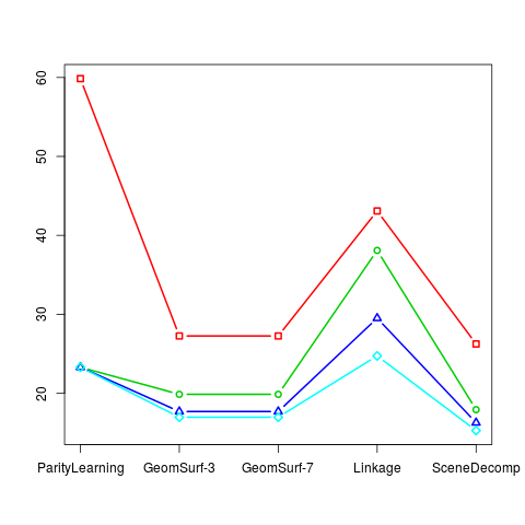
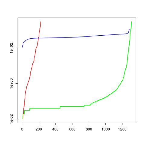
Figure 7: Left: Comparison of treewidth upper bounds provided by MCS (red), minimum degree (green), minimum fill-in (blue) and randomized iterative minimum fill-in (cyan) for the 5 categories of problems Right: Mode evaluation by three exact methods exploiting minimum fill-in ordering or its randomized iterative version. Number of instances solved ($x$-axis) within a given CPU time in seconds (log10 scale $y$-axis) of Elim (red), BTD (green), and AND/OR search (blue).

5 From Variable Elimination to Message Passing

On tree-structured graphical models, message passing algorithms extend the variable elimination algorithm by efficiently computing every marginals (or max-marginals) simultaneously, when variable elimination only computes one. On general graphical models, message passing algorithms can still be applied. They either provide approximate results efficiently, or have an exponential running cost.

We also present a less classical interpretation of the message passing algorithms: it may be conceptually interesting to view these algorithms as performing a re-parametrisation of the original graphical model, i.e. a rewriting of the potentials without modifying the joint distribution. Instead of producing external messages, the re-parametrisation produces an equivalent MRF, where marginals can be easily accessed, and which can be better adapted that the original one for initialising further processing.

5.1 Message passing and belief propagation

5.1.1 Message passing when the graph is a tree

Message passing algorithms over trees (Pearl, 1988) can be described as an extension of variable elimination, where the marginals or max-marginals of all variables are computed in a double pass of the algorithm. We depict the principle here when $G$ is a tree first and for marginal computation. At the beginning of the first pass (the forward pass) each leaf $X_{i}$ is marked as “processed“ and all other variables are ”unprocessed”. Then each leaf is successively visited and the new potential $\psi_{N_{i}}$ is considered as a “message” sent from $X_{i}$ to $X_{pa(i)}$ (the parents of $X_{i}$ in the tree), denoted as $\mu_{i\to pa(i)}$. This message is a potential function over $X_{pa(i)}$ only (scope of size 1). Messages are moved upward to nodes in the subgraph defined by unmarked variables. A variable is marked as processed once it has received its messages.

When only one variable remains unmarked (defining the root of the tree), the combination of all the functions on this variable (messages and possibly an original potential function involving only the root variable) will be equal to the marginal unnormalised distribution on this variable. This results directly from the fact that the operations performed in this forward pass of message passing are equivalent to variable elimination.

To compute the marginal of another variable, one can redirect the tree using this variable as a new root. Some subtrees will remain unchanged (in terms of direction from the root of the subtree to the leaves) in this new tree, and the messages in these subtrees do not need to be recomputed. The second pass (backward pass) of the message passing algorithm exploits the fact that messages are shared between several marginal computations, to organise all these computations in a clever way, so that in order to compute marginals of all variables, it is enough in the second pass to send messages from the root towards the leaf. Then the marginal is computed by combining downward messages with upward messages arriving at a particular vertex. One application is the well-known Forward-Backward algorithm (Rabiner, 1989).

Formally, in the message passing algorithm for marginal evaluation over a tree $(V,E)$, messages $\mu_{i\to j}$ are defined for each edge $(i,j)\in E$ in a leaves-to-root-to-leaves order; there are $2|E|$ such messages, one for each edge direction. Messages $\mu_{i\to j}$ are functions of $x_{j}$, which are computed iteratively, by the following algorithm:

1. First, messages leaving the leaves of the tree are computed: for each $i\in V$, where $i$ is a leaf of the tree, and for $j$ the unique parent of $i$, for all $(x_{i},x_{j})\in\Lambda_{i}\times\Lambda_{j}$:

   $$\mu_{i\to j}(x_{j})\leftarrow\sum_{x_{i}^{\prime}}\psi_{ij}(x_{i}^{\prime},x_{j})\psi_{i}(x_{i}^{\prime})$$

   Mark all leaves as processed.

2. Then, messages are sent upward through all edges. Message updates are performed iteratively, from marked nodes $i$ to their only unmarked neighbour $j$ through edge $(i,j)\in E$. Message updates take the following form for all $x_{j}\in\Lambda_{j}$:

   $$\mu_{i\to j}(x_{j})\leftarrow\frac{1}{K}\sum_{x_{i}^{\prime}}\psi_{ij}(x_{i}^{\prime},x_{j})\psi_{i}(x_{i}^{\prime})\prod_{k\neq j,(k,i)\in E}\mu_{k\to i}(x_{i}^{\prime}),$$ (5)

   where $K=\sum_{x_{j}}\sum_{x_{i}^{\prime}}\psi_{ij}(x_{i}^{\prime},x_{j})\psi_{i}(x_{i}^{\prime})\prod_{k\neq j,(k,i)\in E}\mu_{k\to i}(x_{i}^{\prime})$. In theory it is not necessary to normalise the messages, but this can be useful to avoid numerical problems.
   Mark node $j$ as processed. See Figure 8 for an illustration.

3. Send the messages downward (from root to leaves). This second phase of message updates takes the following form:

   • Unmark root node.

   • While there remains a marked node, send update (5) from an unmarked node to one of its marked neighbours, unmark the corresponding neighbour.

4. After the three above steps, messages have been transmitted through all edges in both directions. Finally, marginal distributions over variables and pairs of variables (linked by an edge) are computed as follows for all $(x_{i},x_{j})\in\Lambda_{i}\times\Lambda_{j}$:

   $$p_{i}(x_{i})\leftarrow\frac{1}{K_{i}}\psi_{i}(x_{i})\prod_{j,(j,i)\in E}\mu_{j\to i}(x_{i}),$$

   $$p_{ij}(x_{i},x_{j})\leftarrow\frac{1}{K_{ij}}\psi_{ij}(x_{i},x_{j})\prod_{k\neq j,(k,i)\in E}\mu_{k\to i}(x_{i})\prod_{l\neq i,(l,j)\in E}\mu_{l\to j}(x_{j})$$

   $K_{i}$ and $K_{ij}$ are suitable normalising constants.

Figure 8: Example of message update on a tree. In this example, nodes $t$, $v$ and $w$ are marked, while node $s$ is still unmarked. $\mu_{t\to s}$ is a function of all the incoming messages to node $t$, except $\mu_{s\to t}$.

Max-product and Max-sum algorithms can be equivalently defined on a tree, for exact computation of the $\max$-marginal of a joint distribution or its logarithm (see chapter 8 of Bishop 2006). In algebraic language, updates as defined by the formula of (5) take the general form:

$$\forall x_{j}\in\Lambda_{j},\mu_{i\to j}(x_{j})=\mathop{\oplus}_{x_{i}^{\prime}}\psi_{ij}(x_{i}^{\prime},x_{j})\psi_{i}(x_{i}^{\prime})\mathop{\odot}_{k\neq j,(k,i)\in E}\mu_{k\to i}(x_{i}^{\prime}).$$

5.1.2 Message passing when the factor graph is a tree

In some cases, the graph underlying the model may not be a tree, but the corresponding factor graph can be a tree, with factors potentially involving more than two variables (see Figure 9 for an example). In these cases, message passing algorithm can still be defined, and they lead to exact marginal value computations (or of max-marginals). However, their complexity becomes exponential in the size of the largest factor minus 1.

Figure 9: Left: Graphical model which structure is not a tree. Right: Corresponding factor graph, which is a tree. For applying message passing, the root is variable 1, while variables 4 and 5 are leaves. For the left branch the first messages sent is $\nu_{4\to\{2,4\}}(x_{4})$ followed by $\mu_{\{2,4\}\to 2}(x_{2})$

.

The message passing algorithm on a tree structured factor graph exploits the same idea of shared messages than in the case a tree structured graphical models, except that two different kinds of messages are computed:

• Factor-to-variable messages: messages from a factor $B$ (we identify the factor with the subset $B$ of the potential function $\psi_{B}$ it represents) towards a variable $i$, $\mu_{B\to i}(x_{i})$.

• Variable-to-factor messages: message from a variable $i$ towards a factor $B$, $\nu_{i\to B}(x_{i})$.

These are updated in a leaf-to-root direction and then backward, as above, but two different updating rules are used instead of (5): for all $x_{i}\in\Lambda_{i}$

$$\mu_{B\to i}(x_{i}) \leftarrow \sum_{x_{B\setminus i}}\left(\psi_{B}(x_{B})\prod_{j\in B\setminus i}\nu_{j\to B}(x_{j})\right),$$

$$\nu_{i\to B}(x_{i}) \leftarrow \prod_{B^{\prime}\neq B,i\in B^{\prime}}\mu_{B^{\prime}\to i}(x_{i}).$$

Then, the marginal probabilities are obtained by local marginalisation, as in Step 4 of the algorithm of Subsection 5.1.1 above.

$$p_{i}(x_{i})\leftarrow\frac{1}{K_{i}}\psi_{i}(x_{i})\prod_{B,i\in B}\mu_{B\to i}(x_{i}),\forall x_{i}\in\Lambda_{i},$$

where $K_{i}$ is again a normalising constant.

5.2 When the factor graph is not a tree

When the factor graph of the graphical model is not a tree, the two-pass message passing algorithm can no more be applied directly as is because of the loops. Yet, for general graphical models, this message passing approach can be generalised in two different ways.

• A tree decomposition can be computed, as previously discussed in Section 3.5. Message passing can then be applied on the resulting cluster tree, handling each cluster as a cross-product of variables following a block-by-block approach. This yields an exact algorithm, for which computations can be expensive (exponential in the treewidth) and space intensive (exponential in the separator size). A typical example of such algorithm is the algebraic exact message passing algorithm (Shafer and Shenoy, 1988; Shenoy and Shafer, 1990).

• Alternatively, the Loopy Belief Propagation algorithm (Frey and MacKay, 1998) is another extension of message passing in which messages updates are repeated, in arbitrary order through all edges (possibly many times through each edge), until a termination condition is met. The algorithm returns approximations of the marginal probabilities (over variables and pairs of variables). The quality of the approximation and the convergence to steady-state messages are not guaranteed, hence, the importance of the termination condition. However, it has been observed that LBP often provides good estimates of the marginals, in practice. A deeper analysis of the Loopy Belief Propagation algorithm is postponed to Section 6.

5.3 Message Passing and re-parametrisation

It is possible to use message passing as a re-parametrisation technique. In this case, the computed messages are directly used to reformulate the original graphical model in a new equivalent graphical model with the same graphical structure. By “equivalent” we mean that the potential functions are not the same but they define the same joint distribution as the original graphical model.

Several methods for re-parametrisation have been proposed both in the field of probabilistic graphical models (Koller and Friedman, 2009, chapters 10 and 13) or in the field of deterministic graphical models (Cooper et al., 2010). They all share the same advantage: the re-parameterised formulation can be computed to satisfy precise requirements. It can be designed so that the re-parameterised potential functions contains some information of interest (marginal distributions on singletons, on pairs $p_{i}(x_{i})$, max-marginals $p^{*}(x_{i})$, or their approximation). It can also be optimised in order to tighten a bound on the probability of a MAP assignment (Kolmogorov, 2006; Schiex, 2000; Cooper et al., 2010; Huang and Daphne Koller, 2013) or on the partition function (Wainwright et al., 2005; Liu and Ihler, 2011; Viricel et al., 2016). Originally naive bounds can be tightened into non-naive ones by re-parametrisation. An additional advantage of the re-parametrised distribution is in the context of incremental updates, where we have to perform inference based on the observation of some of the variables, and new observations (new evidence) are introduced incrementally. Since the the re-parameterised model already includes the result of previous inferences, it is more interesting (in term of number of message to send) to perform the updated inference when starting with this expression of the joint distribution that with the original one  (Koller and Friedman, 2009, chapter 10).

The idea behind re-parametrisation is conceptually very simple: when a message $\mu_{i\to j}$ is computed, instead of keeping it as a message, it is possible to combine any potential function involving $X_{j}$ with $\mu_{i\to j}$, using $\mathop{\odot}$. To preserve the joint distribution defined by the original graphical model, we need to divide another potential function involving $X_{j}$ by the same message $\mu_{i\to j}$ using the inverse of $\mathop{\odot}$.

Example for the computation of the max-marginals.

We illustrate here how re-parametrisation can be exploited to extract directly all (unnormalised) max-marginals $p^{*}(x_{i})$ from the order 1 potentials of the new model. In this case $\psi_{ij}$ is divided by $\mu_{i\to j}$, while $\psi_{j}$ is multiplied by $\mu_{i\to j}$. The same procedure can be run by replacing $\max$ by $+$ in the message definition to obtain all singleton marginals $P(x_{i})$ instead.

Let us consider a graphical model with 3 binary variables. The potential functions defining the graphical model are:

$$\psi_{1}(x_{1})=(3,1),\ \psi_{2}(x_{2}) = (2,6),\ \psi_{3}(x_{3})=(3,4)$$

$$\psi_{12}(x_{1},x_{2})=\left(\begin{array}[]{cc}3&2\\ 5&4\end{array}\right), \psi_{23}(x_{2},x_{3})=\left(\begin{array}[]{cc}4&8\\ 4&1\end{array}\right)$$ (10)

Since the graph of the model is a single path and is thus tree-structured, we just need two passes of messages. We use vertex 2 as the root. The first messages, from the leaves to the root, are:

$$\mu_{1\to 2}(x_{2}) = \max_{x_{1}}\psi_{1}(x_{1})\psi_{12}(x_{1},x_{2})$$

$$\mu_{3\to 2}(x_{2}) = \max_{x_{3}}\psi_{3}(x_{3})\psi_{23}(x_{2},x_{3})$$

We obtain

$$\mu_{1\to 2}(0)=\max(3\times 3,1\times 2)=9 \mu_{1\to 2}(1)=\max(3\times 2,1\times 4)=6$$ ,

$$\mu_{3\to 2}(0)=\max(3\times 4,4\times 8)=32 \mu_{3\to 2}(1)=\max(3\times 4,4\times 1)=12$$ ,

Potentials $\psi_{12}$ and $\psi_{23}$ are divided respectively by $\mu_{1\to 2}$ and $\mu_{3\to 2}$, while $\psi_{2}$ is multiplied by these two same messages. For instance

$$\psi^{\prime}_{2}(0) = \psi_{2}(0)\mu_{1\to 2}(0)\mu_{3\to 2}(0)=2\times 9\times 32=576$$

$$\psi^{\prime}_{2}(1) = \psi_{2}(1)\mu_{1\to 2}(1)\mu_{3\to 2}(1)=6\times 6\times 12=532$$

$$\psi^{\prime}_{12}(x_{1},0) = \frac{\psi_{12}(x_{1},0)}{\mu_{1\to 2}(0)},\ \psi^{\prime}_{12}(x_{1},1)=\frac{\psi_{12}(x_{1},1)}{\mu_{1\to 2}(1)}$$

All the updated potentials are:

$$\psi^{\prime}_{1}(x_{1})=\psi_{1}(x_{1})=(3,1),\ \psi^{\prime}_{2}(x_{2})=(576,432),\ \psi^{\prime}_{3}(x_{3})=\psi_{3}(x_{3})=(3,4)$$

$$\psi^{\prime}_{12}(x_{1},x_{2})=\left(\begin{array}[]{cc}3/9&2/6\\ 5/9&4/6\end{array}\right)=\left(\begin{array}[]{cc}1/3&1/3\\ 5/9&2/3\end{array}\right)$$ (15)

$$\psi^{\prime}_{23}(x_{2},x_{3})=\left(\begin{array}[]{cc}4/32&8/32\\ 4/12&1/12\end{array}\right)=\left(\begin{array}[]{cc}1/8&1/4\\ 1/4&1/12\end{array}\right)$$ (20)

Then messages from the root towards the leaves are computed using these updated potentials:

$$\mu_{2\to 1}(x_{1}) = \max_{x_{2}}\psi^{\prime}_{2}(x_{2})\psi^{\prime}_{12}(x_{1},x_{2})=(192,320)$$

$$\mu_{2\to 3}(x_{3}) = \max_{x_{2}}\psi^{\prime}_{2}(x_{2})\psi^{\prime}_{23}(x_{2},x_{3})=(144,144)$$

Finally, potentials $\psi^{\prime}_{12}$ and $\psi^{\prime}_{23}$ are divided respectively by $\mu_{2\to 1}$ and $\mu_{2\to 3}$, while $\psi^{\prime}_{1}$ and $\psi^{\prime}_{3}$ are multiplied by $\mu_{2\to 1}$ and $\mu_{2\to 3}$ respectively, leading to the re-parameterised potentials

$$\psi^{\prime\prime}_{1}(x_{1})=(3\times 192,1\times 320)=(576,320),\ \psi^{\prime\prime}_{2}(x_{2})=(576,432)$$

$$\psi^{\prime\prime}_{3}(x_{3})=(3\times 144,4\times 144)=(432,576)$$

$$\psi^{\prime\prime}_{12}(x_{1},x_{2})=\left(\begin{array}[]{cc}\frac{1}{3\times 192}&\frac{1}{3\times 192}\\ \frac{5}{9\times 320}&\frac{2}{3\times 320}\end{array}\right)=\left(\begin{array}[]{cc}\frac{1}{576}&\frac{1}{576}\\ \frac{1}{576}&\frac{1}{480}\end{array}\right)$$ (25)

$$\psi^{\prime\prime}_{23}(x_{2},x_{3})=\left(\begin{array}[]{cc}\frac{1}{8\times 144}&\frac{1}{4\times 144}\\ \frac{1}{3\times 144}&\frac{1}{12\times 144}\end{array}\right)=\left(\begin{array}[]{cc}\frac{1}{1152}&\frac{1}{576}\\ \frac{1}{432}&\frac{1}{1728}\end{array}\right)$$ (30)

Then we can directly read the (unnormalised) max marginal from the singleton potentials. For instance

$$\max_{x_{2},x_{3}}\psi_{1}(0)\psi_{2}(x_{2})\psi_{3}(x_{3})\psi_{12}(0,x_{2})\psi_{23}(x_{2},x_{3})=576=\psi^{\prime\prime}(0).$$

We can check that the original graphical model and the re- parameterised one define the same joint distribution by comparing to the (unnormalised) probability of each possible state (see Table 3).

Table 3: The unnormalised probabilities of the eight possible states in the original and re-parameterised models. One can check that the re-parameterised version describes the same joint distribution than the original one.

			Original		Reparameterised
$x_{1}$	$x_{2}$	$x_{3}$	$\psi_{1}\hfill\psi_{2}\hfill\psi_{3}\hfill\psi_{12}\hfill\psi_{23}\!$		$\psi^{\prime\prime}_{1}\hfill\psi^{\prime\prime}_{2}\hfill\psi^{\prime\prime}_{3}\hfill\psi^{\prime\prime}_{12}\hfill\psi^{\prime\prime}_{23}$
0	0	0	$3\times 2\times 3\times 3\times 4$	$=216=$	$576\times 576\times 432\times\frac{1}{576}\times\frac{1}{1152}$
0	0	1	$3\times 2\times 4\times 3\times 8$	$=576=$	$576\times 576\times 576\times\frac{1}{576}\times\frac{1}{576}$
0	1	0	$3\times 6\times 3\times 2\times 4$	$=432=$	$576\times 432\times 432\times\frac{1}{576}\times\frac{1}{432}$
0	1	1	$3\times 6\times 4\times 2\times 1$	$=144=$	$576\times 432\times 576\times\frac{1}{576}\times\frac{1}{1728}$
1	0	0	$1\times 2\times 3\times 5\times 4$	$=120=$	$320\times 576\times 432\times\frac{1}{576}\times\frac{1}{1152}$
1	0	1	$1\times 2\times 4\times 5\times 8$	$=320=$	$320\times 576\times 576\times\frac{1}{576}\times\frac{1}{576}$
1	1	0	$1\times 6\times 3\times 4\times 4$	$=288=$	$320\times 432\times 432\times\frac{1}{480}\times\frac{1}{432}$
1	1	1	$1\times 6\times 4\times 4\times 1$	$=96=$	$320\times 432\times 576\times\frac{1}{480}\times\frac{1}{1728}$

Re-parametrisation to compute pairwise or cluster joint distributions.

One possibility is to incorporate the messages in the binary potentials, in order to extract directly the pairwise joint distributions as described in Koller and Friedman (2009, chapter 10): $\psi_{ij}$ is replaced by $\psi_{ij}\mathop{\odot}\mu_{i\to j}\mathop{\odot}\mu_{j\to i}$ while $\psi_{i}$ is divided by $\mu_{j\to i}$ and $\psi_{j}$ by $\mu_{i\to j}$. If, for example, sum-prod messages are computed, each re-parameterised pairwise potential $\psi_{ij}$ can be shown to be equal to the (unnormalised) marginal distribution of $(X_{i},X_{j})$ (or an approximation of it if the graph is loopy).

In tree-structured problems, the resulting graphical model is said to be calibrated to emphasise the fact that all pairs of binary potentials sharing a common variable agree on the marginal distribution of this common variable (here $x_{i}$):

$$\mathop{\oplus}_{x_{j}}\psi_{ij}=\mathop{\oplus}_{x_{k}}\psi_{ik}$$

In the loopy case, if an exact approach using tree decomposition is followed, the domains of the messages have a size exponential in the size of the intersection of pairs of clusters, and the re-parametrisation will create new potentials of this size. These messages are included inside the clusters. Each resulting cluster potential will be the (unnormalised) marginal of the joint distribution on the cluster variables. Again, a re-parameterised graphical model on a tree-decomposition is calibrated, and any two intersecting clusters agree on their marginals. This is exploited in the Lauritzen-Spiegelhalter and Jensen sum-product-divide algorithms (Lauritzen and Spiegelhalter, 1988; Jensen et al., 1990). Besides its interest for incremental updates in this context, the re-parameterised graphical model using tree decomposition allows us to locally compute exact marginals for any set of variables in a same cluster.

If a local “loopy” approach is used instead, re-parameterisations do not change scopes, but provide a re-parameterised model. Estimates of the marginals of the original model can be read directly. For MAP, such re-parameterisations can follow clever update rules to provide convergent re-parameterisations maximising a well defined criterion. Typical examples of this process are the sequential version of the tree re-weighted algorithm (TRWS Kolmogorov 2006), or the Max-Product Linear Programming algorithm (MPLP, Globerson and Jaakkola 2008) which aims optimising a bound on the non-normalised probability of the mode. These algorithms can be exact on graphical models with loops, provided the potential functions are all submodular (often described as the discrete version of convexity, see for instance Topkis 1978; Cohen et al. 2004).

Re-parametrisation in deterministic graphical models.

Re-parameterising message passing algorithms have also been used in deterministic graphical models. They are then known as “local consistency” enforcing or constraint propagation algorithms. On one side, a local consistency property defines the targeted calibration property. On the other side, the enforcing algorithm uses so-called Equivalence Preserving Transformations to transform the original network into an equivalent network, i.e. defining the same joint function, which satisfies the desired calibration/local consistency property. Similar to LBP, Arc Consistency (Waltz, 1972; Rossi et al., 2006) is the most usual form of local consistency, and is related to Unit Propagation in SAT (Biere et al., 2009). Arc consistency is exact on trees, while it is usually incrementally maintained during an exact tree search, using re-parametrisation. Because of the idempotency of logical operators (they can be applied several time without changing the result obtained after the first application), local consistencies always converge to a unique fix-point.

Local consistency properties and algorithms for Weighted CSPs are closely related to message passing for MAP. They are however always convergent, thanks to suitable calibration properties (Schiex, 2000; Cooper and Schiex, 2004; Cooper et al., 2010), and also solve tree structured problems or problems where all potential functions are submodular.

These algorithms can be directly used to tackle the max-prod and sum-prod problems in a MRF. The re-parametrised MRF is then often more informative that the original one. For instance, under the simple conditions that all potential functions which scope larger than 1 are bounded by $1$, a trivial upper bound of the normalising constant $Z$ is $\prod_{i}\sum_{x_{i}}\psi_{i}(x_{i})$. This naive upper bound can be considerably tightened by re-parameterising the MRF using a soft-arc consistency algorithm (Viricel et al., 2016).

6 Heuristics and approximations for inference

We mainly discussed methods for exact inference in graphical models. They are useful if an order for variable elimination with small treewidth is available. In many real life applications, interaction network are seldom tree-shaped, and their treewidth can be large (e.g. a grid of pixel in image analysis). Consequently, exact methods cannot be applied anymore. However, they can be drawn inspiration from to derive heuristic methods for inference that can be applied to any graphical model. What is meant by a heuristic method is an algorithm that is (a priori) not derived from the optimisation of a particular criterion, the latter is rather termed an approximation method. Nevertheless, we shall alleviate this distinction, and show that good performing message passing-based heuristics can sometimes be interpreted as approximate methods. For the marginalisation task, the most widespread heuristics derived from variable elimination and message passing principles is the Loopy Belief Propagation In the last decade, a better understanding of these heuristics was reached, and they can now be re-interpreted as particular instances of variational approximation methods (Wainwright and Jordan, 2008). A variational approximation of a distribution $p$ is defined as the best approximation of $p$ in a class $\mathcal{Q}$ of tractable distributions (for inference), according to the Kullback-Leibler divergence. Depending of the application (e.g. discrete or continuous variables), several choices for $\mathcal{Q}$ can be considered. The connection with variable elimination principles and treewidth is not obvious at first sight. However, as we just emphasised, LBP can be cast in the variational framework. The treewidth of the chosen variational distribution depends on the nature of the variables: $i)$ in the case of discrete variables the treewidth need be low: in most cases, the class $\mathcal{Q}$ is formed by independent variables (mean field approximation), with associated treewidth equal to 0, and some works consider a class $\mathcal{Q}$ with associated treewidth equal to 1 (see Section 6.1); $ii)$ in the case of continuous variables, the treewidth of the variational distribution is the same as in the original model: $\mathcal{Q}$ is in general chosen to be the class of multivariate Gaussian distributions, for which numerous inference tools are available.

We recall here the two key components for a variational approximation method: the Kullback-Leibler divergence and the choice of a class of tractable distributions. We then explain how LBP can be interpreted as a variational approximation method. Finally we recall the rare examples where some statistical properties of an estimator obtained using a variational approximation have been established. In Section 7 we will illustrate how variational methods can be used to derive approximate EM algorithms for estimation in CHMM.

6.1 Variational approximations

The Kullback-Leibler divergence $KL(q||p)=\sum_{\mathbf{x}}q({\mathbf{x}})\log\frac{q({\mathbf{x}})}{p({\mathbf{x}})}$ measures the dissimilarity between two probability distributions $p$ and $q$. $KL$ is not symmetric, hence not a distance. It is positive, and it is null if and only if $p$ and $q$ are equal. Let us consider now that $q$ is constrained to belong to a family $\mathcal{Q}$, which does not include $p$. The solution $q^{*}$ of $\arg\min_{q\in\mathcal{Q}}KL(q||p)$ is then the best approximation of $p$ in $\mathcal{Q}$ according to the $KL$ divergence. It is called the variational distribution. If $\mathcal{Q}$ is a set of tractable distributions for inference, then marginals, mode or normalising constant of $q^{*}$ can be used as approximations of the same quantities on $p$.

Variational approximation were originally defined in the field of statistical mechanics, as approximations of the minimum of the free energy $F(q)$,

$$F(q)=-\sum_{\mathbf{x}}q({\mathbf{x}})\log\prod_{B\in\mathcal{B}}\psi_{B}(x_{B})+\sum_{\mathbf{x}}q({\mathbf{x}})\log q({\mathbf{x}}).$$

They are also known as Kikuchi approximations or Cluster Variational Methods (CVM, Kikuchi 1951). Minimising $F(q)$ is equivalent to minimising $KL(q||p)$, since

$$F(q)=-\sum_{\mathbf{x}}q({\mathbf{x}})\log p({\mathbf{x}})-\log(Z)+\sum_{\mathbf{x}}q({\mathbf{x}})\log q({\mathbf{x}})=KL(q||p)-\log(Z).$$

The mean field approximation is the most naive approximation among the family of Kikuchi approximations. Let us consider a binary Potts model on $n$ vertices whose joint distribution is

$$p({\mathbf{x}})=\frac{1}{Z}\prod_{i}\exp{(a_{i}x_{i}+\sum_{(i,j)\in E}b_{ij}x_{i}x_{j})}.$$

We can derive its mean field approximation, corresponding to the class $\mathcal{Q}^{MF}$ of fully factorised distributions (i.e. an associated graph of treewidth equal to 0): $\mathcal{Q}^{MF}=\{q,\text{ such that }q({\mathbf{x}})=\prod_{i\in V}q_{i}(x_{i})\}$.

Since variables are binary $\mathcal{Q}^{MF}$ corresponds to joint distributions of independent Bernoulli variables with respective parameters $q_{i}=_{def}q_{i}(1)$. Namely for all $q$ in $\mathcal{Q}^{MF}$, we can write $q({\mathbf{x}})=\prod_{i}q_{i}^{x_{i}}(1-q_{i})^{1-x_{i}}.$ The optimal approximation (in terms of Kullback-Leibler divergence) within this class of distributions is characterised by the set of $q_{i}$’s which minimise $KL(q||p)$. Denoting $E_{q}$ the expectation with respect to $q$, $KL(q||p)-\log Z$ is

$$E_{q}\left(\sum_{i}\left[X_{i}\log q_{i}+(1-X_{i})\log(1-q_{i})\right]-\sum_{i}a_{i}X_{i}-\sum_{(i,j)\in E}b_{ij}X_{i}X_{j}\right)$$

$$=\sum_{i}\left[q_{i}\log q_{i}+(1-q_{i})\log(1-q_{i})\right]-\sum_{i}a_{i}q_{i}-\sum_{(i,j)\in E}b_{ij}q_{i}q_{j}.$$

This expectation has a simple form because of the specific structure of $q$. Minimising it with respect to $q_{i}$ gives the fixed-point relation that each optimal $q_{i}^{MF}$’s must satisfy:

$$\log\left[{q_{i}^{MF}}/{(1-q_{i}^{MF})}\right]=a_{i}+\sum_{j:(i,j)\in E}b_{ij}q_{j}^{MF}.$$

leading to

$$q_{i}^{MF}=\frac{e^{a_{i}+\sum_{j:(i,j)\in E}b_{ij}q_{j}^{MF}}}{1+e^{a_{i}+\sum_{j:(i,j)\in E}b_{ij}q_{j}^{MF}}}.$$

It is interesting to note that this expression is very close to the expression of the conditional probability that $X_{i}=1$ given that all other variables in the neighbourhood of $i$:

$$\Pr(X_{i}=1\mid x_{N_{i}})=\frac{e^{a_{i}+\sum_{j:(i,j)\in E}b_{ij}x_{j}}}{1+e^{a_{i}+\sum_{j:(i,j)\in E}b_{ij}x_{j}}}.$$

The variational distribution $q_{i}^{MF}$ can be interpreted as equal to this conditional distribution, with neighbouring variables fixed to their expected values under distribution $q^{MF}$. It explains the name of mean field approximation. Note that in general $q_{i}$ is not equal to the marginal $p_{i}(1)$.

The choice of the class $\mathcal{Q}$ is indeed a critical trade-off between opposite desirable properties: it must be large enough to guarantee a good approximation, and small enough to contain only distributions for which inference in manageable. In the next section, a particular choice for $\mathcal{Q}$, the Bethe class, is emphasised. In particular, it enables us to link the LBP heuristics to variational methods. Other choices are possible, and have been used. For instance, in the structured mean field setting (Ghahramani and Jordan, 1997; Wainwright and Jordan, 2008), the distribution of a factorial Hidden Markov Model is approximated in a variational approach; the multivariate hidden state is decoupled, and the variational distribution $q$ of the conditional distribution of hidden states is that of independent Markov chains (here again, the treewidth is equal to 1). The Chow-Liu algorithm (Chow and Liu, 1968) computes the minimum of $KL(p||q)$ for a distribution $q$ whose associated graph is a spanning tree of the graph of $p$. This amounts to computing the best approximation of $p$ among graphical models with treewidth equal to 1. Finally, an alternative to treewidth reduction is to choose the variational approximation in the class of exponential distributions. This has been applied to Gaussian process classification (Kim and Ghahramani, 2006) using a multivariate Gaussian approximation of the posterior distribution of the hidden field. This method relies on the use of the EP algorithm (Minka, 2001). In this algorithm, $KL(p||q)$ is minimised instead of $KL(q||p)$. The choice of minimising one or the other depends on their computational tractability.

6.2 LBP heuristics as a variational method

If $p$ and $q$ are pairwise MRF whose associated graph $G=(V,E)$ is the same and is a tree, then $q({\mathbf{x}})=\frac{\prod_{(i,j)\in E}q(x_{i},x_{j})}{\prod_{i\in V}q(x_{i})^{d_{i}-1}}$, where $\{q(x_{i},x_{j})\}$ and $\{q(x_{i})\}$ are coherent sets of order 2 and order 1 marginals of $q$, respectively, and $d_{i}$ is the degree of vertex $i$ in the tree. In this particular case, the free energy is expressed as (see Heskes et al. 2004; Yedidia et al. 2005)

$$F(q) = -\sum_{(i,j)\in E}\sum_{x_{i},x_{j}}q(x_{i},x_{j})\log\psi(x_{i},x_{j})-\sum_{i\in V}\sum_{x_{i}}q(x_{i})\log\psi(x_{i})$$

$$+\sum_{(i,j)\in E}\sum_{x_{i},x_{j}}q(x_{i},x_{j})\log q(x_{i},x_{j})+\sum_{i\in V}(d_{i}–1)\sum_{x_{i}}q(x_{i})\log q(x_{i})$$

The Bethe approximation consists in applying to an arbitrary graphical model the same formula of the free energy as the one used for a tree, and then in minimising it over the variables $\{q(x_{i},x_{j})\}$ and $\{q(x_{i})\}$ under the constraint that they are probability distributions and that $q(x_{i})$ is the marginal of $q(x_{i},x_{j})$. By extension, the Bethe approximation can be interpreted as a variational method associated to the family $\mathcal{Q}^{Bethe}$ of unnormalised distributions that can be expressed as $q({\mathbf{x}})=\frac{\prod_{(i,j)\in E}q(x_{i},x_{j})}{\prod_{i\in V}q(x_{i})^{d_{i}-1}}$ with $\{q(x_{i},x_{j})\}$ and $\{q(x_{i})\}$ coherent sets of order 2 and order 1 marginals.

Yedidia et al. (2005) established that the fixed points of LBP (when they exist, convergence is still not well understood, see Weiss 2000 and Mooij and Kappen 2007) are stationary points of the problem of minimising the Bethe free energy, or equivalently $KL(q||p)$ with $q$ in the class $\mathcal{Q}^{Bethe}$ of distributions.

Furthermore, Yedidia et al. (2005) showed that for any class of distributions $\mathcal{Q}$ corresponding to a particular CVM method, it is possible to define a generalised BP algorithm whose fixed points are stationary points of the problem of minimising $KL(q||p)$ in $\mathcal{Q}$.

The drawback of the LBP algorithm and its extensions (Yedidia et al., 2005) is that they are not associated with any theoretical bound on the error made on the marginals approximations. Nevertheless, LBP is increasingly used for inference in graphical models for its good behaviour in practice  (Murphy et al., 1999). It is implemented in software packages for inference in graphical models like libDAI (Mooij, 2010) or OpenGM2 (Andres et al., 2012).

6.3 Statistical properties of variational estimates

Maximum-likelihood parameter estimation in graphical model is often intractable because it could require to compute marginals or normalising constants. A computationally efficient alternative to Monte-Carlo estimates are variational estimates, obtained using a variational approximation of the model. From a statistical point-of-view, because variational estimation is only an approximation of maximum-likelihood estimation, the resulting parameter estimates do not benefit of the typical properties of maximum-likelihood estimates (MLE), such as consistency or asymptotic normality. Unfortunately, no general theory exists for variational estimates, and results are available only for some specific models (see e.g. Hall et al. 2011 for the consistency in the Poisson log-normal model and Blei et al. 2017 for some other examples). From a more general point of view, in a Bayesian context, Wang and Titterington (2005) and Wang and Titterington (2006) studied the properties of variational estimates. They proved that the approximate conditional distribution are centred on the true posterior mean, but with a too small variance. Celisse et al. (2012) proved the consistency of the (frequentist) variational estimates of the Stochastic Block Model (SBM), while Gazal et al. (2012) empirically established the accuracy of their Bayesian counterpart. Variational Bayes estimates are also proposed by Jaakkola and Jordan (2000) for logistic regression, and the approximate posterior also turns out to be very accurate. A heuristic explanation for these two positive examples (SBM and logistic regression) is that, in both cases, the class $\mathcal{Q}$ used for the approximate conditional (or posterior) distribution $q$ is sought so as to asymptotically contain the true conditional distribution.

7 Illustration on CHMM

In this last section, we illustrate how the different discussed algorithms, in the CHMM framework, perform in practice for marginal inference when the model parameters are known, and how concretely they can be exploited in the EM algorithm to perform parameter estimation.

7.1 Comparison of exact variable elimination, variational inference and Gibbs sampling in practice

We compared the following inference algorithms on the problem of computing the marginals of all the hidden variables of the CHMM model of pest propagation described in Section 2.3, conditionally to the observed variables. We simulated 10 datasets with the following parameters values: $\rho=0.2,\nu=0.5,\epsilon=0.15,f_{n}=0.3$ and $f_{p}=0.1$. For each data set, we ran the following algorithms, using libDAI software (Mooij, 2010): junction tree (JT, exact method using the principles of tree decomposition and block by block elimination); loopy belief propagation (LBP); mean field approximation (MF); and Gibbs sampling (GS, Geman and Geman 1984), with 10,000 runs, each with a burn-in of 100 iterations and then 10,000 iterations. We compared the algorithms on three criteria: running time (time variable), mean absolute difference between the true marginal probability of state 0 and the estimated one, over all hidden variables (diff-marg variable), and percentage of hidden variables which are not restored to their true value with the mode of the estimated marginal (error-resto variable). The results (see Table 4) are presented for increasing values of $n$, the number of rows (and also of columns) of the square grid of fields (i.e. $I=n^{2}$). Beyond $n=3$, JT cannot be run, so for computing diff-marg we used the GS marginals instead of the true marginals. These results illustrate well the fact that approximate inference methods based on the principle of variable elimination are very time efficient compared to Monte-Carlo methods (less than 4 minutes for a problem with $I=10,000$ hidden variables), while being still very accurate. Furthermore, even a naive variational method like the mean field one can be interesting if accurate marginal estimates are not required but we are only interested in preserving their mode.

Table 4: Comparison of Junction Tree (JT), Loopy Belief Propagation (LBP), Mean Field (MF) and Gibbs sampling (GS) inference algorithms on the CHMM model of pest propagation: (a) running time, in second; (b) mean difference between the true and the estimated marginal of state 0 (when JT cannot be ran we use GS marginals as true ones); (c) percentage of hidden variables not restored to their true value when using the mode of the marginals.

time JT LBP MF GIBBS $n=3$ $0.04$ $0.04$ $0.03$ $1.05$ $n=5$ $-$ $0.19$ $0.14$ $3.30$ $n=10$ $-$ $1.07$ $0.65$ $13.99$ $n=100$ $-$ $219.31$ $134.31$ $3,499.6$ $n=200$ $-$ $1,026.2$ $746.68$ $29,341.0$	diff-marg LBP MF GIBBS $n=3$ $0.001$ $0.032$ $0.032$ $n=5$ $0.003$ $0.037$ $-$ $n=10$ $0.003$ $0.032$ $-$ $n=100$ $0.003$ $0.032$ $-$ $n=200$ $0.003$ $0.032$ $-$
(a)	(b)

error-resto	JT	LBP	MF	GIBBS
$n=3$	$20.00$	$19.80$	$19.26$	$20.19$
$n=5$	$-$	$18.60$	$19.27$	$18.93$
$n=10$	$-$	$17.87$	$17.70$	$17.83$
$n=100$	$-$	$18.19$	$18.39$	$18.20$
$n=200$	$-$	$18.18$	$18.40$	$18.18$
		(c)

7.2 Variational approximation for estimation in CHMM

We now illustrate how variational approximations have been used for parameter estimation using an EM algorithm in the case of CHMM.

Exact EM algorithm

CHMM are examples of incomplete data models, as they involve variables $({\mathbf{O}},{\mathbf{H}})$, and only variables ${\mathbf{O}}$ are observed. Maximum likelihood inference for such a model aims at finding the value of the parameters $\theta$ which maximise the (log-)likelihood of the observed data ${\mathbf{o}}$, i.e. to solve $\max_{\theta}\log\Pr^{\theta}({\mathbf{o}})$. The most popular algorithm to achieve this task is the EM algorithm (Dempster et al., 1977). One of its formulation reads as an iterative maximisation procedure of the following functional:

$$F(\theta,q)=E_{q}(\log{\Pr}^{\theta}({\mathbf{o}},{\mathbf{H}}))-E_{q}(\log q({\mathbf{H}}))=\log{\Pr}^{\theta}({\mathbf{o}})-KL(q({\mathbf{H}})||{\Pr}^{\theta}({\mathbf{H}}|{\mathbf{o}})),$$

where $q$ stands for any distribution on the hidden variables ${\mathbf{H}}$, and $E_{q}$ stands for the expectation under the arbitrary distribution $q$. The EM algorithm consists in alternatively maximising $F(\theta,q)$ with respect to $q$ (E-step) and to $\theta$ (M-step). The solution of the E-step is $q({\mathbf{h}})={\Pr}^{\theta}({\mathbf{h}}|{\mathbf{o}})$, since the Kullback-Leibler divergence is then minimal, and even null in this case. When replacing $q({\mathbf{h}})$ by $q({\mathbf{h}})={\Pr}^{\theta}({\mathbf{h}}|{\mathbf{o}})$ in $F$, we obtain that the M-step amounts to maximising $E\left[\log{\Pr}^{\theta}({\mathbf{o}},{\mathbf{H}})|{\mathbf{o}}\right]$.

Exact computation of ${\Pr}^{\theta}({\mathbf{h}}|{\mathbf{o}})$ can be performed by observing that (2) can be rewritten as

$${\Pr}^{\theta}({\mathbf{h}},{\mathbf{o}})\propto\psi^{init^{\prime}}(h_{1})\left(\prod_{t=2}^{T}\psi^{M^{\prime}}(h_{t-1},h_{t})\right)\times\left(\prod_{i=1}^{I}\prod_{t=1}^{T}\psi^{E}(h^{i}_{t},o^{i}_{t})\right),$$

where $\psi^{init^{\prime}}$ is the global initial distribution, equal to $\prod_{i=1}^{I}\psi^{init}(h_{1}^{i})$, and $\Psi^{M^{\prime}}$ is the global transition probability, equal to $\prod_{i=1}^{I}\psi^{M}(h_{t-1}^{i},h_{t-1}^{L-i},h_{t}^{i})$. This writing is equivalent to merging all hidden variables of a given time step. It corresponds to the graphical model given in Figure 10. Denoting $K$ the number of possible values for each hidden variables, we end up with a regular hidden Markov model with $K^{I}$ possible hidden states. Both ${\Pr}^{\theta}({\mathbf{h}}|{\mathbf{o}})$ and its mode can then be computed in an exact manner with either the forward-backward recursion or the Viterbi algorithm for the mode evaluation. Both procedures have the same complexity: $O(TK^{2I})$. The exact calculation can therefore be achieved provided that $K^{I}$ remains small enough, but becomes intractable when the number of signals $I$ exceeds a few tens.

Figure 10: Graphical representation of $\Pr({\mathbf{h}},{\mathbf{o}})$ for a coupled HMM when merging hidden variables at each time step

Several variational approximations for the EM algorithm

For more complex graphical structure, explicitly determining ${\Pr}^{\theta}({\mathbf{h}}|{\mathbf{o}})$ can be too expensive to perform exactly. A first approach to derive an approximate E-step is to seek for a variational approximation of ${\Pr}^{\theta}({\mathbf{h}}|{\mathbf{o}})$ assuming that $q({\mathbf{h}})$ is restricted to a family $\mathcal{Q}$ of tractable distributions, as described in Section 6.1. The choice of $\mathcal{Q}$ is critical, and requires achieving an acceptable balance between approximation accuracy and computation efficiency. Choosing $\mathcal{Q}$ typically amounts to breaking down some dependencies in the original distribution to end up with some tractable distribution. In the case of CHMM, the simplest distribution is the class of fully factorised distributions (i.e. mean field approximation), that is

$$\mathcal{Q}_{0}=\{q:q({\mathbf{h}})=\prod_{i=1}^{I}\prod_{t=1}^{T}q_{it}(h^{i}_{t})\}.$$

Such an approximation of ${\Pr}^{\theta}({\mathbf{h}}|{\mathbf{o}})$ corresponds to the graphical model of Figure 11. Intuitively, this approximation replaces the stochastic influence between the hidden variables by its mean value.

Figure 11: Graphical representation for the mean-field approximation of $\Pr({\mathbf{h}},{\mathbf{o}})$ in a coupled HMM. Observed variables are indicated in light grey since they are not part of the variational distribution which is a distribution only on the hidden variables.

As suggested in Wainwright and Jordan (2008), a less drastic approximation of ${\Pr}^{\theta}({\mathbf{h}}|{\mathbf{o}})$ can be obtained using the distribution family of independent heterogeneous Markov chains:

$$\mathcal{Q}_{M}=\{q:q({\mathbf{h}})=\prod_{i}\prod_{t}q_{it}(h^{i}_{t}|h^{i}_{t-1})\}$$

which is consistent with the graphical representation of an independent HMM, as depicted in Figure 12.

Figure 12: Graphical representation for the approximation of $\Pr({\mathbf{h}},{\mathbf{o}})$ in a coupled HMM by independent heterogeneous Markov chain. Observed variables are indicated in light grey since they are not part of the variational distribution which is a distribution only on the hidden variables.

An alternative is to use the Bethe approximation of $F(\theta,q)$. Then the LBP algorithm can be used to provide an approximation of the conditional marginal distributions on singletons and pairs of variables (no other marginals are involved in the E step of EM). This approach has been proposed in Heskes et al. (2004). The advantage of this approach compared to the variational approximations based on families $\mathcal{Q}_{0}$ or $\mathcal{Q}_{M}$, is that it provides an approximation of the joint conditional distribution of pairs of hidden variables within a same time step, instead of assuming that they are independent.

8 Conclusion and discussion

This tutorial on variable elimination for exact and approximate inference is an introduction to the basic concepts of variable elimination, message passing and their links with variational methods. It introduces these fields to statisticians confronted with inference in graphical models. The main message is that exact inference should not be systematically ruled out. Before looking for an efficient approximate method, a wise advice would be to try to evaluate the treewidth of the graphical model. In practice, this question is not easy to answer. Nevertheless several algorithms exist that provide an upper bound of the treewidth together with the associated variable elimination order (minimum degree, minimum fill-in, maximum cardinality search, …). Even if it is not optimal, this ordering can be used to perform exact inference if the bound is small enough.

Examples where the low treewidth of the graphical model has been successfully exploited to perform exact inference in problems apparently too complex are numerous. Korhonen and Parviainen (2013) simplified the NP-hard problem of learning the structure of a Bayesian network from data when the underlying network has “low” treewidth. They proposed an exact score-based algorithm to learn graph structure using dynamic programming. Berg et al. (2014) compared their approach with an encoding of the algorithm in the framework of Maximum Satisfiability and improved performances on classical Machine Learning datasets with networks up to 29 nodes. Akutsu et al. (2009) tackled the problem of Boolean acyclic network completion. More specifically, the aim is to achieve the smallest number of modifications in the network, so that the distribution is consistent with the binary observations at the nodes. The authors established the general NP-completeness of the problem, even for tree-structured networks. They however reported that these problems can be solved in polynomial time for network with bounded treewidth and in-degree, and with enough samples (in the order of at least $\log$ of the number of nodes). Their findings were applied (Tamura and Akutsu, 2014) to obtain the sparsest possible set of modifications in the activation and inhibition functions of a signalling network (comprising 57 nodes and 154 edges) after a hypothesised cell-state alteration in colorectal cancer patients. Xing (2004) introduced two Bayesian probabilistic graphical modelling of genomic data analysis devoted to (i) the identification of motifs and cis-regulatory modules from transcriptional regulatory sequences, and (ii) the haplotype inference from genotypes of SNPs (Single Nucleotide Polymorphisms). The inference for these two high-dimensional models on hybrid distributions is very complex to compute. The author noted that the exact computation (e.g. of MAP or marginal distributions) might be feasible for models of bounded tree-width, if a good variable ordering was available. However, the question on how to find this latter one is not addressed, and an approximate generalised mean field inference algorithm is developed. Finally, the reader can find in Berger et al. 2008 more illustration of how the notion of treewidth can help simplifying the parametrisation of many algorithms in bioinformatics.

For the reader interested in testing the inference algorithms presented in this article, the list provided by Kevin Murphy (https://www.cs.ubc.ca/ murphyk/Software/bnsoft.html), even though slightly out-dated, gives a good idea of the variety of existing software packages, most of them being dedicated to a particular family of graphical model (directed, or undirected). One of the reason why variable elimination based technique for inference in graphical model is not well widespread outside the communities of researchers in Computer Science and Machine Learning is probably that there exist no software being both generic and with an easy interface from R, Python or Matlab.

Obviously this tutorial is not exhaustive, since we chose to focus on fundamental concepts. While many important results on treewidth and graphical models have several decades in age, the area is still lively, and we now broaden our discussion to a few recent works which tackle some challenges related to the computation of the treewidth.

Because they offer efficient algorithms, graphical models with a bounded treewidth offer an attractive target when the aim is to learn a model that best represents some given sample. In Kumar and Bach (2012), the problem of learning the structure of an undirected graphical model with bounded treewidth is approximated by a convex optimisation problem. The resulting algorithm has a polynomial time complexity. As discussed in Kumar and Bach (2012), this algorithm is useful to derive tractable candidate distributions in a variational approach, enabling to go beyond the usual variational distributions with treewidth zero or 1.

For optimisation (MAP), other exact techniques are offered by tree search algorithms such as Branch and Bound (Lawler and Wood, 1966), that recursively consider possible conditioning of variables. These techniques often exploit limited variable elimination processing to prevent exhaustive search, either using message-passing like algorithms (Cooper et al., 2010) to compute bounds that can be used for pruning, or by performing “on-the-fly” elimination of variables with small degree (Larrosa, 2000).

Beyond pairwise potential functions, the time needed for simple update rules of message passing becomes exponential in the size of the scope of the potential functions. However, for specific potential functions involving many (or all) variables, exact messages can be computed in reasonable time, even in the context of convergent message passing for optimisation. This can be done using polytime graph optimisation algorithms such as shortest path or mincost flow algorithms. Such functions are known as global potential functions (Vicente et al., 2008; Werner, 2008) in probabilistic graphical models, and as global cost functions (Lee and Leung, 2009; Allouche et al., 2012; Lee and Leung, 2012) in deterministic Cost Function Networks.

Different problems appear with continuous variables, where counting requires integration of functions. Here again, for specific families of distributions, exact (analytic) computations can be obtained for distributions with conjugate distributions. For message passing, several solutions have been proposed. For instance, a recent message passing scheme proposed by Noorshams and Wainwright (2013) relies on the combination of orthogonal series approximation of the messages, and the use of stochastic updates. We refer the reader to references in Noorshams and Wainwright (2013) for a state-of-the-art of alternative methods dealing with continuous variables message passing. Variational methods are also largely exploited for continuous variables, in particular in Signal Processing (Smidi and Quinn, 2006).

Finally, we have excluded Monte-Carlo methods from the scope of our review. However the combination of the inference methods presented in this article and stochastic methods for inference is a new area that researchers start exploring. Recent sampling algorithms have been proposed that use exact optimisation algorithms to sample points with high probability in the context of estimating the partition function. Additional control in the sampling method is needed to avoid biased estimations: this may be hashing functions enforcing a fair sampling (Ermon et al., 2014) or randomly perturbed potential functions using a suitable noise distribution (Hazan et al., 2013). More recently, Monte-Carlo and variational approaches have been combined to propose Discrete Particle Variational Inference (Saeedi et al., 2017), an algorithm that benefits from the accuracy of the former and the rapidity of the latter.

We hope this review will enable more cross-fertilisations of this sort, combining statistics and computer science, stochastic and deterministic algorithms for inference in graphical models.

References

- Akutsu et al. (2009) Akutsu, T., T. Tamura, and K. Horimoto (2009). Completing networks using observed data. In R. Gavaldà, G. Lugosi, T. Zeugmann, and S. Zilles (Eds.), Algorithmic Learning Theory (ALT 2009), Volume 5809 of LNCS, Berlin, Heidelberg, pp. 126–140. Springer.
- Allouche et al. (2012) Allouche, D., C. Bessiere, P. Boizumault, S. de Givry, P. Gutierez, S. Loudni, J. Metivier, and T. Schiex (2012). Decomposing Global Cost Functions. In Proceedings of the National Conference on Artificial Intelligence, AAAI-2012, pp. 407–413.
- Amestoy et al. (1996) Amestoy, P., T. A. Davis, and I. S. Duff (1996). An approximate minimum degree ordering algorithm. SIAM Journal on Matrix Analysis and Applications 17(4), 886–905.
- Andres et al. (2013) Andres, B., T. Beier, and J. H. Kappes (2013). OpenGM benchmark - CVPR’2013 section. See http://hci.iwr.uni-heidelberg.de/opengm2/?l0=benchmark.
- Andres et al. (2012) Andres, B., B. T., and J. H. Kappes (2012). OpenGM: A C++ library for discrete graphical models. arXiv.
- Arnborg (1985) Arnborg, S. (1985). Efficient algorithms for combinatorial problems on graphs with bounded decomposability — a survey. BIT, Computer Science and Numerical Mathematics 25, 2–23.
- Arnborg et al. (1987) Arnborg, S., D. G. Corneil, and A. Proskurowski (1987). Complexity of finding embeddings in a -tree. SIAM J. Algebraic Discrete Methods 8, 277–284.
- Baker et al. (2009) Baker, J., L. Deng, J. Glass, S. Khudanpur, C. h. Lee, N. Morgan, and D. O’Shaughnessy (2009). Developments and directions in speech recognition and understanding, Part 1 [DSP education]. IEEE Signal Processing Magazine 26(3), 75–80.
- Barber (2012) Barber, D. (2012). Bayesian Reasoning and Machine Learning. Cambridge University Press.
- Berg et al. (2014) Berg, J., M. Järvisalo, and B. Malone (2014). Learning optimal bounded treewidth Bayesian networks via maximum satisfiability. In Proceedings of the Seventeenth International Conference on Artificial Intelligence and Statistics, Volume 33, pp. 86–95.
- Berger et al. (2008) Berger, B., R. Singht, and J. Xu (2008). Graph algorithms for biological systems analysis. In Proceedings of the Nineteenth Annual ACM-SIAM Symposium on Discrete Algorithms, SODA ’08, Philadelphia, PA, USA, pp. 142–151. SIAM.
- Bertelé and Brioshi (1972) Bertelé, U. and F. Brioshi (1972). Nonserial Dynamic Programming. Academic Press.
- Biere et al. (2009) Biere, A., M. Heule, and H. van Maaren (2009). Handbook of satisfiability, Volume 185. Ios press.
- Bishop (2006) Bishop, C. M. (2006). Pattern Recognition and Machine Learning. Springer.
- Bistarelli et al. (1997) Bistarelli, S., U. Montanari, and F. Rossi (1997). Semiring based constraint solving and optimization. Journal of the ACM 44(2), 201–236.
- Blei et al. (2017) Blei, D. M., A. Kucukelbir, and J. D. McAuliffe (2017). Variational inference: A review for statisticians. Journal of the American Statistical Association 112(518), 859–877.
- Bodlaender (1994) Bodlaender, H. L. (1994). A tourist guide through treewidth. Developments in Theoretical Computer Science 1.
- Bodlaender (1998) Bodlaender, H. L. (1998). A partial k-arboretum of graphs with bounded treewidth. Theoretical computer science 209(1), 1–45.
- Bodlaender et al. (1995) Bodlaender, H. L., J. R. Gilbert, H. Hafsteinsson, and T. Kloks (1995). Approximating treewidth, pathwidth, frontsize, and shortest elimination tree. Journal of Algorithms 18, 238–255.
- Bodlaender et al. (2005) Bodlaender, H. L., A. Koster, and F. v. d. Eijkhof (2005). Preprocessing rules for triangulation of probabilistic networks. Computational Intelligence 21(3), 286–305.
- Bodlaender and Koster (2010) Bodlaender, H. L. and A. M. C. A. Koster (2010). Treewidth computations I. upper bounds. Information and Computation 208(3), 259–275.
- Bonneau et al. (2014) Bonneau, M., S. Gaba, N. Peyrard, and R. Sabbadin (2014). Reinforcement learning-based design of sampling policies under cost constraints in Markov random fields: Application to weed map reconstruction. Computational Statistics & Data Analysis 72, 30–44.
- Brand (1997) Brand, M. (1997). Coupled hidden Markov models for modeling interacting processes. Technical Report 405, MIT.
- Carriger and Barron (2016) Carriger, F. and M. Barron (2016). A practical probabilistic graphical modeling tool for weighing ecological risk-based evidence. Soil and Sediment Contamination: An International Journal 25(4), 476–487.
- Casella and George (1992) Casella, G. and E. I. George (1992). Explaining the Gibbs sampler. The American Statistician 46(3), 167–174.
- Celisse et al. (2012) Celisse, A., J.-J. Daudin, and L. Pierre (2012). Consistency of maximum-likelihood and variational estimators in the stochastic block model. Electronic Journal of Statistics 6, 1847–99.
- Choi et al. (2013) Choi, H., D. Fermin, A. Nesvizhskii, D. Ghosh, and Z. Qin (2013). Sparsely correlated hidden Markov models with application to genome-wide location studies. Bioinformatics 29(5), 533–541.
- Chow and Liu (1968) Chow, C. K. and C. Liu (1968). Approximating discrete probability distributions with dependence trees. IEEE Transactions on Information Theory 14(3), 462–467.
- Cohen et al. (2004) Cohen, D., M. Cooper, P. Jeavons, and A. Krokhin (2004). A maximal tractable class of soft constraints. Journal of Artificial Intelligence Research 22, 1–22.
- Cooper (2004) Cooper, M. C. (2004). Cyclic consistency: a local reduction operation for binary valued constraints. Artificial Intelligence 155(1-2), 69–92.
- Cooper et al. (2010) Cooper, M. C., S. de Givry, M. Sanchez, T. Schiex, M. Zytnicki, and T. Werner (2010). Soft arc consistency revisited. Artificial Intelligence 174, 449–478.
- Cooper and Schiex (2004) Cooper, M. C. and T. Schiex (2004). Arc consistency for soft constraints. Artificial Intelligence 154(1-2), 199–227.
- Davis and Putnam (1960) Davis, M. and H. Putnam (1960). A computing procedure for quantification theory. Journal of the ACM 7(3), 210–215.
- de Givry et al. (2006) de Givry, S., T. Schiex, and G. Verfaillie (2006). Exploiting Tree Decomposition and Soft Local Consistency in Weighted CSP. In Proceedings of the National Conference on Artificial Intelligence, AAAI-2006, pp. 22–27.
- Dechter (1999) Dechter, R. (1999). Bucket elimination: A unifying framework for reasoning. Artificial Intelligence 113(1–2), 41–85.
- Dechter and Pearl (1988) Dechter, R. and J. Pearl (1988). Network-based heuristics for constraint satisfaction problems. In L. Kanal and V. Kumar (Eds.), Search in Artificial Intelligence, Chapter 11, pp. 370–425. Springer-Verlag.
- Dempster et al. (1977) Dempster, A. P., N. M. Laird, and D. B. Rubin (1977). Maximum likelihood from incomplete data via the EM algorithm. Journal of the Royal Statistical Society B 39, 1–38.
- Duffin (1965) Duffin, R. J. (1965). Topology of series-parallel networks. Journal of Mathematical Analysis and Application 10(2), 303–313.
- Elidan and Globerson (2010) Elidan, G. and A. Globerson (2010). UAI inference challenge 2010. See www.cs.huji.ac.il/project/UAI10.
- Elidan and Globerson (2011) Elidan, G. and A. Globerson (2011). The probabilistic inference challenge. See http://www.cs.huji.ac.il/project/PASCAL/index.php.
- Ermon et al. (2014) Ermon, S., C. Gomes, A. Sabharwal, and B. Selman (2014). Low-density parity constraints for hashing-based discrete integration. In Proceedings of the 31st International Conference on Machine Learning, pp. 271–279.
- Fourier (1827) Fourier, J. (1827). Mémoires de l’Académie des sciences de l’Institut de France 7, Chapter Histoire de l’Académie, partie mathématique (1824). Gauthier-Villars.
- Frey and MacKay (1998) Frey, B. and D. MacKay (1998). A revolution: Belief propagation in graphs with cycles. In Advances in Neural Information Processing Systems, pp. 479–485. MIT Press.
- Friel et al. (2009) Friel, N., A. N. Pettitt, R. Reeves, and E. Wit (2009). Bayesian inference in hidden Markov random fields for binary data defined on large lattices. Journal of Computational and Graphical Statistics 18, 243–261.
- Fulkerson and Gross (1965) Fulkerson, D. and O. Gross (1965). Incidence matrices and interval graphs. Pacific journal of mathematics 15(3), 835–855.
- Gazal et al. (2012) Gazal, S., J.-J. Daudin, and S. Robin (2012). Accuracy of variational estimates for random graph mixture models. Journal of Statistical Computation and Simulation 82(6), 849–862.
- Geman and Geman (1984) Geman, S. and D. Geman (1984, November). Stochastic relaxation, Gibbs distributions, and the Bayesian restoration of images. IEEE Transactions on Pattern Analysis and Machine Intelligence 6(6), 721–741.
- Ghahramani and Jordan (1997) Ghahramani, Z. and M. Jordan (1997). Factorial hidden Markov models. Machine learning 29(2-3), 245–273.
- Globerson and Jaakkola (2008) Globerson, A. and T. Jaakkola (2008). Fixing max-product: Convergent message passing algorithms for MAP LP-relaxations. In Advances in Neural Information Processing Systems, pp. 553–560.
- Gogate (2014) Gogate, V. (2014). UAI 2014 inference competition. See www.hlt.utdallas.edu/~vgogate/uai14-competition.
- Gordon et al. (1993) Gordon, N. J., D. J. Salmond, and A. F. M. Smith (1993). A novel approach to nonlinear/non-Gaussian Bayesian state estimation. IEEE Proceedings on Radar and Signal Processing 140(2), 107–113.
- Habib and Limouzy (2009) Habib, M. and V. Limouzy (2009). On some simplicial elimination schemes for chordal graphs. Electronic Notes in Discrete Mathematics 32, 125 – 132.
- Hall et al. (2011) Hall, P., J. T. Ormerod, and M. Wand (2011). Theory of Gaussian variational approximation for a Poisson mixed model. Statistica Sinica, 369–389.
- Hazan et al. (2013) Hazan, T., S. Maji, and T. Jaakkola (2013). On sampling from the Gibbs distribution with random maximum a-posteriori perturbations. In Advances in Neural Information Processing Systems, pp. 1268–1276.
- Heggernes et al. (2001) Heggernes, P., S. Eisenstat, G. Kumfert, and A. Pothen (2001). The computational complexity of the minimum degree algorithm. In 14th Norwegian Computer Science Conference, Troms, Norway.
- Heskes et al. (2004) Heskes, T., O. Zoeter, and W. Wiegerinck (2004). Approximate expectation maximization. Advances in Neural Information Processing Systems 16, 353–360.
- Höhna et al. (2014) Höhna, S., T. Heath, B. Boussau, M. Landis, F. Ronquist, and J. Huelsenbeck (2014). Probabilistic graphical model representation in phylogenetics. Systematic Biology 63(5), 753–771.
- Huang and Daphne Koller (2013) Huang, H. and D. Daphne Koller (2013). Subproblem-tree calibration: A unified approach to max-product message passing. In International Conference on Machine Learnig.
- Illian et al. (2013) Illian, J., S. Martino, S. Sørbye, J. Gallego-Fernández, M. Zunzunegui, M. Esquivias, and J. J. Travis (2013). Fitting complex ecological point process models with integrated nested laplace approximation. Methods in Ecology and Evolution 4(4), 305–315.
- Jaakkola and Jordan (2000) Jaakkola, T. and M. Jordan (2000). Bayesian parameter estimation via variational methods. Statistics and Computing 10(1), 25–37.
- Jensen et al. (1990) Jensen, F., K. Olesen, and S. Andersen (1990). An algebra of Bayesian belief universes for knowledge-based systems. Networks 20(5), 637–659.
- Jensen and Nielsen (2007) Jensen, F. V. and T. D. Nielsen (2007). Bayesian Networks and Decision Graphs (2nd ed.). Springer Publishing Company, Incorporated.
- Kask et al. (2011) Kask, K., A. Gelfand, L. Otten, and R. Dechter (2011). Pushing the power of stochastic greedy ordering schemes for inference in graphical models. In Proceedings of the National Conference on Artificial Inteliigence, AAAI-2011.
- Kikuchi (1951) Kikuchi, R. (1951). A theory of cooperative phenomena. Physical Review 81(6), 988–1003.
- Kim and Ghahramani (2006) Kim, H. and Z. Ghahramani (2006). Bayesian Gaussian process classification with the EM-EP algorithm. IEEE Transactions on Pattern Analysis and Machine Intelligence 28(12), 1948–1959.
- Kohlas (2003) Kohlas, J. (2003). Information algebras: Generic structures for inference. Springer Science & Business Media.
- Koller and Friedman (2009) Koller, D. and N. Friedman (2009). Probabilistic Graphical Models: Principles and Techniques. MIT Press.
- Kolmogorov (2006) Kolmogorov, V. (2006). Convergent tree-reweighted message passing for energy minimization. IEEE Transactions on Pattern Analysis and Machine Intelligence 28(10), 1568–1583.
- Korhonen and Parviainen (2013) Korhonen, J. and P. Parviainen (2013). Exact learning of bounded tree-width Bayesian networks. In Proceedings of the Sixteenth International Conference on Artificial Intelligence and Statistics, Volume 31, pp. 370–378.
- Kschischang et al. (2001) Kschischang, F. R., B. J. Frey, and H.-A. Loeliger (2001). Factor graphs and the sum-product algorithm. IEEE Transactions on Information Theory 47(2), 498 –519.
- Kumar and Bach (2012) Kumar, K. S. S. and F. Bach (2012). Convex relaxations for learning bounded treewidth decomposable graphs. In Proceedings of the International Conference on Machine Learning, Atlanta, United States.
- Larrosa (2000) Larrosa, J. (2000, September). Boosting search with variable elimination. In Principles and Practice of Constraint Programming - CP 2000, Volume 1894 of LNCS, Singapore, pp. 291–305.
- Lauritzen and Spiegelhalter (1988) Lauritzen, S. and D. Spiegelhalter (1988). Local computations with probabilities on graphical structures and their application to expert systems. Journal of the Royal Statistical Society – Series B 50, 157–224.
- Lauritzen (1996) Lauritzen, S. L. (1996). Graphical Models. Clarendon Press.
- Lawler and Wood (1966) Lawler, E. and D. Wood (1966). Branch-and-bound methods: A survey. Operations Research 14(4), 699–719.
- Lee and Leung (2009) Lee, J. and K. L. Leung (2009). Towards efficient consistency enforcement for global constraints in weighted constraint satisfaction. In International Conference on Artificial Intelligence, Volume 9, pp. 559–565.
- Lee and Leung (2012) Lee, J. H. M. and K. L. Leung (2012). Consistency Techniques for Global Cost Functions in Weighted Constraint Satisfaction. Journal of Artificial Intelligence Research 43, 257–292.
- Li (2001) Li, S. Z. (2001). Markov random field modeling in image analysis. Springer-Verlag.
- Liu (1992) Liu, J. W. H. (1992). The multifrontal method for sparse matrix solution: Theory and practice. SIAM Review 34, 82–109.
- Liu and Ihler (2011) Liu, Q. and A. T. Ihler (2011). Bounding the partition function using holder’s inequality. In Proceedings of the 28th International Conference on Machine Learning, pp. 849–856.
- Liu et al. (2009) Liu, Y., J. Carbonell, and P. Gopalakrishnan, V.and Weigele (2009). Conditional Graphical Models for Protein Structural Motif Recognition. Journal of Computational Biology 16(5), 639–657.
- Lovász (2005) Lovász, L. (2005). Graph minor theory. Bulletin of the American Mathematical Society 43, 75–86.
- Maathuis et al. (2010) Maathuis, M., D. Colombo, M. Kalisch, and P. Bühlmann (2010). Predicting causal effects in large-scale systems from observational data. Nature Methods 7, 247–248.
- Marinescu and Dechter (2006) Marinescu, R. and R. Dechter (2006). Memory intensive branch-and-bound search for graphical models. In proceedings of the National Conference on Artificial Intelligence, AAAI-2006, pp. 1200–1205.
- Meseguer et al. (2006) Meseguer, P., F. Rossi, and T. Schiex (2006). Soft constraints processing. In F. Rossi, P. van Beek, and T. Walsh (Eds.), Handbook of Constraint Programming, Chapter 9. Elsevier.
- Minka (2001) Minka, T. (2001). A family of algorithms for approximate Bayesian inference. Ph. D. thesis, MIT.
- Mooij (2010) Mooij, J. M. (2010, August). libDAI: A free and open source C++ library for discrete approximate inference in graphical models. Journal of Machine Learning Research 11, 2169–2173.
- Mooij and Kappen (2007) Mooij, J. M. and H. J. Kappen (2007). Sufficient conditions for convergence of the sum-product algorithm. IEEE Transactions on Information Theory 53(12), 4422–4437.
- Murphy (2002) Murphy, K. (2002). Dynamic Bayesian networks: representation, inference and learning. Ph. D. thesis, University of California, Berkeley.
- Murphy (2012) Murphy, K. (2012). Machine Learning: A Probabilistic Perspective. The MIT Press.
- Murphy et al. (1999) Murphy, K., Y. Weiss, and M. Jordan (1999). Loopy belief propagation for approximate inference: An empirical study. In Proceedings of the 15th conference on Uncertainty in Artificial Intelligence, pp. 467–475.
- Nock and Ostendorf (2003) Nock, H. and M. Ostendorf (2003). Parameter reduction schemes for loosely coupled HMMs. Computer Speech & Language 17(2), 233–262.
- Noorshams and Wainwright (2013) Noorshams, N. and M. J. Wainwright (2013). Belief propagation for continuous state spaces: stochastic message-passing with quantitative guarantees. Journal of Machine Learning Research 14(1), 2799–2835.
- Optimization Research Group (2012) Optimization Research Group, N. (2012). Minizinc challenge 2012. See http://www.minizinc.org/challenge2012/challenge.html.
- Otten et al. (2012) Otten, L., A. Ihler, K. Kask, and R. Dechter (2012). Winning the PASCAL 2011 MAP challenge with enhanced AND/OR branch-and-bound. In NIPS DISCML Workshop, Lake Tahoe, USA.
- Pearl (1988) Pearl, J. (1988). Probabilistic Reasoning in Intelligent Systems, Networks of Plausible Inference. Palo Alto: Morgan Kaufmann.
- Pralet et al. (2007) Pralet, C., G. Verfaillie, and T. Schiex (2007). An algebraic graphical model for decision with uncertainties, feasibilities, and utilities. Journal of Artificial Intelligence Research, 421–489.
- Rabiner (1989) Rabiner, L. (1989). A tutorial on hidden Markov models and selected applications in speech recognition. Proceedings of the IEEE 77(2), 257–286.
- Reeves and Pettitt (2004) Reeves, R. and A. N. Pettitt (2004). Efficient recursions for general factorisable models. Biometrika 91, 751–757.
- Robert and Casella (2004) Robert, C. and G. Casella (2004). Monte Carlo Statistical Methods. New York, Springer- Verlag.
- Robertson and Seymour (1986) Robertson, N. and P. Seymour (1986). Graph minors. ii. algorithmic aspects of tree-width. Journal of Algorithms 7(3), 309–322.
- Rossi et al. (2006) Rossi, F., P. van Beek, and T. Walsh (Eds.) (2006). Handbook of Constraint Programming. Elsevier.
- Saeedi et al. (2017) Saeedi, A., T. Kulkarni, V. Mansinghka, and S. J. Gershman (2017). Variational particle approximations. Journal of Machine Learning Research 18(69), 1–29.
- Schiex (1999) Schiex, T. (1999). A note on CSP graph parameters. Technical Report 1999/03, INRA.
- Schiex (2000) Schiex, T. (2000, September). Arc consistency for soft constraints. In International Conference on Principles and Practice of Constraint Programming - CP-2000, Singapore, pp. 411–424.
- Schiex et al. (1995) Schiex, T., H. Fargier, and G. Verfaillie (1995, August). Valued constraint satisfaction problems: hard and easy problems. In Proceedings of the 14th International Joint Conference on Artificial Intelligence, Montréal, Canada, pp. 631–637.
- Shafer and Shenoy (1988) Shafer, G. and P. Shenoy (1988). Local computations in hyper-trees. Working paper 201, School of business, University of Kansas.
- Shenoy and Shafer (1990) Shenoy, P. and G. Shafer (1990). Axioms for probability and belief-function propagation. In Proceedings of the 6th Conference on Uncertainty in Artificial Intelligence, Cambridge, USA, pp. 169–198.
- Smidi and Quinn (2006) Smidi, V. and A. Quinn (2006). The Variational Bayes method in Signal Processing. Signal and Communication Technologies. Springer.
- Solomon and Breckon (2011) Solomon, C. and T. Breckon (2011). Fundamentals of Digital Image Processing: A Practical Approach with Examples in Matlab. John Wiley & Sons, Ltd.
- Tamura and Akutsu (2014) Tamura, T. and T. Akutsu (2014). Biological Data Mining and Its Applications in Healthcare, Chapter Theory and method of completion for a Boolean regulatory network using observed data, pp. 123–146. World Scientific.
- Tarjan and Yannakakis (1984) Tarjan, R. and M. Yannakakis (1984). Simple linear-time algorithms to test chordality of graphs, test acyclicity of hypergraphs and selectively reduce acyclic hypergraphs. SIAM Journal of Computing 13(3), 566–579.
- Topkis (1978) Topkis, D. (1978). Minimizing a submodular function on a lattice. Operations Research 26, 305–321.
- Vandenberghe and Andersen (2014) Vandenberghe, L. and M. S. Andersen (2014). Chordal graphs and semidefinite optimization. Foundations and Trends in Optimization 1(4), 241–433.
- Vicente et al. (2008) Vicente, S., V. Kolmogorov, and C. Rother (2008). Graph cut based image segmentation with connectivity priors. In Computer Vision and Pattern Recognition,CVPR 2008, Alaska, USA, pp. 1–8.
- Viricel et al. (2016) Viricel, C., D. Simoncini, S. Barbe, and T. Schiex (2016). Guaranteed weighted counting for affinity computation: Beyond determinism and structure. In International Conference on Principles and Practice of Constraint Programming - CP-2016, Toulouse France, pp. 733–750.
- Wainwright et al. (2005) Wainwright, M., T. Jaakkola, and A. Willsky (2005). A new class of upper bounds on the log partition function. Information Theory, IEEE Transactions on 51(7), 2313–2335.
- Wainwright and Jordan (2008) Wainwright, M. J. and M. I. Jordan (2008). Graphical models, exponential families, and variational inference. Foundations and Trends in Machine Learning 1(1–2), 1–305.
- Waltz (1972) Waltz, D. L. (1972). Generating semantic descriptions from drawings of scenes with shadows. Technical Report AI271, M.I.T., Cambridge MA.
- Wang and Titterington (2005) Wang, B. and D. Titterington (2005). Inadequacy of interval estimates corresponding to variational Bayesian approximations. In Proceedings of the 10th International Workshop in Artificial Intelligence and Statistics, pp. 373–380.
- Wang and Titterington (2006) Wang, B. and M. Titterington, D. (2006). Convergence properties of a general algorithm for calculating variational Bayesian estimates for a normal mixture model. Bayesian Analysis 1(3), 625–50.
- Weiss (2000) Weiss, Y. (2000). Correctness of local probability propagation in graphical models with loops. Neural Computation 12(1).
- Werner (2008) Werner, T. (2008). High-arity interactions, polyhedral relaxations, and cutting plane algorithm for soft constraint optimisation (MAP-MRF). In Proceedings of the Conference on Computer Vision and Pattern Recognition, CVPR-2008, Alaska, USA, pp. 1–8.
- Xing (2004) Xing, P. (2004). Probabilistic graphical models and algorithms for genomic analysis. Phd thesis, University of California, Berkeley, CA, USA.
- Yedidia et al. (2005) Yedidia, J., W. Freeman, and Y. Weiss (2005). Constructing free energy approximations and generalized belief propagation algorithms. IEEE Transactions on Information Theory 51(7), 2282–2312.
- Zhong and Ghosh (2002) Zhong, S. and J. Ghosh (2002). HMMs and coupled HMMs for multi-channel EEG classification. In Proceedings of the IEEE International Joint Conference on Neural Networks, Volume 2, Honolulu, Hawai, pp. 1254–1159.