Anomalous recurrence properties of many-dimensional zero-drift random walks

Abstract

Famously, a $d$-dimensional, spatially homogeneous random walk whose increments are non-degenerate, have finite second moments, and have zero mean is recurrent if $d\in\{1,2\}$ but transient if $d\geq 3$. Once spatial homogeneity is relaxed, this is no longer true. We study a family of zero-drift spatially non-homogeneous random walks (Markov processes) whose increment covariance matrix is asymptotically constant along rays from the origin, and which, in any ambient dimension $d\geq 2$, can be adjusted so that the walk is either transient or recurrent. Natural examples are provided by random walks whose increments are supported on ellipsoids that are symmetric about the ray from the origin through the walk’s current position; these elliptic random walks generalize the classical homogeneous Pearson–Rayleigh walk (the spherical case). Our proof of the recurrence classification is based on fundamental work of Lamperti.

Key words: Non-homogeneous random walk; elliptic random walk; zero drift; recurrence; transience.

AMS Subject Classification: 60J05 (Primary) 60J10, 60G42, 60G50 (Secondary)

1 Introduction

A $d$-dimensional random walk that proceeds via a sequence of unit-length steps, each in an independent and uniformly random direction, is sometimes called a Pearson–Rayleigh random walk (PRRW), after the exchange in the letters pages of Nature between Karl Pearson and Lord Rayleigh in 1905 [16]. Pearson was interested in two dimensions and questions of migration of species (such as mosquitoes) [17], although Carazza has speculated that Pearson was a golfer [3, p. 419]; Rayleigh had earlier considered the acoustic ‘random walks’ in phase space produced by combinations of sound waves of the same amplitude and random phases.

The PRRW can be represented via partial sums of sequences of i.i.d. random vectors that are uniformly distributed on the unit sphere ${\mathbb{S}}^{d-1}$ in ${\mathbb{R}}^{d}$. Clearly the increments have mean zero, i.e., the PRRW has zero drift. The PRRW has received some renewed interest recently as a model for microbe locomotion [1, 14, 15]. Chapter 2 of [8] gives a general discussion of these walks, which have been well-understood for many years. In particular, it is well known that the PRRW is recurrent for $d\in\{1,2\}$ and transient if $d\geq 3$.

Suppose that we replace the spherically symmetric increments of the PRRW by increments that instead have some elliptical structure, while retaining the zero drift. For example, one could take the increments to be uniformly distributed on the surface of an ellipsoid of fixed shape and orientation, as represented by the picture on the right of Figure 1. More generally, one should view the ellipses in Figure 1 as representing the covariance structure of the increments of the walk (we will give a concrete example later; the uniform distribution on the ellipse is actually not the most convenient for calculations).

Figure 1: Pictorial representation of spatially homogeneous random walks with increments distributed on a fixed circle (left) and a fixed ellipse (right).

A little thought shows that the walk represented by the picture on the right of Figure 1 is essentially no different to the PRRW: an affine transformation of ${\mathbb{R}}^{d}$ will map the walk back to a walk whose increments have the same covariance structure as the PRRW. To obtain genuinely different behaviour, it is necessary to abandon spatial homogeneity.

In this paper we consider a family of spatially non-homogeneous random walks with zero drift. These include generalizations of the PRRW in which the increments are not i.i.d. but have a distribution supported on an ellipsoid of fixed size and shape but whose orientation depends upon the current position of the walk. Figure 2 gives representations of two important types of example, in which the ellipsoid is aligned so that its principal axes are parallel or perpendicular to the vector of the current position of the walk, which sits at the centre of the ellipse.

Figure 2: Pictorial representation of spatially non-homogeneous random walks with increments distributed on a radially-aligned ellipse with major axis aligned in the radial sense (left) and in the transverse sense (right).

The random walks represented by Figure 2 are no longer sums of i.i.d. variables. These modified walks can behave very differently to the PRRW. For instance, one of the two-dimensional random walks represented in Figure 2 is transient while the other (as in the classical case) is recurrent. The reader who has not seen this kind of example before may take a moment to identify which is which. It is this anomalous recurrence behaviour that is the main subject of the present paper. In the next section, we give a formal description of our model and state our main results.

We end this introduction with a brief comment on motivation. In biology, the PRRW is more natural than a lattice-based walk for modelling the motion of microscopic organisms, such as certain bacteria, on a surface. Experiment suggests that the locomotion of several kinds of cells consists of roughly straight line segments linked by discrete changes in direction: see, e.g., [14, 15]. The generalization to elliptically-distributed increments studied here represents movement on a surface on which either radial or transverse motion is inhibited. In chemistry and physics, the trajectory of a finite-step PRRW (also called a ‘random chain’) is an idealized model of the growth of weakly interacting polymer molecules: see, e.g., §2.6 of [8]. The modification to ellipsoid-supported jumps represents polymer growth in a biased medium.

2 Model and main results

We work in ${\mathbb{R}}^{d}$, $d\geq 1$. Our main interest is in $d\geq 2$, as we shall explain shortly. Write ${\mathbf{e}}_{1},\ldots,{\mathbf{e}}_{d}$ for the standard orthonormal basis vectors in ${\mathbb{R}}^{d}$. Write ${\mathbf{0}}$ for the origin in ${\mathbb{R}}^{d}$, and let $\|\,\cdot\,\|$ denote the Euclidean norm and $\langle\,\cdot\,,\!\,\cdot\,\rangle$ the Euclidean inner product on ${\mathbb{R}}^{d}$. Write ${\mathbb{S}}^{d-1}:=\{{\mathbf{u}}\in{\mathbb{R}}^{d}:\|{\mathbf{u}}\|=1\}$ for the unit sphere in ${\mathbb{R}}^{d}$. For ${\mathbf{x}}\in{\mathbb{R}}^{d}\setminus\{{\mathbf{0}}\}$, set $\hat{\mathbf{x}}:={\mathbf{x}}/\|{\mathbf{x}}\|$; also set $\hat{\mathbf{0}}:={\mathbf{e}}_{1}$, for convenience. For definiteness, vectors ${\mathbf{x}}\in{\mathbb{R}}^{d}$ are viewed as column vectors throughout.

We now define $X=(X_{n},n\in{\mathbb{Z}}_{+})$, a discrete-time, time-homogeneous Markov process on a (non-empty, unbounded) subset ${\mathbb{X}}$ of ${\mathbb{R}}^{d}$. Formally, $({\mathbb{X}},{\mathcal{B}}_{\mathbb{X}})$ is a measurable space, ${\mathbb{X}}$ is a Borel subset of ${\mathbb{R}}^{d}$, and ${\mathcal{B}}_{\mathbb{X}}$ is the $\sigma$-algebra of all $B\cap{\mathbb{X}}$ for $B$ a Borel set in ${\mathbb{R}}^{d}$. Suppose $X_{0}$ is some fixed (i.e., non-random) point in ${\mathbb{X}}$. Write

$$\Delta_{n}:=X_{n+1}-X_{n}\leavevmode\nobreak\ \leavevmode\nobreak\ (n\in{\mathbb{Z}}_{+})$$

for the increments of $X$. By assumption, given $X_{0},\ldots,X_{n}$, the law of $\Delta_{n}$ depends only on $X_{n}$ (and not on $n$); so often we ease notation by taking $n=0$ and writing just $\Delta$ for $\Delta_{0}$. We also use the shorthand ${\mathbb{P}}_{\mathbf{x}}[\,\cdot\,]={\mathbb{P}}[\,\cdot\,\!\mid X_{0}={\mathbf{x}}]$ for probabilities when the walk is started from ${\mathbf{x}}\in{\mathbb{X}}$; similarly we use $\operatorname{\mathbb{E}}_{\mathbf{x}}$ for the corresponding expectations.

We make the following moments assumption:

(A0)

There exists $p>2$ such that $\sup_{{\mathbf{x}}\in{\mathbb{X}}}\operatorname{\mathbb{E}}_{\mathbf{x}}[\|\Delta\|^{p}]<\infty$.

The assumption ((A0)) ensures that $\Delta$ has a well-defined mean vector $\mu({\mathbf{x}}):=\operatorname{\mathbb{E}}_{\mathbf{x}}[\Delta]$, and we suppose that the random walk has zero drift:

(A1)

Suppose that $\mu({\mathbf{x}})={\mathbf{0}}$ for all ${\mathbf{x}}\in{\mathbb{X}}$.

The assumption ((A0)) also ensures that $\Delta$ has a well-defined covariance matrix, which we denote by $M({\mathbf{x}}):=\operatorname{\mathbb{E}}_{\mathbf{x}}[\Delta\Delta^{\!{\scalebox{0.6}{$\top$}}}],$ where $\Delta$ is viewed as a column vector. To rule out pathological cases, we assume that $\Delta$ is uniformly non-degenerate, in the following sense.

(A2)

There exists $v>0$ such that $\operatorname{tr}(M({\mathbf{x}}))=\operatorname{\mathbb{E}}_{\mathbf{x}}[\|\Delta\|^{2}]\geq v$ for all ${\mathbf{x}}\in{\mathbb{X}}$.

Note that assumption ((A2)) is weaker than uniform ellipticity, which in this context usually means, for some $\varepsilon>0$, ${\mathbb{P}}_{\mathbf{x}}[\Delta\cdot{\mathbf{u}}\geq\varepsilon]\geq\varepsilon$ for all ${\mathbf{u}}\in{\mathbb{S}}^{d-1}$ and all ${\mathbf{x}}$.

Our main interest is in a recurrence classification. First, we state the following basic ‘non-confinement’ result.

Proposition 2.1.

Suppose that $X$ satisfies assumptions ((A0)), ((A1)) and ((A2)). Then

$$\limsup_{n\to\infty}\|X_{n}\|=+\infty,\ \text{a.s.}$$ (2.1)

We give the proof of Proposition 2.1 in Section 4; we actually prove more, namely that the hypotheses of Proposition 2.1 ensure that a version of Kolmogorov’s ‘other’ inequality holds. The fact (2.1) ensures that questions of the escape of trajectories to infinity are non-trivial. Indeed, we will give conditions under which one or other of the following two behaviours (which are not a priori exhaustive) occurs:

• $\lim_{n\to\infty}\|X_{n}\|=+\infty$, a.s., in which case we say that $X$ is transient;

• $\liminf_{n\to\infty}\|X_{n}\|\leq r_{0}$, a.s., for some constant $r_{0}\in{\mathbb{R}}_{+}$, when we say $X$ is recurrent.

If $X$ is an irreducible time-homogeneous Markov chain on a locally finite state-space, these definitions reduce to the usual notions of transience and recurrence; in general state-spaces, our approach allows us to avoid unnecessary technicalities concerning irreducibility.

In dimension $d=1$, it is a consequence of the classical Chung–Fuchs theorem (see [4] or Chapter 9 of [9]) that a spatially homogeneous random walk with zero drift is necessarily recurrent. However, this is not true for a spatially non-homogeneous random walk: as observed by Rogozin and Foss [19], a counterexample is provided by a version of the ‘oscillating random walk’ of Kemperman [10] in which the increment law is one of two distributions (with mean zero but infinite second moment) depending on the walk’s present sign. Our conditions exclude these heavy-tailed phenomena, so that in $d=1$ recurrence is assured in our setting.

Theorem 2.2.

Suppose that $d=1$. Suppose that $X$ satisfies assumptions ((A0)), ((A1)), and ((A2)). Then $X$ is recurrent.

Theorem 2.2 is essentially contained in a result of Lamperti [12, Theorem 3.2]; we give a self-contained proof below. Theorem 2.2 shows that in $d=1$, under mild conditions, the classical Chung–Fuchs recurrence classification for homogeneous zero-drift random walks extends to zero-drift non-homogeneous random walks. The purpose of the present paper is to demonstrate a natural family of examples in dimension $d\geq 2$ where this extension fails, and hence exhibit the following.

Fact.

There exist spatially non-homogeneous random walks whose increments are non-degenerate, have uniformly bounded second moments, and have zero mean, which are

• transient in $d=2$;

• recurrent in $d\geq 3$.

Although certainly appreciated by experts, this fact is perhaps not as widely known as it might be. Zeitouni (pp. 91–92 of [20]) describes an example of a transient zero-drift random walk on ${\mathbb{Z}}^{2}$, and states that the idea “goes back to Krylov (in the context of diffusions)”. Peres, Popov and Sousi [18] investigate the minimal number of different increment distributions required for anomalous recurrence behaviour.

We now introduce our family of non-homogeneous random walks. Write $\|\,\cdot\,\|_{\rm op}$ for the matrix (operator) norm given by $\|M\|_{\rm op}=\sup_{{\mathbf{u}}\in{\mathbb{S}}^{d-1}}\|M{\mathbf{u}}\|$. The following assumption on the asymptotic stability of the covariance structure of the process along rays is central.

(A3)

Suppose that there exists a positive-definite matrix function $\sigma^{2}$ with domain ${\mathbb{S}}^{d-1}$ such that, as $r\to\infty$,

$$\varepsilon(r):=\sup_{{\mathbf{x}}\in{\mathbb{X}}:\|{\mathbf{x}}\|\geq r}\|M({\mathbf{x}})-\sigma^{2}(\hat{\mathbf{x}})\|_{\rm op}\to 0.$$

A little informally, ((A3)) says that $M({\mathbf{x}})\to\sigma^{2}(\hat{\mathbf{x}})$ as $\|{\mathbf{x}}\|\to\infty$; in what follows, we will often make similar statements, formal versions of which may be cast as in ((A3)).

Note that ((A2)) and ((A3)) together imply that $\operatorname{tr}(\sigma^{2}({\mathbf{u}}))\geq v>0$; next we impose a key assumption on the form of $\sigma^{2}$ that is considerably stronger. To describe this, it is convenient to introduce the notation $\langle\,\cdot\,,\!\,\cdot\,\rangle_{{\mathbf{u}}}$ that defines, for each ${\mathbf{u}}\in{\mathbb{S}}^{d-1}$, an inner product on ${\mathbb{R}}^{d}$ via

$$\langle{\mathbf{y}},{\mathbf{z}}\rangle_{{\mathbf{u}}}:={\mathbf{y}}^{\scalebox{0.6}{$\top$}}\cdot\sigma^{2}({\mathbf{u}})\cdot{\mathbf{z}}=\langle{\mathbf{y}},\sigma^{2}({\mathbf{u}})\cdot{\mathbf{z}}\rangle,\leavevmode\nobreak\ \leavevmode\nobreak\ \text{for }{\mathbf{y}},{\mathbf{z}}\in{\mathbb{R}}^{d}.$$

(A4)

Suppose that there exist constants $U$ and $V$ with $0<U<V<\infty$ such that, for all ${\mathbf{u}}\in{\mathbb{S}}^{d-1}$,

$$\langle{\mathbf{u}},{\mathbf{u}}\rangle_{{\mathbf{u}}}=U,\leavevmode\nobreak\ \leavevmode\nobreak\ \text{and}\leavevmode\nobreak\ \leavevmode\nobreak\ \operatorname{tr}(\sigma^{2}({\mathbf{u}}))=V.$$

Informally, $V$ quantifies the total variance of the increments, while $U$ quantifies the variance in the radial direction; necessarily $U\leq V$. The assumption that $0\neq U\neq V$ excludes some degenerate cases. As we will see, one possible way to satisfy condition ((A4)) is to suppose that the eigenvectors of $\sigma^{2}({\mathbf{u}})$ are all parallel or perpendicular to the vector ${\mathbf{u}}$, and that the corresponding eigenvalues are all constant as ${\mathbf{u}}$ varies; the level sets of the corresponding quadratic forms $q_{\mathbf{u}}({\mathbf{x}}):=\langle{\mathbf{x}},{\mathbf{x}}\rangle_{\mathbf{u}}$ for ${\mathbf{u}}\in{\mathbb{S}}^{d-1}$ are then ellipsoids like those depicted in Figure 2.

Our main result is the following, which shows that both transience and recurrence are possible for any $d\geq 2$, depending on parameter choices; as seen in Theorem 2.2, this possibility of anomalous recurrence behaviour is a genuinely multidimensional phenomenon under our regularity conditions.

Theorem 2.3.

Suppose that $X$ satisfies ((A0))–((A4)), with constants $0<U<V$ as defined in ((A4)). The following recurrence classification is valid.

• If $2U<V$, then $X$ is transient.

• If $2U>V$, then $X$ is recurrent.

• If $2U=V$ and ((A3)) holds with $\varepsilon(r)=O(r^{-\delta_{0}})$ for some $\delta_{0}>0$, then $X$ is recurrent.

Moreover, we show that in any of the above cases, $X$ is null in the following sense.

Theorem 2.4.

Suppose that $X$ satisfies ((A0))–((A4)), with constants $0<U<V$ as defined in ((A4)). Then, in any of the cases (i)–(iii) in Theorem 2.3, for any bounded $A\subset{\mathbb{R}}^{d}$,

$$\lim_{n\to\infty}\frac{1}{n}\sum_{k=0}^{n-1}{\mathbf{1}}{\{X_{k}\in A\}}=0,\ \text{a.s.}\text{ and in }L^{q}\text{ for any }q\geq 1.$$ (2.2)

Remark 2.5.

Theorems 2.3 and 2.4 both remain valid if we permit $V=U>0$ in ((A4)); indeed, the condition $U<V$ is not used in the proof of Theorem 2.3 given below, so this case is recurrent, by Theorem 2.3(ii). The condition $U<V$ is used at one point to simplify the proof of Theorem 2.4 given below, but a small modification of the argument also works in the case $U=V$.

The remainder of the paper is organised as follows. In Section 3 we describe a specific family of examples called elliptic random walk models that satisfy assumptions ((A0))–((A4)) and exhibit both transient and recurrent behaviour dependent on the parameters of the model. We also present some simulated data that depicts the random walks in both cases. In Section 4 we prove a $d$-dimensional martingale version of Kolmogorov’s other inequality and use that to prove the non-confinement result (Proposition 2.1). In Section 5 we prove the recurrence classification (Theorem 2.3), and in Section 6 we prove Theorem 2.4. In the appendix we prove recurrence in the one-dimensional case (Theorem 2.2).

Finally, we remark that in work in progress we investigate diffusive scaling limits for random walks of the type described in the present paper; the diffusions that appear as scaling limits possess certain pathologies from the point of view of diffusion theory that make them interesting in their own right.

3 Example: Elliptic random walk model

Let $d\geq 2$. We describe a specific model on ${\mathbb{X}}={\mathbb{R}}^{d}$ where the jump distribution at ${\mathbf{x}}\in{\mathbb{R}}^{d}$ is supported on an ellipsoid having one distinguished axis aligned with the vector ${\mathbf{x}}$. The model is specified by two constants $a,b>0$. Construct $\Delta$ as follows. Given $X_{0}={\mathbf{x}}$, take ${\bm{\zeta}}$ uniform on ${\mathbb{S}}^{d-1}$ and set

$$\Delta=Q_{\hat{{\mathbf{x}}}}D{\bm{\zeta}}$$ (3.1)

for $Q_{\hat{{\mathbf{x}}}}$ an orthogonal matrix representing a transformation of ${\mathbb{R}}^{d}$ mapping ${\mathbf{e}}_{1}$ to $\hat{\mathbf{x}}$, and $D=\sqrt{d}\mathop{\mathrm{diag}}\left(a,b,\ldots,b\right)$. See Figure 3.

Figure 3: Definition of $\Delta=Q_{\hat{\mathbf{x}}}D{\bm{\zeta}}$.

(Recall that $\hat{\mathbf{0}}={\mathbf{e}}_{1}$, so for $X_{0}={\mathbf{0}}$ we can take $Q_{\hat{\mathbf{x}}}=I$ and $\Delta=D{\bm{\zeta}}$.) Thus $\Delta$ is a random point on an ellipsoid that has one distinguished semi-axis, of length $a\sqrt{d}$, aligned in the $\hat{\mathbf{x}}$ direction, and all other semi-axes of length $b\sqrt{d}$. Note that the law of $\Delta$ is well defined owing to the spherical symmetry of the uniform distribution on ${\mathbb{S}}^{d-1}$ and the fact that only one axis of the ellipsoid is distinguished (for this reason it is enough to take any $Q_{\hat{{\mathbf{x}}}}$ satisfying $Q_{\hat{{\mathbf{x}}}}{\mathbf{e}}_{1}=\hat{\mathbf{x}}$ in order to define $\Delta$; see also Remark 3.1 below).

Note also that $\Delta$ is not chosen to be uniformly distributed on the surface of the ellipsoid; this does not affect the range of asymptotic behaviour exhibited by the family of walks as $a$ and $b$ vary, but it does simplify the calculation of $M({\mathbf{x}})$. Indeed, we have

$$M({\mathbf{x}})=\operatorname{\mathbb{E}}_{\mathbf{x}}[\Delta\Delta^{\scalebox{0.6}{$\top$}}]=\operatorname{\mathbb{E}}[Q_{\hat{{\mathbf{x}}}}D{\bm{\zeta}}{\bm{\zeta}}^{\scalebox{0.6}{$\top$}}DQ_{\hat{{\mathbf{x}}}}^{\scalebox{0.6}{$\top$}}]=Q_{\hat{{\mathbf{x}}}}D\operatorname{\mathbb{E}}[{\bm{\zeta}}{\bm{\zeta}}^{\scalebox{0.6}{$\top$}}]DQ_{\hat{{\mathbf{x}}}}^{\scalebox{0.6}{$\top$}}=\frac{1}{d}Q_{\hat{{\mathbf{x}}}}D^{2}Q_{\hat{{\mathbf{x}}}}^{\scalebox{0.6}{$\top$}},$$

by linearity of expectation, and using the fact that $\operatorname{\mathbb{E}}[{\bm{\zeta}}{\bm{\zeta}}^{\scalebox{0.6}{$\top$}}]=\frac{1}{d}I$ for ${\bm{\zeta}}$ uniformly distributed on ${\mathbb{S}}^{d-1}$. Also, a calculation similar to the above confirms that $\mu({\mathbf{x}})={\mathbf{0}}$ for all ${\mathbf{x}}\in{\mathbb{R}}^{d}$, since $\operatorname{\mathbb{E}}[{\bm{\zeta}}]={\mathbf{0}}$.

Since $\|\Delta\|$ is bounded above by $\sqrt{d}\max\{a,b\}$, assumption ((A0)) holds. Clearly ((A1)) and ((A3)) hold, with $\sigma^{2}({\mathbf{u}})=\frac{1}{d}Q_{\mathbf{u}}D^{2}Q_{\mathbf{u}}^{\scalebox{0.6}{$\top$}}$ for ${\mathbf{u}}\in{\mathbb{S}}^{d-1}$. It is also a simple matter to check that ((A2)) and ((A4)) hold: the matrix $\sigma^{2}({\mathbf{u}})$ represented in coordinates for the orthonormal basis $\{Q_{\mathbf{u}}{\mathbf{e}}_{1}={\mathbf{u}},Q_{\mathbf{u}}{\mathbf{e}}_{2},\dots,Q_{\mathbf{u}}{\mathbf{e}}_{d}\}$ is diagonal with entries $a^{2},b^{2},\dots,b^{2}$. Indeed,

$$\begin{split}\sigma^{2}({\mathbf{u}})=\frac{1}{d}Q_{\mathbf{u}}D^{2}Q_{\mathbf{u}}^{\scalebox{0.6}{$\top$}}&=Q_{\mathbf{u}}[b^{2}I+(a^{2}-b^{2}){\mathbf{e}}_{1}{\mathbf{e}}_{1}^{\scalebox{0.6}{$\top$}}]Q_{\mathbf{u}}^{\scalebox{0.6}{$\top$}}\\ &=a^{2}{\mathbf{u}}{\mathbf{u}}^{\scalebox{0.6}{$\top$}}+b^{2}(I-{\mathbf{u}}{\mathbf{u}}^{\scalebox{0.6}{$\top$}}),\end{split}$$

and therefore $\langle{\mathbf{u}},{\mathbf{u}}\rangle_{\mathbf{u}}=\langle{\mathbf{u}},\sigma^{2}({\mathbf{u}})\cdot{\mathbf{u}}\,\rangle=a^{2}>0$ for all ${\mathbf{u}}\in{\mathbb{S}}^{d-1}$, and $\operatorname{tr}{(M({\mathbf{x}}))}=\operatorname{tr}{(\sigma^{2}(\hat{\mathbf{x}}))}=a^{2}+(d-1)b^{2}>0$ for all ${\mathbf{x}}\in{\mathbb{R}}^{d}$.

Remark 3.1.

The seeming ambiguity in the definition of $\Delta$ due to the choice of $Q_{\hat{\mathbf{x}}}$ can be resolved by noting that $\Delta$ can be rewritten as

$$\Delta=Q_{\hat{\mathbf{x}}}DQ_{\hat{\mathbf{x}}}^{\scalebox{0.6}{$\top$}}Q_{\hat{\mathbf{x}}}{\bm{\zeta}}=Q_{\hat{\mathbf{x}}}DQ_{\hat{\mathbf{x}}}^{\scalebox{0.6}{$\top$}}\tilde{\bm{\zeta}},$$

where $\tilde{\bm{\zeta}}=Q_{\hat{\mathbf{x}}}{\bm{\zeta}}$ is also uniform on ${\mathbb{S}}^{d-1}$ (this follows from the spherical symmetry of the uniform distribution on ${\mathbb{S}}^{d-1}$). Moreover, the symmetric matrix $H_{\hat{\mathbf{x}}}:=Q_{\hat{\mathbf{x}}}DQ_{\hat{\mathbf{x}}}^{\scalebox{0.6}{$\top$}}$ is determined explicitly in terms of $\hat{\mathbf{x}}$:

$$\begin{split}H_{\hat{\mathbf{x}}}=Q_{\hat{\mathbf{x}}}DQ_{\hat{\mathbf{x}}}^{\scalebox{0.6}{$\top$}}&=Q_{\hat{\mathbf{x}}}(b\sqrt{d}I+(a-b)\sqrt{d}{\mathbf{e}}_{1}{\mathbf{e}}_{1}^{\scalebox{0.6}{$\top$}})Q_{\hat{\mathbf{x}}}^{\scalebox{0.6}{$\top$}}\\ &=b\sqrt{d}I+(a-b)\sqrt{d}\hat{\mathbf{x}}\hat{\mathbf{x}}^{\scalebox{0.6}{$\top$}}.\end{split}$$

Consequently, we could choose to specify $\Delta$ explicitly as

$$\Delta=H_{\hat{\mathbf{x}}}\tilde{\bm{\zeta}}=b\sqrt{d}\tilde{\bm{\zeta}}+(a-b)\sqrt{d}\hat{\mathbf{x}}\langle\hat{\mathbf{x}},\tilde{\bm{\zeta}}\rangle,$$

with $\tilde{\bm{\zeta}}$ taken to be uniform on ${\mathbb{S}}^{d-1}$. As before, we find that $\operatorname{\mathbb{E}}_{{\mathbf{x}}}[\Delta]=H_{\hat{\mathbf{x}}}\operatorname{\mathbb{E}}[\tilde{\bm{\zeta}}]={\mathbf{0}}$ and

$$\operatorname{\mathbb{E}}_{\mathbf{x}}[\Delta\Delta^{\scalebox{0.6}{$\top$}}]=H_{\hat{\mathbf{x}}}\operatorname{\mathbb{E}}[\tilde{\bm{\zeta}}\tilde{\bm{\zeta}}^{\scalebox{0.6}{$\top$}}]H_{\hat{\mathbf{x}}}=\textstyle\frac{1}{d}H_{\hat{\mathbf{x}}}^{2}=a^{2}\hat{\mathbf{x}}\hat{\mathbf{x}}^{\scalebox{0.6}{$\top$}}+b^{2}(I-\hat{\mathbf{x}}\hat{\mathbf{x}}^{\scalebox{0.6}{$\top$}}).$$

Recall that we assume our random walk to be time-homogeneous, so that equation (3.1) in fact determines the distribution of $\Delta_{n}$ for all $n\geq 0$. Formally, we define ${\bm{\zeta}}_{0},{\bm{\zeta}}_{1},\dots$ a sequence of independent random variables uniformly distributed on ${\mathbb{S}}^{d-1}$, and for each $n\geq 0$ we define $\Delta_{n}$ conditional on $\{X_{n}={\mathbf{x}}\}$ via

$$\Delta_{n}=Q_{\hat{{\mathbf{x}}}}D{\bm{\zeta}}_{n}.$$ (3.2)

We call $X=(X_{n},n\in{\mathbb{Z}}_{+})$ defined in this way an elliptic random walk.

As a corollary to Theorems 2.3 and 2.4, we get the following recurrence classification for the elliptic random walk model. For this model the $\varepsilon(r)$ in ((A3)) is identically zero so we get a complete classification that includes the boundary case.

Corollary 3.2.

Let $d\geq 2$ and $a,b\in(0,\infty)$. Let $X$ be an elliptic random walk on ${\mathbb{R}}^{d}$. Then $X$ is transient if $a^{2}<(d-1)b^{2}$ and null-recurrent if $a^{2}\geq(d-1)b^{2}$.

In two dimensions we can explicitly describe the random walk as follows. For ${\mathbf{x}}\in{\mathbb{R}}^{2}$, ${\mathbf{x}}\neq{\mathbf{0}}$ with ${\mathbf{x}}=(x_{1},x_{2})$ in Cartesian components, set ${\mathbf{x}}^{\mkern-1.0mu\scalebox{0.5}{$\perp$}}:=(-x_{2},x_{1})$. Fix $a,b\in(0,\infty)$. Let $E_{\mathbf{x}}(a,b)$ denote the ellipse with centre ${\mathbf{x}}$ and principal axes aligned in the ${\mathbf{x}}$, ${\mathbf{x}}^{\mkern-1.0mu\scalebox{0.5}{$\perp$}}$ directions, with lengths $2\sqrt{2}a$, $2\sqrt{2}b$ respectively, given in parametrized form by

$$E_{\mathbf{x}}(a,b):=\left\{{\mathbf{x}}+\sqrt{2}a\frac{{\mathbf{x}}}{\|{\mathbf{x}}\|}\cos\phi+\sqrt{2}b\frac{{\mathbf{x}}^{\mkern-1.0mu\scalebox{0.5}{$\perp$}}}{\|{\mathbf{x}}\|}\sin\phi:\phi\in(-\pi,\pi]\right\},$$ (3.3)

and for ${\mathbf{x}}={\mathbf{0}}$ set

$$E_{\mathbf{0}}(a,b):=\left\{\sqrt{2}a\,{\mathbf{e}}_{1}\cos\phi+\sqrt{2}b\,{\mathbf{e}}_{2}\sin\phi:\phi\in(-\pi,\pi]\right\}.$$

The parameter $\phi$ in the parametrization (3.3) should be interpreted with caution: it is not, in general, the central angle of the parametrized point on the ellipse.

Given $X_{n}={\mathbf{x}}\in{\mathbb{R}}^{2}$, $X_{n+1}$ is taken to be distributed on $E_{{\mathbf{x}}}(a,b)$, ‘uniformly’ with respect to the parametrization (3.3). Precisely, let $\phi_{0},\phi_{1},\ldots$ be a sequence of independent random variables uniformly distributed on $(-\pi,\pi]$. Then, on $\{X_{n}\neq{\mathbf{0}}\}$,

$$X_{n+1}=X_{n}+\sqrt{2}a\frac{X_{n}}{\|X_{n}\|}\cos\phi_{n}+\sqrt{2}b\frac{X_{n}^{\mkern-1.0mu\scalebox{0.5}{$\perp$}}}{\|X_{n}\|}\sin\phi_{n},$$ (3.4)

while, on $\{X_{n}={\mathbf{0}}\}$,

$$X_{n+1}=(\sqrt{2}a\cos\phi_{n},\sqrt{2}b\sin\phi_{n}).$$ (3.5)

Figure 4 shows two sample paths of a simulation of the elliptic random walk in ${\mathbb{R}}^{2}$ in the two cases of recurrence and transience. In each picture the walk starts at the origin at the centre of the picture; time is represented by the variation in colour (from red to yellow, or from dark to light if viewed in grey-scale).

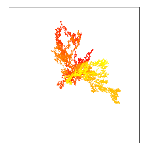
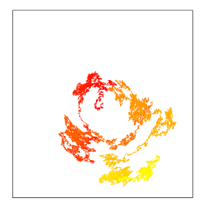
Figure 4: Simulation of the elliptic random walk in ${\mathbb{R}}^{2}$ for the recurrent case $a>b$ (left) and the transient case $a<b$ (right).

Remarks 3.3.

1. The process $X$ reduces to the classical PRRW when $a=b$: in that case it is spatially homogeneous, i.e., the distribution of the increment $X_{n+1}-X_{n}$ does not depend on $X_{n}$. For $a\neq b$ the random walk is not spatially homogeneous, and the jump distribution depends upon the projection onto the unit sphere of the walk’s current position.

2. As mentioned earlier, we choose to take increments as defined at (3.4), rather than increments that are uniform on the ellipse with respect to one-dimensional Lebesgue measure on $E_{\mathbf{x}}(a,b)$, purely for computational reasons. In fact, in two dimensions, since the Lebesgue measure on $E_{\mathbf{x}}(a,b)$ coincides with the measure induced by taking $\phi$ uniformly distributed on $(-\pi,\pi]$ when $a=b$, and the case $a=b$ is critically recurrent, the qualitative behaviour will be the same in either case: the walk will be transient for $a<b$ and recurrent for $a\geq b$. For higher dimensions, taking increments that are uniform with respect to the Lebesgue measure on $E_{\mathbf{x}}^{d}(a,b):=\{Q_{\hat{\mathbf{x}}}D{\mathbf{u}}:{\mathbf{u}}\in{\mathbb{S}}^{d-1}\}$ will still specify a family of models that exhibit a phase transition, from transience (for $a/b$ small) to recurrence (for $a/b$ large) but the exact shape of the ellipsoid in the critical case (i.e., the smallest ratio $a/b$ for which the walk is recurrent) may be different.

3. It follows from (3.2) that

   $$\|X_{n+1}\|^{2} =\|X_{n}\|^{2}+2\|X_{n}\|\langle\widehat{X}_{n},\Delta_{n}\rangle+\|\Delta_{n}\|^{2}$$

   $$=\|X_{n}\|^{2}+2\|X_{n}\|\langle{\mathbf{e}}_{1},D{\bm{\zeta}}_{n}\rangle+\langle{\bm{\zeta}}_{n},D^{2}{\bm{\zeta}}_{n}\rangle$$

   $$=\|X_{n}\|^{2}+2a\sqrt{d}\|X_{n}\|\langle{\mathbf{e}}_{1},{\bm{\zeta}}_{n}\rangle+(a^{2}-b^{2})d\langle{\mathbf{e}}_{1},{\bm{\zeta}}_{n}\rangle^{2}+b^{2}d.$$ (3.6)

   In particular, for this family of models $(\|X_{n}\|,n\in{\mathbb{Z}}_{+})$ is itself a Markov process, since the distribution of $\|X_{n+1}\|$ depends only on $\|X_{n}\|$ and not $X_{n}$; however, in the general setting of Section 2, this need not be the case.

   One-dimensional processes with evolutions reminiscent to that given by (3.6) have been studied previously by Kingman [11] and Bingham [2]. Those processes can be viewed, respectively, as the distance from its start point of a random walk in Euclidean space, and the geodesic distance from its start point of a random walk on the surface of a sphere, but in both cases the increments of the random walk have the property that the distribution of the jump vector is a product of the independent marginal distributions of the length and direction of the jump vector. In contrast, for the elliptic random walk the laws of $\|\Delta_{n}\|$ and $\langle\widehat{X}_{n},\widehat{\Delta}_{n}\rangle$ are not independent (except when $a=b$).

4. The theory equally applies to the case where the ellipsoid specifying the jump distribution is oriented with some fixed angle $\alpha\in[0,\pi)$ with respect to the radial direction. If we define $\Delta=Q^{\alpha}_{\hat{\mathbf{x}}}D{\bm{\zeta}}$, where $Q^{\alpha}_{\hat{\mathbf{x}}}$ is an orthogonal matrix that maps ${\mathbf{e}}_{\alpha}:={\mathbf{e}}_{1}\cos{\alpha}+{\mathbf{e}}_{2}\sin{\alpha}$ to $\hat{\mathbf{x}}$, then we find that transience of $X$ is equivalent to

   $$(a^{2}-b^{2})\cos{2\alpha}<(d-2)b^{2}.$$

   Note that for $d=2$, $Q^{\alpha}_{\hat{\mathbf{x}}}$ and therefore $\Delta$ are well defined, but this is not so for higher dimensions. Nevertheless, for any collection of matrices $(Q^{\alpha}_{{\mathbf{u}}};{\mathbf{u}}\in{\mathbb{S}}^{d-1})$ satisfying $Q^{\alpha}_{\mathbf{u}}{\mathbf{e}}_{\alpha}={\mathbf{u}}$ for all ${\mathbf{u}}\in{\mathbb{S}}^{d-1}$ we get the same recurrence classification. This is because the distribution of $\|X_{n+1}\|$ given $X_{n}$ is determined through the angle $\alpha$ via

   $$\|X_{n}\|^{2}+2\sqrt{d}\|X_{n}\|(a\langle{\mathbf{e}}_{1},{\bm{\zeta}}_{n}\rangle\cos{\alpha}+b\langle{\mathbf{e}}_{2},{\bm{\zeta}}_{n}\rangle\sin{\alpha})+(a^{2}-b^{2})d\langle{\mathbf{e}}_{1},{\bm{\zeta}}_{n}\rangle^{2}+b^{2}d,$$

   and therefore assumption ((A4)) holds with $U=a^{2}\cos^{2}{\alpha}+b^{2}\sin^{2}{\alpha}$ and $V=a^{2}+(d-1)b^{2}$.

4 Non-confinement

In this section we prove that the assumptions ((A0)), ((A1)), and ((A2)) imply that $\limsup_{n\to\infty}\|X_{n}\|=+\infty$, a.s. We first present a general result for martingales on ${\mathbb{R}}^{d}$ satisfying a “uniform dispersion” condition; the result can be viewed as a $d$-dimensional martingale version of Kolmogorov’s other inequality (see e.g. [5, pp. 123, 502]).

Lemma 4.1.

Let $d\in{\mathbb{N}}$. Suppose that $(Y_{n},n\in{\mathbb{Z}}_{+})$ is an ${\mathbb{R}}^{d}$-valued process adapted to a filtration $({\mathcal{G}}_{n},n\in{\mathbb{Z}}_{+})$, with ${\mathbb{P}}[Y_{0}={\mathbf{0}}\mid{\mathcal{G}}_{0}]=1$. Suppose that there exist $p>2,v>0,B<\infty$ such that for all $n\in{\mathbb{Z}}_{+}$, a.s.,

$$\operatorname{\mathbb{E}}[\|Y_{n+1}-Y_{n}\|^{p}\mid{\mathcal{G}}_{n}] \leq B;$$ (4.1)

$$\operatorname{\mathbb{E}}[\|Y_{n+1}-Y_{n}\|^{2}\mid{\mathcal{G}}_{n}] \geq v;$$ (4.2)

$$\operatorname{\mathbb{E}}[Y_{n+1}-Y_{n}\mid{\mathcal{G}}_{n}] ={\mathbf{0}}.$$ (4.3)

Then there exists $D<\infty$, depending only on $B$, $p$, and $v$, such that for all $n\in{\mathbb{Z}}_{+}$ and all $x\in{\mathbb{R}}_{+}$,

$${\mathbb{P}}\Bigl{[}\max_{0\leq\ell\leq n}\|Y_{\ell}\|\geq x\;\Bigl{|}\;{\mathcal{G}}_{0}\Bigr{]}\geq 1-\frac{D(1+x)^{2}}{n},\ \text{a.s.}$$

Proof.

Let $x>0$ and set $\tau=\min\{n\geq 0:\|Y_{n}\|\geq x\}$; throughout the paper we adopt the usual convention $\min\emptyset:=\infty$. In analogy with previous notation, write $\Delta_{n}=Y_{n+1}-Y_{n}$ for the jump distribution, and let

$$W_{n}=\begin{cases}Y_{n}&\text{if $\|Y_{n}\|\leq A(1+x)$},\\ Y_{n-1}+\widehat{\Delta}_{n-1}(A-1)(1+x)&\text{if $\|Y_{n}\|>A(1+x)$},\end{cases}$$

where $A>1$ is a constant to be specified later. Note that $W_{n}$ is ${\mathcal{G}}_{n}$-measurable.

Now, on $\{\|Y_{n}\|\leq x\}$, $W_{n}=Y_{n}$ and

$$\operatorname{\mathbb{E}}[W_{n+1}-W_{n}\mid{\mathcal{G}}_{n}]={} \operatorname{\mathbb{E}}[\Delta_{n}\mid{\mathcal{G}}_{n}]$$

$${}+\operatorname{\mathbb{E}}[\widehat{\Delta}_{n}\left((A-1)(1+x)-\|\Delta_{n}\|\right){\mathbf{1}}{\{\|Y_{n+1}\|>A(1+x)\}}\mid{\mathcal{G}}_{n}].$$

But $\{\|Y_{n+1}\|>A(1+x)\}\cap\{\|Y_{n}\|\leq x\}$ implies that $\|\Delta_{n}\|>(A-1)(1+x)$, and by (4.3), $\operatorname{\mathbb{E}}[\Delta_{n}\mid{\mathcal{G}}_{n}]={\mathbf{0}}$. Hence, on $\{\|Y_{n}\|\leq x\}$,

$$\bigl{\|}\operatorname{\mathbb{E}}[W_{n+1}-W_{n}\mid{\mathcal{G}}_{n}]\bigr{\|} \leq\operatorname{\mathbb{E}}[\|\Delta_{n}\|{\mathbf{1}}{\{\|\Delta_{n}\|>(A-1)(1+x)\}}\mid{\mathcal{G}}_{n}]$$

$$\leq(A-1)^{-1}(1+x)^{-1}\operatorname{\mathbb{E}}[\|\Delta_{n}\|^{2}\mid{\mathcal{G}}_{n}]$$

$$\leq B^{\prime}(A-1)^{-1}(1+x)^{-1},\ \text{a.s.},$$

where, by (4.1) and Lyapunov’s inequality, $B^{\prime}<\infty$ depends only on $B$ and $p$. Hence we can choose $A\geq A_{0}$ for some $A_{0}=A_{0}(B,p,v)$ large enough so that

$$\bigl{\|}\operatorname{\mathbb{E}}[W_{n+1}-W_{n}\mid{\mathcal{G}}_{n}]\bigr{\|}\leq(v/8)(1+x)^{-1},\text{ on }\{\|Y_{n}\|\leq x\}.$$ (4.4)

Also, on $\{\|Y_{n}\|\leq x\}$, by a similar argument,

$$\operatorname{\mathbb{E}}[\|W_{n+1}-W_{n}\|^{2}\mid{\mathcal{G}}_{n}]\bigr{\|} =\operatorname{\mathbb{E}}[\|\Delta_{n}\|^{2}\mid{\mathcal{G}}_{n}]$$

$$\quad+\operatorname{\mathbb{E}}[\left((A-1)^{2}(1+x)^{2}-\|\Delta_{n}\|^{2}\right){\mathbf{1}}{\{\|Y_{n+1}\|>A(1+x)\}}\mid{\mathcal{G}}_{n}]$$

$$\geq\operatorname{\mathbb{E}}[\|\Delta_{n}\|^{2}\mid{\mathcal{G}}_{n}]-\operatorname{\mathbb{E}}[\|\Delta_{n}\|^{2}{\mathbf{1}}{\{\|\Delta_{n}\|>(A-1)(1+x)\}}\mid{\mathcal{G}}_{n}]$$

$$\geq v-(A-1)^{2-p}(1+x)^{2-p}\operatorname{\mathbb{E}}[\|\Delta_{n}\|^{p}\mid{\mathcal{G}}_{n}]$$

$$\geq v/2,$$ (4.5)

for all $x\geq 0$ and $A\geq A_{1}$ for sufficiently large $A_{1}=A_{1}(B,p,v)$, using (4.1) and (4.2).

Now, set $Z_{n}=\|W_{n\wedge\tau}\|^{2}$. Then, on $\{n<\tau\}$, by (4.4) and (4.4),

$$\operatorname{\mathbb{E}}[Z_{n+1}-Z_{n}\mid{\mathcal{G}}_{n}] =\operatorname{\mathbb{E}}[\|W_{n+1}\|^{2}-\|W_{n}\|^{2}\mid{\mathcal{G}}_{n}]$$

$$=\operatorname{\mathbb{E}}[\|W_{n+1}-W_{n}\|^{2}\mid{\mathcal{G}}_{n}]+2\bigl{\langle}W_{n},\operatorname{\mathbb{E}}[W_{n+1}-W_{n}\mid{\mathcal{G}}_{n}]\bigr{\rangle}$$

$$\geq\frac{v}{2}-\frac{2\|W_{n}\|v}{8(1+x)}\geq\frac{v}{2}-\frac{vx}{4(1+x)}\geq\frac{v}{4}.$$

Hence $Z_{n}-\sum_{k=0}^{n-1}v_{k}$ is a ${\mathcal{G}}_{n}$-adapted submartingale, where

$$v_{k}=\frac{v}{4}{\mathbf{1}}{\{k<\tau\}}\geq\frac{v}{4}{\mathbf{1}}{\{n<\tau\}},\leavevmode\nobreak\ \leavevmode\nobreak\ \text{for}\leavevmode\nobreak\ 0\leq k<n.$$

By construction, $0\leq Z_{n}\leq A^{2}(1+x)^{2}$, so

$$0=\operatorname{\mathbb{E}}[Z_{0}\mid{\mathcal{G}}_{0}]\leq\operatorname{\mathbb{E}}[Z_{n}\mid{\mathcal{G}}_{0}]-\sum_{k=0}^{n-1}\operatorname{\mathbb{E}}[v_{k}\mid{\mathcal{G}}_{0}]\leq A^{2}(1+x)^{2}-\sum_{k=0}^{n-1}\frac{v}{4}{\mathbb{P}}[n<\tau\mid{\mathcal{G}}_{0}],$$

which implies $n(v/4){\mathbb{P}}[n<\tau\mid{\mathcal{G}}_{0}]\leq A^{2}(1+x)^{2}$. In other words,

$${\mathbb{P}}\Bigl{[}\max_{0\leq\ell\leq n}\|Y_{\ell}\|<x\;\Bigl{|}\;{\mathcal{G}}_{0}\Bigr{]}\leq\frac{4A^{2}(1+x)^{2}}{vn},\ \text{a.s.}\qed$$

Now we can give the proof of Proposition 2.1.

Proof of Proposition 2.1..

It is enough to show that for all $x\in{\mathbb{R}}_{+}$ the event $\{\|X_{n}\|\geq x\}$ occurs infinitely often. For a given $x$, we will apply Lemma 4.1 to $Y_{n}=X_{m+n}-X_{m}$ with ${\mathcal{G}}_{n}=\sigma(X_{0},\dots,X_{m+n})$; that result is applicable, since ((A0)), ((A1)) and ((A2)) imply (4.1), (4.3) and (4.2), respectively. Thus Lemma 4.1 shows that, for some finite $t=t(x)$,

$${\mathbb{P}}{\Bigl{[}\max_{0\leq\ell\leq t-1}\|X_{m+\ell}-X_{m}\|\geq 2x\;\Bigl{|}\;X_{0},\dots,X_{m}\Bigr{]}}\geq\frac{1}{2},\ \text{a.s.},$$ (4.6)

for all $m\geq 0$. For $k=1,2,\dotsc$, define the event

$$A_{k}=\Bigl{\{}\max_{0\leq\ell\leq t-1}\|X_{(k-1)t+\ell}-X_{(k-1)t}\|\geq 2x\Bigr{\}},$$

and filtration ${\mathcal{G}}^{\prime}_{k-1}=\sigma(X_{0},\dots,X_{(k-1)t})$. Then $A_{k}\in{\mathcal{G}}^{\prime}_{k}$, and, by (4.6), ${\mathbb{P}}{[A_{k}\mid{\mathcal{G}}^{\prime}_{k-1}]}\geq\frac{1}{2}$, a.s., for all $k$. An application of Lévy’s extension of the Borel–Cantelli lemma (see, e.g., [9, Cor. 7.20]) shows that $A_{k}$ occurs infinitely often, a.s. For each $k$ such that $A_{k}$ occurs, either

• $\|X_{(k-1)t}\|\geq x$, or

• $\|X_{(k-1)t}\|\leq x$ and $\|X_{n}\|\geq x$ for some $(k-1)t<n<kt$.

Since one of these cases must occur for infinitely many $k$, we have that $\{\|X_{n}\|\geq x\}$ occurs infinitely often, as required. ∎

5 Recurrence classification

In this section we study the random walk $X_{n}$ and give the proof of the recurrence classification, Theorem 2.3. The method of proof is based on applying classical results of Lamperti [12] to the ${\mathbb{R}}_{+}$-valued radial process given by $R_{n}:=\|X_{n}\|$. The method rests on an analysis of the increments $R_{n+1}-R_{n}$ given $X_{n}={\mathbf{x}}\in{\mathbb{X}}$; in general, $R_{n}$ is not itself a Markov process. The following notation will be useful. Given ${\mathbf{x}}\neq{\mathbf{0}}$ and ${\mathbf{y}}\in{\mathbb{R}}^{d}$, write

$${\mathbf{y}}_{\mathbf{x}}:=\frac{\langle{\mathbf{x}},{\mathbf{y}}\rangle}{\|{\mathbf{x}}\|}=\langle\hat{\mathbf{x}},{\mathbf{y}}\rangle,$$

so that ${\mathbf{y}}_{\mathbf{x}}$ is the component of ${\mathbf{y}}$ in the $\hat{\mathbf{x}}$ direction, and ${\mathbf{y}}-{\mathbf{y}}_{\mathbf{x}}\,\hat{\mathbf{x}}$ is a vector perpendicular to $\hat{\mathbf{x}}$.

First we state a general result on the increments of $R_{n}$ for a Markov process $X_{n}$ on ${\mathbb{X}}$. Recall that we write $\Delta=X_{1}-X_{0}$, and let $\Delta_{\mathbf{x}}$ be the radial component of $\Delta$ at $X_{0}={\mathbf{x}}$ in accordance with the notation described above; no confusion should arise with our notation $\Delta_{n}$ defined previously.

We make an important comment on notation. When we write $O(\|{\mathbf{x}}\|^{-1-\delta})$, and similar expressions, these are understood to be uniform in ${\mathbf{x}}$. That is, if $f:{\mathbb{R}}^{d}\to{\mathbb{R}}$ and $g:{\mathbb{R}}_{+}\to{\mathbb{R}}_{+}$, we write $f({\mathbf{x}})=O(g(\|{\mathbf{x}}\|))$ to mean that there exist $C\in{\mathbb{R}}_{+}$ and $r\in{\mathbb{R}}_{+}$ such that

$$|f({\mathbf{x}})|\leq Cg(\|{\mathbf{x}}\|)\text{ for all }{\mathbf{x}}\in{\mathbb{X}}\text{ with }\|{\mathbf{x}}\|\geq r.$$ (5.1)

Lemma 5.1.

Suppose that $X$ is a discrete-time, time-homogeneous Markov process on ${\mathbb{X}}\subseteq{\mathbb{R}}^{d}$ satisfying ((A0)) for some $p>2$. Then, for $R_{n}:=\|X_{n}\|$, we have

$$\sup_{{\mathbf{x}}\in{\mathbb{X}}}\operatorname{\mathbb{E}}[|R_{n+1}-R_{n}|^{p}\mid X_{n}={\mathbf{x}}]<\infty,$$ (5.2)

and the radial increment moment functions satisfy

$$\mu_{1}({\mathbf{x}}) :=\operatorname{\mathbb{E}}[R_{n+1}-R_{n}\mid X_{n}={\mathbf{x}}]=\operatorname{\mathbb{E}}_{\mathbf{x}}[\Delta_{\mathbf{x}}]+\frac{\operatorname{\mathbb{E}}_{\mathbf{x}}[\|\Delta\|^{2}-\Delta^{2}_{{\mathbf{x}}}]}{2\|{\mathbf{x}}\|}+O(\|{\mathbf{x}}\|^{-1-\delta}),$$ (5.3)

$$\mu_{2}({\mathbf{x}}) :=\operatorname{\mathbb{E}}[(R_{n+1}-R_{n})^{2}\mid X_{n}={\mathbf{x}}]=\operatorname{\mathbb{E}}_{\mathbf{x}}[\Delta_{\mathbf{x}}^{2}]+O(\|{\mathbf{x}}\|^{-\delta}),$$ (5.4)

as $\|{\mathbf{x}}\|\to\infty$, for some $\delta=\delta(p)>0$.

Proof.

By time-homogeneity, it suffices to consider the case $n=0$. By the triangle inequality, $|R_{1}-R_{0}|=\bigl{|}\|X_{0}+\Delta\|-\|X_{0}\|\bigr{|}\leq\|\Delta\|$, so that (5.2) follows from ((A0)).

We prove (5.3) and (5.4) by approximating

$$\begin{split}\|{\mathbf{x}}+\Delta\|-\|{\mathbf{x}}\|&=\sqrt{\langle{\mathbf{x}}+\Delta,{\mathbf{x}}+\Delta\rangle}-\|{\mathbf{x}}\|\\ &=\|{\mathbf{x}}\|\left[\left(1+\frac{2\Delta_{\mathbf{x}}}{\|{\mathbf{x}}\|}+\frac{\|\Delta\|^{2}}{\|{\mathbf{x}}\|^{2}}\right)^{1/2}-1\right]\end{split}$$ (5.5)

for large ${\mathbf{x}}$. Let $A_{\mathbf{x}}=\{\|\Delta\|\leq\|{\mathbf{x}}\|^{\beta}\}$ for some $\beta\in(0,1)$ to be determined later. On the event $A_{\mathbf{x}}$ we approximate (5.5) using Taylor’s formula for $(1+y)^{1/2}$, and on the event $A_{\mathbf{x}}^{{\mathrm{c}}}$ we bound (5.5) using ((A0)).

Indeed, for all $y>-1$, Taylor’s theorem with Lagrange remainder shows that

$$(1+y)^{1/2}=1+\frac{1}{2}y-\frac{1}{8}y^{2}(1+\gamma y)^{-3/2},$$

for some $\gamma=\gamma(y)\in[0,1]$, so on the event $A_{\mathbf{x}}$,

$$\|{\mathbf{x}}+\Delta\|-\|{\mathbf{x}}\| =\|{\mathbf{x}}\|\left(\frac{\Delta_{\mathbf{x}}}{\|{\mathbf{x}}\|}+\frac{\|\Delta\|^{2}}{2\|{\mathbf{x}}\|^{2}}-\frac{1}{8}\left(\frac{2\Delta_{\mathbf{x}}}{\|{\mathbf{x}}\|}+\frac{\|\Delta\|^{2}}{\|{\mathbf{x}}\|^{2}}\right)^{2}\left(1+O(\|{\mathbf{x}}\|^{\beta-1})\right)\right)$$

$$=\Delta_{\mathbf{x}}+\frac{\|\Delta\|^{2}}{2\|{\mathbf{x}}\|}-\frac{\|{\mathbf{x}}\|}{8}\left(\frac{4\Delta_{\mathbf{x}}^{2}}{\|{\mathbf{x}}\|^{2}}+\frac{\|\Delta\|^{2}}{\|{\mathbf{x}}\|^{2}}\left(\frac{4\Delta_{\mathbf{x}}}{\|{\mathbf{x}}\|}+\frac{\|\Delta\|^{2}}{\|{\mathbf{x}}\|^{2}}\right)\right)\left(1+O(\|{\mathbf{x}}\|^{\beta-1})\right)$$

$$=\Delta_{\mathbf{x}}+\frac{\|\Delta\|^{2}}{2\|{\mathbf{x}}\|}-\frac{\Delta_{\mathbf{x}}^{2}}{2\|{\mathbf{x}}\|}\left(1+O(\|{\mathbf{x}}\|^{\beta-1})\right)+\frac{\|\Delta\|^{2}}{\|{\mathbf{x}}\|}O(\|{\mathbf{x}}\|^{\beta-1})$$

$$=\Delta_{\mathbf{x}}+\left(\frac{\|\Delta\|^{2}-\Delta_{\mathbf{x}}^{2}}{2\|{\mathbf{x}}\|}\right)\left(1+O(\|{\mathbf{x}}\|^{\beta-1})\right),$$ (5.6)

where the error terms follow from the fact that $|\Delta_{\mathbf{x}}|\leq\|\Delta\|\leq\|{\mathbf{x}}\|^{\beta}$ for $\beta<1$.

On the other hand,

$$\bigl{|}\|{\mathbf{x}}+\Delta\|-\|{\mathbf{x}}\|\bigr{|}{\mathbf{1}}{(A_{\mathbf{x}}^{{\mathrm{c}}})}\leq\|\Delta\|{\mathbf{1}}{(A_{\mathbf{x}}^{{\mathrm{c}}})}=\|\Delta\|^{p}\|\Delta\|^{1-p}{\mathbf{1}}{(A_{\mathbf{x}}^{{\mathrm{c}}})}\leq\|\Delta\|^{p}\|{\mathbf{x}}\|^{\beta(1-p)},$$ (5.7)

by the triangle inequality and the fact that $\|\Delta\|>\|{\mathbf{x}}\|^{\beta}$ on $A_{\mathbf{x}}^{{\mathrm{c}}}$. Since

$$\|{\mathbf{x}}+\Delta\|-\|{\mathbf{x}}\|=(\|{\mathbf{x}}+\Delta\|-\|{\mathbf{x}}\|){\mathbf{1}}{(A_{\mathbf{x}})}+(\|{\mathbf{x}}+\Delta\|-\|{\mathbf{x}}\|){\mathbf{1}}{(A_{\mathbf{x}}^{{\mathrm{c}}})},$$

we can combine (5) and (5.7) to give

$$\biggl{|}\|{\mathbf{x}}+\Delta\|\biggr{.} -\biggl{.}\|{\mathbf{x}}\|-\left[\Delta_{\mathbf{x}}+\left(\frac{\|\Delta\|^{2}-\Delta_{\mathbf{x}}^{2}}{2\|{\mathbf{x}}\|}\right)\left(1+O(\|{\mathbf{x}}\|^{\beta-1})\right)\right]\biggr{|}$$

$$=\biggl{|}\|{\mathbf{x}}+\Delta\|-\|{\mathbf{x}}\|-\left[\Delta_{\mathbf{x}}+\left(\frac{\|\Delta\|^{2}-\Delta_{\mathbf{x}}^{2}}{2\|{\mathbf{x}}\|}\right)\left(1+O(\|{\mathbf{x}}\|^{\beta-1})\right)\right]\biggr{|}{\mathbf{1}}{(A_{\mathbf{x}}^{{\mathrm{c}}})}$$

$$\leq\|\Delta\|^{p}\|{\mathbf{x}}\|^{\beta(1-p)}+\left|\Delta_{\mathbf{x}}+\left(\frac{\|\Delta\|^{2}-\Delta_{\mathbf{x}}^{2}}{2\|{\mathbf{x}}\|}\right)\left(1+O(\|{\mathbf{x}}\|^{\beta-1})\right)\right|{\mathbf{1}}{(A_{\mathbf{x}}^{{\mathrm{c}}})}$$

$$\leq 2\|\Delta\|^{p}\|{\mathbf{x}}\|^{\beta(1-p)}+\frac{\|\Delta\|^{p}}{2\|{\mathbf{x}}\|}\left(1+O(\|{\mathbf{x}}\|^{\beta-1})\right)\|{\mathbf{x}}\|^{\beta(2-p)}.$$

Therefore, taking expectations and using ((A0)), we obtain

$$\mu_{1}({\mathbf{x}})=\operatorname{\mathbb{E}}_{\mathbf{x}}[\Delta_{\mathbf{x}}]+\frac{\operatorname{\mathbb{E}}_{\mathbf{x}}[\|\Delta\|^{2}-\Delta_{\mathbf{x}}^{2}]}{2\|{\mathbf{x}}\|}+O(\|{\mathbf{x}}\|^{\beta-2})+O(\|{\mathbf{x}}\|^{\beta(1-p)})+O(\|{\mathbf{x}}\|^{\beta(2-p)-1}).$$

Taking $\beta=2/p$ makes all the error terms of size $O(\|{\mathbf{x}}\|^{-1-\delta})$ for some $\delta=\delta(p)>0$, namely for $\delta=(p-2)/p$.

For the second moment, we use the identity

$$\begin{split}(\|{\mathbf{x}}+\Delta\|-\|{\mathbf{x}}\|)^{2}&=\|{\mathbf{x}}+\Delta\|^{2}-\|{\mathbf{x}}\|^{2}-2\|{\mathbf{x}}\|(\|{\mathbf{x}}+\Delta\|-\|{\mathbf{x}}\|)\\ &=2\|{\mathbf{x}}\|\Delta_{\mathbf{x}}+\|\Delta\|^{2}-2\|{\mathbf{x}}\|(\|{\mathbf{x}}+\Delta\|-\|{\mathbf{x}}\|),\end{split}$$

so that

$$\mu_{2}({\mathbf{x}})=2\|{\mathbf{x}}\|\operatorname{\mathbb{E}}_{\mathbf{x}}[\Delta_{\mathbf{x}}]+\operatorname{\mathbb{E}}_{\mathbf{x}}[\|\Delta\|^{2}]-2\|{\mathbf{x}}\|\mu_{1}({\mathbf{x}})=\operatorname{\mathbb{E}}_{\mathbf{x}}[\Delta_{\mathbf{x}}^{2}]+O(\|{\mathbf{x}}\|^{-\delta}),$$

as required. ∎

With the additional assumptions ((A1)), ((A3)), and ((A4)), we can use Lemma 5.1 to prove the following result.

Lemma 5.2.

Suppose that $X$ is a discrete-time, time-homogeneous Markov process on ${\mathbb{X}}\subseteq{\mathbb{R}}^{d}$ satisfying ((A0)), ((A1)), ((A3)), and ((A4)). Then, with $\mu_{1},\mu_{2}$ defined at (5.3), (5.4), and $\varepsilon(r)$ defined at ((A3)), there exists $\delta>0$ such that, as $\|{\mathbf{x}}\|\to\infty$,

$$2\|{\mathbf{x}}\|\mu_{1}({\mathbf{x}})=V-U+O(\varepsilon(\|{\mathbf{x}}\|))+O(\|{\mathbf{x}}\|^{-\delta}),\leavevmode\nobreak\ \leavevmode\nobreak\ \mu_{2}({\mathbf{x}})=U+O(\varepsilon(\|{\mathbf{x}}\|))+O(\|{\mathbf{x}}\|^{-\delta}).$$ (5.8)

Proof.

By definition of $\varepsilon(r)$ at ((A3)) we have $\|M({\mathbf{x}})-\sigma^{2}(\hat{\mathbf{x}})\|_{\rm op}=O(\varepsilon(\|{\mathbf{x}}\|))$ as $\|{\mathbf{x}}\|\to\infty$. Then ((A4)) implies that

$$\begin{split}\operatorname{\mathbb{E}}_{{\mathbf{x}}}[\|\Delta\|^{2}]&=\operatorname{tr}{(M({\mathbf{x}}))}\\ &=\operatorname{tr}{(\sigma^{2}(\hat{\mathbf{x}}))}+O(\varepsilon(\|{\mathbf{x}}\|))\\ &=V+O(\varepsilon(\|{\mathbf{x}}\|)),\end{split}$$

and

$$\begin{split}\operatorname{\mathbb{E}}_{{\mathbf{x}}}[\Delta_{\mathbf{x}}^{2}]&=\langle\hat{\mathbf{x}},M({\mathbf{x}})\cdot\hat{\mathbf{x}}\rangle\\ &=\langle\hat{\mathbf{x}},\sigma^{2}(\hat{\mathbf{x}})\cdot\hat{\mathbf{x}}\rangle+O(\varepsilon(\|{\mathbf{x}}\|))\\ &=U+O(\varepsilon(\|{\mathbf{x}}\|)),\end{split}$$

and ((A1)) implies that $\operatorname{\mathbb{E}}_{{\mathbf{x}}}[\Delta_{\mathbf{x}}]=\operatorname{\mathbb{E}}_{{\mathbf{x}}}[\langle\Delta,\hat{\mathbf{x}}\rangle]=\langle\mu({\mathbf{x}}),\hat{\mathbf{x}}\rangle=0$. Using these expressions in Lemma 5.1 yields (5.8). ∎

Now we can complete the proof of Theorem 2.3.

Proof of Theorem 2.3..

We apply Lamperti’s [12] recurrence classification to $R_{n}=\|X_{n}\|$, the radial process. Proposition 2.1 shows that $\limsup_{n\to\infty}R_{n}=+\infty$, and Lemma 5.1 tells us that (5.2) is satisfied.

Because the error terms in (5.8) are uniform in ${\mathbf{x}}$, Lemma 5.2 shows that for all $\eta>0$ there exists $C<\infty$ such that

$$2\|{\mathbf{x}}\|\mu_{1}({\mathbf{x}})-\mu_{2}({\mathbf{x}})\in[V-2U-\eta,V-2U+\eta]$$

for all ${\mathbf{x}}\in{\mathbb{X}}$ with $\|{\mathbf{x}}\|\geq C$. Therefore, it follows from Theorem 3.2 of [12] that $X$ is transient if $V-2U>0$ and recurrent if $V-2U<0$. For the boundary case, when $V-2U=0$, if $\varepsilon(r)=O(r^{-\delta_{0}})$ then

$$2\|{\mathbf{x}}\|\mu_{1}({\mathbf{x}})-\mu_{2}({\mathbf{x}})=O(\|{\mathbf{x}}\|^{-\delta_{1}}),$$

for $\delta_{1}=\min\{\delta,\delta_{0}\}$, which implies that $X$ is recurrent, again by Theorem 3.2 of [12]. ∎

6 Nullity

In this section we give the proof of Theorem 2.4. In the transient case, this is straightforward.

Lemma 6.1.

In case (i) of Theorem 2.3, for any bounded $A\subset{\mathbb{R}}^{d}$, as $n\to\infty$, the null property (2.2) holds.

Proof.

It is sufficient to prove (2.2) in the case where $A=B_{r}:=\{{\mathbf{x}}\in{\mathbb{X}}:\|{\mathbf{x}}\|\leq r\}$. In case (i), $X$ is transient, meaning that $\|X_{n}\|\to\infty$ a.s., so that ${\mathbf{1}}{\{X_{n}\in B_{r}\}}\to 0$, a.s., for any $r\in{\mathbb{R}}_{+}$. Hence the Cesàro limit in (2.2) is also $0$, a.s., and the $L^{q}$ convergence follows from the bounded convergence theorem. ∎

It remains to consider cases (ii) and (iii), when $X$ is recurrent. Thus there exists $r_{0}\in{\mathbb{R}}_{+}$ such that $\liminf_{n\to\infty}\|X_{n}\|\leq r_{0}$, a.s. Let $\tau_{r}:=\min\{n\in{\mathbb{Z}}_{+}:X_{n}\in B_{r}\}$. It suffices to take $A=B_{r}$, $r>r_{0}$, so $X_{n}\in B_{r}$ infinitely often. We make the following claim, whose proof is deferred until the end of this section, which says that if the walk has not yet entered a ball of radius $R$ (for any $R>r$ big enough), the time until it reaches the ball of radius $r$ has tail bounded below as displayed.

Lemma 6.2.

In cases (ii) and (iii) of Theorem 2.3, there exists a finite $r_{1}\geq r_{0}$ such that for any $r>r_{1}$ and $R>r$ there exists a finite positive $c$ such that

$${\mathbb{P}}[\tau_{r}\geq n+m\mid X_{0},\ldots,X_{n}]\geq cm^{-1/2},\text{ on }\{n<\tau_{R}\},$$ (6.1)

for all sufficiently large $m$.

Assuming this result, we can complete the proof of Theorem 2.4.

Proof of Theorem 2.4..

In case (i), the result is contained in Lemma 6.1. So consider cases (ii) and (iii). Fix $r$ and $R$ with $R>r>r_{1}$, with $r_{1}$ as in Lemma 6.2. Note that $\liminf_{n\to\infty}\|X_{n}\|\leq r_{0}\leq r_{1}$, a.s.

Set $\gamma_{1}:=0$ and then define recursively, for $\ell\in{\mathbb{N}}$, the stopping times

$$\eta_{\ell}:=\min\{n\geq\gamma_{\ell}:X_{n}\notin B_{R}\},\leavevmode\nobreak\ \leavevmode\nobreak\ \leavevmode\nobreak\ \gamma_{\ell+1}:=\min\{n\geq\eta_{\ell}:X_{n}\in B_{r}\},$$

with the convention that $\min\emptyset:=\infty$. Since $r>r_{0}$ and $\limsup_{n\to\infty}\|X_{n}\|=\infty$ (by Proposition 2.1), for all $\ell\in{\mathbb{N}}$ we have $\eta_{\ell}<\infty$ and $\gamma_{\ell}<\infty$, a.s., and

$$0=\gamma_{1}<\eta_{1}<\gamma_{2}<\eta_{2}<\cdots.$$

In particular, $\lim_{\ell\to\infty}\gamma_{\ell}=\lim_{\ell\to\infty}\eta_{\ell}=\infty$, a.s.

We now write ${\mathcal{F}}_{n}:=\sigma(X_{0},\ldots,X_{n})$. We use Lemma 4.1 to show that the process must exit from $B_{R}$ rapidly enough. Indeed, if $\kappa$ is any finite stopping time, set $Y_{n}=X_{\kappa+n}-X_{\kappa}$ and ${\mathcal{G}}_{n}={\mathcal{F}}_{\kappa+n}$. Then the assumptions ((A0)), ((A1)) and ((A2)) show that the hypotheses of Lemma 4.1 are satisfied, since, for example,

$$\operatorname{\mathbb{E}}[\|Y_{n+1}-Y_{n}\|^{p}\mid{\mathcal{G}}_{n}]=\operatorname{\mathbb{E}}[\|X_{\kappa+n+1}-X_{\kappa+n}\|^{p}\mid{\mathcal{F}}_{\kappa+n}]=\operatorname{\mathbb{E}}_{X_{\kappa+n}}[\|\Delta\|^{p}],$$

by the strong Markov property for $X$ at the finite stopping time ${\kappa+n}$. In particular, another application of Lemma 4.1, similarly to (4.6), shows that we may choose $n=n(R)\in{\mathbb{N}}$ sufficiently large so that

$${\mathbb{P}}\Bigl{[}\max_{0\leq\ell\leq n(R)}\|X_{\kappa+\ell}-X_{\kappa}\|\geq 2R\;\Bigl{|}\;{\mathcal{F}}_{\kappa}\Bigr{]}\geq\frac{1}{2},\ \text{a.s.},$$ (6.2)

an event whose occurrence ensures that if $X_{\kappa}\in B_{R}$, then $X$ exits $B_{R}$ before time $\kappa+n(R)$. Fix $k\in{\mathbb{N}}$. Then, an application of (6.2) at stopping time $\kappa=\gamma_{k}$ shows that

$${\mathbb{P}}[\eta_{k}-\gamma_{k}>n(R)\mid{\mathcal{F}}_{\gamma_{k}}]\leq{\mathbb{P}}\Bigl{[}\max_{0\leq\ell\leq n(R)}\|X_{{\gamma_{k}}+\ell}-X_{\gamma_{k}}\|<2R\;\Bigl{|}\;{\mathcal{F}}_{\gamma_{k}}\Bigr{]}\leq\frac{1}{2},\ \text{a.s.}$$

Similarly,

$${\mathbb{P}}[\eta_{k}-\gamma_{k}>2n(R)\mid{\mathcal{F}}_{\gamma_{k}}] =\operatorname{\mathbb{E}}\bigl{[}{\mathbf{1}}{\{\eta_{k}-\gamma_{k}>n(R)\}}\operatorname{\mathbb{E}}[{\mathbf{1}}{\{\eta_{k}-\gamma_{k}>2n(R)\}}\mid{\mathcal{F}}_{\gamma_{k}+n(R)}]\;\bigl{|}\;{\mathcal{F}}_{\gamma_{k}}\bigr{]}$$

$$\leq\frac{1}{2}{\mathbb{P}}[\eta_{k}-\gamma_{k}>n(R)\mid{\mathcal{F}}_{\gamma_{k}}]\leq\frac{1}{4},$$

this time applying (6.2) at stopping time $\kappa=\gamma_{k}+n(R)$ as well. Iterating this argument, it follows that ${\mathbb{P}}[\eta_{k}-\gamma_{k}>m\cdot n(R)\mid{\mathcal{F}}_{\gamma_{k}}]\leq 2^{-m}$, a.s., for all $m\in{\mathbb{N}}$. From here, it is straightforward to deduce that, for some constant $C<\infty$, for any $k\in{\mathbb{N}}$,

$$\operatorname{\mathbb{E}}[\eta_{k}-\gamma_{k}\mid{\mathcal{F}}_{\gamma_{k}}]\leq C,\ \text{a.s.}$$ (6.3)

On the other hand, the tail estimate (6.1) implies that

$${\mathbb{P}}[\gamma_{k+1}-\eta_{k}\geq m\mid{\mathcal{F}}_{\eta_{k}}]\geq cm^{-1/2},\ \text{a.s.},$$ (6.4)

for $c>0$ and all sufficiently large $m$.

For any $n\in{\mathbb{N}}$, set $k(n):=\min\{k\geq 2:\gamma_{k}>n\}$, so that $\gamma_{k(n)-1}\leq n<\gamma_{k(n)}$ for $k(n)\in\{2,3,\ldots\}$. Note $k(n)<\infty$ and $\lim_{n\to\infty}k(n)=\infty$, a.s. Then we claim

$$\frac{1}{n}\sum_{k=0}^{n-1}{\mathbf{1}}{\{X_{k}\in B_{r}\}}\leq\frac{\sum_{k=1}^{k(n)-1}\left(\eta_{k}-\gamma_{k}\right)}{\sum_{k=1}^{k(n)-2}\left(\gamma_{k+1}-\eta_{k}\right)}.$$ (6.5)

This is easiest to see by considering two separate cases. First, if $\eta_{k(n)-1}<n<\gamma_{k(n)}$,

$$\frac{1}{n}\sum_{k=0}^{n-1}{\mathbf{1}}{\{X_{k}\in B_{r}\}}\leq\frac{1}{\eta_{k(n)-1}}\sum_{k=0}^{\eta_{k(n)-1}}{\mathbf{1}}{\{X_{k}\in B_{r}\}},$$

which implies (6.5), since the set of $k$ less than $n$ for which $X_{k}\in B_{r}$ is contained in the set $\cup_{k=1}^{k(n)-1}[\gamma_{k},\eta_{k})$. On the other hand, if $\gamma_{k(n)-1}\leq n\leq\eta_{k(n)-1}$, using the elementary inequality $\frac{a}{b}\leq\frac{a+c}{b+c}$ for non-negative $a,b,c$ with $a/b\leq 1$, we have

$$\frac{1}{n}\sum_{k=0}^{n-1}{\mathbf{1}}{\{X_{k}\in B_{r}\}}\leq\frac{1}{\eta_{k(n)-1}}\left(\sum_{k=0}^{n-1}{\mathbf{1}}{\{X_{k}\in B_{r}\}}+(\eta_{k(n)-1}-n)\right),$$

which again gives (6.5).

To estimate the growth rates of the numerator and denominator of the right-hand side of (6.5), we apply some results from [6]. First, writing $Z_{m}=\sum_{k=1}^{m-1}(\eta_{k}-\gamma_{k})$ and ${\mathcal{G}}_{m}={\mathcal{F}}_{\gamma_{m}}$, by (6.3) we can apply Theorem 2.4 of [6] to the ${\mathcal{G}}_{m}$-adapted process $Z_{m}$ to obtain that for any $\varepsilon>0$, a.s., for all but finitely many $m$,

$$\sum_{k=1}^{m-1}\left(\eta_{k}-\gamma_{k}\right)\leq m^{1+\varepsilon}.$$

On the other hand, writing $Z_{m}=\sum_{k=1}^{m-1}(\gamma_{k+1}-\eta_{k})$ and ${\mathcal{G}}_{m}={\mathcal{F}}_{\eta_{m}}$, by (6.4) we can apply Theorem 2.6 of [6] to the ${\mathcal{G}}_{m}$-adapted process $Z_{m}$ to obtain that for any $\varepsilon>0$, for all $m$ sufficiently large,

$$\sum_{k=1}^{m-1}\left(\gamma_{k+1}-\eta_{k}\right)\geq m^{2-\varepsilon}.$$

Now (6.5) gives the almost-sure version of the result (2.2). The $L^{q}$ version follows from the bounded convergence theorem. ∎

It remains to complete the proof of Lemma 6.2. A more general, two-sided version of the inequality in Lemma 6.2 is proved in [7, Theorem 2.4] but under slightly different assumptions. Because of this, we cannot apply that result directly; nevertheless, the proof techniques naturally transfer to our setting. In doing so, the arguments become simpler to apply, so we reproduce them here.

Proof of Lemma 6.2.

By the Markov property for $X$ it is enough to prove the statement for $n=0$, namely that there exists finite $r_{1}\geq r_{0}$ such that for any $r>r_{1}$ and $R>r$ there exists a finite positive constant $c$ such that, if $X_{0}\not\in B_{R}$ then

$${\mathbb{P}}[\tau_{r}>m\mid X_{0}]\geq cm^{-1/2},$$

for sufficiently large $m$.

We outline the two intuitive steps in the proof. First we show that the probability that $\max_{0\leq k\leq\tau_{r}}\|X_{k}\|$ exceeds some large $x$ is bounded below by a constant times $1/x$. Second, we show that if the latter event does occur, with probability at least $1/2$ it takes the process time at least a constant times $x^{2}$ to reach $B_{r}$. Combining these two estimates will show that with probability of order $1/x$ the walk takes time of order $x^{2}$ to reach $B_{r}$, which gives the desired tail bound. Roughly speaking, the first estimate (reaching distance $x$) is provided by the optional stopping theorem and the fact that $\|X_{k}\|$ is a submartingale (cf. [7, Theorem 2.3]), and the second (taking quadratic time to return) is provided by a maximal inequality applied to an appropriate quadratic displacement functional (cf. [7, Lemma 4.11]). A technicality required for the first estimate is that to apply optional stopping, we need uniform integrability; so we actually work with a truncated version of $\|X_{k}\|$.

We now give the details. Recall that $R_{k}=\|X_{k}\|$ and let ${\mathcal{F}}_{k}=\sigma(X_{0},\dots,X_{k})$. Lemmas 5.1 and 5.2, with the fact that $V>U$ by ((A4)), imply that

$$\operatorname{\mathbb{E}}[R_{k+1}-R_{k}\mid{\mathcal{F}}_{k}]\geq\frac{2\varepsilon}{R_{k}}+o(R_{k}^{-1})\geq\frac{\varepsilon}{R_{k}},$$ (6.6)

for all $R_{k}>r_{1}$, for sufficiently large $r_{1}\geq r_{0}$ and some positive constant $\varepsilon$. Now, suppose that $r$ and $R$ satisfy $R>r>r_{1}$ and fix $x$ with $x\gg R$. Set $R_{k}^{x}:=\min\{2x,R_{k}\}$ and $\sigma_{x}:=\min\{k\geq 0:R_{k}>x\}$. Since $X_{k}$ is a martingale, we have that $R_{k}$ is a submartingale, as is the stopped process $Y_{k}:=R_{k\wedge\tau_{r}\wedge\sigma_{x}}$. In order to achieve uniform integrability, we consider the truncated process $Y_{k}^{x}:=R_{k\wedge\tau_{r}\wedge\sigma_{x}}^{x}$ and show that this is a submartingale.

For $k\geq\tau_{r}\wedge\sigma_{x}$, we have $Y_{k+1}^{x}-Y_{k}^{x}=0$ so $\operatorname{\mathbb{E}}[Y_{k+1}^{x}-Y_{k}^{x}\mid{\mathcal{F}}_{k}]=0$. For $k<\tau_{r}\wedge\sigma_{x}$,

$$Y_{k+1}^{x}-Y_{k}^{x}=R_{k+1}-R_{k}+(2x-R_{k+1}){\mathbf{1}}{\{R_{k+1}>2x\}},$$

and the last term can be bounded in absolute value:

$$\begin{split}|(2x-R_{k+1}){\mathbf{1}}{\{R_{k+1}>2x\}}|&\leq|R_{k+1}-R_{k}|{\mathbf{1}}{\{R_{k+1}>2x\}}\\ &\leq|R_{k+1}-R_{k}|{\mathbf{1}}{\{|R_{k+1}-R_{k}|>x\}}\\ &\leq|R_{k+1}-R_{k}|^{p}x^{1-p},\end{split}$$

for $p>2$ as appearing in ((A0)), since on $\{k<\sigma_{x}\}$ we have $R_{k}<x$ and therefore $R_{k+1}>2x$ implies that $|R_{k+1}-R_{k}|>x$. Applying (5.2) from Lemma 5.1 we obtain

$$\operatorname{\mathbb{E}}[|(Y_{k+1}^{x}-Y_{k}^{x})-(R_{k+1}-R_{k})|\mid{\mathcal{F}}_{k}]\leq Bx^{1-p},$$

for some $B<\infty$ not depending on $x$. Combining this with (6.6) and again the fact that $R_{k}<x$ on $\{k<\sigma_{x}\}$, we have that

$$\operatorname{\mathbb{E}}[Y_{k+1}^{x}-Y_{k}^{x}\mid{\mathcal{F}}_{k}]\geq\frac{\varepsilon}{R_{k}}-Bx^{1-p}\geq\frac{\varepsilon}{x}-Bx^{1-p}\geq 0,$$

for sufficiently large $x$.

Hence, for sufficiently large $x$, $Y_{k}^{x}$ is a uniformly integrable submartingale and therefore, given $X_{0}\not\in B_{R}$, by optional stopping,

$$\begin{split}R<R_{0}=Y^{x}_{0}\leq\operatorname{\mathbb{E}}[Y_{\sigma_{x}\wedge\tau_{r}}^{x}\mid X_{0}]&=\operatorname{\mathbb{E}}[Y_{\sigma_{x}}^{x}{\mathbf{1}}{\{\sigma_{x}<\tau_{r}\}}\mid X_{0}]+\operatorname{\mathbb{E}}[Y_{\tau_{r}}^{x}{\mathbf{1}}{\{\tau_{r}<\sigma_{x}\}}\mid X_{0}]\\ &\leq 2x{\mathbb{P}}[\sigma_{x}<\tau_{r}\mid X_{0}]+r.\end{split}$$

In other words, given $X_{0}\not\in B_{R}$,

$${\mathbb{P}}\Big{[}\max_{0\leq k\leq\tau_{r}}R_{k}>x\;\Bigl{|}\;X_{0}\Big{]}\geq\frac{R-r}{2x},$$ (6.7)

for all sufficiently large $x$.

Now, consider $W_{k}:=R_{\sigma_{x}+k}-R_{\sigma_{x}}$, adapted to ${\mathcal{G}}_{k}:={\mathcal{F}}_{\sigma_{x}+k}$. We have

$$W_{k+1}^{2}-W_{k}^{2}=R_{\sigma_{x}+k+1}^{2}-R_{\sigma_{x}+k}^{2}-2R_{\sigma_{x}}(R_{\sigma_{x}+k+1}-R_{\sigma_{x}+k}).$$

Using the fact that $R_{k}$ is a submartingale together with the strong Markov property for $X$ at the stopping time $\sigma_{x}+k$ yields $\operatorname{\mathbb{E}}[R_{\sigma_{x}+k+1}-R_{\sigma_{x}+k}\mid{\mathcal{F}}_{\sigma_{x}+k}]\geq 0\ \text{a.s.}$, and Lemmas 5.1 and 5.2 again with the strong Markov property imply that $\operatorname{\mathbb{E}}[R_{\sigma_{x}+k+1}^{2}-R_{\sigma_{x}+k}^{2}\mid{\mathcal{F}}_{\sigma_{x}+k}]\leq C\ \text{a.s.},$ for some constant $C<\infty$; hence $\operatorname{\mathbb{E}}[W_{k+1}^{2}-W_{k}^{2}\mid{\mathcal{G}}_{k}]\leq C\ \text{a.s.}$, for some constant $C<\infty$. Then a maximal inequality [13, Lemma 3.1] similar to Doob’s submartingale inequality implies that, on $\{\sigma_{x}<\infty\}$,

$${\mathbb{P}}\Big{[}\max_{0\leq k\leq n}W_{k}^{2}\geq y\;\Bigl{|}\;{\mathcal{G}}_{0}\Big{]}\leq\frac{Cn}{y},\text{ for any }y>0.$$

In particular, we may choose $\varepsilon>0$ small enough so that

$${\mathbb{P}}\Big{[}\max_{0\leq k\leq\varepsilon x^{2}}|R_{\sigma_{x}+k}-R_{\sigma_{x}}|\geq x/2\;\Bigl{|}\;{\mathcal{F}}_{\sigma_{x}}\Big{]}\leq\frac{1}{2},\text{ on }\{\sigma_{x}<\infty\}.$$ (6.8)

Combining the inequalities (6.7) and (6.8), we find that given $X_{0}\not\in B_{R}$,

$$\begin{split}{\mathbb{P}}\Big{[}\big{\{}\max_{0\leq k\leq\tau_{r}}R_{k}>x\big{\}}&\cap\big{\{}\max_{0\leq k\leq\varepsilon x^{2}}|R_{\sigma_{x}+k}-R_{\sigma_{x}}|<x/2\big{\}}\;\Bigl{|}\;X_{0}\Big{]}\\ &=\operatorname{\mathbb{E}}\Big{[}{\mathbf{1}}{\{\sigma_{x}<\tau_{r}\}}{\mathbb{P}}\big{[}\max_{0\leq k\leq\varepsilon x^{2}}|R_{\sigma_{x}+k}-R_{\sigma_{x}}|<x/2\;\bigl{|}\;{\mathcal{F}}_{\sigma_{x}}\big{]}\;\Bigl{|}\;X_{0}\Big{]}\\ &\geq\frac{1}{2}{\mathbb{P}}\Big{[}\max_{0\leq k\leq\tau_{r}}R_{k}>x\;\Bigl{|}\;X_{0}\Big{]}\geq\frac{R-r}{4x},\end{split}$$

for sufficiently large $x$, where the equality here uses the fact that $\{\sigma_{x}<\tau_{r}\}\in{\mathcal{F}}_{\sigma_{x}}$.

If both of the events $\{\max_{0\leq k\leq\tau_{r}}R_{k}>x\}$ and $\{\max_{0\leq k\leq\varepsilon x^{2}}|R_{\sigma_{x}+k}-R_{\sigma_{x}}|<x/2\}$ occur, then the process $X_{k}$ leaves the ball $B_{x}$ before time $\tau_{r}$ and takes more than $\varepsilon x^{2}$ steps to return to the ball $B_{x/2}\subset B_{r}$, and therefore $\tau_{r}>\varepsilon x^{2}$. Setting $m=\varepsilon x^{2}$ and $c=(R-r)\sqrt{\varepsilon}/4$ yields the claimed inequality. ∎

Remark 6.3.

It is only in the proof of Lemma 6.2 that we use the condition $U<V$ from ((A4)). In the case $U=V$, inequality (6.6) holds only for (any) $\varepsilon<0$, and not $\varepsilon>0$; thus to obtain a submartingale one should look at $(Y^{x}_{k})^{\gamma}$ for $\gamma>1$. The modified argument yields a weaker version of (6.1), with $m^{-1/2}$ replaced by $m^{-(1/2)-\delta}$ for any $\delta>0$, but, as stated in Remark 2.5, this is still comfortably enough to give Theorem 2.4 (any exponent greater than $-1$ in the tail bound will do). We omit these additional technical details, as the case $U=V$ is outside our main interest.

Appendix A Recurrence in one dimension

We use a Lyapunov function method with function $f(x)=\log(1+|x|)$.

Lemma A.1.

Suppose that $X$ is a discrete-time, time-homogeneous Markov process on ${\mathbb{X}}\subseteq{\mathbb{R}}$. Suppose that for some $p>2$ and $v>0$,

$$\sup_{x\in{\mathbb{X}}}\operatorname{\mathbb{E}}[(X_{n+1}-X_{n})^{p}\mid X_{n}=x] <\infty;$$

$$\inf_{x\in{\mathbb{X}}}\operatorname{\mathbb{E}}[(X_{n+1}-X_{n})^{2}\mid X_{n}=x] \geq v.$$

Suppose also that for some bounded set $A\subset{\mathbb{R}}$,

$$\operatorname{\mathbb{E}}[X_{n+1}-X_{n}\mid X_{n}=x]=0,\text{ for all }x\in{\mathbb{X}}\setminus A.$$

Then there exists a bounded set $A^{\prime}\subset{\mathbb{R}}$ for which

$$\operatorname{\mathbb{E}}[f(X_{n+1})-f(X_{n})\mid X_{n}=x]\leq 0,\text{ for all }x\in{\mathbb{X}}\setminus A^{\prime}.$$

Proof.

Write $\Delta=X_{1}-X_{0}$ and $E_{x}=\{|\Delta|<|x|\}$. We compute

$$\operatorname{\mathbb{E}}[f(X_{n+1})-f(X_{n})\mid X_{n}=x] =\operatorname{\mathbb{E}}_{x}[(f(x+\Delta)-f(x)){\mathbf{1}}{(E_{x})}]$$

$${}\leavevmode\nobreak\ \leavevmode\nobreak\ {}+\operatorname{\mathbb{E}}_{x}[(f(x+\Delta)-f(x)){\mathbf{1}}{(E_{x}^{\mathrm{c}})}].$$

On $\{|\Delta|<|x|\}$ we have that $x$ and $x+\Delta$ have the same sign, so

$${}\leavevmode\nobreak\ \leavevmode\nobreak\ \leavevmode\nobreak\ {}\operatorname{\mathbb{E}}_{x}[(f(x+\Delta)-f(x)){\mathbf{1}}{(E_{x})}]$$

$$=\operatorname{\mathbb{E}}_{x}\left[\log\left(\frac{1+|x+\Delta|}{1+|x|}\right){\mathbf{1}}{(E_{x})}\right]$$

$$=\operatorname{\mathbb{E}}_{x}\left[\log\left(1+\frac{\Delta\operatorname{sgn}(x)}{1+|x|}\right){\mathbf{1}}{(E_{x})}\right]$$

$$\leq\left(\frac{\operatorname{sgn}(x)}{1+|x|}\right)\operatorname{\mathbb{E}}_{x}[\Delta{\mathbf{1}}{(E_{x})}]-\frac{1}{6}(1+|x|)^{-2}\operatorname{\mathbb{E}}_{x}[\Delta^{2}{\mathbf{1}}{(E_{x})}],$$

using the inequality $\log(1+y)\leq y-\frac{1}{6}y^{2}$ for all $-1<y\leq 1$. Here, since $\operatorname{\mathbb{E}}_{x}[\Delta]=0$ for $x\not\in A$,

$$|\operatorname{\mathbb{E}}_{x}[\Delta{\mathbf{1}}{(E_{x})}]|\leq\operatorname{\mathbb{E}}_{x}[|\Delta|{\mathbf{1}}{(E^{\mathrm{c}}_{x})}]\leq\operatorname{\mathbb{E}}_{x}[|\Delta|^{p}|x|^{1-p}]=o(|x|^{-1}).$$

Similarly,

$$\operatorname{\mathbb{E}}_{x}[\Delta^{2}{\mathbf{1}}{(E_{x})}]\geq v-\operatorname{\mathbb{E}}_{x}[\Delta^{2}{\mathbf{1}}{(E^{\mathrm{c}}_{x})}]\geq v-o(1).$$

(Note that here, and in what follows, our notation follows the convention as described by (5.1); consequently, in one dimension the error terms are understood to be uniform as either $x\to+\infty$, or $x\to-\infty$.) Finally we estimate the term

$$\left|\operatorname{\mathbb{E}}_{x}[(f(x+\Delta)-f(x)){\mathbf{1}}{(E_{x}^{\mathrm{c}})}]\right|\leq\operatorname{\mathbb{E}}_{x}\left[\left(\log(1+|\Delta|)+\log(1+2|\Delta|)\right){\mathbf{1}}{(E_{x}^{\mathrm{c}})}\right].$$

Here,

$$\log(1+2|\Delta|){\mathbf{1}}{(E_{x}^{\mathrm{c}})} =\log(1+2|\Delta|)|\Delta|^{p}|\Delta|^{-p}{\mathbf{1}}{(E_{x}^{\mathrm{c}})}$$

$$\leq|x|^{-p}\log(1+2|x|)|\Delta|^{p},$$

for all $x$ with $|x|$ greater than some $x_{0}$ sufficiently large, using the fact that $y\mapsto y^{-p}\log(1+2y)$ is eventually decreasing. It follows that

$$\left|\operatorname{\mathbb{E}}_{x}[(f(x+\Delta)-f(x)){\mathbf{1}}{(E_{x}^{\mathrm{c}})}]\right|\leq 2|x|^{-p}\log(1+2|x|)\operatorname{\mathbb{E}}_{x}[|\Delta|^{p}]=o(|x|^{-2}).$$

Combining these calculations we obtain

$$\operatorname{\mathbb{E}}[f(X_{n+1})-f(X_{n})\mid X_{n}=x] \leq\left(\frac{\operatorname{sgn}(x)}{1+|x|}\right)o(|x|^{-1})-\frac{1}{6}(1+|x|)^{-2}(v-o(1))+o(|x|^{-2})$$

$$\leq-\frac{v}{6}(1+|x|)^{-2}+o(|x|^{-2}),$$

which is negative for all $x$ with $|x|$ sufficiently large. ∎

Proof of Theorem 2.2..

Under assumptions ((A0)), ((A1)) and ((A2)), the hypotheses of Lemma A.1 are satisfied, so that for some $x_{0}\in{\mathbb{R}}_{+}$,

$$\operatorname{\mathbb{E}}[f(X_{n+1})-f(X_{n})\mid X_{n}=x]\leq 0,\text{ for all $x\in{\mathbb{X}}$ with $|x|\geq x_{0}$},$$

where $f(x)=\log(1+|x|)$.

We note that assumption ((A0)) implies that $\operatorname{\mathbb{E}}[|X_{n}|]<\infty$ for all $n$, and therefore $\operatorname{\mathbb{E}}[f(X_{n})]<\infty$ for all $n$. Let $n_{0}\in{\mathbb{N}}$ and set $\tau=\min\{n\geq n_{0}:|X_{n}|\leq x_{0}\}$. Let $Y_{n}=f(X_{n\wedge\tau})$. Then $(Y_{n},n\geq n_{0})$ is a non-negative supermartingale, and hence there exists a random variable $Y_{\infty}\in{\mathbb{R}}_{+}$ with $\lim_{n\to\infty}Y_{n}=Y_{\infty}$, a.s. In particular, this means that

$$\limsup_{n\to\infty}f(X_{n})\leq Y_{\infty},\text{ on }\{\tau=\infty\}.$$

Setting $\zeta=\sup\{|x|:x\in{\mathbb{X}},f(x)\leq Y_{\infty}\}$, which satisfies $\zeta<\infty$, a.s., since $f(x)\to\infty$ as $|x|\to\infty$, it follows that $\limsup_{n\to\infty}|X_{n}|\leq\zeta$ on $\{\tau=\infty\}$. However, under assumptions ((A0)), ((A1)) and ((A2)), Proposition 2.1 implies that $\limsup_{n\to\infty}|X_{n}|=+\infty$, a.s., so to avoid contradiction, we must have $\tau<\infty$, a.s. In other words,

$${\mathbb{P}}\Big{[}\inf_{n\geq n_{0}}|X_{n}|\leq x_{0}\Big{]}=1,$$

and since $n_{0}$ was arbitrary, it follows that

$${\mathbb{P}}\Big{[}\bigcap_{n_{0}\in{\mathbb{N}}}\big{\{}\inf_{n\geq n_{0}}|X_{n}|\leq x_{0}\big{\}}\Big{]}=1,$$

which gives the result. ∎

References

- [1] H.C. Berg, Random Walks in Biology. Expanded Edition, Princeton University Press, Princeton, 1993.
- [2] N.H. Bingham, Random walk on spheres. Z. Wahrschein. verw. Gebiete 22 (1972), 169–192.
- [3] B. Carazza, The history of the random-walk problem: considerations on the interdisciplinarity in modern physics. Rivista del Nuovo Cimento Serie 2 7 (1977) 419–427.
- [4] K.L. Chung and W.H.J. Fuchs, On the distribution of values of sums of random variables. Mem. Amer. Math. Soc. 6 (1951) 12pp.
- [5] A. Gut, Probability: A Graduate Course, Springer, Uppsala, 2005.
- [6] O. Hryniv, I.M. MacPhee, M.V. Menshikov, and A.R. Wade, Non-homogeneous random walks with non-integrable increments and heavy-tailed random walks on strips. Electr. J. Probab. 17 (2012) article 59, 28pp.
- [7] O. Hryniv, M.V. Menshikov, and A.R. Wade, Excursions and path functionals for stochastic processes with asymptotically zero drifts. Stoch. Process. Appl. 123 (2013) 1891–1921.
- [8] B.D. Hughes, Random Walks and Random Environments. Volume 1: Random Walks. Clarendon Press, Oxford, 1995.
- [9] O. Kallenberg, Foundations of Modern Probability. 2nd ed., Springer, New York, 2002.
- [10] J.H.B. Kemperman, The oscillating random walk. Stoch. Process. Appl. 2 (1974) 1–29.
- [11] J.F.C. Kingman, Random walks with spherical symmetry. Acta Math. 109 (1963) 11–63.
- [12] J. Lamperti, Criteria for the recurrence and transience of stochastic processes I. J. Math. Anal. Appl. 1 (1960) 314–330.
- [13] M.V. Menshikov, M. Vachkovskaia, and A.R. Wade, Asymptotic behaviour of randomly reflecting billiards in unbounded tubular domains. J. Statist. Phys. 132 (2008) 1097–1133.
- [14] R. Nossal, Stochastic aspects of biological locomotion. J. Statist. Phys. 30 (1983) 391–400.
- [15] R.J. Nossal and G.H. Weiss, A generalized Pearson random walk allowing for bias. J. Statist. Phys. 10 (1974) 245–253.
- [16] K. Pearson and Lord Rayleigh, The problem of the random walk. Nature 72 (1905) pp. 294, 318, 342.
- [17] K. Pearson, A Mathematical Theory of Random Migration. Drapers’ Company Research Memoirs, Dulau and Co., London, 1906.
- [18] Y. Peres, S. Popov, and P. Sousi, On recurrence and transience of self-interacting random walks. Bull. Brazilian Math. Soc. 44 (2013) 841–867.
- [19] B.A. Rogozin and S.G. Foss, The recurrence of an oscillating random walk. Theor. Probability Appl. 23 (1978) 155–162. Translated from Teor. Veroyatn. Primen. 23 (1978) 161–169.
- [20] O. Zeitouni, Lecture Notes on Random Walks in Random Environment. 9th May 2006 version, http://www.wisdom.weizmann.ac.il/~zeitouni/.