Test of two hypotheses explaining the size of populations in a system of cities

Abstract

Two classical hypotheses are examined about the population growth in a system of cities : Hypothesis 1 pertains to Gibrat’s and Zipf’s theory which states that the city growth-decay process is size independent; Hypothesis 2 pertains to the so called Yule process which states that the growth of populations in cities happens when (i) the distribution of the city population initial size obeys a log-normal function, (ii) the growth of the settlements follows a stochastic process. The basis for the test is some official data on Bulgarian cities at various times. This system was chosen because (i) Bulgaria is a country for which one does not expect biased theoretical conditions; (ii) the city populations were determined rather precisely. The present results show that: (i) the population size growth of the Bulgarian cities is size dependent, whence Hypothesis 1 is not confirmed for Bulgaria; (ii) the population size growth of Bulgarian cities can be described by a double Pareto log-normal distribution, whence Hypothesis 2 is valid for the Bulgarian city system. It is expected that this fine study brings some information and light on other usually considered to be more pertinent countries of city systems.

1 Introduction

The rapid development of the methods of nonlinear dynamics and those for studying time series has led to many applications of new and classic methodology to the problems of science, society and economics. A large number of applications is devoted to nonlinear problems of economic geography (Sheppard (1982); Puu and Panchuk (1991)). Below we shall discuss characteristics that seem important for understanding the evolution of complex economic or social systems of a region, country or a system of countries, i.e. the population size of cities in a well defined geographic area.

Let us consider a city. In order to explain the size of the population of the city, we have to account for its geographic location, economic development, etc. The evolution of a city population is affected by many factors, e.g., impulses generated by the city and its hinterland, interurban dependencies, or ”shocks” from outside the city system (Krugman (1996)). Let us turn now to a system of cities. As in the case of a single city, the economic, geographic and many additional factors are also important for the growth (or decay) of the populations of city systems. As a city system is distributed over a geographic region, there are variations in the above factors. These variations can be modeled by stochastic processes. Thus, if we are interested in a city population size distribution (Cordoba (2008a, b)) the building of a theory can start from appropriate stochastic processes rather than from model equations for the economic, geographic and other factors. In other words, in order to explain the distribution of the city population sizes in a geographic region of a city system it seems that a mathematical model based on stochastic processes with appropriate characteristics is in order (Seto and Fragkias (2005); Vitanov et al. (2007); Glaeser (2008); Vespignani (2009)).

In the course of time, the cities in a country develop a hierarchy. An expression of this hierarchy is the city population size $distribution$ that can be easily constructed for any urban system. Zipf (Zipf (1949); Ioannides and Overman (2003)) suggested that a large number of observed city population size distributions could be approximated by a simple scaling (power) law

$$N_{r}=\frac{C}{r^{\beta}},$$ (1)

where $N_{r}$ is the population of the $r$-th largest city, where $C$ is some ”constant”, which value is obviously constrained by a normalization condition, and $\beta=1$. Eq.(1) is called the rank-size scaling law. Zipf suggested that the particular case $\beta=1$ represents a desirable situation (rank-size rule), in which the forces of concentration balance those of decentralization. It has been observed that the urban population size distributions in developed countries, like the USA, fits very well the rank-size rule, over several decades (Krugman (1996); Madden (1956)). For broadening the view on possible other cases of interest, i.e. where a power law, as in Eq. (1), is found, let us mention work by Jiang and Tia (2011) on USA, Knudsen (2001) on Denmark, Moura (2006) on Brazil, Gangopadyay and Basu (2009) on India and China, and Peng (2010) on China.

In this paper, two hypotheses are tested about the growth of a population in a system of cities. For the test, we have selected the city system of Bulgaria. One reason stems from the fact that the population of Bulgarian cities can be determined very precisely; in particular, the ”city” is well defined: there is no suburban area, as often found in the large or populated countries such as, for example, the USA, India, China, France, or Italy.

The data sets consists of the yearly count of the population of whole Bulgarian cities from 2004 till 2011, as recorded by the National Statistical Institute of the Republic of Bulgaria ($http:www.nsi.bg$).

Thus, the hypotheses to be discussed are :

• Hypothesis 1: The growth rate of the ”rescaled city population” is independent on the size of the population.

• Hypothesis 2: The settlement formation follows a Yule process, in which the initial populations of the settlements are distributed according to the log-normal function. The evolution of the city populations of the formed settlements follows a stochastic process, like the geometric Brownian motion.

Hypothesis 1 is a formulation of the Gibrat’s law which leads to power law distributions of the rescaled sizes of a system of cities. Hypothesis 2 gives the necessary conditions for describing the distribution of the (non-rescaled) city population sizes of a system of cities along the double Pareto log-normal distribution.

2 Test of Hypothesis 1

The $i$-th city rescaled size is defined as

$$S_{i}(t)=N_{i}(t)/N(t),$$ (2)

at time $t$, where $N_{i}(t)$ is the population of the $i$-th city and $N(t)$ is the population of all cities in year $t$. The (rescaled city) sizes are ranked such that $r=1,2,...$ with $N_{r}(t)/N(t)\geq N_{r+1}(t)/N(t)$. In so doing, the (rescaled) rank ($r$)-size relationship reads

$$\ln(r)=\alpha-\beta\ln(S)$$ (3)

where $\alpha$ and $\beta$ are parameters.

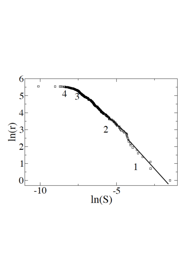
Figure 1: .

After visual inspection and much statistical analysis of the data, i.e., adapting the limits of the relevant intervals by trial and error procedures, it is found that the cities are best grouped into four classes: large cities (class 1); medium size cities (class 2); small cities (class 3) and very small cities (class 4). A comment on the various sizes has to be found below, after the data specific analysis. Fig. 1 outlines the rank-size relationship for the rescaled sizes $S$ of the system of Bulgarian cities, in 2004. The figures for other analyzed years, 2005-2011, are not shown, for conciseness, but are very similar to the 2004 case.

2004
[Pop]	$N_{c}$	Cl.	$\alpha$	$\beta$	$\gamma$
1.14 106	16	1	$-1.79\pm 0.19$	$0.99\pm 0.05$	-
70 000	122	2	$-0.77\pm 0.03$	$0.820\pm 0.004$	-
5 000	93	3	$-20.99\pm 0.14$	$6.47\pm 0.21$	$0.39\pm 0.02$
2 000	17	4	$4.42\pm 0.06$	$0.128\pm 0.007$	-
2011
[Pop]	$N_{c}$	Cl.	$\alpha$	$\beta$	$\gamma$
1.21 106	15	1	$-1.46\pm 0.18$	$0.89\pm 0.06$	-
70 000	120	2	$-0.910\pm 0.002$	$0.837\pm 0.004$	-
5 000	94	3	$-23.94\pm 0.19$	$7.16\pm 0.24$	$0.43\pm 0.03$
2 000	28	4	$3.82\pm 0.07$	$0.204\pm 0.008$	-

Table 1: Values of the parameters $\alpha$, $\beta$, and $\gamma$ for the four classes of Bulgarian cities for 2004 and 2011; see Eqs.(3)-(4). The number of cities in each Class (Cl.) is given together with the respective population upper size ([Pop]) in the Class.

It is found that the rank-size relationship for the classes 1, 2, and 4 can be approximated by a straight line (Zipf’s law), Eq.(3). The parameters $\alpha$ and $\beta$ for these classes are given in Table 1. Note that for the case of large cities the exponent $\beta$ is almost $1$, as conjectured by Zipf to be an optimal case. In contrast, the rank-size relationship for the small cities in class 3 is very well approximated by a $quadratic$ regression of the kind

$$\ln(r)=\alpha-\beta\ln(S)-\gamma(\ln(S))^{2},$$ (4)

where the corresponding parameters are written in Table 1. For comparison, the parameters for the rank-size distribution of the Bulgarian cities for 2011 are also given in Table 1.

For completeness, the number of cities and their population ranges in each class are given in Table 1. We emphasize that the grouping is not made a priori but results from data analysis. The fact that the analysis of unbiased measurement yields consistent results over time allows us to state that the prediction can be said to be reliable.

We only show 2004 and 2011, but indicate in the text, that these are only examples which are confirmed in other years. On the basis of above we have reliability of the hypothesis for the entire studied interval from 2004 till 2011. This grouping is not unusual as such a separation into classes was observed also for the case of other countries, cf., e.g., (Davis (1978); Rubinstein (2007)).

Thus, Fig. 1 and Table 1 indicate that Hypothesis 1 is not valid for the Bulgarian city system.

Let us supply some more argument for such a conclusion, e.g. through a Pareto plot (Pareto (1896); Reed (2001); Reed and Jorgensen (2004)), i.e. let it be searched whether the cumulative distribution function of such a population system follows an inverse power law of $S$.

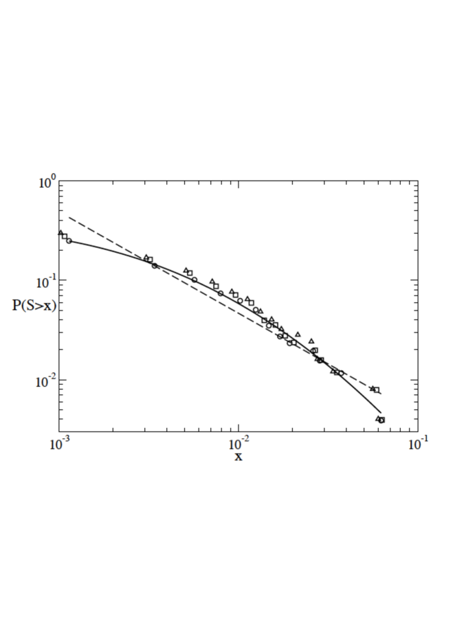
Figure 2:

The theory of the size-independent growth predicts a power law for $P(S>x)\sim S^{-\zeta}$, with a constant $\zeta$. The probability $P(S>x)$ that the rescaled size of a Bulgarian city population exceeds a certain value $x$ in 2011 is shown in Fig. 2. In Fig. 2, this theory is represented by the dashed line, i.e. a power law fit to the data. It is easily seen that a power law is not a good approximation for the (rescaled) city population size distribution in Bulgaria. An extended version of the theory of the city growth should allow for a population size dependent growth. As a consequence of this, the exponent $\zeta$ depends on the population size of the city. Therefore, some $\zeta(x)$ can be estimated as follows.

The solid line in Fig. 2 represents the fit of the probability $P(S>x)$ for the system of Bulgarian cities for 2011. This fit corresponds to the distribution

$$P(x)=\frac{a}{2}{\rm erfc}\left[-\frac{\ln(x/b)}{c\sqrt{2}}\right]$$ (5)

where $a$, $b$ and $c$ are parameters and ${\rm erfc}(x)=1-{\rm erf(x)}$ where ${\rm erf(x)}$ is

$${\rm erf}(x)=\frac{2}{\sqrt{\pi}}\int_{0}^{x}dy\ e^{-y^{2}}.$$ (6)

In order to obtain $\zeta(x)$, the theoretical distribution $(x/S_{min})^{-\zeta(x)}$ is assumed to be the same as Eq.(5), i.e.,

$$\left(\frac{x}{S_{min}}\right)^{-\zeta(x)}=\frac{a}{2}{\rm erfc}\left[-\frac{\ln(x/b)}{c\sqrt{2}}\right].$$ (7)

From Eq.(7), the $local$ exponent $\zeta(x)$ is so obtained:

$$\zeta(x)=-\frac{\ln(a/2)+\ln\{{\rm erfc}[-(\ln(x/b))/(c\sqrt{2})]\}}{\ln(x/S_{min})}.$$ (8)

The local exponent from Eq.(8) is shown in Fig. 3.

Figure 3:

For a large interval of $x$ the value of $\zeta$ is close to $1$, the Zipf value. Large deviations from $1$ are observed for the class of small cities. If Hypothesis 1 was true for the whole system of Bulgarian cities, $\zeta$ should be a constant corresponding to a straight line in Fig. 3. This is not the case,thereby implying that Hypothesis 1 is not valid for the system of Bulgarian cities.

3 Test of Hypothesis 2

It is emphasized first that the Hypothesis 2 is formulated for the non-rescaled sizes of the populations in a system of cities. The test of the hypothesis goes as follows: the city population size distribution for the Bulgarian cities is fitted to the double Pareto log-normal distribution,

$$p(x)=\frac{\alpha\beta}{2(\alpha+\beta)}\exp\left(\alpha\mu+\frac{\alpha^{2}\sigma^{2}}{2}\right)x^{-\alpha-1}\left[1+{\rm erf}\left(\frac{\ln(x)-\mu-\alpha\sigma^{2}}{\sigma\sqrt{2}}\right)\right]+$$

$$\frac{\alpha\beta}{2(\alpha+\beta)}\exp\left(-\beta\mu+\frac{\beta^{2}\sigma^{2}}{2}\right)x^{\beta-1}\left[1-{\rm erf}\left(\frac{\ln(x)-\mu+\beta\sigma^{2}}{\sigma\sqrt{2}}\right)\right]$$

If the assumptions of Hypothesis 2 are correct, it should be expected that the double Pareto log-normal distribution provides a good fit to the data. However, if one or more of the assumptions in Hypothesis 2 are not valid, the fit should not be a satisfactory one.

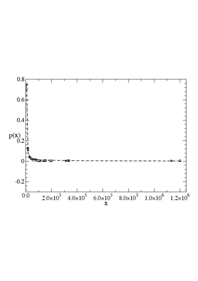
Figure 4:

.

The distribution of population sizes of the system of Bulgarian cities in 2004 and in 2011 are presented in Fig. 4. The dash line represents the double Pareto log-normal distribution that corresponds to the distribution of the Bulgarian cities in 2011. From the values of $\alpha$ and $\beta$ and from the properties of the double Pareto log-normal distribution it follows that $p(x)\approx x^{-0.8}$ , for the case of small city sizes and $p(x)\approx x^{-3}$ for the large cities. Similar results are found for the years for which the data are available.

Thus, the double Pareto log-normal distribution fits well the city population size distributions for the Bulgarian city system whatever the year in this century. Thus Hypothesis 2 is confirmed.

4 Concluding remarks

The study of the size of populations in cities of a country has many economic applications. Apart on the decision taking about placing industrial plants or building trade centers, the city population sizes influence the efficient use of resources or the possibilities of economic growth (Henderson (1986, 2001)). Thus, the investigation of the evolution of the populations in a system of cities is an important research topic.

Our study reported here above has shown that for the case of the Bulgarian city system Hypothesis 1 is not confirmed but Hypothesis 2 is confirmed. The validity of Hypothesis 2 even gives some information about the history of settlement formations in Bulgaria. It seems that the distribution of the initial populations of the settlements was indeed log-normal and that the formation happened according to the Yule process, i.e. the new settlements have been formed on the basis of the existing older settlements nearby.

Acknowledgment

This work has been performed in the framework of COST Action IS1104 ”The EU in the new economic complex geography: models, tools and policy evaluation”. We acknowledge some support through the project ’Evolution spatiale et temporelle d’infrastructures régionales et économiques en Bulgarie et en Fédération Wallonie-Bruxelles’ within the intergovernmental agreement for cooperation between the Republic of Bulgaria and la Communauté Française de Belgique.

Supplemental material

Supplemental material can be found containing some brief review of the pertinent literature on nonlinear dynamics, nonlinear time series analysis and their applications. The two hypotheses tested in the main text of the paper being closely connected to the existence of power laws for the population sizes of the cities are discussed along analytical lines. It is shown that Kesten and Gibrat proportional random growth processes lead to power law distributions. On the other hand, the Yule process of settlement formation and the geometric Brownian motion assumed for their growth is shown to result in a double Pareto log-normal distribution.

Fig. 1 Rank-size relationship for the system of Bulgarian cities in 2004. The cities are divided into 4 classes. The rank-size relationships for the classes 1, 2, and 4 are fitted by a linear regression $\ln(r)=\alpha-\beta\ln(S)$.

Fig. 2 Probability $P(S>x)$ that the rescaled population city size $S_{i}$ of Bulgarian cities is larger than some value $x$ in 2004 (triangles), 2007 (squares), and 2011 (circles). Dashed line: Power law distribution with a constant exponent $\zeta=1.02$. Solid line: Eq.(5) with $a=0.359$; $b=0.0023$; $c=-1.469$.

Fig. 3 Local exponent $\zeta(x)$ from Eq.(8) with parameter values of Fig.2. The vertical lines mark the boundaries between the 4 classes of cities from large to small sizes with increasing $x$.

Fig. 4 Probability density functions for Bulgarian city population size in 2004 (circles) and 2011 (squares) with a double Pareto log-normal distribution fit Eq.(3) (dashed line) for 2011. The parameters of the double Pareto log-normal distribution from the dashed line are: $\alpha=2.049$; $\beta=0.216$, $\sigma=-6.188$; $\mu=-25.737$. $R^{2}=0.996$ in 2011.

References

- Cordoba (2008a) Córdoba J.-C., 2008a. On the distribution of city sizes. Journal of Urban Economics 63, 177-197.
- Cordoba (2008b) Córdoba, J.-C., 2008b. A generalized Gibrat’s Law. International Economic Review 49, 1463-1468.
- Davis (1978) Davis K., 1978. World urbanization: 1950-1970, in: Bourne I.S., Simons J.W. (Eds.), Systems of Cities. Oxford University Press, New York, pp. 92-100.
- Gangopadyay and Basu (2009) Gangopadyay K., Basu B., 2009. City size distributions for India and China. Physica A 398, 2682-2688.
- Glaeser (2008) Glaeser E.L., 2008. Cities, agglomeration and spatial equilibrium. Oxford University Press, New York.
- Henderson (1986) Henderson J.V., 1986. Efficiency of resource usage and city size. J. Urban. Economics 19, 47-70.
- Henderson (2001) Henderson J.V., Shalizi Z., Venables A.J., 2001. Geography and development. J. Econ. Geography 1, 81-105.
- Ioannides and Overman (2003) Ioannides Y.M., Overman H.G., 2003. Zipf’s law for cities: an empirical examination. Regional Science and Urban Economics 33, 127-137.
- Jiang and Tia (2011) Jiang B., Tia J., 2011. Zipf’s law for all the natural cities in the United States: a geospatial perspective. Int. J. Geogr. Inf. Sci. 25, 1269 - 1281.
- Knudsen (2001) Knudsen T., 2004. Zipf’s law for cities and beyond: The case of Denmark. Am. J. Econ. Soc. 60, 123-146.
- Krugman (1996) Krugman P., 1996. Confronting the mistery of urban hierarchy. Journal of Japanese and International Economics 10, 399-418.
- Madden (1956) Madden C.H., 1956. Some Temporal Aspects of the Growth of Cities in the United States. Economic Development and Cultural Change 4, 236-252.
- Moura (2006) Moura N.J. Jr., Ribeiro M.B. 2006. Zipf law for Brasilian cities. Physica A 367, 441-448.
- Newman (2005) Newman M.E.J., 2005. Power laws, Pareto distributions and Zipf’s law. Contemporary Physics 46, 323-351.
- Pareto (1896) Pareto V., 1896. Cours d’Economie Politique Droz, Geneva, Switzerland.
- Peng (2010) Peng C.-H. 2010. Zipf’s law for Chinese cities: rolling sample regressions. Physica A 389, 3804-3813.
- Puu and Panchuk (1991) Puu T., Panchuk A., 1991. Nonlinear economic dynamics. Springer, Berlin.
- Reed (2001) Reed W.J., 2001. The Pareto, Zipf and other power laws. Economics Letters 74, 15-19.
- Reed and Jorgensen (2004) Reed W.J., Jorgensen M., 2004. The double Pareto-log-normal distribution: a new parametric model for size distributions. Communications in Statistics-Theory and Methods 33, 1733-1753.
- Rubinstein (2007) Rubenstein J.M., 2007. The Cultural Landscape: An Introduction to Human Geography, ninth ed. Prentice Hall, Englewood Cliffs, NJ.
- Seto and Fragkias (2005) Seto K.C., Fragkias M., 2005. Quantifying spatiotemporal patterns of urban land-use change in four cities of China with time series landscape metrics. Landscape Ecology 20, 871-888.
- Sheppard (1982) Sheppard E., 1982. City size distributions and spatial economic change. WP-82-31, Working papers of the International Institute for Applied System Analysis, Laxenburg, Austria.
- Vespignani (2009) Vespignani A., 2009. Predicting the behavior of techno-social systems. Science 325, 425-428.
- Vitanov et al. (2007) Vitanov N.K., Sakai K., Jordanov I.P., Managi S., Demura K., 2007. Analysis of a Japan government intervention on the domestic agriculture market. Physica A 382, 330-335.
- Zipf (1949) Zipf G.K., 1949. Human Behavior and the Principle of Least Effort : An Introduction to Human Ecology. Addison Wesley, Cambridge, Mass.