Two-dimensional Turbulence in Symmetric Binary-Fluid Mixtures: Coarsening Arrest by the Inverse Cascade

Abstract

We study two-dimensional (2D) binary-fluid turbulence by carrying out an extensive direct numerical simulation (DNS) of the forced, statistically steady turbulence in the coupled Cahn-Hilliard and Navier-Stokes equations. In the absence of any coupling, we choose parameters that lead (a) to spinodal decomposition and domain growth, which is characterized by the spatiotemporal evolution of the Cahn-Hilliard order parameter $\phi$, and (b) the formation of an inverse-energy-cascade regime in the energy spectrum $E(k)$, in which energy cascades towards wave numbers $k$ that are smaller than the energy-injection scale $k_{inj}$ in the turbulent fluid. We show that the Cahn-Hilliard-Navier-Stokes coupling leads to an arrest of phase separation at a length scale $L_{c}$, which we evaluate from $S(k)$, the spectrum of the fluctuations of $\phi$. We demonstrate that (a) $L_{c}\sim L_{H}$, the Hinze scale that follows from balancing inertial and interfacial-tension forces, and (b) $L_{c}$ is independent, within error bars, of the diffusivity $D$. We elucidate how this coupling modifies $E(k)$ by blocking the inverse energy cascade at a wavenumber $k_{c}$, which we show is $\simeq 2\pi/L_{c}$. We compare our work with earlier studies of this problem.

Two-dimensional (2D) fluid turbulence, which is of central importance in a variety of oceanographic and atmospheric flows, is fundamentally different from three-dimensional (3D) fluid turbulence as noted in the pioneering studies of Fjørtoft, Kraichnan, Leith, and Batchelor fjo53 ; kra67 ; lei68 ; bat69 ; Les97 . In particular, the fluid-energy spectrum in 2D turbulence shows (a) a forward cascade of enstrophy (or the mean-square vorticity), from the energy-injection wave number $k_{inj}$ to larger wave numbers, and (b) an inverse cascade of energy to wave numbers smaller than $k_{inj}$. We elucidate the arrest of phase separation in a 2D, symmetric, binary-fluid mixture by turbulence.

In the absence of turbulence, binary-fluid mixtures have played a pivotal role in the development of the understanding of (a) equilibrium critical phenomena at the consolute point, above which the two fluids mix fish67 ; kum83 ; Kar07 , (b) of nucleation hua74 , and (c) spinodal decomposition, the process by which a binary-fluid mixture, below the consolute point and below the spinodal curve, separates into the two, constituent liquid phases until, in equilibrium, a single interface separates the two coexisting phases gun83 ; onu02 . In the late stages of growth, as the binary-fluid mixture evolves via spinodal decomposition towards the completely phase-separated, equilibrium state, the domains of these two phases coarsen to yield ever larger domains whose linear size diverges as a power of the time $t$; this divergence leads to universal scaling forms for the time-dependent correlation functions lif59 ; fur85 ; sig79 ; bra94 ; wag98 ; ken00 ; ken01 ; onu02 ; puri09 ; cat12 ; datt15 of the order parameter $\phi$, which distinguishes the two phases of the binary-fluid mixture.

Coarsening arrest by 2D turbulence has been studied in Ref. ber05 , where it has been shown that, for length scales smaller than the energy-injection scale $\ell_{inj}=2\pi/k_{inj}$, the typical linear size of domains is controlled by the average shear across the domain. However, the nature of coarsening arrest, for scales larger than $\ell_{inj}$, i.e., in the inverse-cascade regime, still remains elusive. In particular, it is not clear what happens to the inverse energy transfer, in a 2D binary-liquid, turbulent mixture, in which the mean size of domains provides an additional, important length scale. We resolve these two issues in our study. By combining theoretical arguments with extensive direct numerical simulations (DNSs) we show that the Hinze length scale $L_{H}$ (see Refs. per14 ; hin55 ) provides a natural estimate for the arrest scale; and the inverse flux of energy also stops at a wave-number scale $\simeq 2\pi/L_{H}$. In particular, we study two-dimensional (2D) binary-fluid turbulence by carrying out a direct numerical simulation (DNS) of the forced, statistically steady turbulence in the coupled Cahn-Hilliard and Navier-Stokes equations. In the absence of any coupling, our choice of forcing leads (a) to spinodal decomposition and domain growth, which we examine by the spatiotemporal evolution of $\phi$, and (b) to the formation of an inverse-energy-cascade regime in the energy spectrum $E(k)$, in which energy cascades towards wave numbers $k$ that are smaller than the energy-injection scale $k_{inj}$ in the turbulent fluid. We show that the Cahn-Hilliard-Navier-Stokes coupling leads to an arrest of phase separation at a length scale $L_{c}$, which we evaluate from $S(k)$, the spectrum of the fluctuations of $\phi$. We demonstrate (a) $L_{c}\sim L_{H}$ and (b) that $L_{c}$ is independent, within error bars, of the diffusivity $D$. We elucidate how this coupling modifies $E(k)$ by blocking the inverse energy cascade at a wavenumber $k_{c}$, which we show is $\simeq 2\pi/L_{c}$.

We model a symmetric binary-fluid mixture by using the incompressible Navier-Stokes equations coupled to the Cahn-Hilliard or Model-H equations hoh77 ; cah68 . We are interested in 2D incompressible fluids, so we use the following stream-function-vorticity formulation per09 ; per09b ; bof12 for the momentum equation:

$$(\partial_{t}+\bm{u}\cdot\nabla)\omega = \nu\nabla^{2}\omega-\nabla\times(\phi\nabla\mu)+f_{\omega},$$ (1)

$$(\partial_{t}+{\bm{u}}\cdot\nabla){\phi} = M\nabla^{2}{\mu},~{}{\rm{and}}~{}\nabla\cdot{\bm{u}}=0.$$ (2)

Here ${\bm{u}}\equiv(u_{x},u_{y})$ is the fluid velocity, $\omega=(\nabla\times{\bm{u}}){\hat{\bm{e}}}_{z}$, $\phi({\bm{x}},t)\in[-1,1]$ is the Cahn-Hilliard order parameter at the point ${\bm{x}}$ and time $t$, $p$ is the pressure, $\mu({\bm{x}},t)=\delta{\mathcal{F}}[\phi]/\delta\phi({\bm{x}},t)$ is the chemical potential, ${\mathcal{F}}[\phi]=\Lambda\int[(\phi^{2}-1)^{2}/(4\xi^{2})+|\nabla\phi|^{2}/2]d{\bm{x}}$ is the free energy, $\Lambda$ is the mixing energy density, $\xi$ controls the width of the interface between the two phases of the binary-fluid mixture, $\nu$ is the kinematic viscosity, the surface tension $\sigma=2\sqrt{2}/3(\Lambda/\xi)$, the mobility of the binary-fluid mixture is $M$, and $f_{\omega}$ is the external driving force. For simplicity, we study mixtures in which $M$ is independent of $\phi$ and both components have the same density and viscosity ken01 . We use periodic boundary conditions in our square simulation domain, with each side of length $L=2\pi$. To obtain a substantial inverse-cascade regime, we stir the fluid at an intermediate length scale by forcing in Fourier space in a spherical shell with wave-number $k_{inj}=2\pi/\ell_{inj}$. Our choice of forcing $\hat{f}_{\omega}({\mathbf{k}},t)=\hat{\omega}({\mathbf{k}},t)/\sum_{k=k_{inj}}\hat{\omega}({\mathbf{k}},t)$, where the caret indicates a spatial Fourier transform, ensures that there is a constant enstrophy-injection rate. In all our studies we use $k_{inj}=40$ so that there is a clear separation between $\ell_{inj}$ and $\xi$. We conduct DNSs of Eqs. (1) and (2) by using a pseudospectral method Can88 ; because of the cubic nonlinearity in the chemical potential $\mu$, we use $N/2$-dealiasing. For time integration we use the exponential Adams-Bashforth method ETD2 cox02 . Important nondimensional numbers for the turbulent flows here are the Grashof number $Gr\equiv(L^{4}f_{\omega}/\nu^{2})$, the injection-scale Reynolds number $Re\equiv u_{inj}\ell_{inj}/\nu$, with $u_{inj}=(\epsilon_{inj}\ell_{inj})^{1/3}$, where $\epsilon_{inj}$ is the energy-injection rate, the Weber number $We\equiv\rho u_{inj}^{2}\ell_{inj}/\sigma$, the Cahn number $Ch=\xi/L$, the Peclet number $Pe\equiv u_{rms}L/D$, where $u_{rms}$ is the root-mean square velocity, and the Schmidt number $Sc\equiv\nu/D$, where $D\equiv M\Lambda/\xi^{2}$ is the diffusivity of our binary-fluid mixture. We give the parameters for our simulations in the Supplemental Material suppmat .

Given ${\bm{u}}({\bm{x}},t)$ and $\phi({\bm{x}},t)$ from our DNS, we calculate the energy and order-parameter (or phase-field) spectra, which are, respectively, $E(k)\equiv\sum_{k-\frac{1}{2}\leq k^{\prime}\leq k+\frac{1}{2}}\langle|\hat{\bm{u}}({\mathbf{k}}^{\prime},t)|^{2}\rangle_{t}$ and $S(k)\equiv\sum_{k-\frac{1}{2}\leq k^{\prime}\leq k+\frac{1}{2}}\langle|\hat{\phi}({\mathbf{k}}^{\prime},t)|^{2}\rangle_{t}$, where $\langle\rangle_{t}$ denotes the average over time in the statistically steady state of our system. The total kinetic energy is $E(t)=\frac{1}{2}\langle|{\bf u}({\bm{x}},t)|^{2}\rangle_{{\bm{x}}}$ and the total enstrophy $\epsilon(t)=\frac{1}{2}\langle|\omega({\bf x},t)|^{2}\rangle_{{\bf x}}$, where $\langle\rangle_{{\bm{x}}}$ denotes the average over space, $\langle f_{\omega}\omega\rangle$ is the enstrophy-injection rate, which is related to the energy-injection rate via $\epsilon_{inj}=\langle f_{\omega}\omega\rangle/k_{inj}^{2}$, $E=0.5\sum_{k}E(k)$ is the fluid kinetic energy, $\epsilon_{\nu}=\nu\sum_{k}k^{2}E(k)$ is the fluid-energy dissipation rate, and $\epsilon_{\mu}=M\sum_{k}k^{2}\langle|\hat{\mu}({\mathbf{k}},t)|^{2}|\rangle_{t}$ is the energy-dissipation rate because of the phase field $\phi$.

Forced, 2D, statistically steady, Navier-Stokes-fluid turbulence displays a forward cascade of enstrophy, from $\ell_{inj}$ to smaller length scales, and an inverse cascade of energy to length scales smaller than $\ell_{inj}$. In the inverse-cascade regime, on which we concentrate here, $E(k)\sim k^{-5/3}$ (see, e.g., Refs. kra67 ; Les97 ) and the energy flux $\Pi(k)\sim\epsilon\equiv\langle\epsilon(t)\rangle_{t}$ assumes a constant value. For the Cahn-Hilliard model, if it is not coupled to the Navier-Stokes equation, $S(k,t)\sim{\mathcal{S}}(k\mathbb{L}(t))$, for large times, where the time-dependent length scale $\mathbb{L}(t)\sim t^{1/3}$, in the early Lifshitz-Slyozov lif59 ; bra94 ; puri09 ; cat12 regime; if the Cahn-Hilliard model is coupled to the Navier-Stokes equation, then, in the absence of forcing, $\mathbb{L}(t)\sim t$, in the viscous-hydrodynamic regime, first discussed by Siggia sig79 ; bra94 ; puri09 ; cat12 , and $\mathbb{L}(t)\sim t^{2/3}$, in the very-late-stages in the Furukawa fur85 and Kendon ken00 regimes. For a discussion of these regimes and a detailed exploration of a universal scaling form for $\mathbb{L}(t)$ in 3D we refer the reader to Ref. ken01 . We now elucidate how these scaling forms for $E(k)$ and $S(k,t)$ are modified when we study forced 2D turbulence, in the inverse-cascade regime in the coupled Cahn-Hilliard-Navier-Stokes equations.

In Fig. 1 we show pseudo-gray-scale plots of $\phi$, at late times when coarsening arrest has occurred, for four different values of $We$ at $Re=124$; we find that the larger the value of $We$ the smaller is the linear size that can be associated with domains; this size is determined by the competition between turbulence-shear and interfacial-tension forces. This qualitative effect has also been observed in earlier studies of 2D and 3D turbulence of symmetric binary-fluid mixtures cha87 ; rui81 ; pine84 ; aro84 ; has95 ; lac95 ; onu97 ; berth01 ; ber05 .

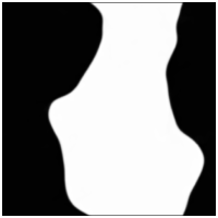
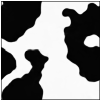
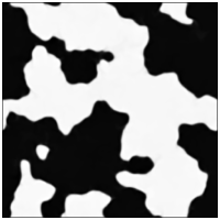
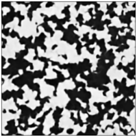
Figure 1: Pseudo-gray-scale plots of the order parameter field $\phi$, at late times when coarsening arrest has occured, in 2D symmetric-binary-fluid turbulence with $Re=124$. Note that the domain size decreases as we increase the Weber number $We$ from the leftmost to the rightmost panel: $We=1.2\cdot 10^{-2}$ (${\tt R3}$); $We=5.9\cdot 10^{-2}$ (${\tt R4}$); $We=1.2\cdot 10^{-1}$ (${\tt R5}$); and $We=5.9\cdot 10^{-1}$ (${\tt R8}$).

We calculate the coarsening-arrest length scale

$$L_{c}=2\pi[\sum_{k}S(k)]/[\sum_{k}kS(k)].$$ (3)

We now show that $L_{c}$ is determined by the Hinze scale $L_{H}$, which we obtain, as in Hinze’s pioneering study of droplet break-up hin55 , by balancing the surface tension with the inertia as follows:

$$L_{H}\sim\epsilon_{inj}^{-2/5}\sigma^{3/5}.$$ (4)

We obtain for 2D, binary-fluid turbulence the intuitively appealing result $L_{c}\sim L_{H}$ (for a similar, recent Lattice-Boltzmann study in 3D see Ref. per14 ). In particular, if we determine $L_{c}$ from Eq. (3), with $S(k)$ from our DNS, we obtain the red points in Fig. 2, which is a log-log plot of $\sigma L_{c}$ versus $\epsilon_{inj}/\sigma^{4}$; the black line is the Hinze result (4) for $L_{H}$, with a constant of proportionality that we find is $\simeq 1.6$ from a fit to our data. We see from Fig. 2 that the Hinze length scale $L_{H}$ gives an excellent approximation to the arrest scale $L_{c}$ over several orders of magnitude on both vertical and horizontal axes. Note that the Hinze estimate also predicts that, for fixed values of $\epsilon_{inj}$ and $\sigma$, the coarsening-arrest scale is independent of $D$; the plot of $L_{c}$ versus $D$, in the inset of Fig. 2, shows that our data for $L_{c}$ are consistent (within error bars) with this prediction.

In Fig. 2 (b) we show clearly how the arrest of coarsening manifests itself as a suppression of $S(k)$, at small $k$ (large length scales). This suppression increases as $We$ increases (i.e., $\sigma$ decreases); and $S(k)$ develops a broad and gentle maximum whose peak moves out to large values of $k$ as $We$ grows. These changes in $S(k)$ are associated with $We$-dependent modifications in the probability distribution function (PDF) $P(\phi)$ of the order parameter $\phi$, which is symmetrical about $\phi=0$ and has two peaks at $\phi=\phi_{\pm}$, where $\phi_{+}=-\phi_{-}>0$; we display $P(\phi)/P_{m}(\phi)$ in Fig. 2 (c) in the vicinity of the peak at $\phi_{+}$; as $We$ increases, $\phi_{+}$ decreases; here $P_{m}(\phi)$ is the maximum value of $P(\phi)$. In particular, our DNS suggests that $1-\phi_{+}^{2}\sim We^{1/2}$, for small $We$.

The modification in $P(\phi)$ can be understood qualitatively by making the approximation that the effect of the fluid on the equation for $\phi$ can be encapsulated into an eddy diffusivity $D_{e}$ aro84 ; nar07 . The eddy-diffusivity-modified Cahn-Hilliard equation is $\partial_{t}\phi=(D_{e}-D)\nabla^{2}\phi+D\nabla^{2}\phi^{3}+M\Lambda\nabla^{4}\phi$, which gives the maximum and minimum values of $\phi$ as $\phi_{\pm}=\sqrt{(D-D_{e})/D}$. Furthermore, if we neglect the nonlinear term bra94 ; cat12 , we find easily that the modified growth rate is $Dk^{2}[(1-D_{e}/D)-M\Lambda k^{2}]$; i.e., all wave numbers larger than $k_{d}=\sqrt{(1-D_{e}/D)/(\Lambda M)}$ are stable to perturbations. In particular, droplets with linear size $<$($2\pi/k_{d}$) decay in the presence of coupling with the velocity field; we expect, therefore, that, in the presence of fluid turbulence, the peak of $P(\phi)$ broadens and shifts as it does in our DNS. For a quantitative description of this broadening and the shift of the peak, we must, of course, carry out a full DNS of the Cahn-Hilliard-Navier-Stokes equation as we have done here.

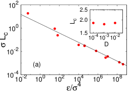
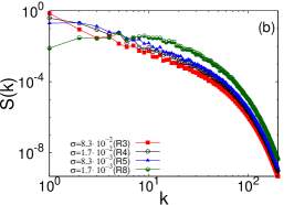
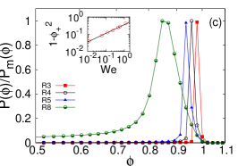
Figure 2: (Color online)(a) Log-log (base 10) plot of $\sigma L_{c}$ versus $\epsilon/\sigma^{4}$ showing data points ($L_{c}$ from Eq. (3), with $S(k)$ from our DNS) in red. The black line is the Hinze result (4) for $L_{H}$; a fit to our data yields a constant of proportionality $\simeq 1.6$ and an excellent approximation to the arrest scale $L_{c}$ over several orders of magnitude on both vertical and horizontal axes; the plot of $L_{c}$ versus $D$, in the inset, shows that, for fixed values of $\epsilon_{\nu}$ and $\sigma$ (runs R1,R2 and R4), $L_{c}$ is independent of $D$ (within error bars), as is implied by the Hinze condition (see text). (b) Log-log (base 10) plots of the spectrum $S(k)$, of the phase-field $\phi$, versus $k$; as $We$ increases (i.e., $\sigma$ decreases) the low-$k$ part of $S(k)$ decreases and $S(k)$ develops a broad and gentle maximum whose peak moves out to large values of $k$. (c) Plots versus $\phi$, in the vicinity of the maximum at $\phi_{+}$, of the normalized PDFs $P(\phi)/P_{m}(\phi)$, where $P_{m}(\phi)$ is the maximum of $P(\phi)$; the peak position $\phi_{+}\to 1$ as $We$ increases (see the inset which suggests that $1-\phi_{+}^{2}\sim We^{1/2}$ (black line)).

We have investigated, so far, the effect of fluid turbulence on the phase-field $\phi$ and its statistical properties such as those embodied in $S(k)$ and $P(\phi)$. We show next how the turbulence of the fluid is modified by $\phi$, which is an active scalar insofar as it affects the velocity field. In the statistically steady state of our driven, dissipative system, the energy injection must be balanced by both viscous dissipation and dissipation that arises because of the interface, i.e., we must have $\epsilon_{inj}=\epsilon_{\nu}+\epsilon_{\mu}$.

In Fig. 3(a), we show that $\epsilon_{\nu}$ decreases and $\epsilon_{\mu}$ increases as we increase $We$, while keeping $\epsilon_{inj}$ constant, because $L_{c}$ diminishes (Fig. 1) and, therefore, the interfacial length and $\epsilon_{\mu}$ increase. This decrease of $L_{c}$ is mirrored strikingly in plots of the fluid-kinetic-energy spectrum $E(k)$ (Fig. 3(b)), which demonstrate that the inverse cascade of energy is effectively blocked at a wavenumber $k_{c}$, which we determine below, from the energy flux, and which we find is $\simeq 2\pi/L_{c}$, where $L_{c}$ follows from $S(k)$ (see Fig. 2). The value of $k_{c}$ increases with $We$; and the inverse cascade is completely blocked for the largest $We$ we use, for which $k_{c}\simeq k_{inj}$, the forcing scale.

To provide clear evidence that the blocking of the energy flux is closely related to the arrest scale, we show in Fig. 3(c) plots of the energy flux $\Pi_{E}(k)=\int_{k}^{\infty}T(k^{\prime})dk^{\prime}$ for different values of $We$. Here $T(k)=\sum_{k-\frac{1}{2}\leq k^{\prime}\leq k+\frac{1}{2}}\langle\hat{\bm{u}}(-{\mathbf{k}},t)\cdot{\bf P}({\bf k})\cdot\widehat{({\bm{u}}\times{\bm{\omega}})({\bf k},t)}\rangle_{t}$ is the energy transfer and ${\bf P}({\bf k})$ is the transverse projector with components $P_{ij}(k)\equiv\delta_{ij}-k_{i}k_{j}/k^{2}$. We define $k_{c}$ as the wave-number at which $\Pi_{E}(k)$ becomes $4\%$ of $\epsilon_{inj}$. We find that the wave-numer corresponding to the arrest scale $2\pi/L_{c}$ (marked by vertical lines for each run) is comparable to $k_{c}$.

It has been suggested ber01 ; nar07 that coarsening arrest can be studied by using a model in which the field $\phi$ is advected passively by the fluid velocity. Such a passive-advection model is clearly inadequate because it cannot lead to the phase-field-induced modifications in the statistical properties of the turbulent fluid (see Fig. 3). However, for the sake of completeness, we now study the passive-advection case in which the coupling term $\phi\nabla\mu$ is turned off in Eq. (2). We then contrast the results for this case with the ones we have presented above. The parameters we use for the passive-advection DNS are $N=1024,\Lambda=\xi^{2},\xi=0.0176$; and we carry out runs for $D=5\cdot 10^{-3},1\cdot 10^{-2},5\cdot 10^{-2}$ and $5\cdot 10^{-1}$. The evolution of the pseudo-grayscale plots of $\phi$ with $D$, in the left panel of Fig. 4, is qualitatively similar to the evolution shown in Fig. 1. There is also a qualitative similarity in the dependence on $D$ of the scaled PDFs $P(\phi)/P_{m}(\phi)$; we can see this by comparing the passive-advection result, shown in the middle panel of Fig. 4 for positive values of $\phi$ in the vicinity of the peak, with its counterpart in Fig. 2 (c). However, there is a qualitative difference in the dependence of $L_{c}$ on $D$: in the passive-advection case we find $L_{c}\sim D^{0.27}$ [Fig. 4 (inset)], which is in stark contrast to the essentially $D$-independent behavior of $L_{c}$ shown in the inset of Fig. 2(c).

In conclusion, our extensive study of two-dimensional (2D) binary-fluid turbulence shows how the Cahn-Hilliard-Navier-Stokes coupling leads to an arrest of phase separation at a length scale $L_{c}$, which follows from $S(k)$. We demonstrate that $L_{c}\sim L_{H}$, the Hinze scale that we find by balancing inertial and interfacial-tension forces, and that $L_{c}$ is independent, within error bars, of the diffusivity $D$. We also elucidate how the coupling between the Cahn-Hilliard and Navier-Stokes equations modifies the properties of fluid turbulence in 2D. In particular, we show that there is a blocking of the inverse energy cascade at a wavenumber $k_{c}$, which we show is $\simeq 2\pi/L_{c}$.

Earlier DNSs of turbulence-induced coarsening arrest in binary-fluid phase separation have concentrated on regimes in which there is a forward cascade of energy in 3D (see Ref. per14 ) and a forward cascade of enstrophy in 2D (see Ref. ber05 ). Although studies that use a passive-advection model for $\phi$ obtain results that are qualitatively similar to those we obtain for $S(k)$ and the spatiotemporal evolution of $\phi$, they cannot capture the phase-field-induced modification of the statistical properties of fluid turbulence and the correct dependence of $L_{c}$ on $D$. We find our results to be in qualitative agreement with the earlier studies on advection of binary-fluid mixtures with synthetic chaotic flows nar07 ; of course, such studies cannot address the effect of the phase field on the turbulence in the binary fluid.

Some groups have also studied the statistical properties of turbulent, symmetric, binary-fluid mixtures above the consolute point, where the two fluids mix even in absence of turbulence rui81 ; jen98 . In these studies, there is, of course, neither coarsening nor coarsening arrest.

We hope our study will lead to new experimental studies of turbulence in binary-fluid mixtures, especially in 2D muz91 ; sol96 , to test the specific predictions we make for $L_{c}$ and the blocking of the inverse cascade of energy.

We thank S.S. Ray for discussions, the Department of Atomic Energy, the Department of Science and Technology, Council for Scientific and Industrial Research, and the University Grants Commision (India) for support.

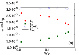
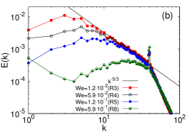
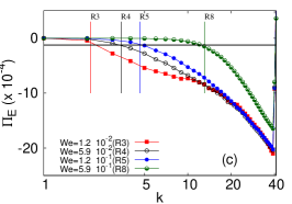
Figure 3: (Color online) (a) Plots of the statistically-steady-state values of $\epsilon_{\nu}$, $\epsilon_{\mu}$, and their sum $\epsilon_{\nu}+\epsilon_{\mu}\simeq\epsilon_{inj}$ versus $We$. (b) Log-log (base $10$) plots of the energy spectrum $E(k)$ versus $k$, for different values of $We$, illustrating the truncation of the inverse energy cascade as $We$ increases. The black line indicates the $k^{-5/3}$ for the inverse-cascade in 2D fluid turbulence. (c) Log-log (base $10$) plots of the energy flux $\Pi_{E}(k)$ versus $k$ for different values of $We$. The intersection of the line $0.06\epsilon_{inj}$ (black line) with $\Pi_{E}(k)$ gives $k_{c}$, the wave-number at which the inverse energy cascade gets truncated; our estimate of arrest scale $2\pi/L_{c}$ (vertical lines) is comparable to $k_{c}$.

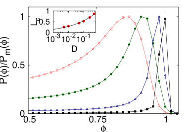
Figure 4: (Color online) Passive-advection model: (Left panel) Pseudo-gray-scale plots of the order parameter $\phi$ for different values of diffusivity $D$ (cf.Fig. 1). (Right panel) Plots of $P(\phi)/P_{m}(\phi)$, in the vicinity of the maximum at $\phi_{+}$ (cf.Fig. 2(c));the inset shows that $L_{c}\approx D^{0.27}$ (black line), which is in stark contrast to the Cahn-Hilliard-Navier-Stokes result in the inset of Fig. 2(a).

References

- (1) R. Fjørtoft, Tellus 5, 226 (1953).
- (2) R. H. Kraichnan, Phys. Fluids 10, 1417 (1967).
- (3) C. Leith, Physics of Fluids 11, 671 (1968).
- (4) G. K. Batchelor, Phys. Fluids Suppl. II 12, 233 (1969).
- (5) M. Lesieur, Turbulence in Fluids, Vol. 84 of Fluid Mechanics and Its Applications (Springer, The Netherlands, 2008).
- (6) M.E. Fisher, Rep. Prog. Phys. 30, 615 (1967).
- (7) A. Kumar, H. R. Krishnamurthy, and E. S. R. Gopal, Phys. Rep. 98, 57 (1983).
- (8) M. Kardar, Statistical Physics of Fields (Cambridge University Press, UK, 2007).
- (9) J. S. Huang, S. Vernon, and N. C. Wong, Phys. Rev. Lett. 33, 140 (1974).
- (10) J. D. Gunton, M. San Miguel, and P. S. Sahni, in Phase Transitions and Critical Phenomena, edited by C. Domb and J. Lebowitz (Academic Press, London, 1983), Vol. 8, Chap. The Dynamics of First Order Phase Transitions, p. 269.
- (11) A. Onuki, Phase Transition Dynamics (Cambridge University Press, UK, 2002).
- (12) I. M. Lifshitz and V. V. Slyozov, J. Phys. Chem. Solids 19, 35 (1959).
- (13) H. Furukawa, Phys. Rev. A 31, 1103 (1985).
- (14) E. D. Siggia, Phys. Rev. A 20, 595 (1979).
- (15) A. J. Bray, Adv. Phys. 43, 357 (1994).
- (16) A. J. Wagner and J. M. Yeomans, Phys. Rev. Lett. 80, 1429 (1998).
- (17) V. M. Kendon, Phys. Rev. E 61, R6071 (2000).
- (18) V. M. Kendon et al., J. Fluid Mech. 440, 147 (2001).
- (19) S. Puri, in Kinetics of Phase Transitions, edited by S. Puri and V. Wadhawan (CRC Press, Boca Raton, US, 2009), Vol. 6, p. 437.
- (20) M. E. Cates, arXiv:1209.2209v1, ”Lecture notes for Les Houches 2012 Summer School on Soft Interfaces”.
- (21) C. Datt, S. P. Thampi, and R. Govindarajan, Phys. Rev. E 91, 010101 (2015).
- (22) S. Berti, G. Boffetta, M. Cencini, and A. Vulpiani, Phys. Rev. Lett. 95, 224501 (2005).
- (23) P. Perlekar, R. Benzi, H.J.H. Clercx, D.R. Nelson, and F. Toschi, Phys. Rev. Lett. 112, 014502 (2014).
- (24) J. O. Hinze, A.I.Ch.E. Journal 1, 289 (1955).
- (25) P. Hohenburg and B. Halperin, Rev. Mod. Phys. 49, 435 (1977).
- (26) J. Cahn, Trans. Metall. Soc. AIME 242, 166 (1968).
- (27) P. Perlekar and R. Pandit, New Journal of Physics 11, 073003 (2009).
- (28) R. Pandit, P. Perlekar, and S. S. Ray, Pramana 73, 179 (2009).
- (29) G. Boffetta and R. E. Ecke, J. Fluid Mech. 44, 427 (2012).
- (30) C. Canuto, M. Y. Hussaini, A. Quarteroni, and T. A. Zang, Spectral methods in Fluid Dynamics (Spinger-Verlag, Berlin, 1988).
- (31) S. M. Cox and P. C. Matthews, Journal of Computational Physics 176, 430 (2002).
- (32) C. K. Chan, W. I. Goldburg, and J. V. Maher, Phys. Rev. A 35, 1756 (1987).
- (33) R. Ruiz and D. R. Nelson, Phys. Rev. A 23, 3224 (1981).
- (34) D. J. Pine, N. Easwar, J. V. Maher, and W. I. Goldburg, Phys. Rev. A 29, 308 (1984).
- (35) J. A. Aronovitz and D. R. Nelson, Phys. Rev. A 29, 2012 (1984).
- (36) T. Hashimoto, K. Matsuzaka, E. Moses, and A. Onuki, Phys. Rev. Lett. 74, 126 (1995).
- (37) A. M. Lacasta, J. M. Sancho, and F. Sagués, Phys. Rev. Lett. 75, 1791 (1995).
- (38) A. Onuki, J. Phys. Condens. Matter 9, 6119 (1997).
- (39) L. Berthier, J.-L. Barrat, and J. Kurchan, Phys. Rev. Lett. 86, 2014 (2001).
- (40) L. Ó Náraigh and J.-L. Thiffeault, Phys. Rev. E 75, 016216 (2007); L. Ó Náraigh, S. Shun, and J.-L. Thiffeault, arXiv:1407.7666 .
- (41) L. Berthier, Phys. Rev. E 63, 051503 (2001).
- (42) F. J. Muzzio, M. Tjahjadi, and J. M. Ottino, Phys. Rev. Lett. 67, 54 (1991).
- (43) M.H. Jensen and P. Olesen, Physica D 111, 243 (1998); S.S. Ray and A. Basu, Phys. Rev. E 84, 036316 (2011).
- (44) T. H. Solomon, S. Tomas, and J. L. Warner, Phys. Rev. Lett. 77, 2682 (1996); T. H. Solomon, S. Tomas, and J. L. Warner, Phys. Fluids 10, 342 (1998); T. H. Solomon, B. R. Wallace, N. S. Miller, and C. J. L. Spohn, Commun Nonlinear Sci Numer Simul 8, 239 (2003).
- (45) See Supplemental Material at [URL to be inserted by publisher] for the parameters of our simulations.