Update estimation of diffusion parameter
observed at high frequency

Yusuke Shimizu Graduate School of Mathematics, Kyushu University. 744 Motooka, Nishi-ku, Fukuoka 819-0395, Japan. y-shimizu@math.kyushu-u.ac.jp
Abstract.

We propose an update estimation method for a diffusion parameter from high-frequency dependent data under a nuisance drift element. We ensure the asymptotic equivalence of the estimator to the corresponding quasi-MLE, which has the asymptotic normality and the asymptotic efficiency. We give a simulation example to illustrate the theory.

Key words and phrases:
Diffusion process, High-frequency sampling, Recursive estimation

1. Introduction

In general, under some appropriate conditions, M𝑀M-estimators enjoy some nice properties, for example, the asymptotic efficiency of (quasi-)MLE and oracle properties of regularized estimators. However, it may suffer from heavy computation load since it is batch estimation in the sense that we have to optimize the appropriate objective function. It would be of great help to be able to carry out recursive estimation, where we update the estimator by doing some fine tuning of the previous one. In this way, it enables us to process enormous data effectively. Recursive estimation is established as an application of stochastic approximation theory, which is mainly used in control system and computer science (see e.g., Robbins and Monro [9], Nevel’son and Khas’minskii [8], Dvoretzky [2], Borkar [1]). The case of independent data was developed by, among others, Fabian [3] and [4]. We refer to Sharia [10], [11], [12] and [13] for asymptotics of time-series model recursive estimator. See Kutoyants [6, Section 2.6.6] and Lazrieva et al. [7] as well as the references therein for the case of continuous-time data from a diffusion model.

The model we consider through this paper is the scaled Wiener process with drift:

Xt=∫0tΞΌs​𝑑s+β​wt,subscript𝑋𝑑superscriptsubscript0𝑑subscriptπœ‡π‘ differential-d𝑠𝛽subscript𝑀𝑑\displaystyle X_{t}=\int_{0}^{t}\mu_{s}ds+\sqrt{\beta}w_{t}, (1)

where ΞΌπœ‡\mu is a random and time-varying nuisance process. Suppose that we observe only discrete-time sample (Xtjn)j=0nsuperscriptsubscriptsubscript𝑋subscriptsuperscript𝑑𝑛𝑗𝑗0𝑛(X_{t^{n}_{j}})_{j=0}^{n} for tjn=j​hnsubscriptsuperscript𝑑𝑛𝑗𝑗subscriptβ„Žπ‘›t^{n}_{j}=jh_{n} with hnβ†’0β†’subscriptβ„Žπ‘›0h_{n}\to 0, where Tn:=n​hnβ†’βˆžassignsubscript𝑇𝑛𝑛subscriptβ„Žπ‘›β†’T_{n}:=nh_{n}\rightarrow\infty. We know that the quasi-MLE of a true value Ξ²0subscript𝛽0\beta_{0} with regarding μ≑0πœ‡0\mu\equiv 0 is

Ξ²^nq​m​l​e=1Tnβ€‹βˆ‘j=1n(Ξ”jn​X)2,superscriptsubscript^π›½π‘›π‘žπ‘šπ‘™π‘’1subscript𝑇𝑛superscriptsubscript𝑗1𝑛superscriptsuperscriptsubscriptΔ𝑗𝑛𝑋2\displaystyle\hat{\beta}_{n}^{qmle}=\frac{1}{T_{n}}\sum_{j=1}^{n}(\Delta_{j}^{n}X)^{2}, (2)

where Ξ”jn​X=Xtjnβˆ’Xtjβˆ’1nsuperscriptsubscriptΔ𝑗𝑛𝑋subscript𝑋superscriptsubscript𝑑𝑗𝑛subscript𝑋superscriptsubscript𝑑𝑗1𝑛\Delta_{j}^{n}X=X_{t_{j}^{n}}-X_{t_{j-1}^{n}}, and Ξ²^nq​m​l​esuperscriptsubscript^π›½π‘›π‘žπ‘šπ‘™π‘’\hat{\beta}_{n}^{qmle} has the asymptotic normality and the asymptotic efficiency. The aim of this paper is to propose an update estimation method for the diffusion parameter β𝛽\beta under the nuisance drift element ∫μs​𝑑ssubscriptπœ‡π‘ differential-d𝑠\int\mu_{s}ds. Specifically, we wish to construct a sequence of estimates Ξ²^0n,Ξ²^1n,Ξ²^2n,…,Ξ²^nnsuperscriptsubscript^𝛽0𝑛superscriptsubscript^𝛽1𝑛superscriptsubscript^𝛽2𝑛…superscriptsubscript^𝛽𝑛𝑛\hat{\beta}_{0}^{n},\hat{\beta}_{1}^{n},\hat{\beta}_{2}^{n},\ldots,\hat{\beta}_{n}^{n}, computed in a recursive manner, in such a way that for any j≀n𝑗𝑛j\leq n, the difference Ξ²^jnβˆ’Ξ²^jβˆ’1nsuperscriptsubscript^𝛽𝑗𝑛superscriptsubscript^𝛽𝑗1𝑛\hat{\beta}_{j}^{n}-\hat{\beta}_{j-1}^{n} is a function described by Ξ²^jβˆ’1nsuperscriptsubscript^𝛽𝑗1𝑛\hat{\beta}_{j-1}^{n}, hnsubscriptβ„Žπ‘›h_{n}, j𝑗j, and some (not all) data, and Ξ²^nnsuperscriptsubscript^𝛽𝑛𝑛\hat{\beta}_{n}^{n} exhibits suitable convergence property for an arbitrary initial value Ξ²^00superscriptsubscript^𝛽00\hat{\beta}_{0}^{0}. Usually this estimator does not require any numerically hard optimization, while its asymptotic behavior does require careful investigation. Note the difference from the recursive (online) estimation for sample X1,X2,…subscript𝑋1subscript𝑋2…X_{1},X_{2},\dots, where each successive estimator is obtained by using data observed one after another. We will bring about good asymptotic property of Ξ²^nnsuperscriptsubscript^𝛽𝑛𝑛\hat{\beta}_{n}^{n} as efficient as the quasi-MLE, i.e we ensure the asymptotic equivalence of Ξ²^nnsuperscriptsubscript^𝛽𝑛𝑛\hat{\beta}_{n}^{n} to Ξ²^nq​m​l​esuperscriptsubscript^π›½π‘›π‘žπ‘šπ‘™π‘’\hat{\beta}_{n}^{qmle}:

n​(Ξ²^nq​m​l​eβˆ’Ξ²^nn)→𝑃0.𝑃→𝑛superscriptsubscript^π›½π‘›π‘žπ‘šπ‘™π‘’superscriptsubscript^𝛽𝑛𝑛0\displaystyle\sqrt{n}(\hat{\beta}_{n}^{qmle}-\hat{\beta}_{n}^{n})\xrightarrow{P}0.

This paper is organized as follows. In Section 2, we propose an update formula and give a main theorem with the proof. We consider an example and present the simulation result to illustrate the theory in Section 3.

2. Main result

We consider the scaled Wiener process with drift (1), where ΞΌπœ‡\mu is a random and time-varying nuisance process and Ξ²βˆˆΞ˜Ξ²βŠ‚β„+𝛽subscriptΞ˜π›½subscriptℝ\beta\in\Theta_{\beta}\subset\mathbb{R}_{+}. We denote by (PΞ²:β∈Θβ):subscript𝑃𝛽𝛽subscriptΞ˜π›½(P_{\beta}:\beta\in\Theta_{\beta}) the family of distributions of X𝑋X associated with β𝛽\beta: Pβ​(B):=P∘Xβˆ’1​(B)assignsubscript𝑃𝛽𝐡𝑃superscript𝑋1𝐡P_{\beta}(B):=P\circ X^{-1}(B), Bβˆˆβ„¬β€‹(π’žβ€‹(ℝ+;ℝ))π΅β„¬π’žsubscriptℝℝB\in\mathcal{B}\big{(}\mathcal{C}(\mathbb{R}_{+};\mathbb{R})\big{)}. Let β„±t:=σ​{X0,(ws)s≀t}assignsubscriptβ„±π‘‘πœŽsubscript𝑋0subscriptsubscript𝑀𝑠𝑠𝑑\mathcal{F}_{t}:=\sigma\{X_{0},(w_{s})_{s\leq t}\}, the underlying filtration. Suppose that we observe only discrete-time sample 𝐗n:=(Xtjn)j=0nassignsubscript𝐗𝑛superscriptsubscriptsubscript𝑋superscriptsubscript𝑑𝑗𝑛𝑗0𝑛\mathbf{X}_{n}:=(X_{t_{j}^{n}})_{j=0}^{n} for tjn=j​hnsuperscriptsubscript𝑑𝑗𝑛𝑗subscriptβ„Žπ‘›t_{j}^{n}=jh_{n} with hnβ†’0β†’subscriptβ„Žπ‘›0h_{n}\to 0, where Tn=n​hnβ†’βˆžsubscript𝑇𝑛𝑛subscriptβ„Žπ‘›β†’T_{n}=nh_{n}\to\infty. We wish to estimate the true value Ξ²0∈Θβsubscript𝛽0subscriptΞ˜π›½\beta_{0}\in\Theta_{\beta} based on 𝐗nsubscript𝐗𝑛\mathbf{X}_{n}. As is well known, the quasi-likelihood function, denote by 𝕄nsubscript𝕄𝑛\mathbb{M}_{n}, with regarding μ≑0πœ‡0\mu\equiv 0 is

𝕄n​(Ξ²)=βˆ‘j=1nlog⁑12​π​β​hn​exp​(βˆ’(Ξ”jn​X)22​β​hn).subscript𝕄𝑛𝛽superscriptsubscript𝑗1𝑛12πœ‹π›½subscriptβ„Žπ‘›expsuperscriptsuperscriptsubscriptΔ𝑗𝑛𝑋22𝛽subscriptβ„Žπ‘›\displaystyle\mathbb{M}_{n}(\beta)=\sum_{j=1}^{n}\log\frac{1}{\sqrt{2\pi\beta h_{n}}}{\rm exp}\left(-\frac{(\Delta_{j}^{n}X)^{2}}{2\beta h_{n}}\right). (3)

Therefore, the quasi-MLE of β𝛽\beta is (2), and Ξ²^nq​m​l​esuperscriptsubscript^π›½π‘›π‘žπ‘šπ‘™π‘’\hat{\beta}_{n}^{qmle} has the asymptotic normality

n​(Ξ²^nq​m​l​eβˆ’Ξ²0)β†’β„’N​(0,2​β02)ℒ→𝑛superscriptsubscript^π›½π‘›π‘žπ‘šπ‘™π‘’subscript𝛽0𝑁02superscriptsubscript𝛽02\displaystyle\sqrt{n}(\hat{\beta}_{n}^{qmle}-\beta_{0})\xrightarrow{\mathcal{L}}N(0,2\beta_{0}^{2})

and the asymptotic efficiency. The aim of this paper is to propose an update estimation method for the diffusion parameter β𝛽\beta having the form

Ξ²^jn=Ξ²^jβˆ’1n+Fn,j​(Ξ²^jβˆ’1n;Xtjn),j≀n,formulae-sequencesuperscriptsubscript^𝛽𝑗𝑛superscriptsubscript^𝛽𝑗1𝑛subscript𝐹𝑛𝑗superscriptsubscript^𝛽𝑗1𝑛subscript𝑋superscriptsubscript𝑑𝑗𝑛𝑗𝑛\displaystyle\hat{\beta}_{j}^{n}=\hat{\beta}_{j-1}^{n}+F_{n,j}(\hat{\beta}_{j-1}^{n};X_{t_{j}^{n}}),\qquad j\leq n,

where Fn,jsubscript𝐹𝑛𝑗F_{n,j} is an appropriate fine tuning function. The upper index n𝑛n implies that we have the data set 𝐗nsubscript𝐗𝑛\mathbf{X}_{n}. Under the nuisance drift element ∫μs​𝑑ssubscriptπœ‡π‘ differential-d𝑠\int\mu_{s}ds, we ensure the asymptotic equivalence of Ξ²^nnsuperscriptsubscript^𝛽𝑛𝑛\hat{\beta}_{n}^{n} to Ξ²^nq​m​l​esuperscriptsubscript^π›½π‘›π‘žπ‘šπ‘™π‘’\hat{\beta}_{n}^{qmle}. Therefore, the asymptotic normality and the asymptotic efficiency of Ξ²^nnsuperscriptsubscript^𝛽𝑛𝑛\hat{\beta}_{n}^{n} hold.

We now define some notations: denote ansubscriptπ‘Žπ‘›a_{n} and V​(Ξ²0)𝑉subscript𝛽0V(\beta_{0}) by the convergence rate and the asymptotic variance of Ξ²^nq​m​l​esuperscriptsubscript^π›½π‘›π‘žπ‘šπ‘™π‘’\hat{\beta}_{n}^{qmle}, respectively, i.e., an=nsubscriptπ‘Žπ‘›π‘›a_{n}=\sqrt{n} and V​(Ξ²0)=2​β02𝑉subscript𝛽02superscriptsubscript𝛽02V(\beta_{0})=2\beta_{0}^{2}. We also define the quasi-likelihood function (3) as 𝕄n(Ξ²)=:βˆ‘j=1nmn,j(Ξ²)\mathbb{M}_{n}(\beta)=:\sum_{j=1}^{n}m_{n,j}(\beta). Then, we propose the following update formula:

Ξ²^jnsuperscriptsubscript^𝛽𝑗𝑛\displaystyle\hat{\beta}_{j}^{n} =Ξ²^jβˆ’1n+V​(Ξ²^jβˆ’1n)aj2β€‹βˆ‚mn,j​(Ξ²^jβˆ’1n),j≀n.formulae-sequenceabsentsuperscriptsubscript^𝛽𝑗1𝑛𝑉superscriptsubscript^𝛽𝑗1𝑛superscriptsubscriptπ‘Žπ‘—2subscriptπ‘šπ‘›π‘—superscriptsubscript^𝛽𝑗1𝑛𝑗𝑛\displaystyle=\hat{\beta}_{j-1}^{n}+\frac{V(\hat{\beta}_{j-1}^{n})}{a_{j}^{2}}\partial m_{n,j}(\hat{\beta}_{j-1}^{n}),\qquad j\leq n. (4)

Note that, in finite sample, this formula is more stable than the one which is derived by direct using of the Newton-Raphson method. We have

V​(Ξ²)aj2=2​β2j,βˆ‚mn,j​(Ξ²)=βˆ’12​β+(Ξ”jn​X)22​hn​β2,j≀n,formulae-sequence𝑉𝛽superscriptsubscriptπ‘Žπ‘—22superscript𝛽2𝑗formulae-sequencesubscriptπ‘šπ‘›π‘—π›½12𝛽superscriptsuperscriptsubscriptΔ𝑗𝑛𝑋22subscriptβ„Žπ‘›superscript𝛽2𝑗𝑛\displaystyle\frac{V(\beta)}{a_{j}^{2}}=\frac{2\beta^{2}}{j},\qquad\partial m_{n,j}(\beta)=-\frac{1}{2\beta}+\frac{(\Delta_{j}^{n}X)^{2}}{2h_{n}\beta^{2}},\qquad j\leq n,

hence the update formula (4) is

Ξ²^jnsuperscriptsubscript^𝛽𝑗𝑛\displaystyle\hat{\beta}_{j}^{n} =Ξ²^jβˆ’1n+2​(Ξ²^jβˆ’1n)2j​{βˆ’12​β^jβˆ’1n+(Ξ”jn​X)22​hn​(Ξ²^jβˆ’1n)2}absentsuperscriptsubscript^𝛽𝑗1𝑛2superscriptsuperscriptsubscript^𝛽𝑗1𝑛2𝑗12superscriptsubscript^𝛽𝑗1𝑛superscriptsuperscriptsubscriptΔ𝑗𝑛𝑋22subscriptβ„Žπ‘›superscriptsuperscriptsubscript^𝛽𝑗1𝑛2\displaystyle=\hat{\beta}_{j-1}^{n}+\frac{2(\hat{\beta}_{j-1}^{n})^{2}}{j}\left\{-\frac{1}{2\hat{\beta}_{j-1}^{n}}+\frac{(\Delta_{j}^{n}X)^{2}}{2h_{n}(\hat{\beta}_{j-1}^{n})^{2}}\right\}
=(1βˆ’1j)​β^jβˆ’1n+(Ξ”jn​X)2j​hn,j≀n.formulae-sequenceabsent11𝑗superscriptsubscript^𝛽𝑗1𝑛superscriptsuperscriptsubscriptΔ𝑗𝑛𝑋2𝑗subscriptβ„Žπ‘›π‘—π‘›\displaystyle=\Big{(}1-\frac{1}{j}\Big{)}\hat{\beta}_{j-1}^{n}+\frac{(\Delta_{j}^{n}X)^{2}}{jh_{n}},\qquad j\leq n. (5)

Note that right-hand side of (5) is positive a.s. for any initial value Ξ²^0n∈Θβsuperscriptsubscript^𝛽0𝑛subscriptΞ˜π›½\hat{\beta}_{0}^{n}\in\Theta_{\beta}. Then, for any nβˆˆβ„•π‘›β„•n\in\mathbb{N} and j≀n𝑗𝑛j\leq n we define

ΞΌΒ―n,j:=1hnβ€‹βˆ«tjβˆ’1tjΞΌs​𝑑s,Yn,j:=Ξ”jn​Xβˆ’hn​μ¯n,jhn​β0.formulae-sequenceassignsubscriptΒ―πœ‡π‘›π‘—1subscriptβ„Žπ‘›superscriptsubscriptsubscript𝑑𝑗1subscript𝑑𝑗subscriptπœ‡π‘ differential-d𝑠assignsubscriptπ‘Œπ‘›π‘—superscriptsubscriptΔ𝑗𝑛𝑋subscriptβ„Žπ‘›subscriptΒ―πœ‡π‘›π‘—subscriptβ„Žπ‘›subscript𝛽0\displaystyle\overline{\mu}_{n,j}:=\frac{1}{h_{n}}\int_{t_{j-1}}^{t_{j}}\mu_{s}ds,\qquad Y_{n,j}:=\frac{\Delta_{j}^{n}X-h_{n}\overline{\mu}_{n,j}}{\sqrt{h_{n}\beta_{0}}}.

Note that Yn,j∼i.i.d.N​(0,1)Y_{n,j}\stackrel{{\scriptstyle i.i.d.}}{{\sim}}N(0,1) for j≀n𝑗𝑛j\leq n. Now, we set two assumptions:

Assumption 2.1.

There exists 0<Ο΅0<1/20subscriptitalic-Ο΅0120<\epsilon_{0}<1/2 such that Tn≲nΟ΅0less-than-or-similar-tosubscript𝑇𝑛superscript𝑛subscriptitalic-Ο΅0T_{n}\lesssim n^{\epsilon_{0}}.

Assumption 2.2.
hnnβ€‹βˆ‘j=1nEΞ²0​[Yn,j​μ¯n,j|β„±tjβˆ’1n]→𝑃0;𝑃→subscriptβ„Žπ‘›π‘›superscriptsubscript𝑗1𝑛subscript𝐸subscript𝛽0delimited-[]conditionalsubscriptπ‘Œπ‘›π‘—subscriptΒ―πœ‡π‘›π‘—subscriptβ„±superscriptsubscript𝑑𝑗1𝑛0\displaystyle\sqrt{\frac{h_{n}}{n}}\sum_{j=1}^{n}E_{\beta_{0}}\left[Y_{n,j}\overline{\mu}_{n,j}\big{|}\mathcal{F}_{t_{j-1}^{n}}\right]\xrightarrow{P}0; (6)
supn>0supt≀TnEΞ²0​[|ΞΌt|2]<∞.subscriptsupremum𝑛0subscriptsupremum𝑑subscript𝑇𝑛subscript𝐸subscript𝛽0delimited-[]superscriptsubscriptπœ‡π‘‘2\displaystyle\sup_{n>0}\sup_{t\leq T_{n}}E_{\beta_{0}}\left[|\mu_{t}|^{2}\right]<\infty. (7)

The notation An≲Bnless-than-or-similar-tosubscript𝐴𝑛subscript𝐡𝑛A_{n}\lesssim B_{n} in Assumption 2.1 means that supn(An/Bn)<∞subscriptsupremum𝑛subscript𝐴𝑛subscript𝐡𝑛\sup_{n}(A_{n}/B_{n})<\infty. The following Theorem 2.3 is a main result in this paper.

Theorem 2.3.

Consider the model (1). Assume that Assumptions 2.1 and 2.2 hold. Then, for any Ξ²^0n∈Θβsuperscriptsubscript^𝛽0𝑛subscriptΞ˜π›½\hat{\beta}_{0}^{n}\in\Theta_{\beta} the update formula (5) generates an estimator Ξ²^nnsuperscriptsubscript^𝛽𝑛𝑛\hat{\beta}_{n}^{n}, which is asymptotic equivalent to Ξ²^nq​m​l​esuperscriptsubscript^π›½π‘›π‘žπ‘šπ‘™π‘’\hat{\beta}_{n}^{qmle}:

n​(Ξ²^nq​m​l​eβˆ’Ξ²^nn)→𝑃0.𝑃→𝑛superscriptsubscript^π›½π‘›π‘žπ‘šπ‘™π‘’superscriptsubscript^𝛽𝑛𝑛0\displaystyle\sqrt{n}(\hat{\beta}_{n}^{qmle}-\hat{\beta}_{n}^{n})\xrightarrow{P}0. (8)

Therefore, it has the asymptotic normality:

n​(Ξ²^nnβˆ’Ξ²0)β†’β„’N​(0,2​β02)ℒ→𝑛superscriptsubscript^𝛽𝑛𝑛subscript𝛽0𝑁02superscriptsubscript𝛽02\displaystyle\sqrt{n}(\hat{\beta}_{n}^{n}-\beta_{0})\xrightarrow{\mathcal{L}}N(0,2\beta_{0}^{2})

and the asymptotic efficiency.

Proof.

To prove the theorem, we use the result of Sharia [13, Lemma 1]. We change some notations from the original ones of Sharia [13] in terms of a triangular array of random variables. We drop the index n𝑛n to simplify some notations. We can rewrite (5) to

Ξ²^jsubscript^𝛽𝑗\displaystyle\hat{\beta}_{j} =Ξ²^jβˆ’1+2​β^jβˆ’12j​{βˆ’12​β^jβˆ’1+(hn​β0​Yj+hn​μ¯j)22​hn​β^jβˆ’12}absentsubscript^𝛽𝑗12superscriptsubscript^𝛽𝑗12𝑗12subscript^𝛽𝑗1superscriptsubscriptβ„Žπ‘›subscript𝛽0subscriptπ‘Œπ‘—subscriptβ„Žπ‘›subscriptΒ―πœ‡π‘—22subscriptβ„Žπ‘›superscriptsubscript^𝛽𝑗12\displaystyle=\hat{\beta}_{j-1}+\frac{2\hat{\beta}_{j-1}^{2}}{j}\left\{-\frac{1}{2\hat{\beta}_{j-1}}+\frac{(\sqrt{h_{n}\beta_{0}}Y_{j}+h_{n}\overline{\mu}_{j})^{2}}{2h_{n}\hat{\beta}_{j-1}^{2}}\right\}
=Ξ²^jβˆ’1+2​β^jβˆ’12j​{βˆ’12​β^jβˆ’1+Ξ²02​β^jβˆ’12​(Yj+ΞΌΒ―j​hnΞ²0)2}absentsubscript^𝛽𝑗12superscriptsubscript^𝛽𝑗12𝑗12subscript^𝛽𝑗1subscript𝛽02superscriptsubscript^𝛽𝑗12superscriptsubscriptπ‘Œπ‘—subscriptΒ―πœ‡π‘—subscriptβ„Žπ‘›subscript𝛽02\displaystyle=\hat{\beta}_{j-1}+\frac{2\hat{\beta}_{j-1}^{2}}{j}\left\{-\frac{1}{2\hat{\beta}_{j-1}}+\frac{\beta_{0}}{2\hat{\beta}_{j-1}^{2}}\left(Y_{j}+\overline{\mu}_{j}\sqrt{\frac{h_{n}}{\beta_{0}}}\right)^{2}\right\}
=:Ξ²^jβˆ’1+Ξ“j(Ξ²^jβˆ’1)βˆ’1β‹…Οˆn,j(Ξ²^jβˆ’1),\displaystyle=:\hat{\beta}_{j-1}+\Gamma_{j}(\hat{\beta}_{j-1})^{-1}\cdot\psi_{n,j}(\hat{\beta}_{j-1}),

where

Ξ“j​(Ξ²):=j2​β2,ψn,j​(Ξ²):=βˆ’12​β+Ξ²02​β2​(Yj+ΞΌΒ―j​hnΞ²0)2.formulae-sequenceassignsubscriptΓ𝑗𝛽𝑗2superscript𝛽2assignsubscriptπœ“π‘›π‘—π›½12𝛽subscript𝛽02superscript𝛽2superscriptsubscriptπ‘Œπ‘—subscriptΒ―πœ‡π‘—subscriptβ„Žπ‘›subscript𝛽02\displaystyle\Gamma_{j}(\beta):=\frac{j}{2\beta^{2}},\qquad\psi_{n,j}(\beta):=-\frac{1}{2\beta}+\frac{\beta_{0}}{2\beta^{2}}\left(Y_{j}+\overline{\mu}_{j}\sqrt{\frac{h_{n}}{\beta_{0}}}\right)^{2}.

Moreover, we define the following notations:

bn,j​(Ξ²0,djβˆ’1)=EΞ²0​[ψn,j​(Ξ²^jβˆ’1)|β„±tjβˆ’1];subscript𝑏𝑛𝑗subscript𝛽0subscript𝑑𝑗1subscript𝐸subscript𝛽0delimited-[]conditionalsubscriptπœ“π‘›π‘—subscript^𝛽𝑗1subscriptβ„±subscript𝑑𝑗1\displaystyle b_{n,j}(\beta_{0},d_{j-1})=E_{\beta_{0}}\left[\psi_{n,j}(\hat{\beta}_{j-1})\big{|}\mathcal{F}_{t_{j-1}}\right];
Rn,j​(Ξ²0,djβˆ’1)=Ξ“j​(Ξ²0)​Γjβˆ’1​(Ξ²^jβˆ’1)​bn,j​(Ξ²0,djβˆ’1);subscript𝑅𝑛𝑗subscript𝛽0subscript𝑑𝑗1subscriptΓ𝑗subscript𝛽0superscriptsubscriptΓ𝑗1subscript^𝛽𝑗1subscript𝑏𝑛𝑗subscript𝛽0subscript𝑑𝑗1\displaystyle R_{n,j}(\beta_{0},d_{j-1})=\Gamma_{j}(\beta_{0})\Gamma_{j}^{-1}(\hat{\beta}_{j-1})b_{n,j}(\beta_{0},d_{j-1});
β„°n,j​(Ξ²0,djβˆ’1)=Ξ“j​(Ξ²0)​Γjβˆ’1​(Ξ²^jβˆ’1)​{ψn,j​(Ξ²^jβˆ’1)βˆ’bn,j​(Ξ²0,djβˆ’1)}βˆ’Οˆn,j​(Ξ²0),subscriptℰ𝑛𝑗subscript𝛽0subscript𝑑𝑗1subscriptΓ𝑗subscript𝛽0superscriptsubscriptΓ𝑗1subscript^𝛽𝑗1subscriptπœ“π‘›π‘—subscript^𝛽𝑗1subscript𝑏𝑛𝑗subscript𝛽0subscript𝑑𝑗1subscriptπœ“π‘›π‘—subscript𝛽0\displaystyle\mathcal{E}_{n,j}(\beta_{0},d_{j-1})=\Gamma_{j}(\beta_{0})\Gamma_{j}^{-1}(\hat{\beta}_{j-1})\{\psi_{n,j}(\hat{\beta}_{j-1})-b_{n,j}(\beta_{0},d_{j-1})\}-\psi_{n,j}(\beta_{0}),

where dj:=Ξ²^jβˆ’Ξ²0assignsubscript𝑑𝑗subscript^𝛽𝑗subscript𝛽0d_{j}:=\hat{\beta}_{j}-\beta_{0} and j≀n𝑗𝑛j\leq n, and introduce the conditions of Sharia [13, Lemma 1] applied to our model setting:

  1. (i)
    (n)2Ξ“n​(Ξ²0)→ℒη​(Ξ²0)β„’β†’superscript𝑛2subscriptΓ𝑛subscript𝛽0πœ‚subscript𝛽0\displaystyle\frac{(\sqrt{n})^{2}}{\Gamma_{n}(\beta_{0})}\xrightarrow{\mathcal{L}}\eta(\beta_{0})

    w.r.t. PΞ²0subscript𝑃subscript𝛽0P_{\beta_{0}}, where η​(Ξ²0)πœ‚subscript𝛽0\eta(\beta_{0}) is a random variable with η​(Ξ²0)<βˆžβ€‹PΞ²0βˆ’a.s.formulae-sequenceπœ‚subscript𝛽0subscript𝑃subscript𝛽0as\eta(\beta_{0})<\infty\ P_{\beta_{0}}{\rm\mathchar 45\relax a.s.};

  2. (ii)
    limnβ†’βˆž1nβ€‹βˆ‘j=1n{(Ξ“j​(Ξ²0)βˆ’Ξ“jβˆ’1​(Ξ²0))​djβˆ’1+Rn,j​(Ξ²0,djβˆ’1)}=0subscript→𝑛1𝑛superscriptsubscript𝑗1𝑛subscriptΓ𝑗subscript𝛽0subscriptΓ𝑗1subscript𝛽0subscript𝑑𝑗1subscript𝑅𝑛𝑗subscript𝛽0subscript𝑑𝑗10\displaystyle\lim_{n\rightarrow\infty}\frac{1}{\sqrt{n}}\sum_{j=1}^{n}\big{\{}\big{(}\Gamma_{j}(\beta_{0})-\Gamma_{j-1}(\beta_{0})\big{)}d_{j-1}+R_{n,j}(\beta_{0},d_{j-1})\big{\}}=0

    in probability PΞ²0subscript𝑃subscript𝛽0P_{\beta_{0}};

  3. (iii)
    limnβ†’βˆž1nβ€‹βˆ‘j=1nβ„°n,j​(Ξ²0,djβˆ’1)=0subscript→𝑛1𝑛superscriptsubscript𝑗1𝑛subscriptℰ𝑛𝑗subscript𝛽0subscript𝑑𝑗10\displaystyle\lim_{n\rightarrow\infty}\frac{1}{\sqrt{n}}\sum_{j=1}^{n}\mathcal{E}_{n,j}(\beta_{0},d_{j-1})=0

    in probability PΞ²0subscript𝑃subscript𝛽0P_{\beta_{0}}.


Now, let us show the above conditions and derive the local asymptotic linearity of Ξ²^nnsuperscriptsubscript^𝛽𝑛𝑛\hat{\beta}_{n}^{n}:

n​(Ξ²^nnβˆ’Ξ²^nβˆ—)→𝑃0,𝑃→𝑛superscriptsubscript^𝛽𝑛𝑛superscriptsubscript^π›½π‘›βˆ—0\displaystyle\sqrt{n}(\hat{\beta}_{n}^{n}-\hat{\beta}_{n}^{\ast})\xrightarrow{P}0, (9)

where

Ξ²^nβˆ—=Ξ²0+Ξ“nβˆ’1​(Ξ²0)β€‹βˆ‘j=1nψn,j​(Ξ²0)superscriptsubscript^π›½π‘›βˆ—subscript𝛽0superscriptsubscriptΓ𝑛1subscript𝛽0superscriptsubscript𝑗1𝑛subscriptπœ“π‘›π‘—subscript𝛽0\displaystyle\hat{\beta}_{n}^{\ast}=\beta_{0}+\Gamma_{n}^{-1}(\beta_{0})\sum_{j=1}^{n}\psi_{n,j}(\beta_{0})

is a linear statistic. Clearly, (i) holds since we have n/Ξ“n​(Ξ²0)=2​β02𝑛subscriptΓ𝑛subscript𝛽02superscriptsubscript𝛽02n/\Gamma_{n}(\beta_{0})=2\beta_{0}^{2}. To check (ii), we calculate

bn,j​(Ξ²0,djβˆ’1)subscript𝑏𝑛𝑗subscript𝛽0subscript𝑑𝑗1\displaystyle b_{n,j}(\beta_{0},d_{j-1}) =βˆ’12​β^jβˆ’1+Ξ²02​β^jβˆ’12​EΞ²0​[(Yj+ΞΌΒ―j​hnΞ²0)2|β„±tjβˆ’1]absent12subscript^𝛽𝑗1subscript𝛽02superscriptsubscript^𝛽𝑗12subscript𝐸subscript𝛽0delimited-[]conditionalsuperscriptsubscriptπ‘Œπ‘—subscriptΒ―πœ‡π‘—subscriptβ„Žπ‘›subscript𝛽02subscriptβ„±subscript𝑑𝑗1\displaystyle=-\frac{1}{2\hat{\beta}_{j-1}}+\frac{\beta_{0}}{2\hat{\beta}_{j-1}^{2}}E_{\beta_{0}}\left[\left(Y_{j}+\overline{\mu}_{j}\sqrt{\frac{h_{n}}{\beta_{0}}}\right)^{2}\Big{|}\mathcal{F}_{t_{j-1}}\right]
=βˆ’12​β^jβˆ’1+Ξ²02​β^jβˆ’12​(1+2​hnΞ²0​EΞ²0​[Yj​μ¯j|β„±tjβˆ’1]+hnΞ²0​EΞ²0​[|ΞΌΒ―j|2|β„±tjβˆ’1])absent12subscript^𝛽𝑗1subscript𝛽02superscriptsubscript^𝛽𝑗1212subscriptβ„Žπ‘›subscript𝛽0subscript𝐸subscript𝛽0delimited-[]conditionalsubscriptπ‘Œπ‘—subscriptΒ―πœ‡π‘—subscriptβ„±subscript𝑑𝑗1subscriptβ„Žπ‘›subscript𝛽0subscript𝐸subscript𝛽0delimited-[]conditionalsuperscriptsubscriptΒ―πœ‡π‘—2subscriptβ„±subscript𝑑𝑗1\displaystyle=-\frac{1}{2\hat{\beta}_{j-1}}+\frac{\beta_{0}}{2\hat{\beta}_{j-1}^{2}}\left(1+2\sqrt{\frac{h_{n}}{\beta_{0}}}E_{\beta_{0}}\left[Y_{j}\overline{\mu}_{j}\big{|}\mathcal{F}_{t_{j-1}}\right]+\frac{h_{n}}{\beta_{0}}E_{\beta_{0}}\left[|\overline{\mu}_{j}|^{2}\big{|}\mathcal{F}_{t_{j-1}}\right]\right)
=βˆ’djβˆ’12​β^jβˆ’12+hn​β0Ξ²^jβˆ’12​EΞ²0​[Yj​μ¯j|β„±tjβˆ’1]+hn2​β^jβˆ’12​EΞ²0​[|ΞΌΒ―j|2|β„±tjβˆ’1],absentsubscript𝑑𝑗12superscriptsubscript^𝛽𝑗12subscriptβ„Žπ‘›subscript𝛽0superscriptsubscript^𝛽𝑗12subscript𝐸subscript𝛽0delimited-[]conditionalsubscriptπ‘Œπ‘—subscriptΒ―πœ‡π‘—subscriptβ„±subscript𝑑𝑗1subscriptβ„Žπ‘›2superscriptsubscript^𝛽𝑗12subscript𝐸subscript𝛽0delimited-[]conditionalsuperscriptsubscriptΒ―πœ‡π‘—2subscriptβ„±subscript𝑑𝑗1\displaystyle=-\frac{d_{j-1}}{2\hat{\beta}_{j-1}^{2}}+\frac{\sqrt{h_{n}\beta_{0}}}{\hat{\beta}_{j-1}^{2}}E_{\beta_{0}}\left[Y_{j}\overline{\mu}_{j}\big{|}\mathcal{F}_{t_{j-1}}\right]+\frac{h_{n}}{2\hat{\beta}_{j-1}^{2}}E_{\beta_{0}}\left[|\overline{\mu}_{j}|^{2}\big{|}\mathcal{F}_{t_{j-1}}\right],
Rn,j​(Ξ²0,djβˆ’1)subscript𝑅𝑛𝑗subscript𝛽0subscript𝑑𝑗1\displaystyle R_{n,j}(\beta_{0},d_{j-1}) =j2​β02​2​β^jβˆ’12j​{βˆ’djβˆ’12​β^jβˆ’12+hn​β0Ξ²^jβˆ’12​EΞ²0​[Yj​μ¯j|β„±tjβˆ’1]+hn2​β^jβˆ’12​EΞ²0​[|ΞΌΒ―j|2|β„±tjβˆ’1]}absent𝑗2superscriptsubscript𝛽022superscriptsubscript^𝛽𝑗12𝑗subscript𝑑𝑗12superscriptsubscript^𝛽𝑗12subscriptβ„Žπ‘›subscript𝛽0superscriptsubscript^𝛽𝑗12subscript𝐸subscript𝛽0delimited-[]conditionalsubscriptπ‘Œπ‘—subscriptΒ―πœ‡π‘—subscriptβ„±subscript𝑑𝑗1subscriptβ„Žπ‘›2superscriptsubscript^𝛽𝑗12subscript𝐸subscript𝛽0delimited-[]conditionalsuperscriptsubscriptΒ―πœ‡π‘—2subscriptβ„±subscript𝑑𝑗1\displaystyle=\frac{j}{2\beta_{0}^{2}}\frac{2\hat{\beta}_{j-1}^{2}}{j}\left\{-\frac{d_{j-1}}{2\hat{\beta}_{j-1}^{2}}+\frac{\sqrt{h_{n}\beta_{0}}}{\hat{\beta}_{j-1}^{2}}E_{\beta_{0}}\left[Y_{j}\overline{\mu}_{j}\big{|}\mathcal{F}_{t_{j-1}}\right]+\frac{h_{n}}{2\hat{\beta}_{j-1}^{2}}E_{\beta_{0}}\left[|\overline{\mu}_{j}|^{2}\big{|}\mathcal{F}_{t_{j-1}}\right]\right\}
=1Ξ²02​(βˆ’djβˆ’12+hn​β0​EΞ²0​[Yj​μ¯j|β„±tjβˆ’1]+hn2​EΞ²0​[|ΞΌΒ―j|2|β„±tjβˆ’1]).absent1superscriptsubscript𝛽02subscript𝑑𝑗12subscriptβ„Žπ‘›subscript𝛽0subscript𝐸subscript𝛽0delimited-[]conditionalsubscriptπ‘Œπ‘—subscriptΒ―πœ‡π‘—subscriptβ„±subscript𝑑𝑗1subscriptβ„Žπ‘›2subscript𝐸subscript𝛽0delimited-[]conditionalsuperscriptsubscriptΒ―πœ‡π‘—2subscriptβ„±subscript𝑑𝑗1\displaystyle=\frac{1}{\beta_{0}^{2}}\left(-\frac{d_{j-1}}{2}+\sqrt{h_{n}\beta_{0}}E_{\beta_{0}}\left[Y_{j}\overline{\mu}_{j}\big{|}\mathcal{F}_{t_{j-1}}\right]+\frac{h_{n}}{2}E_{\beta_{0}}\left[|\overline{\mu}_{j}|^{2}\big{|}\mathcal{F}_{t_{j-1}}\right]\right).

Hence, we have

(Ξ“j​(Ξ²0)βˆ’Ξ“jβˆ’1​(Ξ²0))​djβˆ’1+Rn,j​(Ξ²0,djβˆ’1)subscriptΓ𝑗subscript𝛽0subscriptΓ𝑗1subscript𝛽0subscript𝑑𝑗1subscript𝑅𝑛𝑗subscript𝛽0subscript𝑑𝑗1\displaystyle\big{(}\Gamma_{j}(\beta_{0})-\Gamma_{j-1}(\beta_{0})\big{)}d_{j-1}+R_{n,j}(\beta_{0},d_{j-1})
=(j2​β02βˆ’jβˆ’12​β02)​djβˆ’1+1Ξ²02​(βˆ’djβˆ’12+hn​β0​EΞ²0​[Yj​μ¯j|β„±tjβˆ’1]+hn2​EΞ²0​[|ΞΌΒ―j|2|β„±tjβˆ’1])absent𝑗2superscriptsubscript𝛽02𝑗12superscriptsubscript𝛽02subscript𝑑𝑗11superscriptsubscript𝛽02subscript𝑑𝑗12subscriptβ„Žπ‘›subscript𝛽0subscript𝐸subscript𝛽0delimited-[]conditionalsubscriptπ‘Œπ‘—subscriptΒ―πœ‡π‘—subscriptβ„±subscript𝑑𝑗1subscriptβ„Žπ‘›2subscript𝐸subscript𝛽0delimited-[]conditionalsuperscriptsubscriptΒ―πœ‡π‘—2subscriptβ„±subscript𝑑𝑗1\displaystyle=\left(\frac{j}{2\beta_{0}^{2}}-\frac{j-1}{2\beta_{0}^{2}}\right)d_{j-1}+\frac{1}{\beta_{0}^{2}}\left(-\frac{d_{j-1}}{2}+\sqrt{h_{n}\beta_{0}}E_{\beta_{0}}\left[Y_{j}\overline{\mu}_{j}\big{|}\mathcal{F}_{t_{j-1}}\right]+\frac{h_{n}}{2}E_{\beta_{0}}\left[|\overline{\mu}_{j}|^{2}\big{|}\mathcal{F}_{t_{j-1}}\right]\right)
=1Ξ²02​(hn​β0​EΞ²0​[Yj​μ¯j|β„±tjβˆ’1]+hn2​EΞ²0​[|ΞΌΒ―j|2|β„±tjβˆ’1]),absent1superscriptsubscript𝛽02subscriptβ„Žπ‘›subscript𝛽0subscript𝐸subscript𝛽0delimited-[]conditionalsubscriptπ‘Œπ‘—subscriptΒ―πœ‡π‘—subscriptβ„±subscript𝑑𝑗1subscriptβ„Žπ‘›2subscript𝐸subscript𝛽0delimited-[]conditionalsuperscriptsubscriptΒ―πœ‡π‘—2subscriptβ„±subscript𝑑𝑗1\displaystyle=\frac{1}{\beta_{0}^{2}}\left(\sqrt{h_{n}\beta_{0}}E_{\beta_{0}}\left[Y_{j}\overline{\mu}_{j}\big{|}\mathcal{F}_{t_{j-1}}\right]+\frac{h_{n}}{2}E_{\beta_{0}}\left[|\overline{\mu}_{j}|^{2}\big{|}\mathcal{F}_{t_{j-1}}\right]\right),

and therefore

1nβ€‹βˆ‘j=1n{(Ξ“j​(Ξ²0)βˆ’Ξ“jβˆ’1​(Ξ²0))​djβˆ’1+Rn,j​(Ξ²0,djβˆ’1)}1𝑛superscriptsubscript𝑗1𝑛subscriptΓ𝑗subscript𝛽0subscriptΓ𝑗1subscript𝛽0subscript𝑑𝑗1subscript𝑅𝑛𝑗subscript𝛽0subscript𝑑𝑗1\displaystyle\frac{1}{\sqrt{n}}\sum_{j=1}^{n}\left\{(\Gamma_{j}(\beta_{0})-\Gamma_{j-1}(\beta_{0}))d_{j-1}+R_{n,j}(\beta_{0},d_{j-1})\right\}
≲hnnβ€‹βˆ‘j=1nEΞ²0​[Yj​μ¯j|β„±tjβˆ’1]+hnnβ€‹βˆ‘j=1nEΞ²0​[|ΞΌΒ―j|2|β„±tjβˆ’1].less-than-or-similar-toabsentsubscriptβ„Žπ‘›π‘›superscriptsubscript𝑗1𝑛subscript𝐸subscript𝛽0delimited-[]conditionalsubscriptπ‘Œπ‘—subscriptΒ―πœ‡π‘—subscriptβ„±subscript𝑑𝑗1subscriptβ„Žπ‘›π‘›superscriptsubscript𝑗1𝑛subscript𝐸subscript𝛽0delimited-[]conditionalsuperscriptsubscriptΒ―πœ‡π‘—2subscriptβ„±subscript𝑑𝑗1\displaystyle\lesssim\sqrt{\frac{h_{n}}{n}}\sum_{j=1}^{n}E_{\beta_{0}}\left[Y_{j}\overline{\mu}_{j}\big{|}\mathcal{F}_{t_{j-1}}\right]+\frac{h_{n}}{\sqrt{n}}\sum_{j=1}^{n}E_{\beta_{0}}\left[|\overline{\mu}_{j}|^{2}\big{|}\mathcal{F}_{t_{j-1}}\right]. (10)

The first term of (10) converges to 00 in probability PΞ²0subscript𝑃subscript𝛽0P_{\beta_{0}} since we assume (6). Let us show

Zn:=hnnβ€‹βˆ‘j=1nEΞ²0​[|ΞΌΒ―j|2|β„±tjβˆ’1]β†’0assignsubscript𝑍𝑛subscriptβ„Žπ‘›π‘›superscriptsubscript𝑗1𝑛subscript𝐸subscript𝛽0delimited-[]conditionalsuperscriptsubscriptΒ―πœ‡π‘—2subscriptβ„±subscript𝑑𝑗1β†’0\displaystyle Z_{n}:=\frac{h_{n}}{\sqrt{n}}\sum_{j=1}^{n}E_{\beta_{0}}\left[|\overline{\mu}_{j}|^{2}\big{|}\mathcal{F}_{t_{j-1}}\right]\rightarrow 0

in probability PΞ²0subscript𝑃subscript𝛽0P_{\beta_{0}}. Then, by making use of Markov’s inequality, Assumption 2.1 and (7), we obtain for any Ο΅>0italic-Ο΅0\epsilon>0

PΞ²0​(|Zn|>Ο΅)≀hnϡ​nβ€‹βˆ‘j=1nEΞ²0​[|ΞΌΒ―j|2]≲hn​nβ†’0,subscript𝑃subscript𝛽0subscript𝑍𝑛italic-Ο΅subscriptβ„Žπ‘›italic-ϡ𝑛superscriptsubscript𝑗1𝑛subscript𝐸subscript𝛽0delimited-[]superscriptsubscriptΒ―πœ‡π‘—2less-than-or-similar-tosubscriptβ„Žπ‘›π‘›β†’0\displaystyle P_{\beta_{0}}\left(|Z_{n}|>\epsilon\right)\leq\frac{h_{n}}{\epsilon\sqrt{n}}\sum_{j=1}^{n}E_{\beta_{0}}\left[|\overline{\mu}_{j}|^{2}\right]\lesssim h_{n}\sqrt{n}\rightarrow 0,

hence (ii). To check the condition (iii), we also calculate

β„°n,j​(Ξ²0,djβˆ’1)subscriptℰ𝑛𝑗subscript𝛽0subscript𝑑𝑗1\displaystyle\mathcal{E}_{n,j}(\beta_{0},d_{j-1})
=j2​β022​β^jβˆ’12j{βˆ’12​β^jβˆ’1+Ξ²02​β^jβˆ’12(Yj+ΞΌΒ―jhnΞ²0)2+djβˆ’12​β^jβˆ’12\displaystyle=\frac{j}{2\beta_{0}^{2}}\frac{2\hat{\beta}_{j-1}^{2}}{j}\left\{-\frac{1}{2\hat{\beta}_{j-1}}+\frac{\beta_{0}}{2\hat{\beta}_{j-1}^{2}}\left(Y_{j}+\overline{\mu}_{j}\sqrt{\frac{h_{n}}{\beta_{0}}}\right)^{2}+\frac{d_{j-1}}{2\hat{\beta}_{j-1}^{2}}\right.
βˆ’hn​β0Ξ²^jβˆ’12EΞ²0[YjΞΌΒ―j|β„±tjβˆ’1]βˆ’hn2​β^jβˆ’12EΞ²0[ΞΌΒ―j2|β„±tjβˆ’1]}βˆ’{βˆ’12​β0+Ξ²02​β02(Yj+ΞΌΒ―jhnΞ²0)2}\displaystyle\ \ \ \left.-\frac{\sqrt{h_{n}\beta_{0}}}{\hat{\beta}_{j-1}^{2}}E_{\beta_{0}}\left[Y_{j}\overline{\mu}_{j}\big{|}\mathcal{F}_{t_{j-1}}\right]-\frac{h_{n}}{2\hat{\beta}_{j-1}^{2}}E_{\beta_{0}}\left[\overline{\mu}_{j}^{2}\big{|}\mathcal{F}_{t_{j-1}}\right]\right\}-\left\{-\frac{1}{2\beta_{0}}+\frac{\beta_{0}}{2\beta_{0}^{2}}\left(Y_{j}+\overline{\mu}_{j}\sqrt{\frac{h_{n}}{\beta_{0}}}\right)^{2}\right\}
=1Ξ²02​{βˆ’Ξ²^jβˆ’12+Ξ²02​(Yj+ΞΌΒ―j​hnΞ²0)2+djβˆ’12βˆ’hn​β0​EΞ²0​[Yj​μ¯j|β„±tjβˆ’1]βˆ’hn2​EΞ²0​[|ΞΌΒ―j|2|β„±tjβˆ’1]}absent1superscriptsubscript𝛽02subscript^𝛽𝑗12subscript𝛽02superscriptsubscriptπ‘Œπ‘—subscriptΒ―πœ‡π‘—subscriptβ„Žπ‘›subscript𝛽02subscript𝑑𝑗12subscriptβ„Žπ‘›subscript𝛽0subscript𝐸subscript𝛽0delimited-[]conditionalsubscriptπ‘Œπ‘—subscriptΒ―πœ‡π‘—subscriptβ„±subscript𝑑𝑗1subscriptβ„Žπ‘›2subscript𝐸subscript𝛽0delimited-[]conditionalsuperscriptsubscriptΒ―πœ‡π‘—2subscriptβ„±subscript𝑑𝑗1\displaystyle=\frac{1}{\beta_{0}^{2}}\left\{-\frac{\hat{\beta}_{j-1}}{2}+\frac{\beta_{0}}{2}\left(Y_{j}+\overline{\mu}_{j}\sqrt{\frac{h_{n}}{\beta_{0}}}\right)^{2}+\frac{d_{j-1}}{2}-\sqrt{h_{n}\beta_{0}}E_{\beta_{0}}\left[Y_{j}\overline{\mu}_{j}\big{|}\mathcal{F}_{t_{j-1}}\right]-\frac{h_{n}}{2}E_{\beta_{0}}\left[|\overline{\mu}_{j}|^{2}\big{|}\mathcal{F}_{t_{j-1}}\right]\right\}
+12​β0βˆ’12​β0​(Yj+ΞΌΒ―j​hnΞ²0)212subscript𝛽012subscript𝛽0superscriptsubscriptπ‘Œπ‘—subscriptΒ―πœ‡π‘—subscriptβ„Žπ‘›subscript𝛽02\displaystyle\ \ \ +\frac{1}{2\beta_{0}}-\frac{1}{2\beta_{0}}\left(Y_{j}+\overline{\mu}_{j}\sqrt{\frac{h_{n}}{\beta_{0}}}\right)^{2}
=1Ξ²02​(βˆ’hn​β0​EΞ²0​[Yj​μ¯j|β„±tjβˆ’1]βˆ’hn2​EΞ²0​[|ΞΌΒ―j|2|β„±tjβˆ’1]).absent1superscriptsubscript𝛽02subscriptβ„Žπ‘›subscript𝛽0subscript𝐸subscript𝛽0delimited-[]conditionalsubscriptπ‘Œπ‘—subscriptΒ―πœ‡π‘—subscriptβ„±subscript𝑑𝑗1subscriptβ„Žπ‘›2subscript𝐸subscript𝛽0delimited-[]conditionalsuperscriptsubscriptΒ―πœ‡π‘—2subscriptβ„±subscript𝑑𝑗1\displaystyle=\frac{1}{\beta_{0}^{2}}\left(-\sqrt{h_{n}\beta_{0}}E_{\beta_{0}}\left[Y_{j}\overline{\mu}_{j}\big{|}\mathcal{F}_{t_{j-1}}\right]-\frac{h_{n}}{2}E_{\beta_{0}}\left[|\overline{\mu}_{j}|^{2}\big{|}\mathcal{F}_{t_{j-1}}\right]\right).

Assumptions 2.1 and 2.2 also ensure the condition (iii):

limnβ†’βˆž1nβ€‹βˆ‘j=1nβ„°j​(Ξ²0,djβˆ’1)=0subscript→𝑛1𝑛superscriptsubscript𝑗1𝑛subscriptℰ𝑗subscript𝛽0subscript𝑑𝑗10\displaystyle\lim_{n\rightarrow\infty}\frac{1}{\sqrt{n}}\sum_{j=1}^{n}\mathcal{E}_{j}(\beta_{0},d_{j-1})=0

in probability PΞ²0subscript𝑃subscript𝛽0P_{\beta_{0}}. Consequently, we derive the local asymptotic linearity (9) from Sharia [13, Lemma 1]. In this case, we obtain

Ξ²^nβˆ—superscriptsubscript^π›½π‘›βˆ—\displaystyle\hat{\beta}_{n}^{\ast} =Ξ²0+2​β02nβ€‹βˆ‘j=1n{βˆ’12​β0+Ξ²02​β02​(Yj+ΞΌΒ―j​hnΞ²0)2}absentsubscript𝛽02superscriptsubscript𝛽02𝑛superscriptsubscript𝑗1𝑛12subscript𝛽0subscript𝛽02superscriptsubscript𝛽02superscriptsubscriptπ‘Œπ‘—subscriptΒ―πœ‡π‘—subscriptβ„Žπ‘›subscript𝛽02\displaystyle=\beta_{0}+\frac{2\beta_{0}^{2}}{n}\sum_{j=1}^{n}\left\{-\frac{1}{2\beta_{0}}+\frac{\beta_{0}}{2\beta_{0}^{2}}\left(Y_{j}+\overline{\mu}_{j}\sqrt{\frac{h_{n}}{\beta_{0}}}\right)^{2}\right\}
=1Tnβ€‹βˆ‘j=1n(Ξ”jn​X)2=Ξ²^nq​m​l​e,absent1subscript𝑇𝑛superscriptsubscript𝑗1𝑛superscriptsuperscriptsubscriptΔ𝑗𝑛𝑋2superscriptsubscript^π›½π‘›π‘žπ‘šπ‘™π‘’\displaystyle=\frac{1}{T_{n}}\sum_{j=1}^{n}(\Delta_{j}^{n}X)^{2}=\hat{\beta}_{n}^{qmle},

therefore we can conclude the claim (8). ∎

Remark 2.4.

See e.g., Jacod and Shiryaev [5] for more detailed discussion on the asymptotic properties of an asymptotically linear estimator. β–‘β–‘\Box

3. Simulation

We performed a simulation study to validate our proposed update formula. We consider the model

Xt=α​t+β​wt,subscript𝑋𝑑𝛼𝑑𝛽subscript𝑀𝑑\displaystyle X_{t}=\alpha t+\sqrt{\beta}w_{t},

where we know the true value Ξ±0βˆˆβ„subscript𝛼0ℝ\alpha_{0}\in\mathbb{R}. Note that this means ΞΌs≑α0subscriptπœ‡π‘ subscript𝛼0\mu_{s}\equiv\alpha_{0}, hence Assumption 2.2 holds. We set (Ξ±0,Ξ²0)=(βˆ’1,3)subscript𝛼0subscript𝛽013(\alpha_{0},\beta_{0})=(-1,3), data size N=500𝑁500N=500 and the Monte Carlo trial number L=100𝐿100L=100. We also set hN=Nβˆ’3/4subscriptβ„Žπ‘superscript𝑁34h_{N}=N^{-3/4} to satisfy Assumption 2.1. We generate {Ξ²^jN}j=0Nsuperscriptsubscriptsuperscriptsubscript^𝛽𝑗𝑁𝑗0𝑁\{\hat{\beta}_{j}^{N}\}_{j=0}^{N} through the following steps:

  • β€’

    Step 1: Generate a initial value Ξ²^0Nsuperscriptsubscript^𝛽0𝑁\hat{\beta}_{0}^{N} by Ξ²0+Ξ²0​Usubscript𝛽0subscript𝛽0π‘ˆ\beta_{0}+\beta_{0}U, where U∼U​(βˆ’0.5,0.5)similar-toπ‘ˆπ‘ˆ0.50.5U\sim U(-0.5,0.5).

  • β€’

    Step 2: Update Ξ²^jNsuperscriptsubscript^𝛽𝑗𝑁\hat{\beta}_{j}^{N} from j=1𝑗1j=1 to j=N𝑗𝑁j=N by (5) with Ξ”jN​X∼i.i.d.N​(Ξ±0​hN,Ξ²0​hN)\Delta_{j}^{N}X\stackrel{{\scriptstyle i.i.d.}}{{\sim}}N(\alpha_{0}h_{N},\beta_{0}h_{N}), and obtain {Ξ²^jN}j=0Nsuperscriptsubscriptsuperscriptsubscript^𝛽𝑗𝑁𝑗0𝑁\{\hat{\beta}_{j}^{N}\}_{j=0}^{N}.

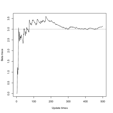
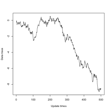
We repeat Step 1 and 2 L𝐿L times. The following Figures preset the simulation results. Figures 4 and 4 are traces of data 𝐗N=(XtjN)j=1Nsubscript𝐗𝑁superscriptsubscriptsubscript𝑋superscriptsubscript𝑑𝑗𝑁𝑗1𝑁\mathbf{X}_{N}=(X_{t_{j}^{N}})_{j=1}^{N} and Ξ²^jNsuperscriptsubscript^𝛽𝑗𝑁\hat{\beta}_{j}^{N} at l=100𝑙100l=100, respectively (l(≀L)annotated𝑙absent𝐿l(\leq L) denote each steps of Monte Carlo trials). y𝑦y-axis has update times j≀N𝑗𝑁j\leq N. The dotted line in Figure 4 denotes the true value Ξ²0=3subscript𝛽03\beta_{0}=3. In Figure 4 we plot (j,Ξ²^jNΒ―)𝑗¯superscriptsubscript^𝛽𝑗𝑁(j,\overline{\hat{\beta}_{j}^{N}}) for j≀N𝑗𝑁j\leq N, where

Ξ²^jNΒ―:=1Lβ€‹βˆ‘l=1LΞ²^jN,l,assignΒ―superscriptsubscript^𝛽𝑗𝑁1𝐿superscriptsubscript𝑙1𝐿superscriptsubscript^𝛽𝑗𝑁𝑙\displaystyle\overline{\hat{\beta}_{j}^{N}}:=\frac{1}{L}\sum_{l=1}^{L}\hat{\beta}_{j}^{N,l},

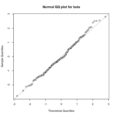
and Ξ²^jN,lsuperscriptsubscript^𝛽𝑗𝑁𝑙\hat{\beta}_{j}^{N,l} denotes the value of Ξ²^jNsuperscriptsubscript^𝛽𝑗𝑁\hat{\beta}_{j}^{N} at l≀L𝑙𝐿l\leq L. We give a QQ-plot for WN:=N/2​β02​(Ξ²^NNβˆ’Ξ²0)assignsubscriptπ‘Šπ‘π‘2superscriptsubscript𝛽02superscriptsubscript^𝛽𝑁𝑁subscript𝛽0W_{N}:=\sqrt{N/2\beta_{0}^{2}}(\hat{\beta}_{N}^{N}-\beta_{0}) in Figure 4. From the Figure 4, we expect that Ξ²^NN→𝑃β0𝑃→superscriptsubscript^𝛽𝑁𝑁subscript𝛽0\hat{\beta}_{N}^{N}\xrightarrow{P}\beta_{0} as Nβ†’βˆžβ†’π‘N\rightarrow\infty. Actually, whenever we repeat this algorithm, Ξ²^NNΒ―Β―superscriptsubscript^𝛽𝑁𝑁\overline{\hat{\beta}_{N}^{N}} nearly equal to Ξ²0subscript𝛽0\beta_{0} and standard deviations are not so large (about 0.190.190.19). We also expect that

WNβ†’β„’N​(0,1)β„’β†’subscriptπ‘Šπ‘π‘01\displaystyle W_{N}\xrightarrow{\mathcal{L}}N(0,1)

as Nβ†’βˆžβ†’π‘N\rightarrow\infty from the QQ-plot in Figure 4 since the plots almost lay on the 45 degree line.
Refer to caption
Figure 1. Trace of data 𝐗Nsubscript𝐗𝑁\mathbf{X}_{N}.
Refer to caption
Figure 2. Trace of Ξ²^jNsuperscriptsubscript^𝛽𝑗𝑁\hat{\beta}_{j}^{N}.
Refer to caption
Figure 3. Trace of Ξ²^jNΒ―Β―superscriptsubscript^𝛽𝑗𝑁\overline{\hat{\beta}_{j}^{N}}.
Refer to caption
Figure 4. QQ-plot for WNsubscriptπ‘Šπ‘W_{N}.
Acknowledgements.

The author is grateful to Professor H. Masuda, Kyushu university, for his valuable comments.

References

  • [1] V.Β S. Borkar. Stochastic approximation. Cambridge University Press, Cambridge; Hindustan Book Agency, New Delhi, 2008. A dynamical systems viewpoint.
  • [2] A.Β Dvoretzky. Stochastic approximation revisited. Advances in Applied Mathematics, 39:1327–1332, 1968.
  • [3] V.Β Fabian. On asymptotic normality in stochastic approximation. The Annals of Mathematical Statistics, 39:1327–1332, 1968.
  • [4] V.Β Fabian. On asymptotically efficient recursive estimation. The Annals of Statistics, 6(4):854–866, 1978.
  • [5] J.Β Jacod, A.N.Β Shiryaev. Limit theorem for stochastic processes. Springer–Verlag Berlin, New York, 1987.
  • [6] Y.Β A. Kutoyants. Statistical inference for ergodic diffusion processes. Springer Series in Statistics. Springer–Verlag London, Ltd., London, 2004.
  • [7] N.Β Lazrieva, T.Β Sharia, and T.Β Toronjadze. Semimartingale stochastic approximation procedure and recursive estimation. Journal of Mathematical Sciences, 153(3):211–261, 2008.
  • [8] M.B.Β Nevel’son, R.Z.Β Khas’minskii Stochastic approximation and recursive estimation. Providence, RI: American Mathematical Society, 1973.
  • [9] H.Β Robbins, S.Β Monro A stochastic approximation method. The Annals of Mathematical Statistics, 400–407, 1951.
  • [10] T.Β Sharia. On the recursive parameter estimation in the general discrete time statistical model. Stochastic Processes and their Applications, 73(2):151–172, 1998.
  • [11] T.Β Sharia. Rate of convergence in recursive parameter estimation procedures. Georgian Mathematical Journal, 14(4):721–736, 2007.
  • [12] T.Β Sharia. Recursive parameter estimation: convergence. Statistical Inference for Stochastic Processes, 11(2):157–175, 2008.
  • [13] T.Β Sharia. Recursive parameter estimation: asymptotic expansion. Annals of the Institute of Statistical Mathematics, 62(2):343–362, 2010.