Cosmological test using strong gravitational lensing systems
Abstract
As one of the probes of universe, strong gravitational lensing systems allow us to compare different cosmological models and constrain vital cosmological parameters. This purpose can be reached from the dynamic and geometry properties of strong gravitational lensing systems, for instance, time-delay of images, the velocity dispersion of the lensing galaxies and the combination of these two effects, . In this paper, in order to carry out one-on-one comparisons between CDM universe and universe, we use a sample containing 36 strong lensing systems with the measurement of velocity dispersion from the SLACS and LSD survey. Concerning the time-delay effect, 12 two-image lensing systems with are also used. In addition, Monte Carlo (MC) simulations are used to compare the efficiency of the three methods as mentioned above. From simulations, we estimate the number of lenses required to rule out one model at the confidence level. Comparing with constraints from and the velocity dispersion , we find that using can improve the discrimination between cosmological models. Despite the independence tests of these methods reveal a correlation between and , could be considered as an improved method of if more data samples are available.
keywords:
gravitational lensing - Galaxy - cosmology: dark energy1 Introduction
Detailed study of type Ia supernovae (Riess et al., 1998; Perlmutter et al., 1999) has revealed that our universe is undergoing an era of accelerating expansion, which suggests the composition of our universe may include some unknown components such as dark energy. Observations from other independent methods such as cosmic microwave background (CMB), baryon acoustic oscillations (BAO), clusters of galaxies, gamma-ray bursts (Wang et al. 2015) and large-scale structure can lead to the same result. The cosmological constant is considered to be the best candidate of dark energy, which is accordant with many observations (Riess et al., 2004; Davis et al., 2007; Kowalski et al., 2008; Wang et al., 2011; Wang & Dai, 2014). However, there are many other models that were proposed to explain the observations, one promising model is model (Melia, 2007; Melia & Shevchuk, 2012; Yu & Wang, 2014). The existence of so many theoretical models calls for more precise and complementary data to differentiate between the models.
Since Walsh et al. (1979) discovered the strong gravitational lensing in Q0957+561, strong gravitational lensing has become one powerful probe in the study of cosmology (Zhu, 2000; Chae, 2003; Chae et al., 2004; Mitchell et al., 2004; Zhu & Sereno, 2008; Zhu, 2008) and astrophysics, i.e., measuring the mass of galaxies or clusters. Up to now, hundreds of lensing systems produced by galaxies or quasars have been discovered, but only one part of them with geometry and dynamic information can be used for statistical analysis. The observations of about 70 lensing systems provide the data required not only for studying the statistical properties of galaxy structures and mass distribution (Ofek et al., 2003; Chae & Mao, 2003), but also for confining cosmological parameters. The Einstein radius obtained from the deflection angle and the time-delay of different images can provide the information of angular diameter distance (i.e. and ) independently, and further can be used to constrain cosmological models.
In recent years, many tests based on strong gravitational lensing have been used to constrain cosmological parameters. For example, the statistical data in Cosmic Lens All-Sky Survey (CLASS) demonstrated assuming a flat cosmology and non-evolving galaxy populations (Chae, 2003). Assuming a mean galaxy density profile that does not evolve with redshift, a -dominated cold dark matter cosmology, and Gaussian distributions for bulk parameters describing the lens and source populations, Dobke et al. (2009) found a sample of 400 time-delay lenses can reach the similar levels of precision as from the best of other methods. Coe & Moustakas (2009) presented the first analysis of time-delay lenses to constrain a broad range of cosmological parameters. Using the 80 data from various gravitational lens survey and lensing galaxy cluster with X-ray observations and optical giant luminous arcs, Cao et al. (2012) obtained in the CDM model. The application of selection methods in one-on-one comparisons between CDM and Universe has found that the former is favored by the data (Melia et al., 2015). In their simulations of velocity dispersion , in order to rule out at the confidence level assuming the cosmology is CDM, they found about 200 lens systems are required, while a sample of at least 300 systems to rule out CDM if the background is . Similar results were obtained in the simulations of (Wei et al., 2014). However, Paraficz & Hjorth (2009) argues that is more effective to constrain cosmological parameters than and separately.
In this paper, we focus on constraining cosmological parameters using observational data of and in a sample containing 36 lensing and a sample of 12 time-delays. In addition, we perform one-on-one comparisons between the model and the CDM model through MC simulations of , and to estimate the number of data points needed to rule out one model in the background of another at the confidence level. To achieve this goal we assume the three methods are independent and the dependence tests are performed later.
The paper is organised as follows. In the next section, we introduce the strong gravitational lensing systems as the probe of the universe. In section 3, we test the CDM and models utilising the measured data samples. In section 4, we use MC simulations of , and the combination independently to perform one-on-one comparisons. We also compare the capability of these three methods and test their independence. Conclusions and discussions are given in section 5.
2 Strong Lenses as a Probe of the Universe
In this paper, we mainly concern two cosmological models: the CDM and the models. In the CDM model, angular diameter depends on several parameters, including Hubble constant , density fractions , and , where , and are current matter, radiation, dark energy densities respectively, and is critical density of our universe. Assuming a zero spatial curvature universe, we have . The angular diameter distance between redshifts and is given by the formula
| (1) |
Since radiation is insignificant at gravitational lensing redshifts and noting , we have two essential parameters needed to be constrained, including and . In the model (Melia, 2007; Melia & Shevchuk, 2012), there is only one parameter in the angular diameter distance
| (2) |
Strong gravitational lensing occurs when the observer, the lens and the source are well aligned that we can get separate images of the source due to the gravitational field of the lens. The time-delay is caused by the difference in length of the optical paths and the gravitational time dilation for the ray passing through the effective gravitational potential of the lens . For a given image at angle position with the source position at angle , time delay can be written as (Blandford & Narayan 1986)
| (3) |
where is the redshift of the lens, are the angular diameter distances between observer and lens, observer and source, and lens and source, respectively. If the lens geometry and the effective gravitational potential of the lens are known, we can define the time-delay distance
| (4) |
If such systems have only two images at and , the time delay is given by the expression
| (5) |
under the single isothermal sphere (SIS) model.
Another method to constrain cosmological models is to use the Einstein radius in the SIS model,
| (6) |
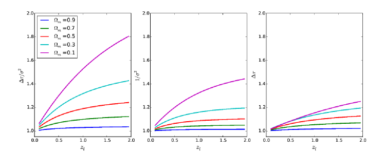
which varies with cosmological models via the ratio of angular diameter distances between lens/source, and observer/source. From equations (3) and (4), we can see that time-delay is proportional to and the square of the velocity dispersion is proportional to . The ratio is determined only by , that is to say,
| (7) |
We show the relations between the redshift of lens and the three quantities in the equation (7) in CDM model with a fixed source redshift . In Figure 1, we plot these quantities in several cases relative to the Einstein-de Sitter Universe () as in Paraficz & Hjorth (2009). The extent of separations between curves in Figure 1 reveals the sensitivity of the corresponding method to discriminate cosmological models. Comparing with constraints from and the velocity dispersion , we find that using can significantly improve the discrimination between cosmological models. Meanwhile, the sensitivity increases with the redshift of lens, thus, it is of special significance to study high-redshift lenses.
For simplicity, we still follow the approximation in Paraficz & Hjorth (2009) that and . From equations (5) and (6), we obtain
| (8) |
Up to now, we have three methods: velocity dispersion , time delay and the combination . The relations between these quantities and angular distances can be found in equations (5), (6) and (8). Equations about strong gravitational lensing in our paper are based on the SIS model. However, Treu et al. (2006) found that the ratio between the velocity dispersion of the lensing galaxy and the velocity dispersion for the corresponding singular isothermal sphere or ellipsoid, , is close to unity. Here, we assume .
3 Samples and results
3.1 Samples Used
In consideration of the consistency with a simple power-law (or even SIS) profile, SIS lens should have only 2 images (Biesiada et al., 2010, 2011), thus we use 36 lenses which have only two images in sample I for Einstein ring data. All lenses in our sample had well measured central dispersions taken from the SLACS and LSD surveys (Biesiada et al., 2010; Bolton et al., 2008; Newton et al., 2011). We use time-delay lenses to compare cosmological models as well. In our paper, 12 time-delay lensing systems are contained in sample II.
For each model, we find the best fit by minimizing the function
| (9) |
where and for Einstein circle lenses (ECL) and time-delay lenses (TDL), respectively. In function, donates the variance of and it can be obtained from the error propagation formula of . Thus, the standard deviation of from Einstein circle lensing is
| (10) |
and we take error both for (Grillo et al. 2008) and . The standard deviation of time-delay can be written as
| (11) |
Here, we also introduce the parameter , to represent the derivation from the SIS model.
3.2 Cosmological Models Test
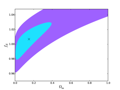
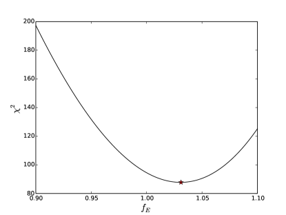
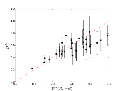
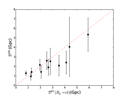
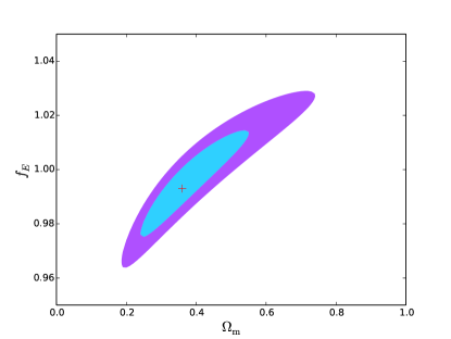
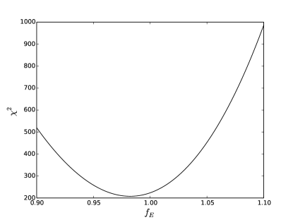
At first, we use 36 lenses in sample I (summarised in Table 1) to compare CDM with Universe. In this case, there are two free parameters ( and ) in CDM and one parameter () in model. Using sample I, we find the minimum =45.6 for , in the CDM. For the Universe, the best fit is at 1 confidence level. The results are shown in Figure 2. In order to compare the constraints, the relation between and for the best-fitting parameters is shown in Figure 3. Using 36 lensing systems we find the values for both CDM and are high. Obviously, the parameters are not well constrained. The primary reason is that the number of data points is too small to yield a good constraint.
| System | (arcsec) | Refs | |||
|---|---|---|---|---|---|
| SDSS J0037-0942 | 0.1955 | 0.6322 | 1.47 | 1 | |
| SDSS J0216-0813 | 0.3317 | 0.5235 | 1.15 | 1 | |
| SDSS J0737+3216 | 0.3223 | 0.5812 | 1.03 | 1 | |
| SDSS J0912+0029 | 0.1642 | 0.3239 | 1.61 | 1 | |
| SDSS J1250+0523 | 0.2318 | 0.795 | 1.15 | 1 | |
| SDSS J1630+4520 | 0.2479 | 0.7933 | 1.81 | 1 | |
| SDSS J2300+0022 | 0.2285 | 0.4635 | 1.25 | 1 | |
| SDSS J2303+1422 | 0.1553 | 0.517 | 1.64 | 1 | |
| CFRS03.1077 | 0.938 | 2.941 | 1.24 | 1 | |
| HST 15433 | 0.497 | 2.092 | 0.36 | 1 | |
| MG 2016 | 1.004 | 3.263 | 1.56 | 1 | |
| SDSS J0955+0101 | 0.1109 | 0.3159 | 0.91 | 2 | |
| SDSS J0959+4416 | 0.2369 | 0.5315 | 0.96 | 2 | |
| SDSS J1143-0144 | 0.106 | 0.4019 | 1.68 | 2 | |
| SDSS J1205+4910 | 0.215 | 0.4808 | 1.22 | 2 | |
| SDSS J1403+0006 | 0.1888 | 0.473 | 0.83 | 2 | |
| SDSS J1403+0006 | 0.1888 | 0.473 | 0.83 | 2 | |
| SDSS J0044+0113 | 0.1196 | 0.1965 | 0.79 | 2,3 | |
| SDSS J0330-0020 | 0.3507 | 1.0709 | 1.1 | 2,3 | |
| SDSS J0935-0003 | 0.3475 | 0.467 | 0.87 | 2,3 | |
| SDSS J1112+0826 | 0.273 | 0.6295 | 1.49 | 2,3 | |
| SDSS J1142+1001 | 0.2218 | 0.5039 | 0.98 | 2,3 | |
| SDSS J1204+0358 | 0.1644 | 0.6307 | 1.31 | 2,3 | |
| SDSS J1213+6708 | 0.1229 | 0.6402 | 1.42 | 2,3 | |
| SDSS J1218+0830 | 0.135 | 0.7172 | 1.45 | 2,3 | |
| SDSS J1432+6317 | 0.123 | 0.6643 | 1.26 | 2,3 | |
| SDSS J1436-0000 | 0.2852 | 0.8049 | 1.12 | 2,3 | |
| SDSS J1443+0304 | 0.1338 | 0.4187 | 0.81 | 2,3 | |
| SDSS J1451-0239 | 0.1254 | 0.5203 | 1.04 | 2,3 | |
| SDSS J1525+3327 | 0.3583 | 0.7173 | 1.31 | 2,3 | |
| SDSS J1531-0105 | 0.1596 | 0.7439 | 1.71 | 2,3 | |
| SDSS J1538+5817 | 0.1428 | 0.5312 | 1 | 2,3 | |
| SDSS J1621+3931 | 0.2449 | 0.6021 | 1.29 | 2,3 | |
| SDSS J2238-0754 | 0.1371 | 0.7126 | 1.27 | 2,3 | |
| Q0957+561 | 0.36 | 1.41 | 1.41 | 4 | |
| MG1549+3047 | 0.11 | 1.17 | 1.15 | 5 | |
| CY2201-3201 | 0.32 | 3.9 | 0.41 | 6,7,8 |
| System | (arcsec) | (arcsec) | (days) | Refs | ||
|---|---|---|---|---|---|---|
| B0218+357 | 0.685 | 0.944 | 0.057 0.004 | 0.280 0.008 | +10.5 0.2 | 1,2,3 |
| B1600+434 | 0.414 | 1.589 | 1.14 0.075 | 0.25 0.074 | -51.0 2.0 | 4,5 |
| FBQ0951+2635 | 0.26 | 1.246 | 0.886 0.004 | 0.228 0.008 | -16.0 2.0 | 6 |
| HE1104-1805 | 0.729 | 2.319 | 1.099 0.004 | 2.095 0.008 | +152.2 3.0 | 2,7,8 |
| HE2149-2745 | 0.603 | 2.033 | 1.354 0.008 | 0.344 0.012 | -103.0 12.0 | 6,9 |
| PKS1830-211 | 0.89 | 2.507 | 0.67 0.08 | 0.32 0.08 | -26 5 | 10,11 |
| Q0142-100 | 0.49 | 2.719 | 1.855 0.002 | 0.383 0.005 | -89 11 | 6,12 |
| Q0957+561 | 0.36 | 1.413 | 5.220 0.006 | 1.036 0.11 | -417.09 0.07 | 13,14 |
| SBS 0909+532 | 0.83 | 1.377 | 0.415 0.126 | 0.756 0.152 | +45.0 5.5 | 6,15 |
| SBS 1520+530 | 0.717 | 1.855 | 1.207 0.004 | 0.386 0.008 | -130.0 3.0 | 6,16 |
| SDSS J1206+4332 | 0.748 | 1.789 | 1.870 0.088 | 1.278 0.097 | -116 5 | 17 |
| SDSS J1650+4251 | 0.577 | 1.547 | 0.872 0.027 | 0.357 0.042 | -49.5 1.9 | 6,18 |
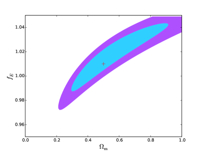
In addition, we use 12 time-delay lensing systems in sample II (summarised in Table 2) to compare these two models using . In the CDM model, there are three parameters () and two parameters () in Universe to be constrained. From maximizing the likelihood function
| (12) |
we obtain the best-fitting parameters: in the CDM model and in the model. Here, we marginalize in the CDM model to find the confidence levels in plane,
| (13) |
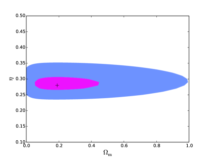
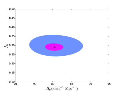
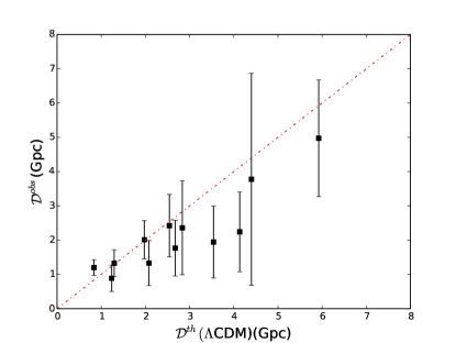
where is the probability distribution of . Figure 4 presents the constraints on plane and plane. Similar as in the Einstein circle lensing systems test, we compare and in Figure 5.
To compare two models using Einstein circle lenses, we calculate the reduced , which is defined as the ratio of the minimum of and the degree of freedom. The degrees of freedom are for CDM and for . Thus, we obtain and . Now, the difference in between these two models is not big enough to provide strong evidence which model is better than another. In the time-delay lensing test, we use the Akaike Information Criterion, , where is the maximum likelihood and is the number of free parameters (Liddle, 2007). For the model , i.e. and CDM respectively) with , the likelihood can be written as
| (14) |
Then we get , , and . So the likelihood of being correct is and for CDM, the corresponding probability is . In order to rule out one model at a confidence level, samples containing more data points are required.
4 MC simulations with a Mock Sample
We make one-on-one comparisons between CDM and using three different observed quantities (, and ) under the assumption that these methods are independent. In our paper, we estimate the number of lenses needed by using different methods to rule out another model at the confidence level. From the values of , and in observed lensing data, in our simulations, the redshift of sources are equally distributed between to and the lens redshift between to . In the first method (using ), we assume the velocity dispersions are uniformly distributed from to (Paraficz & Hjorth, 2009). Then we infer from equation (6) with . We assign the uncertainty of to be . Since the simulated sample contains a large number of data points, the Bayes Information Criterion () is more appropriate
| (15) |
where and are the number of data points and free parameters (Schwarz, 1978). The form of the likelihood here is similar with equation (14), where is substituted by . Then, we estimate the number of data points needed to rule out one model (i.e. ) using another model (i.e. CDM) as the background universe.
In the simulations of time-delay lensing systems (using ), we assume the time-delays are uniformly distributed between -150 to 150 days and we then infer from equation (5). We assume the uncertainty of is . In the simulations of the combination of and , the distributions of and are same with the first two methods and is inferred from equation (8). We still assign the uncertainty of to . The parameters to be constrained in different models and methods are summarized in Table 3. We assume and for the CDM background and the background, respectively.
| Method | Model | Free parameters | Degree of freedom |
|---|---|---|---|
| CDM | 2 | ||
| 1 | |||
| CDM | 2 | ||
| 1 | |||
| CDM | 2 | ||
| 1 |
Since is the mutual parameter in three different methods, in order to differentiate these methods, we study the constraints on using 200 simulated data points in both CDM and backgrounds. This simulation is repeated for 1000 times to find the statistical distributions of the best-fitting .
One general concern is whether the method is independent with the other methods since it is derived from and . We will discuss this issue in the subsection 4.3.
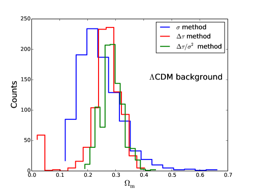
4.1 CDM Background Cosmology
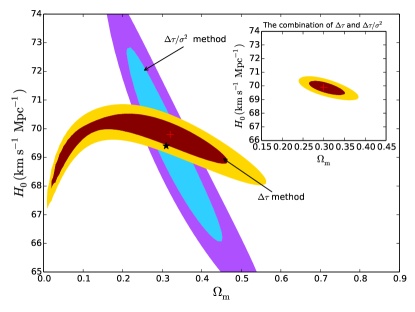
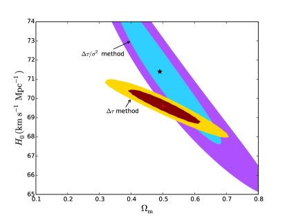
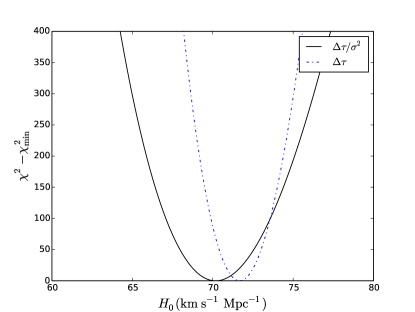
In this case, we assume the background universe is CDM and seek for the least number of data points needed to rule out at a confidence level. We find samples of 300, 200 and 150 data points are needed utilising , and respectively. The constraints on parameters and are listed in Table 4. The and confidence regions for CDM model in plane for the method and plane for both and methods are illustrated in Figure 6. In figure 7, we show the distribution for parameters ( and ) in the model.
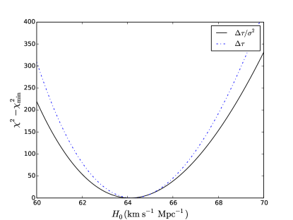
From Table 4 we find that a sample of less data points is needed using the method comparing with the methods of and . From Figure 6, we find that the constraints on different parameters vary with methods. For example, the method of is more favorable to constrain the Hubble constant (), while can constrain better. The cross between the contour plots of the method and in Figure 6 shows that the combination of these two methods can give tighter constraints on both and . This conclusion can be confirmed from the inset of Figure 6 (right) with the best fitting parameters: , . A credible comparison between three different methods can be obtained from our 1000 repetitive simulations. In this simulation, each sample for these methods contains 200 simulated data points and we run 1000 minimizations for each method respectively. The distributions of optimal are shown in Figure 8. In order to differentiate these three methods quantitatively, we use normal distribution function to fit the distributions of optimal and we find the FWHMs are 0.157, 0.093 and 0.084 for the methods of , , respectively. Thus the constraint on using is tighter than other two methods.
| Method | Model | Best-fitting parameter | |
|---|---|---|---|
| () | CDM | 339 | |
| 357 | |||
| CDM | 238 | ||
| 256 | |||
| CDM | 169 | ||
| 187 |

4.2 Background Cosmology
We find that a sample of 200 data points for the method or 600 data points for the method or for the combined method is needed independently to rule out the CDM model in the background. The results of constraints are listed in Table 5.
| Method | Model | Best-fitting parameters | |
|---|---|---|---|
| () | CDM | 249 | |
| 238 | |||
| CDM | 670 | ||
| 664 | |||
| CDM | 134 | ||
| 125 |
In Figure 9, we illustrate the and confidence regions for CDM model in plane for the method and plane for both and methods. In figure 10, we show the distributions of and in model.
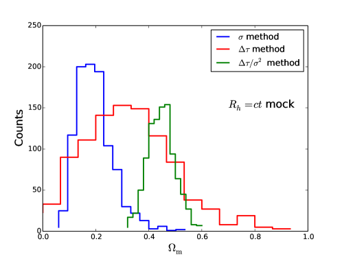
Similar conclusions can be obtained in the background. We also repeat our simulations for 1000 times to differentiate the constraints on utilising three different methods, the distributions are illustrated in Figure 11 (normal fitting FWHMs are 0.143, 0.402 and 0.122 for the methods of , , respectively). Noting that a larger sample (of 600 data points) is needed using the method and the FWHM is obviously larger than other methods. We can draw the conclusion that is poorly constrained using , which is consistent with the constraint of in Figure 4 (left). In addition, another difference is that CDM contains more degrees of freedom to fit the data.
4.3 Independence Tests for , and
The previous discussions in this section are based on the assumption that these three methods are independent. This assumption is appropriate to differentiate the efficiency of different methods. However, when we put the method into practical cosmological tests, we must consider its independence on the other two methods. Here, independence tests are performed using MC simulations and the steps are given as follows.
(i) Generate two samples (200 data points in each sample) for and the methods using the previous scheme in the beginning of this section assuming the background is CDM. The lensing redshifts () of the corresponding data points in each sample should be the same, so as .
(ii) In this step we generate the sample for the method. Here, , time-delay and velocity dispersion can be obtained directly from the samples in step (i). Noting that and , can be expressed in the form That means we can combine the three samples as one with the measurement of both time-delay, velocity dispersion, and .
(iii) Using the samples generated in (i) and (ii) to constrain and obtain the optimal for these three methods.
(iv) Repeat steps (i)-(iii) times (here, =500) and get three samples of optimal for the methods of , and respectively.
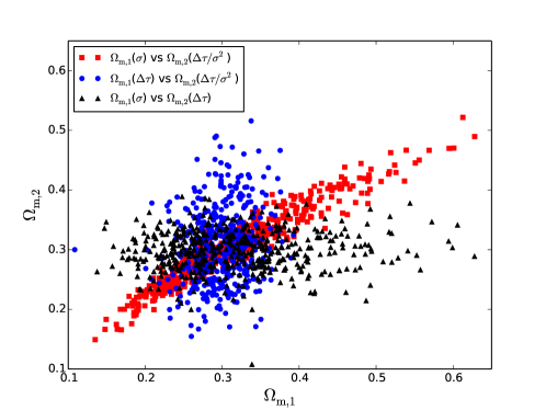
Figure 12 shows the correlations of the obtained samples. The -axis is the sample of obtained from one method while -axis is the sample of obtained from another method, for instance, (the method) versus (the method). From Figure 12 we find the samples of optimal obtained from and are strongly and positively correlated, which means that resultant from the method and the method of are not independent. Besides, this figure illustrates that there is no obvious correlation between and , and . Despite the independence tests of these methods revealing a correlation between and , could be considered as an improved method of , especially for the lensing systems with the measurement of both time-delays, velocity dispersions and the radii of two images ( and ).
5 Conclusions and discussions
In this paper, we use three methods to constrain cosmological parameters and make one-on-one comparisons between CDM Universe and Universe. Using sample I containing 36 two-image Einstein circle lenses, we find the current two-image data set failed to rule out one Universe at the confidence level. In addition, we use a sample of 12 time-delay lensing systems to compare CDM and . By using Akaike Information Criterion we find is superior to CDM with a likelihood of . More data points are required to rule out one model at a higher confidence level.
Since lack of gravitational lensing systems observed with both , and , the sample for can merely be obtained through simulations. Therefore, we use MC simulations to compare different methods concerning velocity dispersion , time-delay and their combination, , in one-on-one comparisons. Through assuming a background universe, we try to find the least number of data points to rule out another cosmological model at a confidence level. From the distributions of optimal we find that the is superior to in the constraints of .
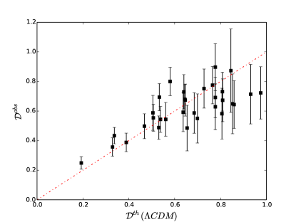
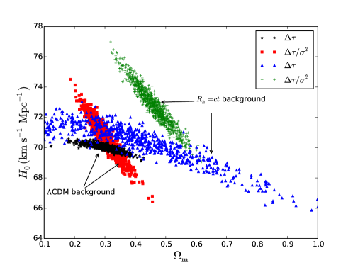
In order to differentiate the efficiency of different methods, we repeat our simulations for 1000 times to compare the constraints on utilising three different methods. In the simulation, we assign the number of data points in each sample to be 200. For both backgrounds, we find that can give a tighter constraint on than and . As shown in Figure 13, we plot the best-fit data points in plane for and methods. The only difference of in CDM Universe and Universe backgrounds is the shift of the best-fitting and . However the distribution of optimal obtained through in the Universe background is more diffuse compared with CDM background. This can explain that the sample needed in the method of in the background is much larger than in the CDM background (600 data points versus 200 data points).
These three methods are useful to compare cosmological models and each of them has its advantages in special aspects. Although and are not independent, it can be considered as an improved method of . Besides, from our independence tests we find that the method and are independent, thus the joint consideration of them can be used to give a tight constraint in plane for CDM model. Despite the relative lack of observational data, future studies of lensing systems and high resolution observations of galaxies will provide more geometry and dynamic information about strong gravitational lenses. Then, the method will become a powerful method in cosmological model selections.
Acknowledgements
We thank Shun-Sheng Li for fruitful discussions and careful reading of the manuscript. This work is supported by the National Basic Research Program of China (973 Program, grant No. 2014CB845800) and the National Natural Science Foundation of China (grants 11422325, 11373022, J1210039 and 11033002), the Excellent Youth Foundation of Jiangsu Province (BK20140016). C.C.Y is also supported by Innovation Program of Undergraduates, Ministry of Education of China under Grant No. S1410284047.
References
- Auger et al. (2008) Auger M. W. et al., 2008, ApJ, 673, 778
- Biesiada et al. (2010) Biesiada M., Piorkowska A., Malec M., 2010, MNRAS, 406, 1055
- Biesiada et al. (2011) Biesiada M., Malec M., Piorkowska A., 2011, RAA, 11, 641
- Blandford & Narayan (1986) Blandford R., Narayan R., 1986, ApJ, 310, 568
- Bolton et al. (2008) Bolton A. S. et al., 2008, ApJ, 682, 964
- Burud et al. (2002) Burud I. et al, 2002, A&A, 383,71
- Cao et al. (2012) Cao S. et al., 2012, JCAP, 03, 016
- Carilli et al. (1993) Carilli C. L., Rupen M. P., Yanny B., 1993, ApJ, 412, L59
- Chae & Mao (2003) Chae K. H., Mao S., 2003, ApJ, 599, L61
- Chae (2003) Chae K. H., 2003, MNRAS, 346, 746
- Chae et al. (2004) Chae K. H. et al., 2004, ApJ, 607, L71
- Coe & Moustakas (2009) Coe D., Moustakas, L. A., 2009, ApJ, 706, 45
- Colley et al. (2003) Colley W. N. et al., 2003, ApJ, 587, 71
- Dai & Kochanek (2005) Dai X., Kochanek C. S., 2005, ApJ, 625, 633
- Dai & Kochanek (2009) Dai X., Kochanek C. S., 2009, ApJ, 692, 667
- Davis et al. (2007) Davis T. M. et al., 2007, ApJ, 666, 716
- Dobke et al. (2009) Dobke B. M. et al., 2009, MNRAS, 397, 3ll
- Falco et al. (1997) Falco E. E. et al., 1997, ApJ, 484, 70
- Grillo et al. (2008) Grillo C., Lombardi M., Bertin G., 2008, A&A, 477, 397
- Jackson et al. (1995) Jackson N. et al., 1995, MNRAS, 274, L25
- Kochanek et al. (2008) Kochanek C. S. et al, 2008, available at http://www.cfa.harvard.edu/castles/
- Koopmans & Treu (2002) Koopmans L.V.E., Treu T., 2002, ApJ, 568, L5
- Koopmans & Treu (2002) Koopmans L., Treu T., 2003, ApJ, 583, 606
- Koptelova et al. (2002) Koptelova E. et al., 2012, A&A, 544, A51
- Kowalski et al. (2008) Kowalski M. et al., 2008, ApJ, 686, 749
- Lehar (1993) Lehr J. et al., 1993, ApJ, 105, 847
- Lehr (2000) Lehr J. et al., 2000, ApJ, 536, 584
- Liddle (2007) Liddle A. R., 2007, MNRAS, 377, L74
- Lovell et al. (1998) Lovell J.E.J. et al, 1998 ApJ, 508, L51
- Melia (2007) Melia F., 2007, MNRAS, 382, 1917
- Melia & Shevchuk (2012) Melia F., Shevchuk A. S. H., 2012, MNRAS, 419, 2579
- Melia et al. (2015) Melia F., Wei J. J., Wu X. F., 2015, AJ, 149, 2
- Meylan et al. (2005) Meylan G. et al., 2005, A&A, 438, L37
- Mitchell et al. (2004) Mitchell J. L., Keeton C. R., Frieman J. A., Sheth R. K., 2004, ApJ, 622, 81
- Newton et al. (2011) Newton E. R. et al., 2011, ApJ, 734, 104
- Ofek et al. (2003) Ofek E. O., Rix H. W., Maoz D., 2003, MNRAS, 343, 639
- Paraficz & Hjorth (2009) Paraficz D., Hjorth J., 2009, A&A, 507, L49
- Perlmutter et al. (1999) Perlmutter P et al., 1999, ApJ, 517, 565
- Poindexter et al. (2007) Poindexter S. et al., 2007, ApJ 660 146
- Riess et al. (1998) Riess A. G. et al., 1998, Astron.J. 116, 1009
- Riess et al. (2004) Riess A. G. et al., 2004, ApJ. 666, 716
- Schwarz (1978) Schwarz G., 1978, Ann. Statist., 6, 461
- Treu & Koopmans (2004) Treu T., Koopmans L.V., 2004, ApJ, 611, 739
- Treu et al. (2006) Treu T., Koopmans L. V., Bolton A. S., Burles S., Moustakas L. A., 2006, ApJ, 640, 662
- Vuissoz et al. (2007) Vuissoz C. et al., 2007, A&A, 464, 845
- Wang & Dai (2014) Wang F. Y., Dai Z. G., 2014, PRD, 89, 023004
- Wang et al. (2015) Wang F. Y., Dai Z. G., Liang E. W., 2015, New Astr. Rev., 67, 1
- Wang et al. (2011) Wang F. Y., Qi S., Dai Z. G., 2011, MNRAS, 415, 3423
- Walsh et al. (1979) Walsh D. et al., 1979, Nature 279, 381
- Wei et al. (2014) Wei J. J., Wu X. F., Melia F., 2014, ApJ, 788, 190
- Wucknitz et al. (2004) Wucknitz O., Biggs A. D., Browne I.W.A., 2004, MNRAS, 349, 14
- Wisotzki et al. (1993) Wisotzki L. et al., 1993, A&A, 287, L15
- Young (1980) Young P. et al., 1980, ApJ, 241, 507
- Yu & Wang (2014) Yu H., Wang F. Y., 2014, EPJC, 74, 3090
- Zhu (2000) Zhu Z. H., 2000, Mod. Phys. Lett. A, 15, 1023
- Zhu (2000) Zhu Z. H., 2000, Int. J. Mod. Phys.D, 9, 591
- Zhu & Sereno (2008) Zhu Z. H., Sereno, M. 2008, A&A, 487, 831
- Zhu (2008) Zhu Z. H., 2008, Astron. Astrophys, 483, 15