Discrete Stochastic Models in Continuous Time for Ecology

Abstract

This article shows how to specify and construct a discrete, stochastic, continuous-time model specifically for ecological systems. The model is more broad than typical chemical kinetics models in two ways. First, using time-dependent hazard rates simplifies the process of making models more faithful. Second, the state of the system includes individual traits and use of environmental resources. The models defined here focus on taking survival analysis of observations in the field and using the measured hazard rates to generate simulations which match exactly what was measured.

1 Introduction

Discrete stochastic models in continuous time are the simplest way to turn survival analysis of an ecological system into a simulation of that system. They build models most faithful to a picture of individuals making choices which affect each other. This article describes how rules for individual behavior can construct a simulation of a population. It argues that, within the context of discrete stochastic simulation, hazard rates for transitions are intrinsic descriptions of individual behavior.

Discrete stochastic models in continuous time are associated with the Gillespie algorithm and its variants, including the Next Reaction algorithm. The Gillespie algorithm samples to find the next state and time of a stochastic process. The process and sampling algorithm are separate. This article won’t define a new sampling algorithm but will examine the stochastic process that is sampled.

Almost every discrete stochastic model in continuous time used for ecology is based upon a chemical kinetics model. These chemical kinetics models take the form of chemical species which interact according to stoichiometry at rates specified by propensities. They have been enormously successful for ecological applications such as stochastic movement models[1, 2, 3, 4] and any model that builds group behavior from individual behavior[5, 6, 7]. Clear statement of chemical kinetics as a process leads to clear specification of chemical kinetics models as matrices and vectors in Systems Biology Markup Language and computer code which, in turn, leads to their utility to solve common problems.

The chemical kinetics model constrains expression of ecological problems in two ways. The first is that every state in a chemical kinetics model is a count of chemical species when an ecologist might want the state of an individual to carry properties that record its life history. The second is that propensities are usually simple rates when an ecologist might want rates to be time-dependent, so that an insect gets more hungry over time, or a cow waits to reproduce again, or a frog jumps quickly if it jumps early. These two important modifications are that individuals hold state and their hazard rates for change are time-dependent.

Two particular areas are ripe for use of non-constant hazard rates and hazard rates more specific to individual histories. The first is stochastic movement models, which already have a strong history[1, 2, 3, 4]. The second is infectious processes. Recent studies show that while constant hazards for infection model well the most intense parts of outbreaks any analysis of early outbreaks and the distribution of early outbreaks will find incorrect $R_{0}$ if they do not include Gamma-distributed or Weibull-distributed recovery times[8, 9].

The statistical process defined in this article includes the ability for individuals to have state associated with them and the ability for hazard rates to be time-dependent, and it is called long-lived competing processes (llcp). While it is known that the Gillespie algorithm can sample such an llcp process, the process, itself, has not been specified. Lacking a specification, previous uses of time-dependent hazards and property-carrying state have misunderstood both how models relate with observation and how to sample the trajectory from such a model. The bovine viral diarrhea models of Viet et al.[10] demonstrate how time-dependent hazards can include farm management decisions within a continuous-time model, but they also mistakenly parameterize transitions in the model from holding times instead of hazard rates, both of which are explained in the results section below. The wasp model of Ewing et al.[11] calculates competition among behavioral drives, including temperature dependence, using a detailed continuous-time model with time-dependent hazards, but the sampling method used is statistically biased. In both cases, the resulting trajectories are biased, so that summary data, such as average survival, are incorrect. Correctness here is a question of whether observation times and theoretical rates put into a model are the same that come out of simulation of the model. Correctness is a question of whether the statistical machinery fails the effort required to gather data and parameterize a model.

The other consequence of lacking a specification is that there are no ready tools with which to construct a discrete stochastic process in continuous time which has time-dependent hazard rates. A mathematical specification is the first step to understanding how to state a process clearly in a file or in code, such that it can be sampled. It was the goal of the authors to make construction of ecological and epidemiological models trustworthy and rapid.

The central tenet of the stochastic processes defined in this article is that individuals compete. Not only do individuals compete, but also for a single individual, the drive to eat, the drive to reproduce, and the drive to move compete. For these models, an individual is the sum of its drives. Each of those drives is modeled by a separate stochastic process whose hazard rate comes from survival analysis. The long-lived competing process is built from a set of conditionally-independent stochastic processes, conditional on interruption by other processes. Each process has its own time-dependent hazard to fire.

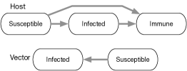
Figure 1: A simple compartmental model showing a vector infecting a host.

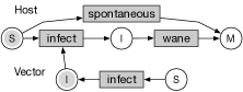
Figure 2: This diagram emphasizes transitions between states because each transition is associated with a stochastic process. Host states label susceptible, infected, and immune. Vector state label susceptible and infected.

To understand the aptness of a competing process formulation take a classic compartmental diagram, such as the vector and host model in Fig. 1, shows which state transitions are possible for an individual. This diagram, given rates for transitions, could guide construction of a differential equation model for a population, but think here modeling individual behaviors. The diagram in Fig. 2 represents rules for how an individual can change state from one compartment to another and at what rate the state can change. It emphasizes possible transitions from which move those individuals from one compartmental state to the next. Sec. 3.3 shows how to make this diagram into a specification for a model in the same way that a stoichiometric matrix is a specification for a chemical model.

The methods section of this article and appendix construct a representation of a statistical process in order to show generality and completeness. The results section covers how to construct and parameterize this process.

2 Previous Work

This article defines a class of stochastic processes without discussing the algorithms with which to sample trajectories of those processes. These algorithms are commonly known as Gillespie-type and encompass the following: Direct, Direct non-Markovian, First Reaction, Next Reaction, Anderson’s Next Reaction[12, 13, 14, 15]. This article doesn’t extend these algorithms but rather expands the possible ways to define changes of state, given Gillespie-type dynamics in time.

While the exposition within this article relies on calculus of stochastic variables, a more modern approach to discussion of Markov renewal processes uses martingales and random time changes, as described by Anderson and Kurtz[16]. Restricting mathematical development to calculus is more approachable but will falter to answer more precise questions about what it means for a competing process to be well-defined.

There is a mathematical identity that any discrete, stochastic, continuous-time process can be rewritten as a set of competing processes, one for each possible next state and defined anew at each time step[17, 18]. The long-lived competing processes described below are an extension of competing processes to encompass biological behaviors which aren’t reset each time anything in the system changes, as happens for competing processes. It can be considered a subset of an older technique called the Generalized Semi-Markov Process (gsmp), used in engineering[19]. The main criticisms of gsmp simulations are that they can be complicated to specify and slow to simulate. Restriction of the long-lived competing processes to conform to Markov renewal processes reduces complexity somewhat and greatly speeds computation by making possible the use of Next Reaction method.

The Generalized Stochastic Petri Net (gspn) in Sec. 3.3 is not only a data structure but also a set of engineering techniques for building a process using that data structure[20, 21]. Those rules are more amenable to human-mediated processes and are a superset of what is described here. This article focuses on simulation as enactment of estimations from survival analysis, so it skips over much of the extensive feature set, and complication, associated with use of gspn in manufacturing and reliability analysis.

There have been major frameworks designed and used for general individual-based modeling in ecology. The devs discrete-event simulation is a general-purpose simulation tool adopted for ecology[22]. Later groups made tools more focused on ecological simulation in order to reduce the burden of programming and design. osiris and wesp are good examples[23, 24]. Both focused on ease-of-use and correctness by combining higher-level abstraction with software architecture.

In contrast to these frameworks, the work presented here is a simpler mathematical model. There is a sample implementation as a C++ library, and references to data structures and algorithms are sufficient to implement the model[25]. The emphasis, however, is on how to join statistical estimation of a system with its simulation because understanding causal dependence of a system is more complicated than programming, and quantitative understanding begins with statistical correctness.

3 Methods

3.1 Markov Renewal Process

To call a simulation a discrete stochastic process in continuous time, means that it is a representation of a Markov renewal process (mrp). Take the mrp as the definition of what it means to be such a simulation. The structure of an mrp determines in what way a model approximates the real world. It also circumscribes limitations on what choices in a simulation conform to mathematical requirements. The mrp is well-known and this exposition follows Çinlar[26] in order to explain how all of the actions of every individual in a simulation, taken together, form one single mrp from which to sample trajectories.

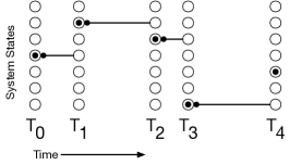
Figure 3: A Markov renewal process defines a probability distribution of a next state at a next time given the current state. Each circle represents a different state of the system. Each arrow is a transition to a next state and time. From now, what is next?

For an mrp, time is a random variable, so it jumps from an initial time, $T_{0}$, to the next time, $T_{1}\geq T_{0}$. For any jump, from $T_{n}$ to $T_{n+1}$, the state of the system is defined at those times, not in-between. The times themselves form a countable set. The state of the system, $X_{n}$, is, itself, a random variable on a discrete space, so it is labeled $X_{n}=i$.

The central engine of an mrp is that the next state and the next time are chosen according to a joint probability for the next state to be state $X_{n+1}=j$ at time $T_{n+1}$ given current state $X_{n}=i$ and time $T_{n}$,

$$P\left[X_{n+1}=j,T_{n+1}-T_{n}\leq t|X_{n}=i\right].$$ (1)

The density of this probability, its derivative, is called the semi-Markov kernel, denoted $q_{ij}(T_{n+1}-T_{n})$. A process which conforms to an mrp specifies all the next possible states of the system, and, given the current state, the joint probability of each next state and time for that state.

An mrp is a view of an ecological simulation, zoomed out so that anything that happens, in any part of the simulation, is the next change to the state of the whole simulation, as shown by the states in Fig. 4. Saying that a complex simulation is an instance of an mrp is a statement that all of the biological and physical processes within a simulation become a single statistical process, marching forward in time, according to a single joint probability distribution. Identification of that joint probability distribution is what permits uniform sampling in a simulation.

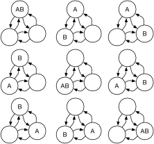
Figure 4: Given a system with two individuals, A and B, which can move among three metapopulations, there are nine physical states of the system, as shown. Because the mrp can depend on times in a state, the complete state of the system, $X_{n}$, can include the times at which A and B arrived in their current configuration.

There is no restriction for an mrp that the probability distribution for the next states be exponential. For every Markov random process, the next state depends only on the system state $X_{n}$ at $T_{n}$. For a Markov random process whose distribution of next stopping times is always exponential, the probability of arrival at a particular next state not only doesn’t depend on states before $X_{n}$ but also doesn’t depend on the amount of time the system takes to arrive at that next state.

The exposition here treats the state space, $X_{n}$, as a finite set of states, which would be restrictive in practice. The number of states can be infinite as long as the next possible states, $X_{n+1}=j$ can be sampled statistically. Çinlar’s careful presentation allows states to be real numbers, explaining that, given a discrete set of stopping times, the set of real numbers chosen to be stopping times is itself a finite set.

A process which conforms to an mrp must define a set of initial states, a set of next states given any current state, and a joint probability for the next states and times at which they might occur. The next section constructs such a process, starting with intuition for competing processes.

3.2 Long-lived Competing Processes

The guiding idea for constructing this specific mrp is that individuals compete for resources and modify the environment. There will be multiple simultaneous stochastic processes, each of which represents a tendency towards changing the individual or the environment. Definition of long-lived competing processes (llcp) proceeds in two steps, defining the state of the overall system, and showing how to calculate the probability of the next state and time, Eq. 1, from current state.

Figure 5: Long-lived competing processes define individual actions which, together, create a Markov renewal process. Only one long-lived process fires at a time. Others may be enabled or disabled when one fires, but at no other time. There isn’t a one-to-one association between a competing process and the state of the system. Each process modifies the joint substates of the system in some known way to cause a change in the current state.

The state of a system with many individuals, such as the metapopulation in Fig. 6, is exponentially large (the number of trajectories given an initial value will be combinatorially large). Any time any one of the individuals moves, sthe whole system is in a new state, $X_{n+1}=j$. The total number of states is the number of arrangements of individuals, and times at which they could arrive at those arrangements. A goal of this the llcp specification is to ensure that the behavior of any particular individual can depend on only a local environment. Whether its local environment is its location or the its neighboring individuals, that individual’s behavior will be independent of any behavior that doesn’t interfere with its local environment.

The physical state of the system is the state of individuals and their environment, separate from times at which the system entered this physical state. This definition follows the language of the gsmp in Glynn[19]. It is specified as a set of substates, $s_{0},s_{1},\ldots s_{p}$, so that those substates can represent the local environment of an individual. This could be the location of each individual or nearby food, for example. The substates are a disjoint set which, together, describe the whole physical state of the mrp.

Each possible cause for change in the system is represented by a separate stochastic variable, $L_{m}$. For instance, “individual two jumps down” would be a single cause for change. At the moment the individual arrives in a spot, the cause to jump away from that spot is called enabled at time $T_{m}^{e}$. That cause may fire, or a competing cause may disable it. For instance, the firing of “individual two jumps right” would prevent that individual from having jumped North.

The probability for a cause to fire at any time depends on some subset, $\{s_{i}\}$, of the substates of the physical system and can always be written as a cumulative distribution function defined by a time-dependent hazard rate, $\lambda_{m}(t)$,

$$P\left[L_{m}\leq T_{m}|\{s_{i}\}\right]=1-\exp\left[-\int_{T_{m}^{e}}^{T_{m}}\lambda_{m}(s)ds\right].$$ (2)

This is the probability for the time at which a particular cause will happen, were it to happen. It is defined, not since the last transition, but in absolute time, since the start of a simulation. Associated with this cause is a rule for when it is enabled, when it is disabled, and what it does to the substates when it fires. Those three rules are functions of the substates associated with this cause and no other physical substates.

Figure 6: The same metapopulation simulation of A and B moving among three locations could be modeled with three physical substates, one for each metapopulation, and six processes which compete to move an individual to neighboring metapopulations. The competing processes are enabled only when a substate has individuals to move.

Figure 7: Long-lived competing processes are defined in absolute time since the start of the simulation because they represent what is allowed within a model. When a long-lived competing process is enabled, it has nonzero hazard. When it fires or becomes disabled, the hazard returns to zero.

A simulation defines many causes simultaneously. From all of these causes, the first to fire determines what happens next in the system. The next time, $T_{n+1}$, for the whole system as an mrp is the minimum of the set of stochastic variables,

$$T_{n+1}=\mbox{min}\left(\{L_{m}\}\right),$$ (3)

taking into account that none of the enabled causes fired before $T_{n}$. It’s a competition to be the first to fire, determined by the cause-specific probabilities for firing. When one fires, it may disable or enable other causes. The cause that fires determines how the system changes to a new state, $X_{n+1}=j$. Multiple causes may independently effect the same new state, in which case they, together, define the all-causes probability of that state. The joint probability for $X_{n+1}$ and $T_{n+1}$ is given in appendix A.

No cause that is competing, in the sense that the firing of another cause could disable it, will ever fire with the probability distribution given in Eq. 2. However, the long-lived competing process guarantees that the hazard rate of a cause, as determined by standard survival analysis, will match the hazard rate of Eq. 2, because the hazard rate is the rate at which a cause will fire, were it to fire. To define an llcp,

• Define physical substates, $s_{0},s_{1},\ldots s_{p}$,

• For each cause, define

  • An enabling function on the substates which determines enabling and, if enabled, returns the stochastic variable, $L_{m}$, and

  • A firing function, which modifies substates.

• Substates and causes form an undirected, bipartite graph.

Haas covers the possibility of incomplete distributions for a similar process, the gsmp[21]. If there is some chance that the biological process associated with a cause might never happen, even in the absence of competition, then the probability in Eq. 2 will be incomplete, meaning it will not sum to one. Only if there is some probability that no cause in the system fires, so that the simulation stops entirely, will the probability of Eq. 1 be incomplete. Most often it will sum to one or be zero entirely when the system reaches what is called an absorbing state. In an ecological simulation, an absorbing state could mean all individuals are recovered from disease, or it could be a delicate way to say every individual has died.

A consequence of this construction of an llcp is that the enabling times, $T_{m}^{e}$, for the long-lived processes become part of the state of the system. For simple Markov processes, as opposed to mrps, those enabling times don’t affect the choice of the next state but, in general, they are important for non-exponential distributions. While the times are real-valued, the state of the system is discrete because those times are drawn from the set of times, $T_{n}$, at which the system is defined.

Within an llcp, no two long-lived processes may fire simultaneously. For instance, no two causes could both have distributions in time which fire exactly at $5\>\mbox{pm}$. It is possible to define a more elaborate process which accounts for such conflict, but it would not as clearly obey hazard rates from survival analysis and would require a sampling mechanism more complicated than Gillespie-type.

It is possible to define an infinite number of physical states and even an infinite number of possible transitions (for instance, an ant wandering on sand), as long as the number of enabled transitions is finite after each time step. The restriction is that it must be possible to sample the central probability, Eq. 1. Computationally, this would require storing only that part of the state that is currently relevant to the simulation.

The long-lived competing process, as a pure expression of simulation by survival analysis, can be seen as a stripped-down version of the Generalized Semi-Markov Process (gsmp). The main historical criticism of gsmp is that such arbitrary definition of what is a substate and when causes are enabled or disabled produces a slow simulation. However, solution for the next time step, Eq. 3, is exactly what Gillespie’s algorithm solves, and the tremendous speedup from Gibson and Bruck’s Next Reaction Method relies on recording which causes depend on which physical states. Those two details are what make an llcp more computable than an arbitrary continuous-time stochastic system.

3.3 Generalized Stochastic Petri Net

A Generalized Stochastic Petri Net (gspn) is a family of stochastic processes and associated data structures. This section defines a long-lived competing process using the data structure and associated nomenclature of gspn. Being specific about the data structure creates a clear relationship between the firing of a process and how the state of the system as a whole changes.

The state of a system, excluding its transitions, is defined by tokens at places, much like the location of checkers on a board defines the state of a game. Each place has a unique identifier. The tokens at a place are a physical substate, $s_{i}$, of the llcp. While chemical kinetics simulations usually describe only a count of molecules of a species, individuals in an ecological simulation will often have more life history, such as birth times or subspecies, which can be represented as properties of a token.

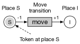
Figure 8: The language of the gspn is that a transition moves tokens among places. The cardinality of the moving tokens is stoichiometry. Each token may have properties, which means it may contain state within the token. This graph, accompanied by a list of properties of the token and transition, is a specification of a simulation.

Transitions move and modify tokens, which is called firing a transition to produce an event. The enabling rule and firing rule all obey stoichiometry, which is a count of how many tokens are taken from a place or put to a place when a transition fires. This isn’t required for the llcp but has been shown by Haas to produce an equivalent statistical process[21]. If tokens do not have properties, then stoichiometry can be sufficient to describe both enabling and firing rules. A transition is enabled when the number of tokens at its inputs meets or exceeds its required inputs. It is disabled when this is no longer true. A transition, upon firing, moves the requisite number of tokens from inputs to outputs.

When tokens have properties, as they often will for ecological simulation, then the specification for each transition may be augmented with a rule such as, there must be at least one input token with the property that the individual is older than three weeks. Hazard rates for firing may be parameterized on properties of any tokens at transition inputs.

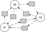
Figure 9: A movement model for a single individual moving among three habitats might have six transitions. Coefficients on edges indicate the number of tokens a transition needs to be enabled and where a transition moves tokens when it fires, much like stoichiometry in chemical systems.

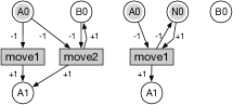
Figure 10: The stoichiometry of a gspn requires movement of tokens. Shown here are two different ways to implement a metapopulation movement model which incorporates movement dependence on population size. The gspn on the left defines a separate transition for each configuration of occupancies. The transition “move2” defines a hazard for moving individual A when individual B is present. The gspn on the right creates a separate place whose token count represents the number of individuals in the metapopulation. This extra state avoids combinatoric explosion of the number of transitions.

The state of the system is not only the tokens, with their properties and locations, but also the set of enabling times for transitions. Because this model permits non-constant hazard rates, the enabling times are necessary to know the distribution of future firing times for the system of transitions.

To define a gspn,

• Define a set of places.

• Define tokens which can move among those places and may have properties.

• Each transition has

  • An enabling function which returns whether the transition is enabled on its places and returns the stochastic variable for the firing time of this transition.

  • A stoichiometric coefficient specifying how many tokens are taken from or sent to each place upon firing.

  • A firing function which moves and modifies properties of tokens.

• Places and transitions form a bipartite graph which is directed by stoichiometry.

The gspn is a network in that transitions connect to places which connect to other transitions. For most simulations, this network can be created as a graph structure with marking at the places and transition enabling times at the transitions. The data on this graph is then the state of the model. How a simulation chooses what to fire next is separate from the state of the model, and any one of the Gillespie algorithms would yield the same ensemble of results.

4 Results

This section discusses rational construction of such a stochastic process from real-world observations or from mental models of ecological processes. Consistency with the outside world can be subtle anywhere in a model that two individuals might make conflicting decisions, which is the point of greatest interest.

4.1 Choice of States

An early step in building a model is to decide what can be the states of the system. The granularity of a model is a measure of how many behaviors are grouped together. For instance, an individual-based model of movement might include each wandering ungulate, whereas a more coarse-grained model could represent a single state for the location of a whole herd.

The term “compartmental model” comes from the task of distinguishing types of tissue in microscope images. The task is assignment of a continuous observable to a discrete class. A state in a gspn can be tied to a differentiating observation or to a theoretically relevant tipping point, such as survival of a metapopulation past early stochastic die-off. Something as simple as a state that represents a location still involves choice. For instance, a movement model of butterflies going bush to bush might identify a state according to the nearest bush, but it might identify a state as the last bush on which the butterfly landed, even if the butterfly has since taken off from that bush. The latter choice would correspond to field observations which record times at which insects land.

The second step is to choose how tokens on places represent those states. The combination of token and place together define the state. A movement model could have a place for each location, or it could store the current place as a property of an individual’s token. Both choices are valid, but a gspn which has fewer transitions connecting to the same place tends to be more efficient for simulation. Two transitions which depend on the same place equate to two biological processes which depend on the same local environment. They are coupled, and that coupling means a simulation has to do more work to ensure the currency of each process when shared state changes.

However states are chosen, the choice of which states to define combines with the ecological reality of which transitions among states are possible to create a necessary set of transitions to parameterize.

4.2 Holding Times and Waiting Times

The behaviors of an individual become a set of related transitions in a gspn. Consider an example of an individual which arrives at a metapopulation and can move to one of four other metapopulations. There are four transitions, one for each movement, and all have the same enabling time, the moment the individual arrived at its starting location. A token starts in one place, and each transition, were it to fire, would move it to a different place. Together, four transitions define the movement behavior of a single individual.

There are two questions to answer about such a system: what happens next and when it happens. These together are the joint probability of Eq. 1 which is $P[\mbox{what},\mbox{when}]$. As with any joint probability, there are two factorizations. These factorizations are called the holding time and the waiting time.

The holding time formulation asks, given what happens next, when will it happen? This factorizes the joint probability as $P[\mbox{what}]P[\mbox{when}|\mbox{what}]$. Two quantities together specify the density of this distribution, the time-independent stochastic probability density, $\pi_{ij}$, of one outcome or the other, and the time-dependence of when that outcome happens, $h_{ij}(T-T_{e})$, given that it will happen. This latter quantity is called the holding time. Time for a distribution is measured as time since enabling, which is time since the token arrived at the current place.

The waiting time formulation asks, given when the next event happens, what will happen? This factorizes the joint probability as $P[\mbox{when}]P[\mbox{what}|\mbox{when}]$. The density of times for the next event are called the waiting time, $w_{i}(T-T_{e})$. This information, were it observed by itself in an experiment, would be insufficient to determine hazard rates for transitions. It must be augmented by the time-dependent stochastic probability, $\pi_{ij}(T-T_{e})$, which asks the probability of one outcome or another at the given firing time.

Neither the holding time nor the waiting time are what go into the gspn. Given measurement or specification of holding times or waiting times, survival analysis reduces them to hazard rates, $\lambda_{ij}(T-T_{e})$, which are the probability per unit time that an event happens, given that it has not yet happened. It is this hazard rate that specifies the distribution of a transition in Eq. 2. For the simple example of a token moving to one of some number of places, the hazard rate can be found from the semi-Markov kernel written either as $q_{ij}(T-T_{e})=\pi_{ij}h_{ij}(T-T_{e})$ or as $q_{ij}(T-T_{e})=w_{ij}(T-T_{e})\pi_{ij}(T-T_{e})$. From that kernel, the hazard rate is

$$\lambda_{ij}(T-T_{e})=\frac{q_{ij}(T-T_{e})}{1-\sum_{j}\int_{T_{e}}^{T}q_{ij}(s)ds}.$$ (4)

This simplified analysis of an individual’s choices in the presence of an environment provides states and hazards with which to construct a system of many individuals sharing an environment. For observed data, a statistical estimator, such as Nelson-Aalen or Kaplan-Meier, construct hazards and integrated hazards which properly account for the kind of censoring that looks, in a gspn, like one transition disabling another transition[27].

The hazard rate for every transition can be stated equivalently by a transition distribution, $f(t)=\lambda(t)\exp(-\int\lambda(s)ds)$. The holding time, waiting time, and transition distribution are three different probability densities in time. Mistaking holding time distributions for transition distributions will construct a gspn whose timing isn’t what was measured or estimated. If and only if a transition can never be disabled by another transition, so that it is independent of all other transitions, will this probability distribution be the same as the holding time which will, in turn, be the same as the waiting time. In all interesting cases, they differ.

Construction of a stochastic, continuous-time model can be a balancing act because observed rates for transitions, the holding or waiting times, are the result of competition among individuals and other ecological processes, whereas simulation is controlled by hazard rates. Consequently, a simulation constructed from seemingly reasonable choices of hazard rate may show transition rates above or below expectations because of dependency among transitions as they compete. If some transition rates are estimated or inferred, they may be reparameterized. The common technique of establishing a parameter which is a scaling factor on the transition distribution may not be desirable because it scales hazard rate in a time-dependent way and because it changes how incomplete the transition is. Incompleteness implies a transition would never fire, even in the absence of competition, which may not be an intended consequence of rescaling.

4.3 Markovian Systems

The chemical kinetic models that are most commonly used for ecology and epidemiology are Markovian, which implies that every transition’s distribution is exponential. Exponential distributions have the unique property that the hazard rate is constant from the enabling time onward, so that once a transition is enabled, it is no longer important to remember when it was enabled. A gspn model whose transitions are all exponentially-distributed therefore need not include enabling times in its state.

Consider two individuals in the same location of a metapopulation model. One gspn representation represents their presence in a location by two tokens on two places. Transitions can move those tokens to the other locations. If both have identical transition rates for moving to other locations, then an alternative representation in a gspn is to place both tokens at the same place. The transition’s hazard rate is then the sum of the hazard rates of each token, but, at the moment the transition fires, it picks only one token to move. When all hazard rates are constant, this technique of coalescing multiple places and transitions into one place and one transition can greatly speed computation. It also works, however, for time-dependent hazard rates, as long as all coalesced hazard rates have the same time dependence, with the same enabling time.

While an llcp on a gspn and a Markovian chemical kinetic model both use exponential distributions, the llcp permits more general rules for when transitions are enabled and how state changes when it fires.

4.4 Model as a Graph

No particular representation of a model as places, tokens, and transitions is unique. There can always be another model with different places, tokens or transitions whose trajectory is one-to-one equivalent. For instance, we might represent a single insect as a token hopping among places, or we might represent it as a token with a property which is its current location. Nevertheless, the form of these models, as graphs whose nodes can be enumerated and cataloged, offers a unique chance to construct models incrementally and compare results.

Given a particular gspn representation of a model, every aspect of the model is cataloged as a place, transition, or marking. When comparing another, similar model, some of the places, transitions and markings will be the same, and some will be different. It is possible to make a list which can be verified computationally. This is a significant improvement over more free-form code.

Composition of models becomes composition of graphs. This might be a hierarchical composition, as when individuals with disease states are composed by a contact graph, or it could be a composition of an ecological model with an economics model. In either case, modular composition of Petri Nets by transition fusion or place fusion is already described[28, 29]. Graph fusion techniques offer a formal method for joining gspn.

The gspn graph itself encodes causal dependency in a simulation. Connections between transitions and places form a bipartite graph. Enforcement of stoichiometry means that every transition takes tokens from input places and gives tokens to output places, so that edges of this graph are directed. Any transition whose firing would disable another transition makes that other transition dependent. Stoichiometry records when removing a token disables a transition, so it encodes this statistical dependency. The converse statement is that transitions whose parent places are not shared cannot be dependent.

The most immediate advantage of a clear dependence structure is computational efficiency. Because the directed bipartite graph limits possible causes and effects of any firing transition, the same graph enables efficient implementation of Gibson and Bruck’s Next Reaction algorithm or Anderson’s method, which is an equivalent algorithm based on hazard rates. Both of these optimizations of Gillespie’s First Reaction method augment the stochastic process described here with added state describing a remaining integrated hazard for sampling each transition. Maintenance of this state imposes a requirement carefully ensured for long-lived competing processes, that any transition whose hazard rate or enabling changes when another transition fires must be dependent on that transition. For the gspn, this means it must stoichiometrically share an input place with the transition’s output places. An alternative implementation could separate this dependency list into its own directed graph among transitions.

5 Conclusions

Chemical kinetics simulations with exponentially-distributed transitions are well understood and commonly in use for ecology. The addition of time-dependent hazards and more general firing rules, as described here, introduces significantly more complexity for theory and implementation, but it allows design of simulations which more accurately obey both measurement and intuition. Individual behavior is neither measured nor imagined as happening at constant rates, so the ability to model with time-dependent hazard rates avoids the more complicated question of what behavior a simulation represents.

By offering a definition of an underlying stochastic process, this article sets ground rules so that it becomes possible to focus on ecological questions about a simulation. One complaint about individual-based models is that the only specification for complex models is code[30, 31], and specification of an llcp is entirely separate from the code used to sample the process. Since hazard rates are central to simulation of an llcp, survival analysis for complex systems becomes crucial. Techniques borrowed from survival analysis, such as proportional hazards and frailty models, provide known tools for estimation of parameters for a simulation.

As noted in Grimm et al, a simulation requires a hierarchy of choices[7]. The stochastic process supports choice of who or what is included in the simulation and, above that, the behaviors under study. These, in turn, are mirrored in layers of software. The authors provide a sample implementation of llcp as a C++ library[25]. This, in turn, supports construction of an application which expresses an ecological model. The llcp is a statistical process upon which to build modeling tools more focused on specific tasks, such as animal movement, epidemiology, and metapopulation analysis.

The authors thank David J. Schneider and Christopher R. Myers for helpful discussions. This work was supported by the Science & Technology Directorate, Department of Homeland Security, via interagency Agreement No. HSHQDC-10-X- 00138.

Appendix A Derivation of Long-lived Competing Processes

In order to affix notation, we define the continuous probability distribution of a non-negative, real-valued random variable $X$, denoted $F_{X}(T)$, as $F_{X}(T)=\mathcal{P}[X\leq T]$. Given that $F_{X}(T$ is sufficiently smooth, its density is the derivative, $f_{X}(T)=dF_{X}(T)/dT$. The survival is the complement of the probability distribution, $G_{X}(T)=1-F_{X}(T)$. Lastly, the hazard rate is the ratio of density to survival, $\lambda_{X}(T)=f_{X}(T)/G_{X}(T)$. The hazard rate specifies the density

$$f_{X}(T)=\lambda_{X}(T)\exp\left[-\int_{0}^{T}\lambda_{X}(s)ds\right]$$ (5)

for differentiable probability distributions. Subject to the caveat of differentiability, there is no loss of generality in describing stochastic processes in terms of hazards.

A long-lived competing process defines a physical state $s_{i}$, composed of substates, $s_{i}=(p_{0},p_{1},\ldots)$. There are stochastic variables, $L_{k}$, defined in absolute time, $T$, since the start of the simulation. The system state, $J_{n}$, consists of both the physical state, $s_{i}$, and the enabling times of each of the $L_{k}$. The stochastic variables, their enabling rules, and their firing rules, form an operator on the state of the system. This operator, distinct from an initial state, is the model for all of what can happen in a simulation.

At the moment of enabling a competing process, the survival distribution has the expected form, $G_{L_{k}}(T)=\mathcal{P}[L_{k}>T]$. Once any process has fired, those $L_{k}$ which remain enabled are now known not to have fired, so their probability distributions are rescaled. Defining a long-lived competing process by its hazard rate, the rescaled survival distribution integrates over future times,

$$G_{L_{k}}(T,T_{0})=\exp\left[-\int_{T_{0}}^{T}\lambda_{L_{k}}(s)ds\right],$$ (6)

where $T_{0}$ is the current time of the last observed event. Each of these $L_{k}$ has a density defined in terms of its hazard in absolute time, $f_{L_{k}}(T)=\lambda_{L_{k}}(T)\exp\left[-\int_{T_{0}}^{T}\lambda_{L_{k}}(s)ds\right]$ The joint density for these independent processes is their product, $f(T)=\Pi_{k}f_{L_{k}}(T_{k})$.

The probability at time $T_{n-1}$ of any next state, $J_{n}$ and time $T_{n}$ is a question of which of the $L_{k}$ fires first and when it fires. The time at which a particular process would fire, were it first to fire, corresponds to integrating the joint density over all ways in which every other process can fire later,

$$q_{ij}(T)=\int_{T_{n}}^{\infty}\cdots\int_{T}^{\infty}\Pi_{k}f_{L_{k}}(s_{k})ds_{k},$$ (7)

where the integrals are over all but one of the stochastic processes. This quantity is called the semi-Markov density and, in terms of hazard rates, integrates to

$$q_{ij}(T)=\lambda_{L_{k}}(T)\exp\left[-\int_{T_{n-1}}^{T}\sum_{k}\lambda_{L_{k}}(s)ds\right].$$ (8)

The semi-Markov density, $q_{ij}(T)$, is a joint discrete and continuous probability density. It will be incomplete if any of the stochastic variables $L_{k}$ are incomplete. This joint probability distribution can be split two ways into a marginal and conditional. Integrating the semi-Markov kernel over all time yields a stochastic matrix, $\pi_{ij}=\int_{T_{n-1}}^{T}q_{ij}(s)ds$, which is the marginal probability of choosing a cause associated with a particular $L_{k}$. If all causes which lead to the same final state are grouped together, then $p_{ij}$ is the usual stochastic matrix used to determine the next state of the system. The conditional of $p_{ij}$ is called the holding time, $h_{ij}(T)=q_{ij}(T)/p_{ij}$. This is the probability distribution for firing of a cause given that this cause will be the next to fire. Confusion of $h_{ij}(T)$ and $f_{L_{k}}(T)$ will lead to trajectories which do not match input values. The other marginal distribution is the waiting time until the next event, $w_{ij}(T)=\sum_{j}q_{ij}(T)$, obtained by summing over all causes which are enabled. The marginal for this is a time-dependent stochastic matrix, $p_{ij}(T)=q_{ij}(T)/w_{ij}(T)$.

References

- Patterson et al. [2008] T. A. Patterson, L. Thomas, C. Wilcox, O. Ovaskainen, J. Matthiopoulos, State-space models of individual animal movement, Trends in Ecology & Evolution 23 (2) (2008) 87–94, ISSN 0169-5347, URL http://www.ncbi.nlm.nih.gov/pubmed/18191283.
- Choquet et al. [2011] R. Choquet, A. Viallefont, L. Rouan, K. Gaanoun, J.-M. Gaillard, A semi-Markov model to assess reliably survival patterns from birth to death in free-ranging populations, Methods in Ecology and Evolution 2 (4) (2011) 383–389, ISSN 2041210X, URL http://doi.wiley.com/10.1111/j.2041-210X.2011.00088.x.
- Nathan et al. [2008] R. Nathan, W. M. Getz, E. Revilla, M. Holyoak, R. Kadmon, D. Saltz, P. E. Smouse, A movement ecology paradigm for unifying organismal movement research, PNAS 105 (49).
- Durrett and Levin [1994] R. Durrett, S. A. Levin, Stochastic Spatial Models: A User’s Guide to Ecological Applications, Philosophical Transactions of the Royal Society B: Biological Sciences 343 (1305) (1994) 329–350, ISSN 0962-8436, URL http://rstb.royalsocietypublishing.org/cgi/doi/10.1098/rstb.1994.0028.
- Gables and Deangelis [2014] C. Gables, D. L. Deangelis, Individual-Based Modeling of Ecological and Evolutionary Processes, Annual Review of Ecology, Evolution, and Systematics 36 (2005) (2014) 147–168.
- Huston et al. [1988] M. Huston, D. Deangelis, W. Post, New Models Unify Ecological Theory: Computer simulations show that many ecological patterns can be explained by interactions among individual organisms, BioScience 38 (10) (1988) 682–691.
- Grimm and Railsback [2005] V. Grimm, S. F. Railsback, Individual-based Modeling and Ecology, Princeton University Press, 2005.
- Yan [2008] P. Yan, Separate roles of the latent and infectious periods in shaping the relation between the basic reproduction number and the intrinsic growth rate of infectious disease outbreaks, Journal of theoretical biology 251 (2) (2008) 238–52, ISSN 1095-8541, URL http://www.ncbi.nlm.nih.gov/pubmed/18191153.
- Dunn et al. [2013] J. M. Dunn, S. Davis, A. Stacey, M. A. Diuk-Wasser, A simple model for the establishment of tick-borne pathogens of Ixodes scapularis: a global sensitivity analysis of R0, Journal of Theoretical Biology 335 (2013) 213–21, ISSN 1095-8541, URL http://www.ncbi.nlm.nih.gov/pubmed/23850477.
- Viet et al. [2004] A.-F. Viet, C. Fourichon, H. Seegers, C. Jacob, C. Guihenneuc-Jouyaux, A model of the spread of the bovine viral-diarrhoea virus within a dairy herd, Preventive veterinary medicine 63 (3-4) (2004) 211–36, ISSN 0167-5877, URL http://www.ncbi.nlm.nih.gov/pubmed/15158572.
- Ewing et al. [2002] B. Ewing, B. S. Yandell, J. F. Barbieri, R. F. Luck, L. D. Forster, Event-driven competing risks, Ecological Modelling 158 (2002) 35–50.
- Gillespie [2007] D. T. Gillespie, Stochastic simulation of chemical kinetics, Annual Review of Physical Chemistry 58 (2007) 35–55, ISSN 0066-426X, URL http://www.annualreviews.org/doi/abs/10.1146/annurev.physchem.58.032806.104637.
- Gillespie [1978] D. T. Gillespie, Monte Carlo simulation of random walks with residence time dependent transition probability rates, Journal of Computational Physics 28 (3) (1978) 395–407, ISSN 00219991, URL http://linkinghub.elsevier.com/retrieve/pii/0021999178900608.
- Gibson and Bruck [2000] M. A. Gibson, J. Bruck, Efficient Exact Stochastic Simulation of Chemical Systems with Many Species and Many Channels, The Journal of Physical Chemistry A 104 (9) (2000) 1876–1889, ISSN 1089-5639, URL http://dx.doi.org/10.1021/jp993732q.
- Anderson [2007] D. F. Anderson, A modified next reaction method for simulating chemical systems with time dependent propensities and delays, The Journal of Chemical Physics 127 (21) (2007) 214107, ISSN 0021-9606, URL http://www.ncbi.nlm.nih.gov/pubmed/18067349.
- Anderson and Kurtz [2011] D. F. Anderson, T. G. Kurtz, Continuous time Markov chain models for chemical reaction networks, in: Design and Analysis of Biomolecular Circuits, Springer, 3–42, 2011.
- Howard [2007] R. A. Howard, Dynamic Probabilistic Systems: Semi-Markov and Decision Processes, Dover, Mineola, NY, ISBN 9780486152004, 2007.
- Berman [1963] S. M. Berman, Note on extreme values, competing risks and semi-Markov processes, The Annals of Mathematical Statistics 34 (3) (1963) 1104–1106.
- Glynn [1989] P. Glynn, A GSMP formalism for discrete event systems, Proceedings of the IEEE 77 (1) (1989) 14–23, ISSN 00189219, URL http://ieeexplore.ieee.org/lpdocs/epic03/wrapper.htm?arnumber=21067.
- Conte et al. [1991] G. Conte, S. Donatelli, G. Franceschinis, I. Dipartimento, U. Milano, V. Moretto, C. Svizzera, An Introduction to Generalized Stochastic Petri Nets, Microelectron. Reliab. 31 (4) (1991) 699–725.
- Haas [2002] P. J. Haas, Stochastic Petri Nets: Modelling, Stability, Simulation, Springer-Verlag, New York, New York, USA, 2002.
- Zeigler and Vahie [1993] P. Zeigler, S. Vahie, DEVS Formalism and Methodology: Unity of Conception/Diversity of Application, in: Proceedings of the 1993 Winter Simulation Conference, 573–579, 1993.
- Mooij and Boersma [1996] W. M. Mooij, M. Boersma, An object-oriented simulation framework for individual-based simulations (OSIRIS): Daphnia population dynamics as an example, Ecological Modelling 93 (2) (1996) 139–153.
- Lorek and Sonnenschein [1999] H. Lorek, M. Sonnenschein, Modelling and simulation software to support individual-based ecological modelling, Ecological Modelling 115 (2-3) (1999) 199–216, ISSN 03043800, URL http://linkinghub.elsevier.com/retrieve/pii/S0304380098001938.
- Dolgert and Schneider [2014] A. J. Dolgert, D. J. Schneider, Semi-Markov Library, URL https://github.com/afidd/Semi-Markov, 2014.
- Çinlar [1975] E. Çinlar, Introduction to Stochastic Processes, Dover Publications, Inc., Mineola, NY, ISBN 978-0-486-27632-8, 1975.
- Datta and Satten [2001] S. Datta, G. A. Satten, Validity of the Aalen–Johansen estimators of stage occupation probabilities and Nelson–Aalen estimators of integrated transition hazards for non-Markov models, Statistics & Probability Letters 55 (4) (2001) 403–411, ISSN 01677152, URL http://linkinghub.elsevier.com/retrieve/pii/S0167715201001559.
- Christensen and Petrucci [2000] S. Christensen, L. Petrucci, Modular Analysis of Petri Nets, The Computer Journal 43 (3) (2000) 19.
- Gomes and Barros [2005] L. Gomes, J. Barros, Structuring and Composability Issues in Petri Nets Modeling, IEEE Transactions on Industrial Informatics 1 (2) (2005) 112–123, ISSN 1551-3203, URL http://ieeexplore.ieee.org/lpdocs/epic03/wrapper.htm?arnumber=1430654.
- Grimm et al. [2006] V. Grimm, U. Berger, F. Bastiansen, S. Eliassen, V. Ginot, J. Giske, J. Goss-Custard, T. Grand, S. K. Heinz, G. Huse, A. Huth, J. U. Jepsen, C. Jørgensen, W. M. Mooij, B. Müller, G. Pe’er, C. Piou, S. F. Railsback, A. M. Robbins, M. M. Robbins, E. Rossmanith, N. Rüger, E. Strand, S. Souissi, R. A. Stillman, R. Vabø, U. Visser, D. L. DeAngelis, A standard protocol for describing individual-based and agent-based models, Ecological Modelling 198 (1-2) (2006) 115–126, ISSN 03043800, URL http://linkinghub.elsevier.com/retrieve/pii/S0304380006002043.
- Grimm et al. [2010] V. Grimm, U. Berger, D. L. DeAngelis, J. G. Polhill, J. Giske, S. F. Railsback, The ODD protocol: A review and first update, Ecological Modelling 221 (23) (2010) 2760–2768, ISSN 03043800, URL http://linkinghub.elsevier.com/retrieve/pii/S030438001000414X.