Neutrino Sector and Proton Lifetime in a Realistic SUSY $SO(10)$ Model

Abstract

In this work I present a complete analysis of proton decay in an $SO(10)$ model previously proposed by Dutta, Mimura, and Mohapatra. The 10, $\overline{\bf{126}}$, and 120 Yukawa couplings contributing to fermion masses in this model have well-motivated restrictions on their textures intended to give favorable results for proton lifetime as well as a realistic fermion sector without the need for fine-tuning and for either type-I or type-II dominance in the neutrino mass matrix. I obtain a valid fit for the entire fermion sector for both types of seesaw dominance, including $\theta_{13}$ in good agreement with the most recent data. For the case with type-II seesaw, I find that using the Yukawa couplings fixed by the successful fermion sector fit, proton partial lifetime limits are satisfied for nearly every pertinent decay mode, even for nearly arbitrary values of the triplet Higgs mixing parameters, with only the $K^{+}\bar{\nu}$ mode requiring a minor ${\cal O}(10^{-1})$ cancellation in order to satisfy the experimental limit. I also find a maximum lifetime for that mode of $\tau(K^{+}\bar{\nu})\sim 10^{36}$ years, which should be tested by eventual experiments. For the type-I seesaw case, I find that all six pertinent decay modes of interest are satisfied for values of the triplet mixing parameters giving no major enhancement, with modes other than $K^{+}\bar{\nu}$ easily satisfied for arbitrary mixing values, and with a maximum lifetime for $K^{+}\bar{\nu}$ of nearly $10^{38}$ years.

I Introduction

It has been well-established that a certain class of $SO(10)$ Grand Unified (GUT) models minkowski are capable of elegantly solving some of the most prominent problems with the Standard Model. One of the more basic yet intriguing features of these models is the ability to naturally accommodate a right-handed neutrino, consequently allowing for a well-motivated implementation of the seesaw mechanism for neutrino mass seesaw , a long-uncontested ansatz that dynamically explains the smallness of (left-handed) neutrino masses. The seesaw was originally implemented in the framework of SUSY $SO(10)$ with only the 10- and 126-dimensional Higgs multiplets coupling to fermions rabi-aulakh ; kuo ; the 126 vev also plays the role of breaking $B\!-\!L$ and triggering the seesaw mechanism, thereby creating a deep mathematical connection between the smallness of neutrino masses and the other fermion masses. This seemingly-limited yet elegant approach yielded a realistic neutrino sector, including an accurate prediction of the value of $\theta_{13}$ goh-ng ; babu-mace , long before experiments were being done to measure its properties. This so-called “minimal” $SO(10)$ model has been explored much more thoroughly over the years by many authors with the arrival of precision measurements rabi-babu ; babu-mace ; 10-126a ; bajc ; goh-ng ; 10-126b ; fukuyama ; altarelli , and it remains a viable predictor of the neutrino sector parameters.

There are however still a number of common difficulties one faces when attempting to construct a complete and realistic candidate for unification. Furthermore, these difficulties are continually being made more severe by new experimental results, which typically manifest as new lower bounds on the possible existence of some proposed feature, as part of a disheartening streak of null results.

Arguably the most problematic feature common to nearly all GUT models arises when one examines the lifetime of the proton. In all $SO(10)$ models, heavy $SU(5)$-like gauge boson exchanges give rise to effective higher-dimensional operators that allow for

quark-lepton mixing and, consequently, nonzero probabilities for proton decay widths. Furthermore, in SUSY GUT models, several additional decay modes are available, as each of the GUT-scale Higgs superfields contains at least one colored Higgs triplet that allows for proton decay through exchange of Higgsino superpartners.

No one yet knows whether protons do in fact decay at all; so far, the lower limit on proton lifetime is known to be at least $\sim\!\!10^{32}$ years, and the partial lifetimes for the various decay modes have been continually rising through the findings of experiments superk . Thus, if any $SO(10)$ model is to be trusted, its prediction for the proton lifetime must be at least so high a number. Most minimal $SU(5)$ models have already been virtually ruled out by such limits (technically, a few niches of parameter space do still remain).

There are ways in which the proton lifetime limits can be satisfied within the framework of a given $SO(10)$ model, but doing so typically requires substantial fine-tuning to create rather extreme cancellations ($\mathrel{\vbox{\hbox{$>$}\nointerlineskip\hbox{$\sim$}}}\mathcal{O}(10^{-3})$) among the mixing parameters of the color-triplet Higgsinos exchanged in the decay. The values of those mixings cannot so far be reasonably recognized as more than arbitary free parameters, so to expect multiple instances of very sensitive relationships among them requires putting much faith in either unknown dynamics or extremely good luck. Restricting the SUSY vev ratio $v_{u}/v_{d}$, conventionally parametrized as $\tan\beta$, to small values can provide some relief without cancellation for Higgsino-mediated decay channels, but such an assumption is still ad hoc and may ultimately be inconsistent with experimental findings; hence it is strongly preferable to construct a model which is tractable for any feasible $\tan\beta$.

If however the GUT Yukawas, which are $3\!\times\!3$ matrices in generation space, have some key elements naturally small or zero, then extreme cancellations can be largely avoided by eliminating most of the dominant contributions to proton decay width. A 2013 paper by Dutta, Mimura, and Mohapatra dmm1302 proposed such a Yukawa texture for the $SO(10)$ model including a 120 coupling in addition to the 10 and $\overline{\bf{126}}$ Higgs contributions to fermion masses. The authors gave a tentative analysis of mainly leading-order relationships between key fermion fit parameters and proton partial lifetimes for a neutrino sector arising from a type-II dominant seesaw mechanism; they also provided a cursory analysis for a possible type-I solution.

The work I present in this paper verifies the initial analysis of ref. dmm1302 by $(a)$ finding a stable numerical fit to all fermion mass and mixing parameters, including the neutrino sector, where values are predictions of the model, and $(b)$ then finding adequately large lifetimes for the dominant modes of proton decay using the Yukawa couplings fixed by the fermion fit. I grounded the analysis in conservative assumptions, including large $\tan\beta$, and a comprehensive calculation relying on as few approximations as necessary. The pertinent modes of proton decay I checked for sufficient partial lifetimes are $p\rightarrow K^{+}\bar{\nu}$, $K^{0}\ell^{+}$, $\pi^{+}\bar{\nu}$, and $\pi^{0}\ell^{+}$, where $\ell=e,\mu$. I will present solutions for both type-I and II seesaw neutrino masses.

The results not only give satisfactory predictions for the neutrino sector based on corresponding charged sector fits, but also adequately predict sufficiently long-lived protons without relying on the usual large degree of cancellation. Furthermore, I find that the ansatz is completely successful in satisfying the proton lifetime limits without any need for tuning in the type-I seesaw scenario, while a modest $\mathcal{O}(10^{-1})$ cancellation is still needed in the type-II case to satisfy the partial lifetime limit of the often-problematic $p\rightarrow K^{+}\bar{\nu}$ mode. This combination of type-I and II results is precisely contrary to the tentative expectations of the authors in dmm1302 ; the discrepancy is due mainly to the unexpected significance of the effect of rotation to mass basis on the results of the decay width calculations, combined with the numerical details of the rotation matrices arising from the charged sector mass and CKM fit.

The paper is organized as follows: in section II, I give an overview of the $SO(10)$ superpotential and the fermion mass matrices following from it, followed by the details of the Yukawa texture ansatz; in section III, I expand further on the model specifics and examine general GUT proton-decay logistics in order to derive the needed partial decay widths; in section IV, I present the fermion sector results of the numerical fitting to the measured masses and mixings; in section V, I present the results of the calculation of the important partial lifetimes of the proton; and in section VI, I discuss the implications of the results and give my conclusions.

II Details of the Model

As mentioned in the introduction, the $SO(10)$ model in question has 10-, $\overline{\bf{126}}$-, and 120-dimensional Yukawa couplings contributing to fermion masses. The fields are named here as H, $\overline{\Delta}$, and $\Sigma$, respectively. Thus, the relevant superpotential terms are

$$W_{Y}\ni h_{ij}\Psi_{i}\Psi_{j}{\rm H}+f_{ij}\Psi_{i}\Psi_{j}\overline{\Delta}+g_{ij}\Psi_{i}\Psi_{j}\Sigma,$$ (1)

where $\Psi_{i}$ is the 16-dimensional matter spinor containing superfields of all the SM fermions (of one generation) plus the right-handed neutrino, and $i$ is the generation index.

After the GUT symmetry breaking, SM-type $SU(2)$ doublet representations ($\left(\,{\bf 1},{\bf 2},-\frac{1}{2}\,\right)$ + c.c ) contained in the decompositions of H, $\overline{\Delta}$, and $\Sigma$ mix with each other, and also with the doublets from 126 (which is needed to preserve SUSY invariance) and any additional fields present in the model for GUT-breaking purposes but not contributing to fermion masses, such as 210 or 54. These doublets come in pairs with conjugate SM quantum numbers, and each Higgs superfield contains one or two pairs. The mass matrix $\mathcal{M_{D}}$ for each set of doublets is determined by the couplings and vevs of the GUT-scale superpotential, and so the fields are generally expected to be heavy; however, one pair must remain light in order to play the role of the MSSM Higgs doublets $H_{u,d}$. This need requires the imposition of the fine-tuning condition $Det\,\mathcal{M_{D}}\sim 0$ (i.e., $M_{SUSY}\sim 0$ when compared to the GUT scale), which can be interpreted as the fixing of one parameter in the matrix, conventionally chosen to be the mass of the 10, $M_{H}$. This choice will have implications for proton decay analysis that I will discuss in the next section. In light of this establishment of the MSSM doublets, the effective Dirac fermion mass matrices can be written as

$${\cal M}_{u} =\tilde{h}+r_{2}\tilde{f}+r_{3}\tilde{g}$$

$${\cal M}_{d} =\frac{r_{1}}{\tan\beta}(\tilde{h}+\tilde{f}+\tilde{g})$$

$${\cal M}_{e} =\frac{r_{1}}{\tan\beta}(\tilde{h}-3\tilde{f}+c_{e}\tilde{g})$$

$${\cal M}_{\nu_{D}} =\tilde{h}-3r_{2}\tilde{f}+c_{\nu}\tilde{g},$$ (2)

where $1/\tan\beta$ takes $v_{u}\rightarrow v_{d}$ for down-type fields. Each coupling $\tilde{\lambda}_{ij}$ for $\lambda=h,f,g$ is related to $\lambda_{ij}$ from eq. (1) by an absorption of the SUSY vacuum expectation value (vev) $v_{u}$ and some function of elements of the unitary matrices $U^{\cal D}_{I\!J},\,V^{\cal D}_{I\!J}$ that diagonalize $\mathcal{M_{D}}$. These mixings are given in detail with respect to this model in olddmm and more generally in aulgarg , but those details are not relevant at this point in the discussion. The coefficients $r_{i}$ and $c_{\ell}$ are similarly defined as functions of those mixings.

The full neutrino mass matrix is determined by both Majorana mass terms in the superpotential and the Dirac mass contribution given in eq. (2). The light masses can be generally given by a combination of the type-I and type-II seesaw mechanisms, involving the vevs of both left- and right-handed Majorana terms:

$${\cal M}_{\nu}=v_{L}f-{\cal M}_{\nu_{D}}\left(v_{R}f\right)^{-1}\left({\cal M}_{\nu_{D}}\right)^{T},$$ (3)

where $v_{L,R}$ are the vevs of the SM-triplet $\overline{\Delta}_{L}$ and singlet $\overline{\Delta}_{R}$ in $\overline{{\bf 126}}$. The seesaw scale (i.e., RH-neutrino scale) coincides with the $B\!-\!L$ breaking scale and is set by $v_{R}$; typically $v_{L}\sim v_{\rm wk}^{2}/v_{R}$, although it is a free parameter of the model in principle. We will separately consider cases of type-II ($v_{L}$ term) and type-I ($1/v_{R}$ term) dominance, which can both be readily accommodated in this model. Note that the presence of the $f$ coupling in both terms intimately connects the neutrino mass matrix properties to those of the charged sector matrices, making the model quite predictive. Also note we will consider only normal mass hierarchy in this analysis.

The matrices $h$ and $f$ (with tildes or not) are real and symmetric, and $g$ is pure imaginary and anti-symmetric; hence, the Dirac fermion Yukawa couplings are Hermitian in general, and their most general forms can be written as

$$\tilde{h}=\left(\begin{array}[]{ccc}h_{11}&h_{12}&h_{13}\\ h_{12}&h_{22}&h_{23}\\ h_{13}&h_{23}&M\end{array}\right),\qquad\tilde{f}=\left(\begin{array}[]{ccc}f_{11}&f_{12}&f_{13}\\ f_{12}&f_{22}&f_{23}\\ f_{13}&f_{23}&f_{33}\end{array}\right),$$ (10)

$$\tilde{g}=i\left(\begin{array}[]{ccc}0&g_{12}&g_{13}\\ -g_{12}&0&g_{23}\\ -g_{13}&-g_{23}&0\end{array}\right).$$ (14)

$M\equiv h_{33}\sim m_{t}$ is singled out to stress its dominance over all other elements. The three matrices as written have a total of 15 parameters; taken in combination with $v_{L}$ as well as the vev and mixing ratios $r_{i}$ and $c_{\ell}$, the model has a total of 21 parameters. Correspondingly, there are in principle 22 measurable observables, including all masses, mixing angles, and CP violating phases, associated with the physical fermions, although the three PMNS phases and one neutrino mass are yet to be observed. Therefore we would prefer then to have no more than 18 parameters in the model, and generally speaking fewer parameters indicates greater predictability.

Furthermore, as I will discuss in more detail shortly, the $d=5$ effective operators that arise in proton decay are $\sim\lambda_{ij}\lambda_{kl}$ (again $\lambda=h,f,g$); therefore, increasing the number of $\lambda_{ij}$ that are small or zero will increase the number of negligible or vanishing contributions to the decay width. This idea was given thorough consideration in dmm1302 , and the couplings suggested by the authors are as follows:

$$\tilde{h}=\left(\begin{array}[]{ccc}0&&\\ &0&\\ &&M\end{array}\right),\qquad\tilde{f}=\left(\begin{array}[]{ccc}\sim 0&\sim 0&f_{13}\\ \sim 0&f_{22}&f_{23}\\ f_{13}&f_{23}&f_{33}\end{array}\right),$$ (21)

$$\tilde{g}=i\left(\begin{array}[]{ccc}0&g_{12}&g_{13}\\ -g_{12}&0&g_{23}\\ -g_{13}&-g_{23}&0\end{array}\right).$$ (25)

Note that $\tilde{h}$ is an explicitly rank-1 matrix, with $M\sim\mathcal{O}(1)$; thus, at first order, the 10 Higgs contributes to the third generation masses and nothing more. This feature has been explored in models demonstrating a discrete flavor symmetry in e.g. dmmflavor ; ddms , and may therefore be dynamically motivated. Taking $f_{12}\sim 0$ is equivalent to a partial diagonalization of $\tilde{f}$, so it can be done without loss of generality, and the restriction on $f_{11}$ is clearly phenomenologically motivated given the small first-generation masses. As a result of these assumptions, the above Yukawa texture should give rise to sufficient proton decay lifetimes without the need for the usual extreme cancellations.

It is further preferred for proton decay that $f_{13},\;g_{12}\ll 1$, although $f_{13}$ plays a role in setting the size of the reactor neutrino mixing angle $\theta_{13}$, so the above restriction may create some tension in the fitting.

In carrying out the numerical minimization, I will allow $f_{11}$ and $f_{12}$ to have small but non-vanishing values, $\mathcal{O}(10^{-4})$, for the sake of giving accurate first-generation masses without creating tension in other elements. The results of that analysis will be discussed in section IV, after I discuss the details of calculating proton decay.

III Details of Proton Decay

In addition to the the SM-doublets present in each of the GUT Higgs superfields, which contribute to the emergence of $H_{u,d}$ at the SUSY scale, the GUT fields similarly contain SM-type $SU(3)$ color-triplets ($\left(\,{\bf 3},{\bf 1},-\frac{1}{3}\,\right)$ + c.c ) in their decompositions. These fields will also mix after the GUT-scale breaking (again, this mixing includes triplets contained in the Higgs fields not contributing to fermion masses). Since there is no light triplet analog to $H_{u,d}$ found in the low-scale particle spectrum, all of the fields can be heavy, although the decoupling of the doublet-triplet behavior is a substantial topic itself. The Yukawa potential in eq. (1) leads to interactions with these fields of the forms $h\,{\rm H}_{\overline{\mathcal{T}}}\,(QL+U^{\mathcal{C}}D^{\mathcal{C}})$ and $h\,{\rm H}_{\mathcal{T}}\,(QQ+U^{\mathcal{C}}E^{\mathcal{C}})$, which violate baryon or lepton number. The fields $\Psi^{\mathcal{C}}\equiv C\bar{\Psi}^{T}$ are left-handed anti-fermion superfields. Note e.g. “$QL$” is shorthand for the $SU(2)$-doublet contraction $\epsilon_{\alpha\beta}Q^{\alpha}L^{\beta}$. There are similar interaction terms for $\Sigma_{\cal T}$ and $\overline{\Delta}_{\cal T}$; furthermore, two more exotic types of triplets also lead to $B$- or $L$-violating vertices, $\left(\,{\bf 3},{\bf 1},-\frac{4}{3}\right)$ + c.c, which interact with two up-type or two down-type RH singlet fermions, and $\left(\,{\bf 3},{\bf 3},-\frac{1}{3}\right)$ + c.c, with a pair of LH doublets.

Exchange of conjugate pairs of any these triplets, through a mass term or interaction with a heavy Higgs field such as 54 or 210, leads to operators that change two quarks into a quark and a lepton; this is the numerically dominant mechanism through which a proton can decay into a meson and a lepton; corresponding s-channel decays through the scalar superpartners of these triplets, as well as s-channel decays through the $SU(5)$-like gauge bosons $X,Y$ are suppressed by an additional factor of $1/M_{U}$ and so are generally negligible in comparison. Figure 1 shows Feynman diagrams for two examples of the operators in question.

Figure 1: Examples of superfield diagrams that lead to proton decay in this model. The hats on the couplings indicate mass basis, and the parameters $x_{i}$ contain the triplet mixing information unique to the specific pairing of couplings present in each diagram (see below).

The Effective Potential

At energies far below the GUT scale, the triplet fields are integrated out, giving four-point effective superfield operators, which give rise in turn to four-fermion operators. The corresponding $d=5$ superpotential is

$${\cal W}_{\Delta B=1}=\frac{\epsilon_{abc}}{M_{\mathcal{T}}}\left(\widehat{C}^{L}_{ijkl}Q^{a}_{i}Q^{b}_{j}Q^{c}_{k}L_{l}+\widehat{C}^{R}_{[ijk]l}U^{\mathcal{C}\,a}_{i}D^{\mathcal{C}\,b}_{j}U^{\mathcal{C}\,c}_{k}E^{\mathcal{C}}_{l}\right),$$ (26)

where $i,j,k,l=1,2,3$ are the generation indices and $a,b,c=1,2,3$ are the color indices; the $SU(2)$ doublets are contracted pairwise. This potential has $\Delta L=1$ in addition to $\Delta B=1$ and so also has $\Delta(B-L)=0$. $M_{\mathcal{T}}\sim M_{U}$ is a generic GUT-scale mass for the triplets. Note the anti-symmetrization of $i,k$ in the $C_{R}$ operator; this is the non-vanishing contribution in light of the contraction of the color indices. The analogous anti-symmetry for the $L$ operator is ambiguous in the current notation, but I will tend to the issue shortly.

The effective operator coefficients $C_{ijkl}$ are of the form

$$C^{R}_{ijkl} =x_{0}h_{ij}h_{kl}+x_{1}f_{ij}f_{kl}+x_{2}g_{ij}g_{kl}+x_{3}h_{ij}f_{kl}+x_{4}f_{ij}h_{kl}+x_{5}f_{ij}g_{kl}$$

$$+x_{6}g_{ij}f_{kl}+x_{7}h_{ij}g_{kl}+x_{8}g_{ij}h_{kl}+x_{9}f_{il}g_{jk}+x_{10}g_{il}g_{jk}$$

$$C^{L}_{ijkl} =x_{0}h_{ij}h_{kl}+x_{1}f_{ij}f_{kl}-x_{3}h_{ij}f_{kl}-x_{4}f_{ij}h_{kl}+y_{5}f_{ij}g_{kl}+y_{7}h_{ij}g_{kl}$$

$$+y_{9}g_{ik}f_{jl}+y_{10}g_{ik}g_{jl}.$$ (27)

The couplings $h,f,g$ as written correspond to matter fields in the flavor basis and undergo unitary rotations in the change to mass basis, as indicated by the hats on $\widehat{C}^{L,R}$ in eq. (26) above; I will save the details of the change of basis for later in the discussion. The parameters $x_{i},y_{i}\sim U^{\,\cal T}_{I\!J},V^{\,\cal T}_{I\!J}$ are elements of the unitary matrices that diagonalize the triplet mass matrix $\mathcal{M_{T}}$, or the corresponding matrices for the exotic triplets. Note that several identifications have already been made here: $y_{0,1}=x_{0,1}$ and $y_{3,4}=-x_{3,4}$; the would-be parameters $y_{2,6,8}=0$. Also note that $x_{0}\sim M_{H}\sim 1$ is the 10 mass parameter fixed by the tuning condition for $M_{\mathcal{D}}$. The parameters $x_{9,10}$ and $y_{9,10}$ correspond to the exotic triplets; the indices of those terms are connected in unique ways as a result of the distinct contractions of fields.

The left-handed term in eq. (26) can be further expanded by multiplying out the doublets as

$${\cal W}_{\Delta B=1}\ni\frac{\epsilon_{abc}}{M_{\mathcal{T}}}\left(\widehat{C}^{L}_{\{[ij\}k]l}U^{a}_{i}D^{b}_{j}U^{c}_{k}E_{l}-\widehat{C}^{L}_{\{i[j\}k]l}U^{a}_{i}D^{b}_{j}D^{c}_{k}\mathcal{N}_{l}\right),$$ (28)

where $\mathcal{N}$ is the left-handed neutrino superfield. Note that the coefficients $C^{L}$ are symmetrized in $i,j$, as a result of the doublet contractions, and anti-symmetrized in the indices of the like-flavor quarks, again due to the anti-symmetry of color index contraction, as discussed above for $C^{R}$. This anti-symmetry will be crucial in restricting the number of contributing channels for decay. Since the symmetrizing of $i,j$ is the same for both types of left-handed operators, I will suppress its denotation in future instances to let readability favor the less trivial anti-symmetry.

Figure 2: Examples of dressed diagrams leading to proton decay in the model. Diagram (a) shows a contribution to $p\rightarrow\pi^{+}\bar{\nu}_{l}$; integrating out the triplets gives an effective operator of type $C^{L}udue$. Diagram (b) shows a $C^{L}udd\nu$-type operator contributing to $K^{+}\bar{\nu}_{l}$. Diagram (c) shows a $C^{R}u^{\mathcal{C}}d^{\mathcal{C}}u^{\mathcal{C}}e^{\mathcal{C}}$-type operator contributing to $K^{0}e_{l}^{+}$, for $l=1,2$. Note where more than one field is listed, each choice gives a separate contributing channel, except for the dependent exchange of $(s\leftrightarrow d)$ in (b).

Dressing the Operators

As holomorphism of the superpotential forbids terms like $M_{\mathcal{T}}\phi_{\mathcal{T}}\phi_{\overline{\mathcal{T}}}$ for the scalar boson components of the triplet superfields, diagrams of the type in Figure 1 can only be realized at leading order through conjugate pairs of Higgsino triplet mediators. Thus, in component notation, each vertex will be of the form $\lambda\,\tilde{\phi}_{\mathcal{T}}q\,\tilde{q}$ or similar. Therefore, the squarks and sleptons must be “dressed” with gaugino or (SUSY) Higgsino vertices to give $d=6$ effective operators of the four-fermion form needed for proton decay. Depending on the sfermions present, diagrams may in principle be dressed with gluinos, Winos, Binos, or Higgsinos. Examples of appropriately-dressed component-field diagrams which give proton decay are shown in Figure 2.

In the following subsections, I will briefly discuss the implications for each type of dressing and determine which types will contribute leading factors in the proton decay width. Note that I will give this discussion in terms of $\widetilde{B}$, $\widetilde{W}^{0}$, and $\tilde{h}_{u,d}^{\pm,0}$, rather than $\widetilde{\chi}^{\pm}$ and $\widetilde{\chi}^{0}_{i}$, because $(a)$ I will assume a universal mass spectrum for superpartners to satisfy FCNC constraints, meaning the mass and flavor eigenstates coincide for the gauge bosons, and $(b)$ the mixing of Higgsinos, while not typically negligible, will result in chargino or neutralino masses different from $M_{SUSY}$ by $\mathcal{O}(1)$ factors, as long as gaugino soft masses are relatively small compared to $M_{SUSY}$; since precise values of such masses are insofar unknown, and since so many of the SUSY and GUT parameter values needed for the decay width calculations are similarly unknown, I will take $m_{\tilde{h}^{\pm}}\sim m_{\tilde{h}^{0}}\sim M_{SUSY}\equiv\mu$ in order to simplify the calculation, especially for computational purposes.

Gluino Dressing

Two limitations are readily apparent when considering dressing by gluinos. First, the lepton will have to be a fermion leg in the triplet exchange operator, as in Figure 2 (b) or (c), since a slepton cannot be dressed by a gluino. Second, since $SU(3)_{c}$ interactions are generation-independent, the gluino can only take $\tilde{u}\rightarrow u$, $\tilde{s}\rightarrow s$, etc. The latter may seem a fairly innocuous idea on its own, but consider that proton decay to a kaon or pion will involve operators with one and zero second-generation quarks as external legs, respectively, with all others first-generation. Taking these two points together with the generation-index anti-symmetry of the $C_{ijkl}$ operators, which implies that $i\neq k$ for the $U_{i}D_{j}U_{k}E_{l}$ operators and $j\neq k$ for the $U_{i}D_{j}D_{k}\mathcal{N}_{l}$ operators, one can see by inspecting a dressed diagram that only diagrams with exactly one each of $U,D,S$ in the triplet operator may be successfully dressed by the gluino. This constraint implies that gluino dressing can contribute only to $p\rightarrow K^{+}\bar{\nu}$ decay mode; furthermore, the absence of $UDUE$-type contributions implies no right-handed channels.

Taking these constraints into account, and thus looking specifically at variants of the $UDS\mathcal{N}$ operator, there are three independent terms we can write belyaev , which correspond to the dressed diagrams shown in Figure 3: 

$$\epsilon_{abc}U^{a}D^{b}S^{c}\mathcal{N}_{l}\ni\epsilon_{abc}\left\{(u^{a}\nu_{l})(\tilde{d}^{b}\tilde{s}^{c})+(d^{b}\nu_{l})(\tilde{u}^{a}\tilde{s}^{c})+(s^{c}\nu_{l})(\tilde{u}^{a}\tilde{d}^{b})\right\}.$$ (29)

Applying the gluino dressing to each term gives us the following sum of four-fermion effective operators:

$$\overset{\tilde{g}}{\longrightarrow}\quad\epsilon_{abc}\left(\frac{\alpha_{s}}{4\pi}\right)\left\{\kappa_{1}(u^{a}\nu_{l})(d^{b}s^{c})+\kappa_{2}(d^{b}\nu_{l})(u^{a}s^{c})+\kappa_{3}(s^{c}\nu_{l})(u^{a}d^{b})\right\},$$ (30)

where the parameters $\kappa_{a}$ contain factors from the scalar and gluino propagators in the loop integral. The scalar propagators are different in general; however, recall that I am assuming universal sfermion mass prescription, meaning that all squark masses a equal to leading order. In that case, all $\kappa$s are equal and can be factored out of the brackets. The sum left inside the brackets is zero by a Fierz identity for fermion contractions goh , and so the contribution from gluino dressing to the $K^{+}\bar{\nu}$ decay mode vanishes under the universal mass assumption.

Figure 3: Gluino dressings of the $d=5$ operator $M_{\mathcal{T}}^{-1}\widehat{C}^{L}_{1[12]l}UDS\mathcal{N}$ that would contribute to $p\rightarrow K^{+}\bar{\nu}_{l}$; in the limit of universal squark masses, the three diagrams sum to zero by a Fierz identity.
NOTE: gluino mass insertions have been omitted from the diagrams for readability.

Bino Dressing

As with $SU(3)_{c}$, $U(1)_{Y}$ interactions are also flavor-diagonal; thus, the same constraints apply here as in the gluino case, and possible contributions are to the $K^{+}\bar{\nu}$ mode only.

Looking again at the $UDS\mathcal{N}$ operator, for terms in which the neutrino is a fermion leg, the argument is analogous to that given for the gluino dressing: the diagrams involved are identical to the three in Figure 3 except with $\tilde{g}\rightarrow\widetilde{B}$; starting again from expression (29) and applying the Bino dressing, we arrive at an expression similar to (30) but containing hypercharge coefficients in addition to the $\kappa_{a}$:

$$\overset{\widetilde{B}}{\longrightarrow}\quad\epsilon_{abc}\left(\frac{\alpha_{1}}{4\pi}\right)\{\kappa_{1}Y_{d}Y_{s} (u^{a}\nu_{l})(d^{b}s^{c})+\kappa_{2}Y_{u}Y_{s}(d^{b}\nu_{l})(u^{a}s^{c})$$ (31)

$$+\kappa_{3}Y_{u}Y_{d}(s^{c}\nu_{l})(u^{a}d^{b})\};$$

however, $u,d,s\in Q_{i}$ are all left-handed quarks with $Y=\frac{1}{6}$, so the hypercharge products factor out, and again the fermion sum vanishes by the Fierz identity.

Figure 4: Bino dressings of the $d=5$ operator $M_{\mathcal{T}}^{-1}\widehat{C}^{L}_{1[12]l}UDS\mathcal{N}$ involving a scalar neutrino that would contribute to $p\rightarrow K^{+}\bar{\nu}_{l}$; again, in the limit of universal squark masses, the three diagrams sum to zero by a Fierz identity. NOTE: Bino mass insertions have been omitted from the diagrams for readability.

Because leptons carry hypercharge, there are three additional diagrams one should include in Figure 3 if dressing instead by the Bino, namely, those involving the scalar neutrino; these diagrams are shown in Figure 4, and the corresponding terms from the triplet operator are:

$$\epsilon_{abc}U^{a}D^{b}S^{c}\mathcal{N}_{l}\ni\epsilon_{abc}\left\{(d^{b}s^{c})(\tilde{u}^{a}\tilde{\nu}_{l})+(u^{a}s^{c})(\tilde{d}^{b}\tilde{\nu}_{l})+(u^{a}d^{b})(\tilde{s}^{c}\tilde{\nu}_{l})\right\}.$$ (32)

Applying the Bino dressing to each of these terms gives us another sum of four-fermion effective operators involving hypercharge:

$$\overset{\widetilde{B}}{\longrightarrow}\quad\kappa\,\epsilon_{abc}\left(\frac{\alpha_{1}}{4\pi}\right)\{Y_{u}Y_{\nu} (d^{b}s^{c})(u^{a}\nu_{l})+Y_{d}Y_{\nu}(u^{a}s^{c})(d^{b}\nu_{l})$$ (33)

$$+Y_{s}Y_{\nu}(u^{a}d^{b})(s^{c}\nu_{l})\};$$

this group of terms has a different product of hypercharges from that of (31), but it still has a single common product among the three terms, so we can again factor it out, leaving us with yet another vanishing contribution by the Fierz argument. Hence, the entire Bino dressing contribution to the $K^{+}\bar{\nu}$ mode also vanishes under the universal mass assumption.

Wino Dressing

As the flavor-diagonal restrictions of the gluino and Bino also apply to the $\widetilde{W}^{0}$ but not to the $\widetilde{W}^{\pm}$, they must be considered separately. That said, one additional restriction applicable in both cases is the ability to interact with only left-handed particles; thus there will be no contribution here from the $R$-type operators.

Neutral Wino.

As noted, dressing with the $\widetilde{W}^{0}$ is also restricted to $UDS\mathcal{N}$ contributions to the $K^{+}\bar{\nu}$ mode. The terms to be dressed are the same as those in the Bino case, given by expressions (29) and (32); however, in applying the dressing, we find a kink in the previous argument:

$$\overset{\widetilde{W}^{0}}{\longrightarrow}\quad \kappa\,\epsilon_{abc}\left(\frac{\alpha_{2}}{4\pi}\right)\{T^{3}_{d}T^{3}_{s}(u^{a}\nu_{l})(d^{b}s^{c})+T^{3}_{u}T^{3}_{s}(d^{b}\nu_{l})(u^{a}s^{c})+T^{3}_{u}T^{3}_{d}(s^{c}\nu_{l})(u^{a}d^{b})\}$$

$$= \,\frac{\kappa\,\epsilon_{abc}}{4}\left(\frac{\alpha_{2}}{4\pi}\right)\{(u^{a}\nu_{l})(d^{b}s^{c})-(d^{b}\nu_{l})(u^{a}s^{c})-(s^{c}\nu_{l})(u^{a}d^{b})\},$$ (34)

$$\overset{\widetilde{W}^{0}}{\longrightarrow}\quad \kappa\,\epsilon_{abc}\left(\frac{\alpha_{2}}{4\pi}\right)\{T^{3}_{u}T^{3}_{\nu}(d^{b}s^{c})(u^{a}\nu_{l})+T^{3}_{d}T^{3}_{\nu}(u^{a}s^{c})(d^{b}\nu_{l})+T^{3}_{s}T^{3}_{\nu}(u^{a}d^{b})(s^{c}\nu_{l})\}$$

$$= \,\frac{\kappa\,\epsilon_{abc}}{4}\left(\frac{\alpha_{2}}{4\pi}\right)\{(d^{b}s^{c})(u^{a}\nu_{l})-(u^{a}s^{c})(d^{b}\nu_{l})-(u^{a}d^{b})(s^{c}\nu_{l})\};$$ (35)

the negative weak isospins carried by the down-type fields prevent us from using the Fierz identity argument. Thus it seems we have finally found a non-vanishing contribution to proton decay, albeit to only this one mode.

There is something yet to be gained from the Fierz identity in this case: the same zero sum we have seen in the previous cases tells us that in each expression here, the sum of the two negative terms is equal to the first term; furthermore, note that the final expressions in (34) and (35) are actually identical. Therefore, we can collect the above contributions into one expression:

$$\overset{\widetilde{W}^{0}}{\longrightarrow}\quad 2~{}\times~{} \frac{\kappa\,\epsilon_{abc}}{4}\left(\frac{\alpha_{2}}{4\pi}\right)(-2)\{(u^{a}s^{c})(d^{b}\nu_{l})+(u^{a}d^{b})(s^{c}\nu_{l})\}$$

$$= ~{}-\kappa\,\epsilon_{abc}\left(\frac{\alpha_{2}}{4\pi}\right)\{(u^{a}s^{c})(d^{b}\nu_{l})+(u^{a}d^{b})(s^{c}\nu_{l})\}.$$ (36)

Including the factors from the triplet operator, we can write an operator for the entire neutral Wino contribution to $K^{+}\bar{\nu}$:

$$\mathscr{O}_{\widetilde{W}^{0}}=~{}\kappa\,\epsilon_{abc}\left(\frac{\alpha_{2}}{4\pi}\right)M_{\mathcal{T}}^{-1}\widehat{C}^{L}_{1[12]l}\,\{(u^{a}s^{c})(d^{b}\nu_{l})+(u^{a}d^{b})(s^{c}\nu_{l})\},$$ (37)

where the sign cancels with that from the $UDD\mathcal{N}$ term in eq. (26). The details of $\kappa$ will be discussed in the next subsection. Note I could have instead written the above expression in terms of $(d^{b}s^{c})(u^{a}\nu_{l})$ alone; I chose the two-operator version because the up-up- and down-down-type pairings in the latter option are forbidden in Higgsino and charged Wino modes and so are not seen in the calculation otherwise.

Charged Wino.

The assumption of universal mass means that the sfermions are simultaneously flavor and mass eigenstates; therefore, the would-be unitary rotation matrix for each is simply the identity, $U^{\tilde{f}}\sim\mathbbm{1}$. As a result, the unitary matrix present in the fermion-sfermion-Wino couplings is not $V_{\rm ckm}$, but rather the single unitary matrix corresponding to the fermion quark rotation. Nonetheless, this rotation allows for the mixing of generations at the dressing vertices, and the limitations found on the neutral current dressings are not applicable. This is quite crucial since it allows for contributions from diagrams with any squark propagator not forbidden by the anti-symmetry of the $C^{L}_{ijkl}$ operator. Proton decay modes involving neutral Kaons or pions, which have $u\bar{u}$ or $d\bar{d}$ as external quarks, would be intractable without generation mixing. Such mixing will of course come at the expense of suppression from an off-diagonal element in the pertinent unitary matrix, which will typically be $\mathcal{O}(10^{-2\mbox{-}3})$; hence, one can begin to see an indication of why the $K^{+}\bar{\nu}$ mode is so dominant in the full proton decay width.

One additional constraint on charged Wino dressing involves the Wino mass insertion. Unlike the gauginos discussed so far, $W^{\pm}$ are the antiparticles of each other, rather than either being its own antiparticle. As a result, the Wino mass term is of the form $M_{\widetilde{W}}\widetilde{W}^{+}\widetilde{W}^{-}$; in order to involve one $\widetilde{W}^{+}$ and one $\widetilde{W}^{-}$ in the dressing, the two sfermions involved must be of opposite $SU(2)$ flavor. As a result, triplet operators of the form $u\tilde{d}u\tilde{e}$, $\tilde{u}d\tilde{u}e$ (or the RH equivalents), $u\tilde{d}\tilde{d}\nu$, and $\tilde{u}dd\tilde{\nu}$ do not contribute.

Beyond these constraints, the generational freedom of the sfermions leads to numerous contributions to each of the crucial decay modes, $K^{+}\bar{\nu}$, $K^{0}\ell^{+}$, $\pi^{+}\bar{\nu}$, and $\pi^{0}\ell^{+}$, where $\ell=e,\mu$. In particular the $UDUE$- and $UDD\mathcal{N}$-type operators each contribute to each mode through multiple channels. A list of all such contributions would likely be overwhelming to the reader no matter how excellent my choices of notation, but one can find the relevant diagrams in Appendix A.

Higgsino Dressing

When compared to the others, Higgsino dressing is wildly unconstrained. First, the low-scale Yukawa couplings governing the fermion-sfermion-Higgsino interactions couple a left-handed field to a right-handed one, so clearly the dressing can be applied to both $C^{L}$- and $C^{R}$-type triplet operators. Also, since charged and neutral Higgsinos couple through the same Yukawas, both types of interactions can mix generations, meaning the generation-diagonal constraints on the rest of the neutral-current dressings do not apply to $\tilde{h}^{0}_{u,d}$. The only previously-mentioned restriction that does apply is, like the charged Wino, the mass term for the SUSY Higgs couples $H_{u}$ to $H_{d}$, so it therefore cannot contribute through the triplet operators with sfermions of like $SU(2)$ flavor. One remaining minor restriction is that we will not see the triplet operator $\tilde{u}du\tilde{e}$ dressed by $\tilde{h}^{\pm}$ nor $u\tilde{d}d\tilde{\nu}$ dressed by $\tilde{h}^{0}$ because each would result in an outgoing left-handed anti-neutrino.

One can find cases in the literature (e.g. goh ) of Higgsino-dressed contributions being counted as negligible when compared to those from the Wino; this is usually because if one exchanges the $g_{2}^{2}\,V_{\mathrm{Cabibbo}}$ found in a typical dominant Wino contribution for a $y^{u}_{ii^{\prime}}\,y^{d}_{kk^{\prime}}\,\tan\beta$ found in a typical dominant Higgsino contribution, the resulting value will be smaller by at least a factor of $\mathcal{O}(10)$. Of course one makes several assumptions in such a comparison: $\mu\sim M_{\widetilde{W}}$ for one, but additionally that $(a)$ $\tan\beta$ is small or moderate, and $(b)$ the $C_{ijkl}$ coefficients are usually of roughly the same magnitude for any combination of $i,j,k,l$ present.

For this analysis, though, neither assumption is valid: I have already mentioned that I will consider large $\tan\beta$ for maximal applicability; furthermore, due to the rank-1 texture of the $h$ coupling and the related sparse or hierarchical textures of $f$ and $g$ as shown in eq. (25), many of the $C_{ijkl}$ are small or zero, creating large disparities between the values from one contribution to the next. This discrepancy from expectation is further enhanced by the tendency for the unitary matrices $U^{f}$, which give the off-diagonal suppressions at the dressing vertices in this model, to individually deviate from the hierarchical structure of $V_{\rm ckm}$.

To see the extent to which these two properties can lead to surprises in numerical dominance, consider that, for example, I find $C^{L}_{1213}\sim C^{L}_{3213}\,U^{d}_{31}$; one might expect that $U^{d}_{31}\sim V_{ub}$ and therefore the former term is much larger than the latter, but in fact neither assumption is accurate.

As a result of these model characteristics, I find that the dominant contributions from Higgsino-dressed diagrams are generally comparable to those from Wino-dressed diagrams. This statement further applies to contributions from right-handed operators as well. Thus I made no a priori assumptions about which of the $C^{L}$- or $C^{R}$-type Higgsino-dressed contributions might be excluded as negligible.

Because both the $U^{\mathcal{C}}D^{\mathcal{C}}U^{\mathcal{C}}E^{\mathcal{C}}$ operators and the $\tilde{h}^{0}_{u,d}$ dressing contribute to all of the pertinent decay modes, the complete list of channels dressed by the Higgsino is considerably more plentiful than that of the Wino and would again, I suspect, be of no more than marginal use to any but the most involved reader. Again though one can find all of the pertinent diagrams in Appendix A.

Building the Partial Decay Width Formulae

As I discussed above in the Higgsino dressing subsection, the Yukawa texture seen in eq. (25) leads to $(a)$ unusually extreme variation in the sizes of the $C_{ijkl}$ coefficients, depending strongly on the index values present, and $(b)$ textures for the unitary matrices $U^{f}$ which deviate substantially from that of $V_{\rm ckm}$. The repercussions of these features clearly extend beyond affecting the relative size of Wino and Higgsino channel contributions. For one, the off-diagonal suppressions $U^{f}_{kk^{\prime}}$ present in most charged Wino diagrams can not be dependably approximated as $V^{\rm ckm}_{kk^{\prime}}$; fortunately, the GUT-scale $U^{f}$ are fixed by the fermion fitting, and since the running of such unitary matrices is small, I can simply use them at the $\widetilde{W}^{\pm}$ vertices as reasonable approximations to their low-scale counterparts.

Another complication due the Yukawa texture is the disturbance of typically useful assumptions about which channels dominate the calculation. Such assumptions include dominance of Higgsino channels with $\tilde{t},\tilde{b},\tilde{\tau}$ intermediate states or Wino channels $\propto V_{ii}$ or $V_{\mathrm{Cabibbo}}$. In the absence of the validity of any such simplification, I am compelled to presume that any channel might be a non-negligible contribution to decay width.

Thus, I initially treated all possible channels as potentially significant; however, in the interest of saving considerable computational time, I chose an abridged set of contributions to include in my numerical analysis through inspection of tentative calculations, although my threshold for inclusion was quite conservative. It seemed to me that conventional methods of keeping only the most dominant terms for calculation might easily lead to drastically underestimated decay widths, in that if I exclude ten “negligible” terms smaller than leading contributions by a factor of ten, then I have evidently excluded the equivalent of a leading contribution. To fully avoid such folly, I used a cutoff of roughly 1/50 for exclusion, and made cuts on a per-triplet-operator basis, which translates to three or four significant figures of precision in the decay widths.

The Feynman diagrams for all non-vanishing channels of proton decay for the $K^{+}\bar{\nu}_{l}$, $K^{0}\ell^{+}$, $\pi^{+}\bar{\nu}_{l}$, and $\pi^{0}\ell^{+}$ modes are catalogued in Appendix A.

Calculation of a proton partial decay width can be broken into three distinct parts. The first part is the evaluation of the “internal”, $d=6$ dressed diagrams discussed in the previous subsection; each diagram corresponds to an effective operator of the form $X\,qqq\ell$, where $X\sim M^{-1}_{\mathcal{T}}\,C_{ijkl}\,$… is a numerical coefficient unique to each decay channel. Note that here each $q$ is a single quark fermion, not a doublet. The second part is the evaluation of a hadronic factor that quantifies the conversion of the three external quarks of a dressed diagram–plus one spectator quark–into a proton and a meson. The third and final part is the evaluation of the “external” effective diagram for $p\rightarrow\mathrm{M}\bar{\ell}$ giving the decay width of the proton . I will go through the details of each stage before giving the resulting decay width expressions.

Evaluating the Dressed Operators.

The evaluation of one such dressed $d=6$ box diagram involves calculating the loop integral but no kinematics, because the physical particles carrying real momenta here are the proton and the meson, not the quarks. The loop factor is not divergent and is of the same general form for every channel; furthermore, as the heavy triplets are common to all diagrams and the sfermion masses are assumed to be equal, the only factors in the loop that vary from one channel to the next are the couplings and masses associated with either the Wino or Higgsino. The remaining variation from one diagram to the next depends entirely on the particle flavors, which is apparent in the external fermions and encoded in the $C_{ijkl}$ coefficients and the unitary matrices involved in rotation to mass basis. Thus, I can write the operator for any pertinent diagram as a generic Wino- or Higgsino coefficient times one of several flavor-specific sub-operators; the forms of the general operators are

$$\mathscr{O}_{\widetilde{W}}=\left(\frac{i\alpha_{2}}{4\pi}\right)\left(\frac{1}{M_{\mathcal{T}}}\right)\,I\left(M_{\widetilde{W}},m_{\tilde{q}}\right)\mathscr{C}_{\widetilde{W}}^{\mathcal{A}}$$ (38)

and

$$\mathscr{O}_{\tilde{h}}=\left(\frac{i}{16\pi^{2}}\right)\left(\frac{1}{M_{\mathcal{T}}}\right)\,I\left(\mu,m_{\tilde{q}}\right)\mathscr{C}_{\tilde{h}}^{\mathcal{A}},$$ (39)

where

$$I(a,b)=\frac{a}{b^{2}\!-\!a^{2}}\left\{\,1\,+\,\frac{a^{2}}{b^{2}\!-\!a^{2}}\log\left(\frac{a}{b}\right)\right\},$$

and the sub-operators $\mathscr{C}^{\mathcal{A}}$ are

$$\mathscr{C}_{\widetilde{W}}^{I} =\frac{1}{2}(u^{T}\,C^{-1}\,d_{j})\,\widehat{C}^{L}_{[ij1]l}\,U^{d}_{ii^{\prime}}\,U^{\nu}_{ll^{\prime}}\,(d^{T}_{i^{\prime}}\,C^{-1}\,\nu_{l^{\prime}})$$

$$\mathscr{C}_{\widetilde{W}}^{I\!I} =\frac{1}{2}(u^{T}\,C^{-1}\,e_{l})\,\widehat{C}^{L}_{[1jk]l}\,U^{d}_{kk^{\prime}}\,U^{u}_{j1}\,(d^{T}_{k^{\prime}}\,C^{-1}\,u)$$

$$\mathscr{C}_{\widetilde{W}}^{I\!I\!I} =-\frac{1}{2}(u^{T}\,C^{-1}\,d_{k})\,\widehat{C}^{L}_{1[jk]l}\,U^{u}_{j1}\,U^{e}_{ll^{\prime}}\,(u^{T}\,C^{-1}\,e_{l^{\prime}})$$

$$\mathscr{C}_{\widetilde{W}}^{I\!V} =-\frac{1}{2}(d_{j}^{T}\,C^{-1}\,\nu_{l})\,\widehat{C}^{L}_{i[jk]l}\,U^{d}_{ii^{\prime}}\,U^{u}_{k1}\,(d^{T}_{i^{\prime}}\,C^{-1}\,u)$$ (40)

for the (charged) Wino,

$$\mathscr{C}_{\tilde{h}^{\pm}}^{I} =(u^{T}\,C^{-1}\,e_{l})\,\widehat{C}^{L}_{[1jk]l}\>y^{d\,\dagger}_{kk^{\prime}}\,y^{u\,\dagger}_{j1}\,(d^{\,\mathcal{C}\,T}_{k^{\prime}}\,C^{-1}\,u^{\mathcal{C}})$$

$$\mathscr{C}_{\tilde{h}^{\pm}}^{I\!I} =-(u^{T}\,C^{-1}\,d_{k})\,\widehat{C}^{L}_{1[jk]l}\>y^{u\,\dagger}_{j1}\,y^{e\,\dagger}_{ll^{\prime}}\,(u^{\mathcal{C}\,T}\,C^{-1}\,e^{\mathcal{C}}_{l^{\prime}})$$

$$\mathscr{C}_{\tilde{h}^{\pm}}^{I\!I\!I} =-(d_{j}^{T}\,C^{-1}\,\nu_{l})\,\widehat{C}^{L}_{i[jk]l}\>y^{d\,\dagger}_{ii^{\prime}}\,y^{u\,\dagger}_{k1}\,(d^{\,\mathcal{C}\,T}_{i^{\prime}}\,C^{-1}\,u^{\mathcal{C}})$$

$$\mathscr{C}_{\tilde{h}^{\pm}}^{I\!V} =(u^{\mathcal{C}\,T}\,C^{-1}\,d^{\,\mathcal{C}}_{j})\,\widehat{C}^{R}_{[ij1]l}\>y^{u}_{ii^{\prime}}\,y^{e}_{ll^{\prime}}\,(d^{T}_{i^{\prime}}\,C^{-1}\,\nu_{l^{\prime}})$$

$$\mathscr{C}_{\tilde{h}^{\pm}}^{V} =(u^{\mathcal{C}\,T}\,C^{-1}\,e^{\mathcal{C}}_{l})\,\widehat{C}^{R}_{[1jk]l}\>y^{u}_{kk^{\prime}}\,y^{d}_{j1}\,(d^{T}_{k^{\prime}}\,C^{-1}\,u)$$ (41)

for the charged Higgsino, and

$$\mathscr{C}_{\tilde{h}^{0}}^{I} =-(u^{T}\,C^{-1}\,d_{k})\,\widehat{C}^{L}_{[ij1]l}\>y^{u\,\dagger}_{i1}\,y^{e\,\dagger}_{ll^{\prime}}\,(u^{\mathcal{C}\,T}\,C^{-1}\,e^{\mathcal{C}}_{l^{\prime}})$$

$$\mathscr{C}_{\tilde{h}^{0}}^{I\!I} =-(u^{T}\,C^{-1}\,e_{l})\,\widehat{C}^{L}_{[1jk]l}\>y^{d\,\dagger}_{kk^{\prime}}\,y^{u\,\dagger}_{j1}\,(d^{\,\mathcal{C}\,T}_{k^{\prime}}\,C^{-1}\,u^{\mathcal{C}})$$

$$\mathscr{C}_{\tilde{h}^{0}}^{I\!I\!I} =(d_{j}^{T}\,C^{-1}\,\nu_{l})\,\widehat{C}^{L}_{i[jk]l}\>y^{u\,\dagger}_{i1}\,y^{d\,\dagger}_{kk^{\prime}}\,(u^{\mathcal{C}\,T}\,C^{-1}\,d^{\,\mathcal{C}}_{k^{\prime}})$$

$$\mathscr{C}_{\tilde{h}^{0}}^{I\!V} =-(u^{\mathcal{C}\,T}\,C^{-1}\,d^{\,\mathcal{C}}_{j})\,\widehat{C}^{R}_{[ij1]l}\>y^{u}_{i1}\,y^{e}_{ll^{\prime}}\,(u^{T}\,C^{-1}\,e_{l})$$

$$\mathscr{C}_{\tilde{h}^{0}}^{V} =-(u^{\mathcal{C}\,T}\,C^{-1}\,e^{\mathcal{C}}_{l})\,\widehat{C}^{R}_{[1jk]l}\>y^{u}_{k1}\,y^{d}_{jj^{\prime}}\,(u^{T}\,C^{-1}\,d_{j^{\prime}})$$ (42)

for the neutral Higgsino, where I have suppressed the color indices everywhere. Again the hats on $\widehat{C}^{L,R}$ indicate $\hat{h},\hat{f},\hat{g}$ are rotated to the mass basis, which I will discuss in detail shortly. Note that $UDUE$ and $UDD\mathcal{N}$ operators generally differ by a sign, as do diagrams dressed by $\tilde{h}^{\pm}_{u,d}$ and $\tilde{h}^{0}_{u,d}$; the latter difference arises from the $SU(2)$ contraction in the SUSY Higgs mass term. These sign differences create the potential for natural cancellation within the absolute squared sums of interfering diagrams, and even for cancellation of entire diagrams with each other in some cases. Also note that the Yukawa couplings are Hermitian in this model, hence the distinction above between $y^{f}$ and $y^{f\,\dagger}$ is not relevant for this work.

I utilized two additional observations to simplify the implementation of the above operators. First, I took values for the superpartner masses such that $\mu,M_{\widetilde{W}}\ll m_{\tilde{q}}$, which imples $I(a,b)\simeq a/b^{2}$. Also, because I’m only interested in the combined contribution of the three neutrinos, and because the total contribution is the same whether one sums over flavor states or mass states, I made the replacement $U^{\nu}_{ll^{\prime}}\rightarrow\delta_{ll^{\prime}}$ for $\mathscr{C}_{\widetilde{W}}^{I}$ and took $l=l^{\prime}~{}\Rightarrow~{}y^{e}_{ll^{\prime}}=m^{e}_{l}/v_{d}$ for $\mathscr{C}_{\tilde{h}^{\pm}}^{I\!V}$.

Since the unitary matrices $U^{f}$ do not appear in the SM (+ neutrino sector) Lagrangian except in the CKM and PMNS combinations, the non-diagonal SUSY Yukawas $y^{f}$ present in the $\mathscr{C}^{\mathcal{A}}$ are not physically determined. Fortunately in our GUT model full high-scale Yukawas are defined by the completely determined fermion sector. Furthermore, it is known that unitary matrices such as the CKM matrix experience only very slight effects due to SUSY renormalization. Thus, since the low-scale masses are of course known, I can define good approximations to the SUSY Yukawas needed by using the high-scale $U^{f}$ to rotate the diagonal mass couplings at the proton scale, divided by the appropriate vevs:

$$y^{u}=\frac{1}{v_{u}}\>U_{u}\,\left(\mathcal{M}^{\rm wk}_{u}\right)^{D}\,U_{u}^{\dagger},$$

where $v_{u}=v_{\rm wk}\sin\beta$, or, in component notation,

$$y^{u}_{ij}=\frac{1}{v_{u}}\>\sum\limits_{k}\,m^{u}_{k}\,U^{u}_{ik}\,U^{u\,*}_{jk}.$$ (43)

I can similarly write

$$y^{d}_{ij}=\frac{1}{v_{d}}\>\sum\limits_{k}\,m^{d}_{k}\,U^{d}_{ik}\,U^{d\,*}_{jk}$$

$$y^{e}_{ij}=\frac{1}{v_{d}}\>\sum\limits_{k}\,m^{e}_{k}\,U^{e}_{ik}\,U^{e\,*}_{jk},$$

where $v_{d}=v_{\rm wk}\cos\beta$. Mass values used were taken from the current PDG pdg ; light masses are run to the 1-GeV scale, top and bottom masses are taken on-shell. Note that since the Yukuwa factors always appear in pairs of opposite flavor in the Higgsino operators, and since $\frac{1}{\sin\beta\cos\beta}\simeq\tan\beta$ for large $\beta$, the Higgsino contributions to proton decay $\sim\frac{\tan^{2}\beta}{v_{\rm wk}^{4}}$ for this model.

There are generally two distinct mass-basis rotations possible for each of the $UDUE\,\mbox{-}$, $UDD\mathcal{N}$-, and $U^{\mathcal{C}}D^{\mathcal{C}}U^{\mathcal{C}}E^{\mathcal{C}}$-type triplet operators; the difference between the two depends on whether the operator is “oriented” (i.e., in the diagram) such that the lepton is a scalar. For a given orientation, a unitary matrix corresponding to the fermionic field at one vertex in the triplet operator will rotate every coupling present in ${C}^{L,R}$ pertaining to that vertex; an analogous rotation will happen for the other vertex in the operator. For example, looking at the $\pi^{+}\bar{\nu_{l}}$ channel in Figure 2(a), every coupling $\lambda_{ij}$ from $C^{L}_{ijkl}$ present at the $\tilde{\phi}_{\mathcal{T}}$ vertex will be rotated by some form of $U^{d}$; similarly all $\lambda^{\prime}_{kl}$ present at the $\tilde{\phi}_{\overline{\mathcal{T}}}$ vertex will be rotated by some $U^{u}$. The down quark field shown is a mass eigenstate quark resulting from unitary the rotation, which we can interpret as a linear combination of flavor eigenstates: $d_{j}=U^{d}_{jm}\,d^{\prime}_{m}$, with $j=1$; applying the same thinking to the up quark, we can also write $u_{k}^{T}=u^{\prime T}_{p}\,U^{u\,T}_{pk}$, with $k=1$. To work out the details of the rotations, we can start with the $d=5$ operator written in terms of flavor states, $\sum\nolimits_{a}x_{a}(\tilde{u}_{i}\,\lambda^{a}_{im}\,d^{\prime}_{m})(u^{\prime}_{p}\lambda^{\prime a}_{pl}\,\tilde{e}_{l})$, where I have expanded $C^{L}_{impl}$ in terms of its component couplings and chosen the indices with the malice of forethought; now we can write

$$\sum\limits_{a}x_{a}(\tilde{u}^{T}_{i}\,C^{-1}\lambda^{a}_{im}\,d^{\prime}_{m})(u^{\prime\,T}_{p}\,\lambda^{\prime a}_{pl}\,C^{-1}\,\tilde{e}_{l})$$

$$=~{} \sum\limits_{a}x_{a}(\tilde{u}^{T}_{i}\,C^{-1}\underbrace{\lambda^{a}_{im}\,U^{d\,\dagger}_{mj}}_{\displaystyle\equiv\hat{\lambda}^{a}_{ij}}\,\underbrace{U^{d}_{jn}\,d^{\prime}_{n}}_{\displaystyle d_{j}})(\underbrace{u^{\prime\,T}_{p}\,U^{u\,T}_{pk}}_{\displaystyle u_{k}^{T}}\,\underbrace{U^{u\,*}_{kq}\,\lambda^{\prime a}_{ql}}_{\displaystyle\equiv\hat{\lambda}^{\prime a}_{kl}}\,C^{-1}\,\tilde{e}_{l}).$$

Using the new definitions for $\hat{\lambda}$, we can see that the rotated coefficient $\widehat{C}^{L}$ corresponding to the expression in eq. (27) has become

$$\widehat{C}^{L}_{ijkl} =x_{0}\hat{h}_{ij}\hat{h}_{kl}+x_{1}\hat{f}_{ij}\hat{f}_{kl}-x_{3}\hat{h}_{ij}\hat{f}_{kl}+\dots$$

$$=x_{0}(h\,U_{d}^{\dagger})_{ij}(U_{u}^{*}h)_{kl}\,+\,x_{1}(f\,U_{d}^{\dagger})_{ij}(U_{u}^{*}f)_{kl}\,-\,x_{3}(h\,U_{d}^{\dagger})_{ij}(U_{u}^{*}f)_{kl}\,+\,\dots$$ (44)

Note that this version of $\widehat{C}^{L}$ is only valid for $UDUE$-type operators with this orientation in the diagram, namely, those with a scalar $\tilde{e}$; there is an analogous pair of rotations for $UDUE$ with a scalar down and fermionic lepton, as well as two each for $UDD\mathcal{N}$ and $U^{\mathcal{C}}D^{\mathcal{C}}U^{\mathcal{C}}E^{\mathcal{C}}$, for a total of six possible schemes.

From Quarks to Hadrons.

As mentioned above, the composite hadrons $p$ and $K,\pi$ (in addition to the lepton) carry physical momenta in the proton decay process, not the “external”, “physical” quarks we see in the dressed operators above. Therefore we are in need of calculating a factor like $\bra{\mathrm{M}}(qq)q\ket{p}$, where M $=K,\pi$ is the final meson state. More explicitly these objects will look like

$$\bra{K^{+}}\epsilon_{abc}(u^{c}s^{b})_{L}\,d^{a}_{L}\ket{p}$$

$$\bra{K^{0}}\epsilon_{abc}(u^{a}s^{c})_{R}\,u^{b}_{L}\ket{p}$$

$$\bra{\pi^{0}}\epsilon_{abc}(u^{b}d^{c})_{L}\,u^{a}_{R}\ket{p}$$

$$\qquad\qquad\vdots$$

Such matrix elements are calculated using either a three-point function (for M, $p$, and the $(qq)q$ operator) on the lattice or chiral Lagrangian methods; in either case, the result is determined in part by a scaling parameter $\beta_{H}$ defined by $\bra{0}(qq)q\ket{p(s)}=\beta_{H}P_{L}u_{p}(s)$, where $P_{L}$ is the left-chiral projection matrix and $u_{p}(s)$ is the Dirac spinor for an incoming proton of spin $s$. In principle $\beta_{H}$ is not necessarily the same for cases where the quarks have different chiralities, but the values usually differ only in sign, which is irrelevant when the entire factor is squared in the decay width expression.

While lattice methods have advanced significantly since the early years of SUSY GUT theory, there is still a substantial amount of uncertainty present in the calculation of both $\beta_{H}$ and the matrix element factors; some groups have even obtained contradictory results when applying the two methods in the same work gavela-king . Some more recent works (e.g. fukugita ) using more advanced statistics and larger lattices seem to be converging on trustworthy answers, but it is still normal to see results vary by factors of (1/2 - 5) for a single decay mode from one method to the next, where the values for the matrix elements themselves are $\mathcal{O}(10)\times\beta_{H}$. Thus I will simply take the admittedly favorable approach of using $\bra{\mathrm{M}}(qq)q\ket{p(s)}\sim\beta_{H}Pu_{p}$ for all modes.

It is not uncommon to see values as low as $\beta_{H}=0.003$ used in other works calculating proton decay donoghue , but while calculated values have indeed varied as much as (0.003 - 0.65) over the years fukugita , the value is now most commonly found in the range (0.006 - 0.03) claudson , with a tendency to prefer $\beta_{H}\sim 0.015$, as seen in fukugita . Again, I will take a slightly optimistic approach and use $\beta_{H}=0.008$.

The $p\rightarrow\mathrm{M}\bar{\ell}$ Effective Diagram and the Decay Width of the Proton.

Ultimately it is a deceptively simple two-body decay that I am calculating, as shown in Figure 5. The corresponding decay width can be determined by the usual phase-space integral expression:

$$\Gamma=\frac{1}{2M_{p}}\int\frac{\mathbf{d}^{3}\mathbf{p}}{(2\pi)^{3}\,2E_{\mathrm{M}}}\int\frac{\mathbf{d}^{3}\mathbf{p}}{(2\pi)^{3}\,2E_{\ell}}\,(2\pi)^{4}\;\delta^{4}(p_{p}-p_{\mathrm{M}}-p_{\ell})\;\frac{1}{2}\,\sum\limits_{s}\;\lvert\mathscr{M}\rvert^{\,2}$$ (45)

where in this case

$$\frac{1}{2}\,\sum\limits_{s}\;\lvert\mathscr{M}\rvert^{\,2}=\frac{1}{2}\,\beta_{H}^{2}\,(A_{L}\,A_{S})^{2}\left(\lvert\mathscr{O}_{\widetilde{W}}\rvert^{\,2}+\lvert\mathscr{O}_{\tilde{h}}\rvert^{\,2}\right)\;\sum\limits_{s,s^{\prime}}\;\lvert v^{T}_{\ell}(p_{\ell},s)\,C^{-1}\,u_{p}(p_{p},s^{\prime})\rvert^{\,2}.$$ (46)

The factors $A_{L}$ and $A_{S}$ arise to due the renormalization of the $d=6$ dressed operators, from $M_{p}$ to $M_{SUSY}$ and $M_{SUSY}$ to $M_{U}$, respectively; their values have been calculated in the literature as $A_{L}=0.4$ and $A_{S}=0.9\mbox{-}1.0$ hisano . The spinor factor can be evaluated with the usual trace methods; in the rest frame of the proton where $-\mathbf{p}_{\mathrm{M}}=\mathbf{p}_{\ell}\equiv\mathbf{p}$, and utilizing $m_{\ell}^{2}\ll\lvert\mathbf{p}\rvert^{\,2}$ (which is only marginally valid for the muon but clearly so otherwise), the decay width expression simplifies to

$$\Gamma=\frac{1}{4\pi}\,\beta_{H}^{2}\,(A_{L}\,A_{S})^{2}\left(\lvert\mathscr{O}_{\widetilde{W}}\rvert^{\,2}+\lvert\mathscr{O}_{\tilde{h}}\rvert^{\,2}\right)\;\mathrm{p},$$ (47)

where

$$\mathrm{p}\equiv\lvert\mathbf{p}\rvert\simeq\frac{M_{p}}{2}\left(1-\frac{m^{2}_{\mathrm{M}}}{M_{p}^{2}}\right).$$ (48)

Note that p $\sim M_{p}/2$ for pion modes, but that value is reduced by a factor of $\sim$ 25% for kaon modes.

Figure 5: Proton decay to a meson and an anti-lepton for; the effective operator vertex contains hadronic and renormalization factors as well as the sum of all $d=6$ dressed operators contributing to the mode.

I now have all the pieces needed to write the working formulae for the partial decay widths of the proton. Let me first define $\mathrm{C}^{\mathcal{A}}$ as extended forms of the $C_{ijkl}$ by

$$\mathscr{C}_{\widetilde{W}}^{\mathcal{A}}=\mathrm{C}_{\widetilde{W}}^{\mathcal{A}}(qq)(q\ell)$$

$$\mathscr{C}_{\tilde{h}^{\pm}}^{\mathcal{A}}=\mathrm{C}_{\tilde{h}^{\pm}}^{\mathcal{A}}(qq)(q\ell)$$

$$\mathscr{C}_{\tilde{h}^{0}}^{\mathcal{A}}=\mathrm{C}_{\tilde{h}^{0}}^{\mathcal{A}}(qq)(q\ell),$$ (49)

so that these coefficients contain the $U^{f}/2$ or $y^{f}$ factors as well as the $C_{ijkl}$ of the $\mathscr{C}^{\mathcal{A}}$ operators in (40)-(42). Now I can easily translate an operator expression like

$$\mathscr{O}_{\widetilde{W}}(K^{+}\bar{\nu})\simeq\left(\frac{i\alpha_{2}}{4\pi}\right)\frac{1}{M_{\mathcal{T}}}\,\left(\frac{M_{\widetilde{W}}}{m_{\tilde{q}}^{2}}\right)\{\mathscr{C}_{\widetilde{W}}^{I}+\mathscr{C}_{\widetilde{W}}^{I\!V}\}$$ (50)

into a partial decay width statement,

$$\Gamma_{\widetilde{W}}(p\rightarrow K^{+}\bar{\nu})\simeq\frac{1}{4\pi}\left(\frac{\alpha_{2}}{4\pi}\right)^{2}\frac{1}{M^{2}_{\mathcal{T}}}\left(\frac{M_{\widetilde{W}}}{m^{2}_{\tilde{q}}}\right)^{2}\beta_{H}^{2}\,(A_{L}A_{S})^{2}\,\mathrm{p}\>\lvert\,\mathrm{C}_{\widetilde{W}}^{I}+\mathrm{C}_{\widetilde{W}}^{I\!V}\,\rvert^{\,2},$$ (51)

without losing either information or readability. Note though there is still a “black-box” nature to the $\mathrm{C}^{\mathcal{A}}$ (it was there in the $\mathscr{C}^{\mathcal{A}}$ operators as well), in that without specifying the generation indices of the external $d_{j,i^{\prime}}$ quarks, the sums in eqs. (50) and (51) could just as easily apply to $\pi^{+}\bar{\nu}$. Furthermore, there are at least several channels present in each $\mathscr{C}^{\mathcal{A}}$ operator that contribute to any one mode, which are determined uniquely by the generations of the internal sfermions in addition to those of the external quarks. If the reader wishes to examine the decay widths at the full level of detail, he or she should utilize these expressions along with the operators in eqs. (40)-(42) and the diagrams in Appendix A.

All remaining limitations aside, I can now present relatively compact and intelligible expressions for the Wino- and Higgsino-dressed partial decay widths of the proton for generic mode $p\rightarrow\mathrm{M}\bar{\ell}$:

$$\Gamma_{\widetilde{W}}(p\rightarrow\mathrm{M}\bar{\ell})\simeq\frac{1}{4\pi}\left(\frac{\alpha_{2}}{4\pi}\right)^{2}\frac{1}{M^{2}_{\mathcal{T}}}\left(\frac{M_{\widetilde{W}}}{m^{2}_{\tilde{q}}}\right)^{2}\beta_{H}^{2}\,(A_{L}A_{S})^{2}\,\mathrm{p}\>\Big{\lvert}\!\sum\limits_{\mathcal{A}\in\mathrm{M}\bar{\ell}}\!\mathrm{C}_{\widetilde{W}}^{\mathcal{A}}\,\Big{\rvert}^{\,2}$$ (52)

$$\Gamma_{\tilde{h}}(p\rightarrow\mathrm{M}\bar{\ell})\simeq\frac{1}{4\pi}\left(\frac{1}{16\pi^{2}}\right)^{2}\frac{1}{M^{2}_{\mathcal{T}}}\left(\frac{\mu}{m^{2}_{\tilde{q}}}\right)^{2}\beta_{H}^{2}\,(A_{L}A_{S})^{2}\,\mathrm{p}\>\Big{\lvert}\!\sum\limits_{\mathcal{A}\in\mathrm{M}\bar{\ell}}\!\mathrm{C}_{\tilde{h}}^{\mathcal{A}}\Big{\rvert}^{\,2}.$$ (53)

For the numerical analysis, I used the generic values $M_{\cal T}=2\!\times\!10^{16}$ GeV, $M_{\widetilde{W}}=\mu=100$ GeV, and $m_{\tilde{q}}=3$ TeV. Also, let me repeat here that because of the two SUSY Yukawa coupling factors in the $\mathrm{C}_{\tilde{h}}^{\mathcal{A}}$, which always come in opposite flavor,

$$\Gamma_{\tilde{h}}\propto\left(\frac{1}{v_{\rm wk}^{2}\sin\beta\cos\beta}\right)^{2}\sim\frac{\tan^{2}\beta}{v_{\rm wk}^{4}}.$$

Before moving on to the fermion sector fit results, let me remark that because the Higgsinos vertices change the chiralities of the outgoing fermions, there can be no interference between Wino- and Higgsino-dressed diagrams, as suggested by eq. (47); however, since diagrams for the right-handed $C^{R}$ operators have outgoing left-handed fermions by the same Higgsino mechanism, diagrams for $C^{R}$- and $C^{L}$-type operators with the same external particles of matching chiralities do interfere with each other, and so all such contributions to a given mode do in fact go into the same absolute-squared sum factor, as suggested by eq. (53).

IV Fitting the Fermion Mass Matrices

Diagonalizing the mass matrices given in eq. (2), with the Yukawa textures shown in (25), gives the GUT-scale fermion masses and mixing angles for a given set of values for the mass matrix parameters $h_{ij}$, $f_{ij}$, $r_{i}$, etc. In order to find the best fit to the experimental data, I used the Minuit tool library for Python minuit ; python to minimize the sum of chi-squares for the mass-squared differences $\Delta m_{21}^{2}$ (aka $\Delta m_{\odot}^{2}$) and $\Delta m_{32}^{2}$ (aka $\Delta m_{\rm atm}^{2}$) and the PMNS mixing angles in the neutrino sector as well as the mass eigenvalues and CKM mixing angles in the charged-fermion sector. Type-I and type-II seesaw neutrino masses were each fit independently, so I report the results for each separately.

Note that throughout the analysis, I have taken $v_{u}=117.8$ GeV, which is calculated with $\tan\beta=55$ and for $v_{\rm wk}$ run to the GUT scale das . The corresponding value for the down-type vev is $v_{d}=2.26$ GeV.

Threshold corrections at the SUSY scale are $\propto\tan\beta$, and so should be large in this analysis poko . The most substantial correction is to the bottom quark mass, which is dominated by gluino and chargino loop contributions; this correction also induces changes to the CKM matrix elements involving the third generation. The explicit forms of these corrections can be seen in a previous work on a related model ddms . Additionally, smaller off-diagonal threshold corrections to the third generation parts of $\mathcal{M}_{d}$ result in small corrections to the down and strange masses as well as further adjustments to the CKM elements. All such corrections can be parametrized in the model by

$$\mathcal{M}^{\prime}_{d}=\mathcal{M}_{d}+\frac{r_{1}}{\tan\beta}\left(\begin{array}[]{ccc}0&0&\delta V_{ub}\\ 0&0&\delta V_{cb}\\ \delta V_{ub}&\delta V_{cb}&\delta m_{b}\end{array}\right),$$ (57)

where $\mathcal{M}_{d}$ is given by eq. (2). If I simply take this augmented form for $\mathcal{M}_{d}$ as part of the model input, the $\delta$ parameters are fixed by the mass matrix fitting, which results in implied constraints on certain SUSY parameters and the mass values that depend on them, namely, the Higgs and the light stop and sbottom masses. This entire prescription and its implications were considered in detail in ddms , and in comparing to that work, one can see that for large $\tan\beta$ and relatively small threshold corrections, the resulting constraints on the Higgs and squark masses are less interesting, so I will not consider them in more detail for this analysis.

Fit Results for Type II Seesaw

If one takes the $\overline{\mathbf{126}}$ SM-singlet vev $v_{R}\mathrel{\vbox{\hbox{$>$}\nointerlineskip\hbox{$\sim$}}}10^{17}$ GeV (i.e., the GUT scale), and the triplet vev $v_{L}\sim 1$ eV, then the type-II contribution ($v_{L}$ term) in eq. (3) dominates over the type-I contribution ($v_{R}$ term) by an average of two orders of magnitude in the neutrino mass matrix; therefore eq. (3) reduces to

$${\cal M}_{\nu}\simeq v_{L}f$$ (58)

Using this prescription, I find a fairly large parameter space for which the sum of chi-squares is quite low, although some of the output values, such as $\theta_{13}$ and the down and bottom masses, are quite sensitive to the variation in the minima. This is problematic for $\theta_{13}$ especially, since it is known to high experimental precision dayabay . Tables 1 and 2 display the properties of one of the more favorable fits; Table 1 gives the values for the adjusted model input parameters, and Table 2 gives the corresponding output values for the fermion parameters, with experimentally measured values included for comparison. Note that the down quark mass is seemingly a bit low, which seems to be a general feature in this model, but I will discuss in the next section why this is not a problem. The precise value of $v_{L}$ for this fit is 1.316 eV, which I chose to fix the overall neutrino mass scale at $m_{3}\sim 0.05$ eV.

$M$ (GeV)	106.6	$r_{1}/\tan\beta$	0.014601
$f_{11}$ (GeV)	-0.045564	$r_{2}$	0.0090315
$f_{12}$ (GeV)	0.048871	$r_{3}$	1.154
$f_{13}$ (GeV)	-0.59148	$c_{e}$	-2.5342
$f_{22}$ (GeV)	-2.06035	$c_{\nu}$	n/a
$f_{23}$ (GeV)	-1.4013	$\delta m_{b}$ (GeV)	-22.740
$f_{33}$ (GeV)	-1.40644	$\delta V_{cb}$ (GeV)	1.2237
$g_{12}$ (GeV)	0.018797	$\delta V_{ub}$ (GeV)	4.2783
$g_{13}$ (GeV)	-0.92510
$g_{23}$ (GeV)	-3.8353

Table 1: Best fit values for the model parameters at the GUT scale with type-II seesaw. Note that $c_{\nu}$, which appears in the Dirac neutrino mass contribution to the type-I term, is not relevant for type-II.

	best fit	exp value		best fit	exp value
$m_{u}$ (MeV)	0.7172	$0.72^{+0.12}_{-0.15}$	$V_{us}$	0.2245	$0.2243\pm 0.0016$
$m_{c}$ (MeV)	213.8	$210.5^{+15.1}_{-21.2}$	$V_{ub}$	0.00326	$0.0032\pm 0.0005$
$m_{t}$ (GeV)	106.8	$95^{+69}_{-21}$	$V_{cb}$	0.0349	$0.0351\pm 0.0013$
$m_{d}$ (MeV)	0.8827	$1.5^{+0.4}_{-0.2}$	$J\times 10^{-5}$	2.38	$2.2\pm 0.6$
$m_{s}$ (MeV)	34.04	$29.8^{+4.18}_{-4.5}$	$\Delta m_{21}^{2}/\Delta m_{32}^{2}$	0.03065	$0.0309\pm 0.0015$
$m_{b}$ (GeV)	1.209	$1.42^{+0.48}_{-0.19}$	$\theta_{13}~{}(^{\circ})$	9.057	$8.88\pm 0.385$
$m_{e}$ (MeV)	0.3565	$0.3565^{+0.0002}_{-0.001}$	$\theta_{12}~{}(^{\circ})$	33.01	$33.5\pm 0.8$
$m_{\mu}$ (MeV)	75.297	$75.29^{+0.05}_{-0.19}$	$\theta_{23}~{}(^{\circ})$	47.70	$44.1\pm 3.06$
$m_{\tau}$ (GeV)	1.635	$1.63^{+0.04}_{-0.03}$	$\delta_{\rm CP}~{}(^{\circ})$	-7.506
			$\sum\chi^{2}$	6.0

Table 2: Best fit values for the charged fermion masses, solar-to-atmospheric mass squared ratio, and CKM and PMNS mixing parameters for the fit with Type-II seesaw. The $1\sigma$ experimental values are also shown for comparison das , pdg , where masses and mixings are extrapolated to the GUT scale using the MSSM renormalization group equations (RGEs). Note that the fit values for the bottom quark mass and the CKM mixing parameters involving the third generation shown here include the SUSY-threshold corrections

In order to calculate the $C_{ijkl}$ proton decay coefficients, as well as for use in the neutrino mass matrix (3), I needed to determine the “raw” Yukawa couplings, $h,f,g$, from the dimensionful couplings, $\tilde{h},\tilde{f},\tilde{g}$, of the mass matrices given in eq. (2), which are obtained directly from the fit; to do so I need to extract the absorbed vev $v_{u}$ and doublet mixing parameters $f(U^{\cal D}_{I\!J},V^{\cal D}_{I\!J})$ mentioned in section II. There is some freedom in the values of those mixing elements from the viewpoint of this predominantly phenomenological analysis, but they are constrained by both unitarity and the ratios $r_{i}$ and $c_{\ell}$, which have been fixed by the fermion fit. Again, see olddmm for details, or see ddms for an example of such a calculation. The resulting dimensionless couplings corresponding to this type-II fit are

$$h=\left(\begin{array}[]{ccc}0&&\\ &0&\\ &&1.207\end{array}\right)\qquad f=\left(\begin{array}[]{ccc}-0.00053748&0.00057649&-0.0069772\\ 0.00057649&-0.024304&-0.016530\\ -0.0069772&-0.016530&-0.0165906\\ \end{array}\right)$$ (65)

$$g=i\left(\begin{array}[]{ccc}0&0.00033485&-0.016480\\ -0.00033485&0&-0.0683214\\ 0.016480&0.0683214&0\end{array}\right)$$ (69)

Note that in addition to $f_{11}\sim f_{12}\sim 0$, this fit satisfies $g_{12},f_{13}\ll 1$ as is desired for proton decay.

Fit Results for Type I Seesaw

If one instead takes $v_{R}\mathrel{\vbox{\hbox{$<$}\nointerlineskip\hbox{$\sim$}}}10^{16}$ GeV and $v_{L}\ll 1$ eV, then the type-I contribution is dominant over the type-II contribution, and eq. (3) becomes

$${\cal M}_{\nu}\simeq-{\cal M}_{\nu_{D}}\left(v_{R}f\right)^{-1}\left({\cal M}_{\nu_{D}}\right)^{T},$$ (70)

In this case, initial searches again showed that certain output parameters were quite sensitive to the input and were often in contention with each other or with the de-facto upper bounds on the $f_{ij}$ needed for proton decay. In the first cluster of minima found by the fitting, the output values for one or more of charm mass, bottom mass, or $\theta_{23}$ was much too small; furthermore, those results came with odd, large tunings of certain input parameters, such as $c_{e,\nu}\sim{\cal O}(100)$ or $\delta m_{b}>40$ GeV. The addition of a small type-II correction to the neutrino matrix led me to a new swath of parameter space, and ultimately I found a new cluster of minima that did not require the correction. Table 3 gives the values for the adjusted model input parameters for one such pure type-I fit, and Table 4 gives the corresponding output values for the fermion parameters. Fits in this swath of parameter space still have $c_{\nu}\sim 50$ and $\delta m_{b}\sim 25$ GeV, but this value for $c_{\nu}$, while slightly strange, is quite readily accommodated by the doublet mixing parameters, and such a value for the largest SUSY threshold correction is actually quite moderate for large $\tan\beta$. The precise values for the $\overline{\bf 126}$ vevs used in this fit are $v_{L}=3.48$ meV and $v_{R}=1.21\!\times\!10^{15}$ GeV.

Note also that the top and strange masses are quite a bit lower than in the type-II fit; however, note I have also quoted different experimental values with which agreement is maintained. The differences here come from an update to the work in das in determining two-loop MSSM RGEs for fermion masses. The update bora reports notably lower masses for all the quarks at $\tan\beta=55$ and $\mu=2.0\!\times\!10^{16}$ GeV, especially for the up, down, strange, and top masses, due to updates in initial values and methodology. Hence, one should not give the specific values too much weight in such a fit, and I do not consider the reported differences to be significant. This same thinking applies for the type-II down mass value in Table 2.

$M$ (GeV)	76.10	$r_{1}/\tan\beta$	0.024701
$f_{11}$ (GeV)	0.010130	$r_{2}$	0.24414
$f_{12}$ (GeV)	-0.089576	$r_{3}$	0.00600
$f_{13}$ (GeV)	0.93973	$c_{e}$	-3.3279
$f_{22}$ (GeV)	0.8659	$c_{\nu}$	45.218
$f_{23}$ (GeV)	1.4884	$\delta m_{b}$ (GeV)	-28.000
$f_{33}$ (GeV)	3.5495	$\delta V_{cb}$ (GeV)	-0.84394
$g_{12}$ (GeV)	0.20048	$\delta V_{ub}$ (GeV)	0.51486
$g_{13}$ (GeV)	0.05352
$g_{23}$ (GeV)	0.35153

Table 3: Best fit values for the model parameters at the GUT scale with type-I seesaw.

	best fit	exp value		best fit	exp value
$m_{u}$ (MeV)	0.72155	$0.72^{+0.12}_{-0.15}$	$V_{us}$	0.2240	$0.2243\pm 0.0016$
$m_{c}$ (MeV)	212.2	$210.5^{+15.1}_{-21.2}$	$V_{ub}$	0.00310	$0.0032\pm 0.0005$
$m_{t}$ (GeV)	76.97	$80.45^{+2.9\,*}_{-2.6}$	$V_{cb}$	0.0352	$0.0351\pm 0.0013$
$m_{d}$ (MeV)	1.189	$0.930\pm 0.38^{*}$	$J\times 10^{-5}$	2.230	$2.2\pm 0.6$
$m_{s}$ (MeV)	20.81	$17.6^{+4.9\,*}_{-4.7}$	$\Delta m_{21}^{2}/\Delta m_{32}^{2}$	0.0309	$0.0309\pm 0.0015$
$m_{b}$ (GeV)	1.278	$1.24\pm 0.06^{*}$	$\theta_{13}~{}(^{\circ})$	8.828	$8.88\pm 0.385$
$m_{e}$ (MeV)	0.3565	$0.3565^{+0.0002}_{-0.001}$	$\theta_{12}~{}(^{\circ})$	33.58	$33.5\pm 0.8$
$m_{\mu}$ (MeV)	75.29	$75.29^{+0.05}_{-0.19}$	$\theta_{23}~{}(^{\circ})$	41.76	$44.1\pm 3.06$
$m_{\tau}$ (GeV)	1.627	$1.63^{+0.04}_{-0.03}$	$\delta_{\rm CP}~{}(^{\circ})$	-46.3
			$\sum\chi^{2}$	1.75

Table 4: Best fit values for the charged fermion masses, solar-to-atmospheric mass squared ratio, and CKM and PMNS mixing parameters for the fit with Type-I seesaw. The $1\sigma$ experimental values are shown das (^∗ - bora ), pdg ; masses and mixings are extrapolated to the GUT scale using the MSSM RGEs. Note that again that pertinent fit values include threshold corrections.

Again I need to determine the raw Yukawa couplings for proton decay analysis. The resulting couplings corresponding to this type-I fit are

$$h=\left(\begin{array}[]{ccc}0&&\\ &0&\\ &&1.6152\end{array}\right)\qquad f=\left(\begin{array}[]{ccc}0.0001623&-0.00143525&0.01505699\\ -0.00143525&0.01387415&0.02384774\\ 0.01505699&0.02384774&0.05687217\end{array}\right)$$ (77)

$$g=i\left(\begin{array}[]{ccc}0&0.0068081&0.0018175\\ -0.0068081&0&0.0119376\\ -0.0018175&-0.0119376&0\end{array}\right)$$ (81)

Here, we still see $f_{11}\sim 0$, but each of $f_{12}$, $f_{13}$, and $g_{12}$ is larger by an order of magnitude than in the type-II case, which is thought to be unfavorable for proton decay. At the same time, $g_{13}$ and $g_{23}$ are smaller by an order of magnitude, so it is not clear that the net benefit lost is substantial. In the end, a different distinction will give way to success for this type-I fit; I will discuss those details in the next section.

V Results of Calculating Proton Partial Lifetimes

In order to give an actual number for any decay width, in addition to choosing representative values for the triplet, sfermion, and Wino or Higgsino masses, I also need values for the $x_{i}$ and $y_{i}$ triplet mixing parameters in order to calculate the $C_{ijkl}$ values. Recall that the 10 mass parameter $x_{0}$ must be ${\cal O}(1)$ to allow the SUSY Higgs fields to be light; the remaining mixing parameters are functions of many undetermined GUT-scale masses and couplings found in the full superpotential for the heavy Higgs fields, the details of which can be seen in aulgarg . There are nearly as many of those GUT parameters as there are independent $x$s and $y$s, so it is not unreasonable to simply treat the latter as free parameters.

Ideally, one would find that the width for any particular mode would be essentially independent of those parameter values, i.e., that for arbitrary choices $0<|x_{i}|,|y_{i}|<1$, devoid of unlucky relationships leading to severe enhancements, all mode lifetimes would be comfortably clear of the experimentally determined lower limits, given in Table 5. The reality is quite bleak in comparison. For a typical GUT model, if the proton decay lifetimes can be satisfied at all, one is required to choose $x$ and $y$ values very carefully such that either individual $C$s or $\Big{\lvert}\!\sum\mathrm{C}^{\mathcal{A}}\Big{\rvert}$ are small through cancellations among terms. These tunings may need to be several orders of magnitude in size (e.g., $\mathrm{C}^{\cal A}=-\mathrm{C}^{\cal B}+{\cal O}(10^{-3})$), and many such relationships may be needed.

decay mode	$\tau$ exp lower limit (yrs)
$p\rightarrow K^{+}\bar{\nu}$	$6.0\!\times\!10^{33}$
$p\rightarrow K^{0}e^{+}$	$1.0\!\times\!10^{33}$
$p\rightarrow K^{0}\mu^{+}$	$1.3\!\times\!10^{33}$
$p\rightarrow\pi^{+}\bar{\nu}$	$2.7\!\times\!10^{32}$
$p\rightarrow\pi^{0}e^{+}$	$1.3\!\times\!10^{34}$
$p\rightarrow\pi^{0}\mu^{+}$	$1.0\!\times\!10^{34}$

Table 5: Experimentally determined lower limits babuexp on the partial lifetimes of dominant proton decay modes considered in this work.

The Yukawa textures shown in eq. (25) are intended to naturally suppress the values of some crucial $C$ values so that the need for such extreme tuning is alleviated. In order to test the ansatz, I “simply” needed to find a set of values for the mixing parameters yielding partial decay widths that satisfy the experimental constraints; the difficulty in determining those values inversely corresponds to success of the ansatz. If the ansatz does indeed work optimally, I should be able to choose arbitrary $x_{i}$ and $y_{i}$ values as suggested above. Realistically though, the authors of dmm1302 and I expected some searching for a valid region of parameter space to be required.

To perform that search, I designed a second Python program to find maximum partial lifetimes based on user-defined mixing values as well as the raw Yukawa couplings fixed by the fermion sector fitting. Parameter values are defined on a per-trial basis for any number of trials. I started with the most optimistic case by generating random initial values for $x_{i}$ and $y_{i}$ (but $x_{0}\sim 1$ fixed), with the decay width for $K^{+}\bar{\nu}$ minimized by adjusting those values in each trial. The minimization was again performed using the Minuit tool library.

The search based on fully random initial values was unsuccessful, in that the $K^{+}\bar{\nu}$ mode lifetime consistently fell in the $10^{31\mbox{-}32}$ year-range for the type-II solution and was typically $\sim\!1\!\times\!10^{33}$ years for the type-I case; at the same time however all five other modes in question were usually near or above their respective limits for those same arbitrary mixing values. Hence it was clear that, even with the $K^{+}\bar{\nu}$ mode failure, that the ansatz was having the desired effect to some extent. Also, note that this type-I solution for $K^{+}\bar{\nu}$ was short of the limit by only about a factor of five. This is surprising since the type-I-based Yukawas reported in eq. (81) fell short of meeting the ansatz criteria. Given the differing behaviors of the two solutions, I will report the remaining details in separate subsections once again.

Proton Partial Lifetimes for Type II Seesaw

To further explore the properties of the “default behavior” of the lifetime values in the model, I considered the case in which $x_{0}\sim 1$ and all other $x_{i}$ and $y_{i}$ are set to zero; one can see this case as defining a baseline for the partial lifetimes, in that any $x_{0}$ terms in the $C$s not suppressed by the Yukawa textures are necessarily large, and whereas problematic contributions from some other $x_{k}$ with $k\neq 0$ may be suppressed simply by setting $x_{k}\ll 1$, the $x_{0}$ contributions can be mitigated only through cancellation.

decay mode	baseline for $\tau$ (yrs)	baseline in ref. altarelli (yrs)
$p\rightarrow K^{+}\bar{\nu}$	$8.29\!\times\!10^{31}$	$6.38\!\times\!10^{28}$
$p\rightarrow K^{0}e^{+}$	$9.73\!\times\!10^{34}$	$2.52\!\times\!10^{30}$
$p\rightarrow K^{0}\mu^{+}$	$5.68\!\times\!10^{33}$	$6.15\!\times\!10^{29}$
$p\rightarrow\pi^{+}\bar{\nu}$	$4.25\!\times\!10^{33}$	$4.45\!\times\!10^{29}$
$p\rightarrow\pi^{0}e^{+}$	$1.08\!\times\!10^{36}$	$3.90\!\times\!10^{30}$
$p\rightarrow\pi^{0}\mu^{+}$	$6.45\!\times\!10^{34}$	$6.00\!\times\!10^{29}$

Table 6: Hypothetical baseline partial lifetimes determined using type-II solution Yukawas and $x_{0}=0.95$ with all other $x_{i},y_{i}=0$. For comparison, I give the analogous results for calculation using type-II Yukawas from the 2010 paper by Alterelli and Blankenburg altarelli , which use general Yukawa texture. Note in comparing with Table 5 that for our model, only the $K^{+}\bar{\nu}$ mode fails to satisfy the lower limit, while all modes are well below the limits for the model in altarelli .

The corresponding baseline lifetimes for the dominant modes in the type-II case are given in Table 6. One can see that the $K^{+}\bar{\nu}$ mode decay width must be lowered by two orders of magnitude through cancellation of $x_{0}$ terms by the others. Since it is $\lvert\mathrm{C}\rvert^{\,2}$ that appears in the decay width expressions, the needed cancellation amounts to an ${\cal O}(10^{-1})$ tuning among the ${\rm C}^{\cal A}$ factors. Furthermore, as it would be equally unnatural to see $x_{k}\ll 1$ for all $k\neq 0$, one should expect ${\cal O}(1)$ cancellations to be present anyway; therefore, the needed “tuning” is little more than a very ordinary restriction of parameter space.

In order to elucidate the significance of the improvement created by the Yukawa ansatz, let us consider the outcome of this baseline calculation for a case with more general Yukawa texture. The model from a 2010 paper by G. Altarelli and G. Blankenburg altarelli has the same 10-126-120 Yukawa structure but with general $h$ and $g$ as in eq. (14) and a tri-bimaximal $f$ having no hierarchical texture. Using the parameters reported to give a successful fermion fit in the work (see footnote), I obtain the baseline results shown in the final column of Table 6. One can see here that lifetimes for all modes are far below the experimental limits, by factors of ${\cal O}(10^{3\mbox{-}5})$; hence cancellation among the ${\rm C}^{\cal A}$ factors must be ${\cal O}(10^{-2\mbox{-}4})$. Such sensitive relationships among these factors are considerably more restrictive than the result from our model, and, in the absence of some new symmetry, there is no good explanation for those restrictions.

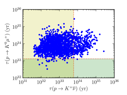
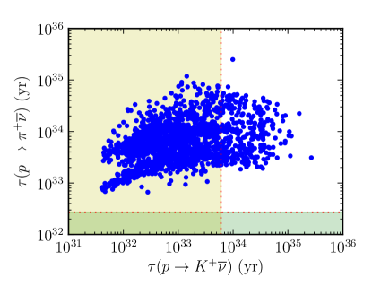
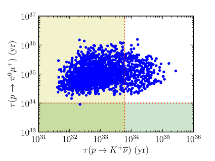
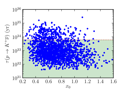
Figure 6: Comparisons of $K^{+}\bar{\nu}$ partial lifetime to those of other dominant modes in the model, and that lifetime as a function of the 10 mass parameter $x_{0}$, for the type-II case. Note the unsurprising preference for smaller $x_{0}$.

In order to locate an area of mixing parameter space which yields a sufficient $K^{+}\bar{\nu}$ lifetime, I wrote a supplementary Mathematica code to search for minima among strongly abridged versions of $\lvert\,\mathrm{C}_{\widetilde{W}}^{I}+\mathrm{C}_{\widetilde{W}}^{I\!V}\,\rvert$ and $\lvert\,\mathrm{C}_{\tilde{h}^{\pm}}^{I\!V}\,\rvert$ that contribute to the decay width. Specifically I started with $x_{0}$ terms only, corresponding to the baseline case, and then iteratively added back the largest contributions one by one while readjusting the initial values each time. Once all of the most important terms were present, I took the resulting mixing parameters as my initial values in the Python code. The resulting minimization gave a large percentage of trials with all six modes exceeding the lifetime bounds.

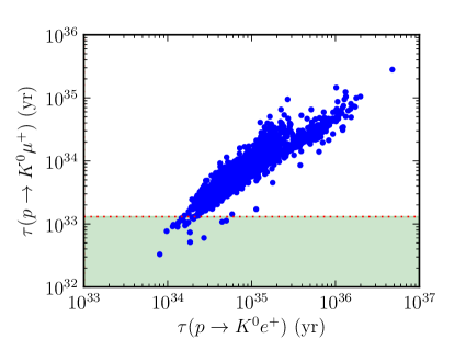
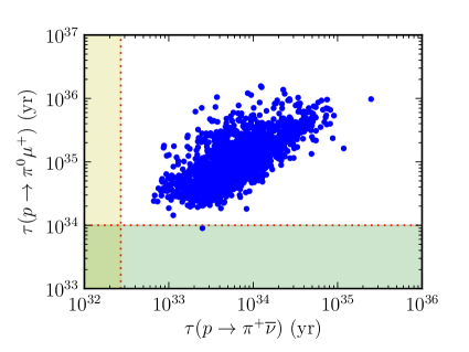
Figure 7: Comparisons of partial lifetimes among highly-correlated sub-dominant modes in the model for the type-II case.

With an allowed region of parameter space found, I expanded my searches to include a wider range of values for $x_{0}$. Using six different “seeds” for parameter values, all of which give every mode sufficient with $\tau(K^{+}\bar{\nu})$ roughly twice the experimental bound, I created a large number of trials for which the initial values were distributed normally around the seed values and with large standard deviations. The resulting data for such a search is shown in scatter plots below. Figure 6 gives the relationships between the $K^{+}\bar{\nu}$ mode and other representative modes and also the distribution of $K^{+}\bar{\nu}$ lifetime for varying $x_{0}$. Figure 7 shows the relationships between other more closely correlated modes for completeness.

Note the strong correlation between $\pi^{+}\bar{\nu}$ and $\pi^{0}\mu^{+}$, which are related by isospin, and the extreme correlation between $K^{0}e^{+}$ and $K^{0}\mu^{+}$. The latter is due to a manifestation of the hierarchical nature of the Yukawas in the $C_{ijkl}$, as well as minor features such $f_{11}\sim f_{12}$; similar structure is present in the $y^{f}$ and $U^{f}$, which tend to also have $11\sim 12$ or $11\ll 12$; these properties result in a straightforward scaling under the replacement $l:1\rightarrow 2$. Furthermore, the same relationship is present between $\pi^{0}e^{+}$ and $\pi^{0}\mu^{+}$. These relationships imply that the remaining plots I omitted differ only trivially from the representatives present.

I also performed simple scans in search of a maximum value for $\tau(K^{+}\bar{\nu})$, as well as taking note of any especially large values in the previous searches. While there does not seem to be any analytically-enforced maximum present in the model, I did consistently find that $\tau>10^{35}$ years was extremely rare, and I never saw a value higher than $\sim 6\!\times\!10^{35}$ yr. Given those findings, combined with the apparent smallness of the swath of parameter space yielding the above results and the low likelihood of a more global minimum based on my search methods, I believe that $\tau(K^{+}\bar{\nu})\mathrel{\vbox{\hbox{$>$}\nointerlineskip\hbox{$\sim$}}}10^{36}$ yr is statistically infeasible in this model for type-II seesaw. If such a value does exist, it is likely contained in a vanishingly small area of allowed parameter space and accomplished through truly extreme tuning. Therefore I will take $10^{36}$ years as a de facto upper limit on $\tau(K^{+}\bar{\nu})$ for the type-II case, which will not be accessible by Hyper-K and similar experiments hyperk ; dune in the near future, but should nonetheless allow the model to be tested eventually.

The other modes of course have similar limits, but it would seem that all the others are substantially higher and thus either far beyond the reach of the forthcoming experiments or beyond the contributions from gauge boson exchange, if not both, with the possible exception of $\tau(\pi^{+}\bar{\nu})$, which is rather highly correlated with $K^{+}\bar{\nu}$ in this model. Determining that value is tricky though because if I simply maximize the $\pi^{+}\bar{\nu}$ mode, then the $K^{+}\bar{\nu}$ mode will be below its bound; thus, there is some question as to how one defines the maximization.

Proton Partial Lifetimes for Type I Seesaw

I begin again by examining the same baseline case for the partial lifetimes, with $x_{0}\sim 1$ and all other $x_{i},y_{i}=0$. The resulting values for the dominant modes in the type-I case are given in Table 7. Here we see a much more favorable situation, in that even the $K^{+}\bar{\nu}$ mode decay width is sufficient, and in fact the other modes exceed the bounds by 2-4 orders of magnitude. Hence we expect that virtually all solutions will be adequate for modes other than $K^{+}\bar{\nu}$, and as long as there is no enhancement due to (de)tuning among the ${\rm C}^{\cal A}$ factors, that mode will be adequate as well.

This is of course a remarkable improvement over traditional models, yet it seems to contradict our expectations given then properties of the fermion fit. Why then is the model successful? There are two primary reasons, both of which are quite subtle. The first reason is that the smaller values for $g_{13}$ and $g_{23}$ seen in eq. (81) do in fact improve the situation, as I suggested, while the larger $f_{12}$ and $g_{12}$ seem to have less impact. Since $M\;(h_{33})$ is such an extremely dominant factor in the Yukawas, it is generally the case that contributions involving third generation are larger and more important than the others.

decay mode	baseline for $\tau$ (yrs)
$p\rightarrow K^{+}\bar{\nu}$	$7.87\!\times\!10^{33}$
$p\rightarrow K^{0}e^{+}$	$5.93\!\times\!10^{35}$
$p\rightarrow K^{0}\mu^{+}$	$2.45\!\times\!10^{35}$
$p\rightarrow\pi^{+}\bar{\nu}$	$2.37\!\times\!10^{36}$
$p\rightarrow\pi^{0}e^{+}$	$6.11\!\times\!10^{38}$
$p\rightarrow\pi^{0}\mu^{+}$	$2.27\!\times\!10^{38}$

Table 7: Hypothetical baseline partial lifetimes determined using type-I solution Yukawas and $x_{0}=0.95$ with all other $x_{i},y_{i}=0$. Note in comparing with Table 5 that all modes satisfy the lower limits, and most do so by several orders of magnitude.

The second reason is even more unexpected, to the point that it was not even examined in the preceding works on this ansatz. The unitary matrices $U^{f}$ for the charged fermions are generally $\sim 1$, just as one would expect, given the texture of CKM. This model is no exception, with off-diagonal terms generally ${\cal O}(10^{-1\mbox{-}3})$; however, with such sparse or hierarchical (flavor basis) Yukawas due to the ansatz, these “small” off-diagonal elements lead to “small” rotations of $h,f,g$ resulting in relatively substantial chanes to the textures of $\hat{h},\hat{f},\hat{g}$. Especially noteworthy are the changes in $h\rightarrow\hat{h}$, where some previously-zero off-diagonal elements are replaced by the same ${\cal O}(10^{-1\mbox{-}3})$ values seen in the $U^{f}$.

In light of the surprising non-triviality of the basis rotations, if we compare $U^{u,d}$ for the type-I case:

$$U^{u}= \left(\begin{array}[]{ccc}0.994&-0.1085+0.0057i&0.00298+10^{-5}i\\ 0.1084+0.0057i&0.994&0.0047+10^{-5}i\\ -0.0035-10^{-5}i&-0.0044+10^{-5}i&0.99998\end{array}\right)$$ (85)

$$U^{d}= \left(\begin{array}[]{ccc}0.967&-0.1087+0.2309i&0.00175+0.001175i\\ 0.1086+0.2308i&0.966&0.03935+0.00690i\\ -0.0076-0.0072i&-0.0381+0.00613i&0.9992\end{array}\right),$$ (89)

to those for the type-II case:

$$U^{u}= \left(\begin{array}[]{ccc}0.972&0.2098-0.1044i&-10^{-5}-0.010i\\ -0.210-0.1043i&0.971&-0.00012-0.0414i\\ -0.0043-0.001i&-0.001-0.0423i&0.999\end{array}\right)$$ (93)

$$U^{d}= \left(\begin{array}[]{ccc}0.9998&0.00633-0.0095i&0.00765-0.01117i\\ -0.00708-0.0095i&0.9983&0.03386-0.04514i\\ -0.00785-0.01054i&-0.03401-0.04514i&0.9983\end{array}\right),$$ (97)

we see that the off-diagonal entries are the same size or smaller for the type-I case in every entry except $U^{d}_{12}$; furthermore, several of the elements involving the third generation are smaller by an order of magnitude. These differences may seem rather benign, but in fact each of these slightly suppressed values individually translates into a factor of 10 suppression in most of the dominant $C$s, which all tend to involve third generation elements. In some cases two or even three such suppressions may affect a single ${\rm C}^{\cal A}$ factor. The squaring of factors in the decay width then gives suppressions of generally 2-4 orders of magnitude in the lifetimes, which is precisely what one can see when comparing Tables 6 and 7.

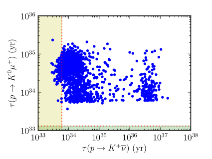
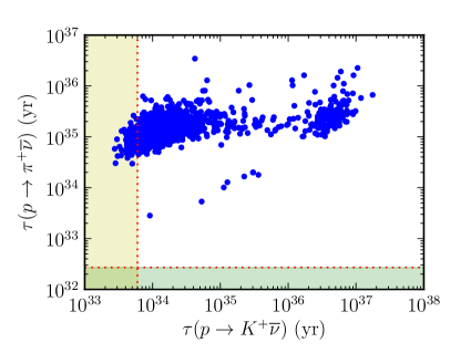
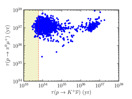
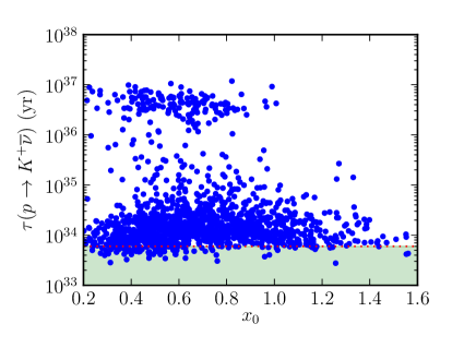
Figure 8: Comparisons of $K^{+}\bar{\nu}$ partial lifetime to those of other dominant modes in the model, and that lifetime as a function of the 10 mass parameter $x_{0}$, for the type-I case. Note the unsurprising preference for smaller $x_{0}$.

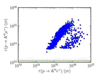
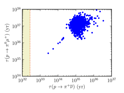
Figure 9: Comparisons of partial lifetimes among highly-correlated sub-dominant modes in the model for the type-I case.

Due to the more favorable circumstances, I was able to locate an allowed region of parameter space for type-I simply by running a large number of trials with the type-II parameter seeds. I repeated the process of expanding the range of $x_{0}$ by again choosing five seeds that gave every mode sufficient and $\tau(K^{+}\bar{\nu})$ roughly twice the experimental bound, and I again used those seeds to create scatter plots for a large number of trials. Figure 8 gives the relationships between the $K^{+}\bar{\nu}$ mode and other representative modes and the distribution of $\tau(K^{+}\bar{\nu})$ as a function of $x_{0}$, and Figure 9 shows the relationships between other more closely related modes. Note the bifurcation of the solution set in each plot; I have not yet been able to discover the cause of this behavior.

Again I performed scans to determine a statistical upper bound for the value of $\tau(K^{+}\bar{\nu})$ in the model. I consistently found that $\tau>10^{37}$ years was rare and did not see a value higher than $\sim 3\!\times\!10^{37}$ yr. Given those findings, I suspect that the de facto upper limit on $\tau(K^{+}\bar{\nu})$ for the type-II case is slightly lower than $10^{38}$ years for the type-I seesaw case. Such a value is clearly out of reach of Hyper-K and other imminent experiments. Note that as values for the neutral Kaon and pion lifetimes often exceeded $10^{38}$ years in my findings involving $K^{+}\bar{\nu}$ minimization, the upper limits for those modes are surely sub-dominant to gauge exchange as well as out of reach of experiments and so not of interest.

VI Conclusion

In this work I have presented a full analysis of the nature of proton decay in an $SO(10)$ model that has 10, $\overline{\bf{126}}$, and 120 Yukawa couplings with restricted textures intended to naturally give favorable results for proton lifetime as well as a realistic fermion sector. The model is capable of supporting either type-I or type-II dominance in the neutrino mass matrix, and I have analyzed both types throughout. Using, numerical minimization of chi-squares, I was able to obtain successful fits for all fermion sector parameters, including the $\theta_{13}$ reactor mixing angle, and for both seesaw types. Using the Yukawa couplings fixed by those fermion sector fits as input, I then searched the parameter space of the heavy triplet Higgs sector mixing for areas yielding adequate partial lifetimes, again using numerical minimization to optimize results. For the case with type-II seesaw, I found that lifetime limits for five of the six decay modes of interest are satisfied for nearly arbitrary values of the triplet mixing parameters, with an especially mild ${\cal O}(10^{-1})$ cancellation required in order to satisfy the limit for the $K^{+}\bar{\nu}$ mode. Additionally, I deduced that partial lifetime values of $\tau(K^{+}\bar{\nu})\mathrel{\vbox{\hbox{$>$}\nointerlineskip\hbox{$\sim$}}}10^{36}$ years are vanishingly unlikely in the model, implying the value can be taken as a de facto lifetime for the mode, which makes the model ultimately testable. For the case with type-I seesaw, I found that limits for all six decay modes of interest are satisfied for values of the triplet mixing parameters that do not result in substantial enhancement, with limits for modes other than $K^{+}\bar{\nu}$ satisfied for nearly arbitrary parameter values; furthermore, I deduced a statistical maximum lifetime for $K^{+}\bar{\nu}$ of just under $10^{38}$ years. Given these results, I conclude that the well-motivated Yukawa texture ansatz proposed by Dutta, Mimura, and Mohapatra is a phenomenological success, capable of suppressing proton decay without the usual need for cancellation and without compromising any aspect of the corresponding fermion mass spectrum.

Acknowledgements.

This work under Rabindra Mohapatra was supported by the University of Maryland, College Park Department of Physics and by National Science Foundation grant number PHY-1315155. I would like to thank R. Mohapatra for extensive discussion and guidance and Y. Mimura and B. Dutta for helpful correspondence. I would also like to thank M. Richman for assistance with numerical tools and programming.

Appendix A
Feynman Diagrams for All $d=6$ Operators Contributing to Proton Decay

Channels for $\boldsymbol{p\rightarrow\pi^{+}\bar{\nu}}$.

$i,l=1,2,3$; $\tilde{\phi}_{\cal T}$ is the Higgsino component of a heavy color-triplet Higgs superfield, $\phi={\rm H},\bar{\Delta},\Sigma$

Channels for $\boldsymbol{p\rightarrow\pi^{0}\ell^{+}}$.

$j=1,2,3$;  $l=1,2$ ($\leftrightarrow\ell=e,\mu$), or for diagrams including $l^{\prime}$, instead $l=1,2,3$ and $l^{\prime}=1,2$

Channels for $\boldsymbol{p\rightarrow K^{+}\bar{\nu}}$.

$i,l=1,2,3$; parentheses indicate coupled choices; the absence of a diagrams containing $\tilde{u}du\tilde{e}$ dressed by $\tilde{h}^{\pm}$ and $u\tilde{d}d\tilde{\nu}$ dressed by $\tilde{h}^{0}$ is due to resulting external $\nu^{\cal C}$

Channels for $\boldsymbol{p\rightarrow K^{0}\ell^{+}}$.

$j=1,2,3$;  $l=1,2$ ($\leftrightarrow\ell=e,\mu$), or for diagrams including $l^{\prime}$, instead $l=1,2,3$ and $l^{\prime}=1,2$

References

- (1) H. Fritzsch, P. Minkowski. Ann. Phys. 93 (1975) 93; H. Georgi, in Particles and Fields (ed. C. E. Carlson), A.I.P. (1975).
- (2) C. S. Aulakh, R. N. Mohapatra. Phys.Rev. D28 (1983) 217
- (3) T.E. Clark, Tzee-Ke Kuo, N. Nakagawa. Phys.Lett. B115 (1982) 26
- (4) K. S. Babu, R. N. Mohapatra. Phys. Rev. Lett. 70 (1993) 2845, [hep-ph/9209215].
- (5) K. S. Babu, C. Macesanu. Phys. Rev. D72, 115003 (2005) [hep-ph/0505200].
- (6) G. Lazarides, Q. Shafi, C. Wetterich. Nucl. Phys. B181 (1981) 287; J. Schechter, J. W. F. Valle. Phys. Rev. D22 (1980) 2227; R. N. Mohapatra, G. Senjanovic. Phys. Rev. D23 (1981) 165.
- (7) B. Bajc, G. Senjanovic, F. Vissani. hep-ph/0110310; Phys. Rev. Lett. 90, 051802 (2003) [hep-ph/0210207].
- (8) H. S. Goh, R. N. Mohapatra, S. P. Ng. Phys. Lett. B570 (2003) 215, [hep-ph/0303055]; Phys. Rev. D68, 115008 (2003) [hep-ph/0308197].
- (9) S. Bertolini, M. Frigerio, M. Malinsky. Phys. Rev. D70, 095002 (2004) [hep-ph/0406117]; S. Bertolini, T. Schwetz, M. Malinsky. Phys. Rev. D73, 115012 (2006) [hep-ph/0605006]; S. Bertolini, M. Malinsky, Phys. Rev. D72, 055021 (2005) [hep-ph/0504241]; A. S. Joshipura, K . M. Patel. arXiv:1105.5943 [hep-ph].
- (10) K. Matsuda, Y. Koide, T. Fukuyama. Phys. Rev. D64, 053015 (2001), [arXiv:hep-ph/0010026]; T. Fukuyama, N. Okada. JHEP 11 (2002) 011, [arXiv:hep-ph/0205066]; T. Fukuyama, A. Ilakovac, T. Kikuchi, S. Meljanac, N. Okada. JHEP 09 (2004) 052, [arXiv:hep-ph/0406068]; T. Fukuyama, A. Ilakovac, T. Kikuchi, S. Meljanac, N. Okada. Eur. Phys. J. C42 (2005) 191, [arXiv:hep-ph/0401213].
- (11) P. Minkowski. Phys. Lett. B67, 421 (1977); T. Yanagida in Workshop on Unified Theories, KEK Report 79-18 (1979) 95; M. Gell-Mann, P. Ramond, R. Slansky. Supergravity, 315, Amsterdam: North Holland (1979); S. L. Glashow. 1979 Cargese Summer Institute on Quarks and Leptons, 687, New York: Plenum (1980); R. N. Mohapatra, G. Senjanovic. Phys. Rev. Lett. 44 (1980) 912.
- (12) F. P. An et al. [DAYA-BAY Collaboration], Phys. Rev. Lett. 108, 171803 (2012) [arXiv:1203.1669 [hep-ex]]; J. K. Ahn et al. [RENO Collaboration], Phys. Rev. Lett. 108, 191802 (2012) [arXiv:1204.0626 [hep-ex]].
- (13) P. F. Harrison, D. H. Perkins, W. G. Scott. Phys.Lett. B458 (1999) 79, [hep-ph/9904297].
- (14) G. Altarelli, G. Blankenburg, JHEP 1103 (2011) 133, [arXiv:1012.2697 [hep-ph]].
- (15) P. S. Bhupal Dev, R. N. Mohapatra, M. Severson. Phys. Rev. D84, 053005 (2011), [arXiv:1107.2378 [hep-ph]].
- (16) P. S. Bhupal Dev, B. Dutta, R. N. Mohapatra, M. Severson. Phys. Rev. D86, 035002 (2012) [arXiv:1202.4012 [hep-ph]].
- (17) J. Gustafson et al. [Super-K Collaboration], Phys. Rev. D91, 072009 (2015), [arXiv:1504.01041 [hep-ex]].
- (18) B. Dutta, Y. Mimura, R. N. Mohapatra. Phys. Rev. D87, 075008 (2013), [arXiv:1302.2574 [hep-ph]].
- (19) B. Dutta, Y. Mimura, R. N. Mohapatra. Phys. Rev. D72, 075009 (2005), [arXiv:hep-ph/0507319].
- (20) B. Dutta, Y. Mimura, R. N. Mohapatra. JHEP 1005 (2010) 034, [arXiv:0911.2242 [hep-ph]].
- (21) C. S. Aulakh, S. K. Garg. Nucl. Phys. B857 (2012) 101, [arXiv:0807.0917 [hep-ph]].
- (22) V. M. Belyaev, M. I. Vysotsky. Phys. Lett. B127 (1983) 215.
- (23) H. S. Goh, R.N. Mohapatra, S. Nasri, Siew-Phang Ng. Phys. Lett. B587 (2004) 105, [arXiv:hep-ph/0311330].
- (24) K.A. Olive et al. (Particle Data Group), Chin. Phys. C, 38, 090001 (2014).
- (25) M. B. Gavela et al. Nucl. Phys. B312, 2 (1989) 269.
- (26) S. Aoki et al. Phys. Rev. D62, 014506 (2000), [arXiv:hep-lat/9911026].
- (27) M. Claudson, M. B. Wise, L. J. Hall. Nucl. Phys. B195 (1982) 297.
- (28) J. F. Donoghue, E. Golowich. Phys. Rev. D26 (1982) 3092.
- (29) M. Matsumoto, J. Arafune, H. Tanaka, K. Shiraishi. Phys. Rev. D46 (1992) 3966; J. Hisano, H. Murayama, T. Yanagida. Nucl. Phys. B402 (1993) 46.
- (30) F. James and M. Roos, Computer Physics Communications. 10 (1975) 343; http://seal.web.cern.ch/seal/MathLibs/5 10/Minuit2/html/
- (31) G. van Rossum and F.L. Drake (eds). Python Reference Manual, Virginia: Python Labs (2001); http://www.python.org
- (32) C.R. Das, M.K. Parida. Eur. Phys. Journal C20 (2001) 121 [arXiv:hep-ph/0010004].
- (33) K. Bora. Horizon, A Journal of Physics, 2 (2013) ISSN 2250-0871, [arXiv:1206.5909 [hep-ph]].
- (34) T. Blazek, S. Raby, S. Pokorski. Phys. Rev. D52, 4151 (1995) [hep-ph/9504364].
- (35) K. S. Babu et al. Report of the Community Summer Study (Snowmass 2013), Intensity Frontier – Baryon Number Violation Group, [arXiv:1311.5285 [hep-ph]].
- (36) K. Abe et al. [Hyper-K Collaboration], arXiv:1109.3262 [hep-ex].
- (37) C. Adams et al. [LBNF/DUNE Collaboration], arXiv:1307.7335 [hep-ex].