Running of Oscillation Parameters in Matter with Flavor-Diagonal Non-Standard Interactions of the Neutrino

Abstract

In this article we unravel the role of matter effect in neutrino oscillation in the presence of lepton-flavor-conserving, non-universal non-standard interactions (NSI’s) of the neutrino. Employing the Jacobi method, we derive approximate analytical expressions for the effective mass-squared differences and mixing angles in matter. It is shown that, within the effective mixing matrix, the Standard Model (SM) $W$-exchange interaction only affects $\theta_{12}$ and $\theta_{13}$, while the flavor-diagonal NSI’s only affect $\theta_{23}$. The CP-violating phase $\delta$ remains unaffected. Using our simple and compact analytical approximation, we study the impact of the flavor-diagonal NSI’s on the neutrino oscillation probabilities for various appearance and disappearance channels. At higher energies and longer baselines, it is found that the impact of the NSI’s can be significant in the $\nu_{\mu}\rightarrow\nu_{\mu}$ channel, which can probed in future atmospheric neutrino experiments, if the NSI’s are of the order of their current upper bounds. Our analysis also enables us to explore the possible degeneracy between the octant of $\theta_{23}$ and the sign of the NSI parameter for a given choice of mass hierarchy in a simple manner.

1 Introduction and Motivation

The recent measurement of the moderately large value of the 1-3 mixing angle An:2015rpe ; An:2013zwz ; An:2012bu ; Ahn:2012nd ; Abe:2011fz ; Abe:2012tg ; Abe:2013sxa ; Adamson:2013ue ; Abe:2013hdq ; Abe:2013xua ; Abe:2015awa , quite close to its previous upper limit Apollonio:1999ae ; Piepke:2002ju , strongly validates the standard three-flavor oscillation model of neutrinos Agashe:2014kda ; Hewett:2012ns , which has been quite successful in explaining all the neutrino oscillation data available so far Gonzalez-Garcia:2014bfa ; Capozzi:2013csa ; Forero:2014bxa , except for a few anomalies observed at very-short-baseline experiments Abazajian:2012ys . This fairly large value of $\theta_{13}$ greatly enhances the role of matter effects Wolfenstein:1977ue ; Mikheev:1986gs ; Mikheev:1986wj in currently running and upcoming long-baseline Agarwalla:2014fva ; Pascoli:2013wca ; Feldman:2013vca and atmospheric Wendell:2015ona ; Ahmed:2015jtv ; Devi:2014yaa ; Aartsen:2014oha neutrino oscillation experiments aimed at determining the remaining fundamental unknowns, in particular, the neutrino mass hierarchy, possible presence of a CP-violating phase $\delta$, and the octant ambiguity of $\theta_{23}$ Fogli:1996pv if the 2-3 mixing angle is non-maximal. A clear understanding of the sub-leading three-flavor effects Agarwalla:2013hma ; Minakata:2012ue in the neutrino oscillation probabilities in matter is mandatory to achieve the above goals.

Furthermore, in addition to the Standard Model (SM) $W$-exchange interaction, various models of physics beyond the SM predict non-standard interactions (NSI) of the neutrino Wolfenstein:1977ue ; Valle:1987gv ; Guzzo:1991hi ; Roulet:1991sm ; Grossman:1995wx , which could affect neutrino propagation through matter. Indeed, such NSI’s arise naturally in many neutrino-mass models Minkowski:1977sc ; Yanagida:1979as ; Mohapatra:1979ia ; GellMann:1980vs ; Schechter:1980gr ; Lazarides:1980nt ; Mohapatra:1986bd ; Akhmedov:1995ip ; Akhmedov:1995vm ; Dev:2009aw ; Boucenna:2014zba ; Cheng:1980qt ; Zee:1980ai ; Babu:1988ki ; Diaz:1997xc ; Hirsch:2000ef which attempt to explain the small neutrino masses and the relatively large neutrino mixing angles, as suggested by current oscillation data Gonzalez-Garcia:2014bfa ; Capozzi:2013csa ; Forero:2014bxa , as well as in many other models to be discussed in a later section. Thus, understanding how the presence of NSI’s would affect the three-flavor neutrino oscillation probabilities in matter is crucial in extracting the fundamental unknowns listed above, and also in searching for new-physics signatures in neutrino oscillation data.

While the three-flavor oscillation probabilities in matter can be calculated numerically on a computer, with or without NSI’s, and properly taking into account the changing mass-density along the baseline, the computer program is a blackbox which does not offer any deep understanding as to why the probabilities depend on the input parameters in a particular way. If the mass-density along the baseline is approximated by an average constant value, then exact analytical expressions for the three-flavor oscillation probabilities can, in principle, be derived as was done for the SM case in Refs. Barger:1980tf ; Zaglauer:1988gz ; Kimura:2002hb ; Kimura:2002wd . But even for the SM case, the expressions are extremely lengthy and too complicated to yield much physical insight. Thus, for the SM case, further approximations which simplify the analytic expressions while maintaining the essential physics have been developed by various authors Petcov:1986qg ; Kim:1986vg ; Arafune:1996bt ; Arafune:1997hd ; Ohlsson:1999xb ; Freund:2001pn ; Cervera:2000kp ; Akhmedov:2004ny ; Honda:2006hp ; Asano:2011nj ; Agarwalla:2013tza ; Minakata:2015gra to help us in this direction. Indeed, approximate analytical expressions of the SM neutrino oscillation probabilities in constant-density matter have played important roles in understanding the nature of the flavor transitions as functions of baseline $L$ and/or neutrino energy $E$ Freund:2001pn ; Cervera:2000kp ; Akhmedov:2004ny ; Asano:2011nj . To obtain similar insights for the NSI case, approximate analytical expressions for the three-flavor oscillation probabilities in constant-density matter in the presence of NSI’s are called for. Once they have provided us with the intuition we seek, on how and why the oscillation probabilities behave in a particular way, we can then resort to numerical techniques to further refine the analysis, e.g. taking into account the non-constant mass-density, if the need arises.

In previous works Agarwalla:2013tza ; Honda:2006hp , we looked at the matter effect on neutrino oscillation due to the SM $W$-exchange interaction between the matter electrons and the propagating electron neutrinos. Employing the Jacobi method Jacobi:1846 , we showed that the said matter effects could be absorbed into the ‘running’ of the effective mass-squared-differences, and the effective mixing angles $\theta_{12}$ and $\theta_{13}$ in matter as functions of the parameter $a=2\sqrt{2}G_{F}N_{e}E$, while the effective values of $\theta_{23}$ and the CP-violating phase $\delta$ remained unaffected. Here, $G_{F}$ is the Fermi muon decay constant, $N_{e}$ is the electron density, and $E$ is the energy of the neutrino. The approximate neutrino oscillation probabilities were obtained by simply replacing the oscillation parameters in the vacuum expressions for the probabilities with their running in-matter counterparts.

This running-effective-parameter approach has several advantages over other approaches which approximate the neutrino oscillation probabilities directly. First, the resulting expressions for the probabilities are strictly positive, which is not always the case when the probabilities are directly expanded in some small parameter, and the series truncated after a few terms. Second, the behavior of the oscillation probabilities as functions of $L$ and $E$ can be understood easily as due to the running of the oscillation parameters with $a$, as was shown in several examples in Refs. Agarwalla:2013tza ; Honda:2006hp . Third, as will be shown later, it is very convenient in exploring possible correlations and degeneracies among the mass-mixing parameters that may appear in matter in a non-trivial fashion.

In this paper, we extend our previous analysis and investigate how our conclusions are modified in the presence of neutrino NSI’s of the form

$$\mathcal{L}_{\mathrm{NC-NSI}}\;=\;-\sum_{\alpha\beta f}2\sqrt{2}G_{F}\varepsilon_{\alpha\beta}^{fC}\bigl{(}\overline{\nu_{\alpha}}\gamma^{\mu}P_{L}\nu_{\beta}\bigr{)}\bigl{(}\overline{f}\gamma_{\mu}P_{C}f\bigr{)}\;,$$ (1)

where subscripts $\alpha,\beta=e,\mu,\tau$ label the neutrino flavor, $f=e,u,d$ mark the matter fermions, $C=L,R$ denotes the chirality of the $ff$ current, and $\varepsilon_{\alpha\beta}^{fC}$ are dimensionless quantities which parametrize the strengths of the interactions. The hermiticity of the interaction demands

$$\varepsilon_{\beta\alpha}^{fC}\;=\;(\varepsilon_{\alpha\beta}^{fC})^{*}\;.$$ (2)

For neutrino propagation through matter, the relevant combinations are

$$\varepsilon_{\alpha\beta}\;\equiv\;\sum_{f=e,u,d}\varepsilon_{\alpha\beta}^{f}\dfrac{N_{f}}{N_{e}}\;\equiv\;\sum_{f=e,u,d}\left(\varepsilon_{\alpha\beta}^{fL}+\varepsilon_{\alpha\beta}^{fR}\right)\dfrac{N_{f}}{N_{e}}\;,$$ (3)

where $N_{f}$ denotes the density of fermion $f$. In this current work, we limit our investigation to flavor-diagonal NSI’s, that is, we only allow the $\varepsilon_{\alpha\beta}$’s with $\alpha=\beta$ to be non-zero. The case of flavor non-diagonal NSI’s will be considered in a separate work AgarwallaKaoSunTakeuchi:2015 .

In the following, we will show how the presence of such flavor-diagonal NSI’s affect the running of the effective neutrino oscillation parameters (the mass-squared differences, mixing angles, and CP-violating phase), and ultimately how they alter the oscillation probabilities. We find that due to the expected smallness of the $\varepsilon_{\alpha\alpha}$’s as compared to the SM $W$-exchange interaction, there is a clear separation in the ranges of $a$ at which the NSI’s and the SM interaction are respectively relevant. Furthermore, within the effective neutrino mixing matrix, the SM interaction only affects the running of $\theta_{12}$ and $\theta_{13}$, while the flavor-diagonal NSI’s only affect the running of $\theta_{23}$. The CP-violating phase $\delta$ remains unaffected and maintains its vacuum value.

We note that similar studies have been performed in the past by many authors e.g. in Refs. GonzalezGarcia:2001mp ; Ota:2001pw ; Yasuda:2007jp ; Kopp:2007ne ; Ribeiro:2007ud ; Blennow:2008eb ; Kikuchi:2008vq ; Meloni:2009ia ; Asano:2011nj . This work differs from these existing works in the use of the Jacobi method Jacobi:1846 to derive compact analytical formulae for the running effective mass-squared differences and effective mixing angles, which provide a clear and simple picture of how neutrino NSI’s affect neutrino oscillation. We also note that we have addressed the same problem with a similar approach previously in Refs. Honda:2006gv ; Honda:2006di ; Honda:2007yd ; Honda:2007wv . The current paper updates these works by allowing for a non-maximal value of $\theta_{23}$, a generic value of the CP-violating phase $\delta$, a larger range of $a$, and refinements on how the matter effect is absorbed into the running parameters.

This paper is organized as follows. We start section 2 with a discussion on neutrino NSI’s: how and where they arise, how they affect the propagation of the neutrinos in matter, and show that the linear combinations relevant for neutrino oscillation are $\eta=(\varepsilon_{\mu\mu}-\varepsilon_{\tau\tau})/2$ and $\zeta=\varepsilon_{ee}-(\varepsilon_{\mu\mu}+\varepsilon_{\tau\tau})/2$. This is followed by a brief discussion on the theoretical expectation for the sizes of these parameters, and their current experimental bounds. In section 3, we use the Jacobi method to calculate how the NSI parameter $\eta$ affects the running of the effective mass-squared differences, effective mixing angles, and the effective CP-violating phase as functions of $\hat{a}=a(1+\zeta)$ for the neutrinos. To check the accuracy of our method, we also present a comparison between our approximate analytical probability expressions and exact numerical calculations (for constant matter density) towards the end of this section. Section 4 describes the advantages of our analytical probability expressions to figure out the suitable testbeds to probe these NSI’s of the neutrino. In this section, we also present simple and compact analytical expressions exposing the possible correlations and degeneracies between $\theta_{23}$ and the NSI parameter $\eta$ under such situations. Finally, we summarize and draw our conclusions in section 5. The derivation of the running oscillation parameters for the anti-neutrino case is relegated to appendix A where we also compare our analytical results with exact numerical probabilities. In appendix B, we examine the differences in the exact numerical probabilities with line-averaged constant Earth density and varying Earth density profile for 8770 km and 10000 km baselines.

2 A Brief Tour of Non-Standard Interactions of the Neutrino

In this section, we first briefly discuss the various categories of models that give rise to NSI’s of neutrino.

2.1 Models that Predict NSI’s of the Neutrino

NSI’s of the neutrino arise in a variety of beyond the Standard Model (BSM) scenarios Honda:2006gv ; Honda:2006di ; Honda:2007yd ; Honda:2007wv ; Antusch:2008tz ; Ohlsson:2012kf via the direct tree-level exchange of new particles, or via flavor distinguishing radiative corrections to the $Z\nu\nu$ vertex Loinaz:1998jg ; Lebedev:1999vc ; Chang:2000xy , or indirectly via the non-unitarity of the lepton mixing matrix Antusch:2006vwa . BSM models which predict neutrino NSI’s include:

1. Models with a generation distinguishing $Z^{\prime}$ boson. This class includes gauged $L_{e}-L_{\mu}$ and gauged $L_{e}-L_{\tau}$ He:1990pn ; He:1991qd , gauged $B-\alpha L_{e}-\beta L_{\mu}-\gamma L_{\tau}$ (with $\alpha+\beta+\gamma=3$) Ma:1997nq ; Ma:1998dp ; Ma:1998dr ; Ma:1998zg ; Ma:1998xd ; Chang:2000xy , and topcolor assisted technicolor Hill:1994hp ; Loinaz:1998jg .

2. Models with leptoquarks Buchmuller:1986iq ; Buchmuller:1986zs ; Leurer:1993em ; Davidson:1993qk ; Hewett:1997ce and/or bileptons Cuypers:1996ia . These can be either scalar or vector particles. This class includes various Grand Unification Theory (GUT) models and extended technicolor (ETC) Dimopoulos:1979es ; Eichten:1979ah ; Dimopoulos:1980fj .

3. The Supersymmetric Standard Model with $R$-parity violation Barger:1989rk ; Dreiner:1997uz ; Barbier:2004ez ; Lebedev:1999vc ; Lebedev:1999ze . The super-partners of the SM particles play the role of the leptoquarks and bileptons of class 2.

4. Extended Higgs models. This class includes the Zee model Zee:1980ai , the Zee-Babu model Zee:1985id ; Babu:1988ki ; Ohlsson:2009vk , and various models with $SU(2)$ singlet Chikashige:1980ui ; Schechter:1981cv ; Fukugita:1988qe ; Bilenky:1993bt ; Antusch:2008tz and $SU(2)$ triplet Higgses Gelmini:1980re ; Schechter:1981cv ; Malinsky:2008qn , as well as the generation distinguishing $Z^{\prime}$ models listed under class 1.

5. Models with non-unitary neutrino mixing matrices Langacker:1988up ; Bilenky:1992wv ; Nardi:1994iv ; Tommasini:1995ii ; Bergmann:1998rg ; Czakon:2001em ; Fornengo:2001pm ; Bekman:2002zk ; Loinaz:2002ep ; Loinaz:2003gc ; Loinaz:2004qc ; Barger:2004db ; Antusch:2006vwa ; Malinsky:2009df ; Malinsky:2009gw ; Abazajian:2012ys ; Escrihuela:2015wra . Apparent non-unitarity of the mixing matrix for the three light neutrino flavors would result when it is part of a larger mixing matrix involving heavier and/or sterile fields.

Systematic studies of how NSI’s can arise in these, and other BSM theories can be found, for instance, in Refs. Honda:2007wv ; Antusch:2008tz ; Gavela:2008ra ; Ohlsson:2012kf . Thus, the ability to detect NSI’s in neutrino experiments would complement the direct searches for new particles at the LHC for a variety of BSM models. Next, we focus our attention to see the role of lepton-flavor-conserving NSI’s when neutrinos travel through the matter.

2.2 Lepton-Flavor-Conserving NSI’s

The NSI’s of Eq. (3) modify the effective Hamiltonian for neutrino propagation in matter in the flavor basis to

$$H\;=\;\dfrac{1}{2E}\left(U\begin{bmatrix}m_{1}^{2}&0&0\\ 0&m_{2}^{2}&0\\ 0&0&m_{3}^{2}\end{bmatrix}U^{\dagger}+a\begin{bmatrix}1+\varepsilon_{ee}&\varepsilon_{e\mu}&\varepsilon_{e\tau}\\ \varepsilon_{e\mu}^{*}&\varepsilon_{\mu\mu}&\varepsilon_{\mu\tau}\\ \varepsilon_{e\tau}^{*}&\varepsilon_{\mu\tau}^{*}&\varepsilon_{\tau\tau}\end{bmatrix}\right)$$ (4)

where $U$ is the vacuum Pontecorvo-Maki-Nakagawa-Sakata (PMNS) matrix Pontecorvo:1957vz ; Maki:1962mu ; Pontecorvo:1967fh , $E$ is the neutrino energy, the matter-effect parameter $a$ is given by

$$a\;=\;2\sqrt{2}G_{F}N_{e}E\;=\;7.6324\times 10^{-5}(\mathrm{eV}^{2})\left(\dfrac{\rho}{\mathrm{g/cm^{3}}}\right)\left(\dfrac{E}{\mathrm{GeV}}\right)\;.$$ (5)

For Earth matter, we can assume $N_{n}\approx N_{p}=N_{e}$, in which case $N_{u}\approx N_{d}\approx 3N_{e}$. Therefore,

$$\varepsilon_{\alpha\beta}\;=\;\varepsilon_{\alpha\beta}^{\oplus}\;\approx\;\varepsilon_{\alpha\beta}^{e}+3\,\varepsilon_{\alpha\beta}^{u}+3\,\varepsilon_{\alpha\beta}^{d}\;.$$ (6)

Since we restrict our attention to lepton-flavor-conserving NSI’s in this paper, the effective Hamiltonian in the flavor basis takes the form

$$H\;=\;\dfrac{1}{2E}\left(U\begin{bmatrix}m_{1}^{2}&0&0\\ 0&m_{2}^{2}&0\\ 0&0&m_{3}^{2}\end{bmatrix}U^{\dagger}+a\begin{bmatrix}1+\varepsilon_{ee}&0&0\\ 0&\varepsilon_{\mu\mu}&0\\ 0&0&\varepsilon_{\tau\tau}\end{bmatrix}\right)\;.$$ (7)

In the absence of off-diagonal terms, we can rewrite the matter effect matrix as follows:

$$\begin{bmatrix}1+\varepsilon_{ee}&0&0\\ 0&\varepsilon_{\mu\mu}&0\\ 0&0&\varepsilon_{\tau\tau}\end{bmatrix}$$ (8)

$$= \begin{bmatrix}1+\varepsilon_{ee}-\dfrac{\varepsilon_{\mu\mu}+\varepsilon_{\tau\tau}}{2}&0&0\\ 0&\left(\dfrac{\varepsilon_{\mu\mu}-\varepsilon_{\tau\tau}}{2}\right)&0\\ 0&0&-\left(\dfrac{\varepsilon_{\mu\mu}-\varepsilon_{\tau\tau}}{2}\right)\end{bmatrix}+\left(\dfrac{\varepsilon_{\mu\mu}+\varepsilon_{\tau\tau}}{2}\right)\begin{bmatrix}1&0&0\\ 0&1&0\\ 0&0&1\end{bmatrix}$$ (9)

$$= a\left(1+\varepsilon_{ee}-\dfrac{\varepsilon_{\mu\mu}+\varepsilon_{\tau\tau}}{2}\right)\begin{bmatrix}1&0&0\\ 0&\left(\dfrac{\varepsilon_{\mu\mu}-\varepsilon_{\tau\tau}}{2}\right)&0\\ 0&0&-\left(\dfrac{\varepsilon_{\mu\mu}-\varepsilon_{\tau\tau}}{2}\right)\end{bmatrix}$$ (11)

$$+\mbox{ $O(\varepsilon^{2})$ terms }+\mbox{ unit matrix term }\;,$$

where we have assumed that the $\varepsilon$’s are small compared to 1. Let

$$\eta\;\equiv\;\dfrac{\varepsilon_{\mu\mu}-\varepsilon_{\tau\tau}}{2}\;,\qquad\zeta\;\equiv\;\varepsilon_{ee}-\dfrac{\varepsilon_{\mu\mu}+\varepsilon_{\tau\tau}}{2}\;,$$ (12)

and

$$\hat{a}\;\equiv\;a(1+\zeta)\;.$$ (13)

Note that the NSI parameter $\eta$ introduced here is related to the parameter $\xi$ which was used in Ref. Honda:2006gv by

$$\eta\;=\;-\dfrac{\xi}{2}\;.$$ (14)

Thus, the effective Hamiltonian can be taken to be

$$H\;=\;\dfrac{1}{2E}\left(U\begin{bmatrix}m_{1}^{2}&0&0\\ 0&m_{2}^{2}&0\\ 0&0&m_{3}^{2}\end{bmatrix}U^{\dagger}+\hat{a}\begin{bmatrix}1&0&0\\ 0&\eta&0\\ 0&0&-\eta\end{bmatrix}\right)\;.$$ (15)

Note that the $\eta=0$ case simply replaces $a$ with $\hat{a}=a(1+\zeta)$ in the SM Hamiltonian. Thus, the effective mass-squared differences, mixing angles, and CP-violating phase have the same functional dependence on $\hat{a}$ as they had on $a$ in the SM case. In other words, a non-zero $\zeta$ simply rescales the value of $a$ by a constant factor. The presence of a non-zero $\eta$, on the other hand, requires us to diagonalize $H$ with a different unitary matrix from the $\eta=0$ case, and this will introduce corrections to the effective oscillation parameters beyond a simple rescaling of $a$. Next, we discuss the constraints that we have at present on these NSI parameters.

2.3 Existing Bounds on the NSI parameters

Before looking at the matter effect due to the neutrino NSI’s, let us first look at what is currently known about the sizes of the $\varepsilon_{\alpha\beta}^{fC}$’s and the combinations $\eta=(\varepsilon_{\mu\mu}-\varepsilon_{\tau\tau})/2$ and $\zeta=\varepsilon_{ee}-(\varepsilon_{\mu\mu}+\varepsilon_{\tau\tau})/2$.

2.3.1 Theoretical Expectation

Theoretically, the sizes of the NSI’s are generically expected to be small since they are putatively due to BSM physics at a much higher scale than the electroweak scale, or to loop effects. If they arise from the tree level exchange of new particles of mass $\Lambda$, which would be described by dimension six operators, we can expect the $\varepsilon_{\alpha\beta}^{fC}$’s to be of order $O(M_{W}^{2}/\Lambda^{2})$. Loop effects involving a heavy particle of mass $\Lambda$ would be further suppressed by a factor of $O(1/4\pi)$ or more. Processes that lead to dimension eight operators would be of order $O(M_{W}^{4}/\Lambda^{4})$. Thus, if we assume $\Lambda=O(1\,\mathrm{TeV})$, we expect the $\varepsilon_{\alpha\beta}^{fC}$’s, and consequently $\eta$ and $\zeta$, to be $O(10^{-3})$ or smaller.

2.3.2 Direct Experimental Bounds

Direct experimental bounds on the flavor-diagonal NSI parameters $\varepsilon_{\alpha\alpha}^{fC}$’s are available from a variety of sources. These include $\nu_{e}e$ scattering data from LAMPF Allen:1992qe and LSND Auerbach:2001wg , $\overline{\nu_{e}}e$ scattering data from the reactor experiments Irvine Reines:1976pv , Krasnoyarsk Vidyakin:1992nf , Rovno Derbin:1993wy , MUNU Daraktchieva:2003dr , and Texono Deniz:2009mu , $\nu_{e}q$ scattering data from CHARM Dorenbosch:1986tb , $\nu_{\mu}e$ scattering data from CHARM II Vilain:1993xb ; Vilain:1994qy , $\nu_{\mu}q$ scattering data from NuTeV Zeller:2001hh ; Ball:2009mk ; Bentz:2009yy , $e^{+}e^{-}\rightarrow\nu\overline{\nu}\gamma$ data from the LEP experiments ALEPH Barate:1997ue ; Barate:1998ci ; Heister:2002ut , L3 Acciarri:1997dq ; Acciarri:1998hb ; Acciarri:1999kp OPAL Ackerstaff:1996sd ; Ackerstaff:1997ze ; Abbiendi:1998yu ; Abbiendi:2000hh , and DELPHI Abdallah:2003np , and neutrino oscillation data from Super-Kamiokande Mitsuka:2011ty , IceCube and DeepCore Gross:2013iq ; Collaboration:2011ym , KamLAND Abe:2008aa , SNO Aharmim:2008kc , and Borexino Arpesella:2008mt ; Bellini:2011rx . These have been analyzed by various authors in Refs. Berezhiani:2001rs ; Berezhiani:2001rt ; Hirsch:2002uv ; Davidson:2003ha ; Maltoni:2002kq ; Friedland:2004pp ; Friedland:2004ah ; Friedland:2005vy ; Barranco:2005ps ; Barranco:2007ej ; Bolanos:2008km ; Escrihuela:2009up ; Biggio:2009kv ; Biggio:2009nt ; Forero:2011zz ; Escrihuela:2011cf ; Agarwalla:2012wf ; Esmaili:2013fva ; Khan:2013hva ; Khan:2014zwa ; Girardi:2014gna ; Girardi:2014kca ; Agarwalla:2014bsa , and collecting the results of the most recent analyses, we place the following 90% C.L. bounds on the flavor-diagonal vectorial NSI couplings:

$$\begin{array}[]{lll}|\varepsilon_{ee}^{e}|\;<\;0.1\;,&|\varepsilon_{ee}^{u}|\;<\;1\;,&|\varepsilon_{ee}^{d}|\;<\;1\;,\\ |\varepsilon_{\mu\mu}^{e}|\;<\;0.04\;,&|\varepsilon_{\mu\mu}^{u}|\;<\;0.04\;,&|\varepsilon_{\mu\mu}^{d}|\;<\;0.04\;,\\ |\varepsilon_{\tau\tau}^{e}|\;<\;0.6\;,&|\varepsilon_{\tau\tau}^{u}|\;<\;0.05\;,&|\varepsilon_{\tau\tau}^{d}|\;<\;0.05\;.\end{array}$$ (16)

Note that the current experimental bounds on the NSI couplings $\varepsilon_{\alpha\beta}^{fC}$ are weak compared to the theoretical expectation of $O(10^{-3})$, the 90% C.L. upper bound on their absolute values ranging from $O(10^{-2})$ to $O(1)$. To combine these bounds into bounds on the $\varepsilon_{\alpha\beta}$’s, we follow the procedure of Ref. Biggio:2009nt ,

$$|\varepsilon_{\alpha\beta}|\;\lesssim\;\sqrt{|\varepsilon_{\alpha\beta}^{e}|^{2}+|3\varepsilon_{\alpha\beta}^{u}|^{2}+|3\varepsilon_{\alpha\beta}^{d}|^{2}}\;,$$ (17)

and find

$$|\varepsilon_{ee}|\;<\;4\;,\qquad|\varepsilon_{\mu\mu}|\;<\;0.2\;,\qquad|\varepsilon_{\tau\tau}|\;<\;0.6\;.$$ (18)

Neglecting possible correlations among these parameters, these bounds can again be combined to yield

$$|\eta| < \sqrt{\dfrac{1}{4}|\varepsilon_{\mu\mu}|^{2}+\dfrac{1}{4}|\varepsilon_{\tau\tau}|^{2}}\;=\;0.3\;,$$ (19)

$$|\zeta| < \sqrt{|\varepsilon_{ee}|^{2}+\dfrac{1}{4}|\varepsilon_{\mu\mu}|^{2}+\dfrac{1}{4}|\varepsilon_{\tau\tau}|^{2}}\;=\;4\;.$$ (20)

A tighter bound exists for $\eta$ which has been obtained directly using solar and atmospheric neutrino data in Ref. Maltoni:2002kq , and more recently in Ref. GonzalezGarcia:2011my using atmospheric and MINOS data. In Ref. Maltoni:2002kq , only NSI’s with the $d$-quarks were considered and the following $3\sigma$ (99.7% C.L.) bounds were obtained:

$$-0.03\;<\;\varepsilon^{d}_{\mu\tau} < 0.02\;,$$ (21)

$$|\varepsilon^{d}_{\tau\tau}-\varepsilon^{d}_{\mu\mu}| < 0.05\;.$$ (22)

Since $N_{d}=N_{u}=3N_{e}$, Ref. Maltoni:2002kq is actually constraining $\varepsilon_{\alpha\beta}/3$, so this result can be interpreted as

$$-0.09\;<\;\varepsilon_{\mu\tau} < 0.06\;,$$ (23)

$$|\varepsilon_{\mu\mu}-\varepsilon_{\tau\tau}| < 0.15\;.$$ (24)

Rescaling to $1.64\sigma$ (90% C.L.), we find

$$|\eta|\;=\;\left|\dfrac{\varepsilon_{\mu\mu}-\varepsilon_{\tau\tau}}{2}\right|\;<\;0.04\;.$$ (25)

Ref. GonzalezGarcia:2011my gives slightly different 90% C.L. bounds of

$$|\varepsilon_{\mu\tau}| < 0.035\;,$$ (26)

$$|\varepsilon_{\mu\mu}-\varepsilon_{\tau\tau}| < 0.11\;,$$ (27)

which translates to

$$|\eta|\;=\;\left|\dfrac{\varepsilon_{\mu\mu}-\varepsilon_{\tau\tau}}{2}\right|\;<\;0.055\;.$$ (28)

Thus, though $\eta$ and $\zeta$ are expected theoretically to be $O(10^{-3})$, their current 90% C.L. experimental bounds are respectively $\sim\!0.05$ and $O(1)$.

3 Effective Mixing Angles and Effective Mass-Squared Differences
– Neutrino Case

3.1 Setup of the Problem

Parameter	Best-fit Value & 1$\sigma$ Range	Benchmark Value
$\quad\delta m^{2}_{21}\quad$	$\quad(7.50\pm 0.185)\times 10^{-5}\ {\rm eV}^{2}\quad$	$\quad 7.50\times 10^{-5}\ {\rm eV}^{2}\quad$
$\delta m^{2}_{31}$	$(2.47^{+0.069}_{-0.067})\times 10^{-3}\ {\rm eV}^{2}$	$2.47\times 10^{-3}\ {\rm eV}^{2}$
$\sin^{2}\theta_{23}$	$0.41^{+0.037}_{-0.025}\oplus 0.59^{+0.021}_{-0.022}$	$0.41$
$\theta_{23}/^{\circ}$	$40.0^{+2.1}_{-1.5}\oplus 50.4^{+1.2}_{-1.3}$
$\theta_{23}/\mathrm{rad}$	$0.698^{+0.037}_{-0.026}\oplus 0.880^{+0.021}_{-0.023}$
$\sin^{2}\theta_{12}$	$0.30\pm 0.013$	$0.30$
$\theta_{12}/^{\circ}$	$33.3\pm 0.8$
$\theta_{12}/\mathrm{rad}$	$0.580\pm 0.014$
$\sin^{2}\theta_{13}$	$0.023\pm 0.0023$	$0.023$
$\theta_{13}/^{\circ}$	$8.6^{+0.44}_{-0.46}$
$\theta_{13}/\mathrm{rad}$	$0.15\pm 0.01$
$\delta/^{\circ}$	$300^{+66}_{-138}$	$0$
$\delta/\pi$	$1.67^{+0.37}_{-0.77}$

Table 1: Second column shows the best-fit values and 1$\sigma$ uncertainties on the oscillation parameters taken from Ref. GonzalezGarcia:2012sz . We use the values listed in the third column as benchmark values for which we calculate our oscillation probabilities in this work.

As we have seen, in the presence of non-zero $\eta$ and $\zeta$, the effective Hamiltonian (times $2E$) for neutrino propagation in Earth matter is given by

$$H_{\eta}\;=\;\overset{\lower 1.0pt\hbox{$\scriptstyle{\sim}$}}{U}\begin{bmatrix}\lambda_{1}&0&0\\ 0&\lambda_{2}&0\\ 0&0&\lambda_{3}\end{bmatrix}\overset{\lower 1.0pt\hbox{$\scriptstyle{\sim}$}}{U}^{\dagger}\;=\;\underbrace{U\begin{bmatrix}0&0&0\\ 0&\delta m_{21}^{2}&0\\ 0&0&\delta m_{31}^{2}\end{bmatrix}U^{\dagger}+\hat{a}\underbrace{\begin{bmatrix}1&0&0\\ 0&0&0\\ 0&0&0\end{bmatrix}}_{\displaystyle\equiv M_{a}}}_{\displaystyle\equiv H_{0}}+\hat{a}\eta\underbrace{\begin{bmatrix}0&0&0\\ 0&1&0\\ 0&0&-1\end{bmatrix}}_{\displaystyle\equiv M_{\eta}}\;,$$ (29)

where $\hat{a}=a(1+\zeta)$. The problem is to diagonalize $H_{\eta}=H_{0}+\hat{a}\eta M_{\eta}$ and find the eigenvalues $\lambda_{i}$ ($i=1,2,3$) and the diagonalization matrix $\overset{\lower 1.0pt\hbox{$\scriptstyle{\sim}$}}{U}$ as functions of $\hat{a}$ and $\eta$.

To this end, we utilize the method used in Refs. Agarwalla:2013tza ; Honda:2006hp where approximate expressions for the $\lambda_{i}$’s and $\overset{\lower 1.0pt\hbox{$\scriptstyle{\sim}$}}{U}$ were derived for $H_{0}$, the $\eta=0$ case, using the Jacobi method Jacobi:1846 . The Jacobi method entails diagonalizing $2\times 2$ submatrices of a matrix in the order which requires the the largest rotation angles until the off-diagonal elements are negligibly small. In the case of $H_{0}$, it was discovered in Refs. Agarwalla:2013tza ; Honda:2006hp that two $2\times 2$ rotations were sufficient to render it approximately diagonal, and that these two rotation angles could be absorbed into ‘running’ values of $\theta_{12}$ and $\theta_{13}$. The procedure that we use in the following for $H_{\eta}$ is to add on the $\hat{a}\eta M_{\eta}$ term to $H_{0}$ after it is approximately diagonalized, and then proceed with a third $2\times 2$ rotation to rotate away the additional off-diagonal terms.

As the order parameter to evaluate the sizes of the off-diagonal elements, we use

$$\epsilon\;\equiv\;\sqrt{\dfrac{\delta m^{2}_{21}}{|\delta m^{2}_{31}|}}\;\approx\;0.17\;,$$ (30)

and consider $H_{0}$ and $H_{\eta}$ to be approximately diagonalized when the rotation angles required for further diagonalization are of order $\epsilon^{3}=0.005$ or smaller. Note that we are using a slightly different epsilon ($\epsilon$) here to distinguish this quantity from the NSI’s ($\varepsilon_{\alpha\beta}$).

The eigenvalues $\lambda_{i}$ ($i=1,2,3$) and the diagonalization matrix $\overset{\lower 1.0pt\hbox{$\scriptstyle{\sim}$}}{U}$ of $H_{\eta}$ are necessarily functions of $\hat{a}=2\sqrt{2}G_{F}N_{e}E(1+\zeta)$. In order to parametrize the size of $\hat{a}$, we find it convenient to introduce the log-scale variable Agarwalla:2013tza ; Honda:2006hp

$$\beta\equiv-\log_{\epsilon}\dfrac{\hat{a}}{|\delta m^{2}_{31}|}\;,$$ (31)

so that $\hat{a}=\delta m^{2}_{21}$ corresponds to $\beta=-2$, and $\hat{a}=|\delta m^{2}_{31}|$ corresponds to $\beta=0$. In the following, various quantities will be plotted as functions of $\beta$.

Unless otherwise stated, we use the benchmark values of the various oscillation parameters as given in the third column of Table 1 to draw our plots. These values are taken from Ref. GonzalezGarcia:2012sz and correspond to the case in which reactor fluxes have been left free in the fit and short-baseline reactor data with $L\leq 100$ m are included. For $\sin^{2}\theta_{23}$, we consider the benchmark value which lies in the lower octant and CP-violating phase $\delta$ is assumed to be zero. These choices of the oscillation parameters are well within their 3$\sigma$ allowed ranges which are obtained in recent global fit analyses Forero:2014bxa ; Capozzi:2013csa ; Gonzalez-Garcia:2014bfa . We also present results considering other allowed values of $\sin^{2}\theta_{23}$ and $\delta$ which we discuss in section 3.5. In the evaluation of the sizes of the elements of the effective Hamiltonian, we will assume $\theta_{13}\approx 0.15=O(\epsilon)$, $\cos(2\theta_{12})/2\approx 0.2=O(\epsilon)$, and $|\cos(2\theta_{23})|\approx 0.18=O(\epsilon)$. We also assume that the NSI parameter $\eta$ is of order $\epsilon^{2}=0.03$ (or smaller), since the current 90% C.L. ($1.64\sigma$) upper bound on $|\eta|$ was $\sim 0.05$, cf. Eqs. (25) and (28), though we allow it to be as large as $0.1$ in our plots to enhance and make visible the effect of a non-zero $\eta$.

3.2 Diagonalization of the Effective Hamiltonian

3.2.1 Change to the Mass Eigenbasis in Vacuum

Introducing the matrix

$$Q_{3}=\mathrm{diag}(1,1,e^{i\delta})\;,$$ (32)

we begin by partially diagonalizing the Hamiltonian $H_{\eta}$ as

$$H_{\eta}^{\prime} = Q_{3}^{\dagger}U^{\dagger}H_{\eta}UQ_{3}$$ (33)

$$= \underbrace{\left[\begin{array}[]{ccc}0&0&0\\ 0&\delta m^{2}_{21}&0\\ 0&0&\delta m^{2}_{31}\end{array}\right]+\hat{a}\underbrace{Q_{3}^{\dagger}U^{\dagger}\underbrace{\left[\begin{array}[]{ccc}1&0&0\\ 0&0&0\\ 0&0&0\end{array}\right]}_{\displaystyle M_{a}}UQ_{3}}_{\displaystyle\equiv M^{\prime}_{a}(\theta_{12},\theta_{13},\theta_{23})}}_{\displaystyle\equiv H_{0}^{\prime}}+\hat{a}\eta\,\underbrace{Q_{3}^{\dagger}U^{\dagger}\underbrace{\left[\begin{array}[]{ccc}0&0&0\\ 0&1&0\\ 0&0&-1\end{array}\right]}_{\displaystyle M_{\eta}}UQ_{3}}_{\displaystyle\equiv M^{\prime}_{\eta}(\theta_{12},\theta_{13},\theta_{23},\delta)}\;,$$ (43)

where

$$M^{\prime}_{a}(\theta_{12},\theta_{13},\theta_{23})\;=\;Q_{3}^{\dagger}\left[\begin{array}[]{ccc}U^{*}_{e1}U_{e1}&U^{*}_{e1}U_{e2}&U^{*}_{e1}U_{e3}\\ U^{*}_{e2}U_{e1}&U^{*}_{e2}U_{e2}&U^{*}_{e2}U_{e3}\\ U^{*}_{e3}U_{e1}&U^{*}_{e3}U_{e2}&U^{*}_{e3}U_{e3}\end{array}\right]Q_{3}\;=\;\left[\begin{array}[]{ccc}c_{12}^{2}c_{13}^{2}&c_{12}s_{12}c_{13}^{2}&c_{12}c_{13}s_{13}\\ c_{12}s_{12}c_{13}^{2}&s_{12}^{2}c_{13}^{2}&s_{12}c_{13}s_{13}\\ c_{12}c_{13}s_{13}&s_{12}c_{13}s_{13}&s_{13}^{2}\end{array}\right]\;,$$ (44)

and

$$M^{\prime}_{\eta}(\theta_{12},\theta_{13},\theta_{23},\delta)$$ (45)

$$= Q_{3}^{\dagger}\left\{\left[\begin{array}[]{ccc}U^{*}_{\mu 1}U_{\mu 1}&U^{*}_{\mu 1}U_{\mu 2}&U^{*}_{\mu 1}U_{\mu 3}\\ U^{*}_{\mu 2}U_{\mu 1}&U^{*}_{\mu 2}U_{\mu 2}&U^{*}_{\mu 2}U_{\mu 3}\\ U^{*}_{\mu 3}U_{\mu 1}&U^{*}_{\mu 3}U_{\mu 2}&U^{*}_{\mu 3}U_{\mu 3}\end{array}\right]-\left[\begin{array}[]{ccc}U^{*}_{\tau 1}U_{\tau 1}&U^{*}_{\tau 1}U_{\tau 2}&U^{*}_{\tau 1}U_{\tau 3}\\ U^{*}_{\tau 2}U_{\tau 1}&U^{*}_{\tau 2}U_{\tau 2}&U^{*}_{\tau 2}U_{\tau 3}\\ U^{*}_{\tau 3}U_{\tau 1}&U^{*}_{\tau 3}U_{\tau 2}&U^{*}_{\tau 3}U_{\tau 3}\end{array}\right]\right\}Q_{3}$$ (52)

$$= \left[\begin{array}[]{l}\sin(2\theta_{12})\sin(2\theta_{23})s_{13}\cos\delta+(s_{12}^{2}-c_{12}^{2}s_{13}^{2})\cos(2\theta_{23})\\ (s_{12}^{2}e^{-i\delta}-c_{12}^{2}e^{i\delta})s_{13}\sin(2\theta_{23})-(1+s_{13}^{2})s_{12}c_{12}\cos(2\theta_{23})\\ -s_{12}c_{13}\sin(2\theta_{23})e^{-i\delta}+c_{12}s_{13}c_{13}\cos(2\theta_{23})\end{array}\right.$$ (64)

$$\qquad\qquad\begin{array}[]{l}(s_{12}^{2}e^{i\delta}-c_{12}^{2}e^{-i\delta})s_{13}\sin(2\theta_{23})-(1+s_{13}^{2})s_{12}c_{12}\cos(2\theta_{23})\\ -\sin(2\theta_{12})\sin(2\theta_{23})s_{13}\cos\delta+(c_{12}^{2}-s_{12}^{2}s_{13}^{2})\cos(2\theta_{23})\\ \phantom{-}c_{12}c_{13}\sin(2\theta_{23})e^{-i\delta}+s_{12}s_{13}c_{13}\cos(2\theta_{23})\end{array}$$

$$\qquad\qquad\qquad\qquad\left.\begin{array}[]{l}-s_{12}c_{13}\sin(2\theta_{23})e^{+i\delta}+c_{12}s_{13}c_{13}\cos(2\theta_{23})\\ \phantom{-}c_{12}c_{13}\sin(2\theta_{23})e^{+i\delta}+s_{12}s_{13}c_{13}\cos(2\theta_{23})\\ -c_{13}^{2}\cos(2\theta_{23})\end{array}\right]\;.$$

Using $\cos(2\theta_{23})=O(\epsilon)$ and $\theta_{13}=O(\epsilon)$, we estimate the sizes of the elements of $M_{a}$ to be:

$$M_{a}\;=\;\left[\begin{array}[]{ccc}O(1)&O(1)&O(\epsilon)\\ O(1)&O(1)&O(\epsilon)\\ O(\epsilon)&O(\epsilon)&O(\epsilon^{2})\end{array}\right]\;,$$ (65)

and those of $M_{\eta}$ to be

$$M_{\eta}\;=\;\left[\begin{array}[]{ccc}O(\epsilon)&O(\epsilon)&O(1)\\ O(\epsilon)&O(\epsilon)&O(1)\\ O(1)&O(1)&O(\epsilon)\end{array}\right]\;.$$ (66)

Given that we have assumed $\eta=O(\epsilon^{2})$ or smaller, the off-diagonal elements of $\eta M_{\eta}$ are suppressed compared to those of $M_{a}$, and only become important for $\hat{a}\gtrsim|\delta m^{2}_{31}|$, or equivalently, $\beta\gtrsim 0$.

3.2.2 Diagonalization of a $2\times 2$ hermitian matrix

The Jacobi method entails diagonalizing $2\times 2$ submatrices repeatedly. For this, it is convenient to note that given a $2\times 2$ hermitian matrix,

$$\begin{bmatrix}A&B\,e^{iD}\\ B\,e^{-iD}&C\end{bmatrix}\;=\;\begin{bmatrix}1&0\\ 0&e^{-iD}\end{bmatrix}\begin{bmatrix}A&B\\ B&C\end{bmatrix}\begin{bmatrix}1&0\\ 0&e^{iD}\end{bmatrix}\;,\qquad A,B,C,D\in\mathbb{R}\;,$$ (67)

the unitary matrix which diagonalizes this is given by

$$U\;=\;\begin{bmatrix}c_{\omega}&s_{\omega}e^{iD}\\ -s_{\omega}e^{-iD}&c_{\omega}\end{bmatrix}\;=\;\begin{bmatrix}1&0\\ 0&e^{-iD}\end{bmatrix}\begin{bmatrix}c_{\omega}&s_{\omega}\\ -s_{\omega}&c_{\omega}\end{bmatrix}\begin{bmatrix}1&0\\ 0&e^{iD}\end{bmatrix}\;,$$ (68)

where

$$c_{\omega}\;=\;\cos\omega\;,\qquad s_{\omega}\;=\;\sin\omega\;,\qquad\tan 2\omega\;=\;\dfrac{2B}{C-A}\;.$$ (69)

That is,

$$U^{\dagger}\begin{bmatrix}A&B\,e^{iD}\\ B\,e^{-iD}&C\end{bmatrix}U\;=\;\begin{bmatrix}\Lambda_{1}&0\\ 0&\Lambda_{2}\end{bmatrix}\;,$$ (70)

where

$$\Lambda_{1} = \dfrac{Ac^{2}_{\omega}-Cs^{2}_{\omega}}{c^{2}_{\omega}-s^{2}_{\omega}}\;=\;\dfrac{(A+C)\mp\sqrt{(A-C)^{2}+4B^{2}}}{2}\;,$$ (71)

$$\Lambda_{2} = \dfrac{Cc^{2}_{\omega}-As^{2}_{\omega}}{c^{2}_{\omega}-s^{2}_{\omega}}\;=\;\dfrac{(A+C)\pm\sqrt{(A-C)^{2}+4B^{2}}}{2}\;,$$ (72)

the double signs corresponding to the two possible quadrants for $2\omega$ that satisfy Eq. (69). In applying the above formula to our problem, care needs to be taken to choose the correct quadrant and sign combination so that the resulting effective mixing angles and mass-squared eigenvalues run smoothly from their vacuum values.

3.2.3 $\eta=0$ Case, First and Second Rotations

As mentioned above, we will first approximately diagonalize $H^{\prime}_{0}$, and add on the $\hat{a}\eta M^{\prime}_{\eta}$ term afterwards. Here, we reproduce how the Jacobi method was applied to $H_{0}^{\prime}$ in Refs. Agarwalla:2013tza ; Honda:2006hp . There, a $(1,2)$ rotation was applied to $H_{0}^{\prime}$, followed by a $(2,3)$ rotation, which was sufficient to approximately diagonalize $H_{0}^{\prime}$.

1. First Rotation

   

   

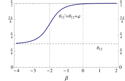
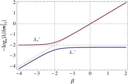
   Figure 1: (a) The dependence of $\theta^{\prime}_{12}$ on $\beta=-\log_{\,\epsilon}\left(\hat{a}/|\delta m^{2}_{31}|\right)$. (b) The $\beta$-dependence of $\lambda^{\prime}_{\pm}$.

   

   

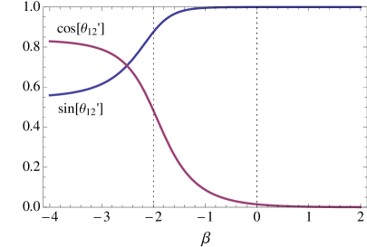
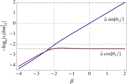
   Figure 2: (a) The dependence of $s^{\prime}_{12}=\sin\theta^{\prime}_{12}$ and $c^{\prime}_{12}=\cos\theta^{\prime}_{12}$ on $\beta=-\log_{\,\epsilon}\left(\hat{a}/|\delta m^{2}_{31}|\right)$. (b) The dependence of $\hat{a}s^{\prime}_{12}$ and $\hat{a}c^{\prime}_{12}$ on $\beta$. The values are given in units of $|\delta m^{2}_{31}|$. The asymptotic value of $\hat{a}c^{\prime}_{12}$ is $\delta m^{2}_{21}s_{12}c_{12}/c_{13}^{2}\approx 0.014\;|\delta m^{2}_{31}|=O(\varepsilon^{2}|\delta m^{2}_{31}|)$.

   Define the matrix $V$ as:

   $$V\;=\;\begin{bmatrix}c_{\varphi}&s_{\varphi}&0\\ -s_{\varphi}&c_{\varphi}&0\\ 0&0&1\end{bmatrix}\;,$$ (73)

   where

   $$c_{\varphi}\,=\,\cos\varphi\;,\quad s_{\varphi}\,=\,\sin\varphi\;,\quad\tan 2\varphi\,\equiv\,\dfrac{\hat{a}c_{13}^{2}\sin 2\theta_{12}}{\delta m^{2}_{21}-\hat{a}c_{13}^{2}\cos 2\theta_{12}}\;,\quad\left(0\leq\varphi<\frac{\pi}{2}-\theta_{12}\right)\;.$$ (74)

   Then,

   $$H_{0}^{\prime\prime}=V^{\dagger}H_{0}^{\prime}V=\left[\begin{array}[]{ccc}\lambda^{\prime}_{-}&0&\hat{a}c^{\prime}_{12}c_{13}s_{13}\\ 0&\lambda^{\prime}_{+}&\hat{a}s^{\prime}_{12}c_{13}s_{13}\\ \hat{a}c^{\prime}_{12}c_{13}s_{13}&\hat{a}s^{\prime}_{12}c_{13}s_{13}&\delta m^{2}_{31}+\hat{a}\,s_{13}^{2}\end{array}\right]\;,$$ (75)

   where

   $${c}_{12}^{\prime}=\cos\theta_{12}^{\prime}\;,\quad{s}_{12}^{\prime}=\sin\theta_{12}^{\prime}\;,\quad{\theta}_{12}^{\prime}=\theta_{12}+\varphi\;,$$ (76)

   and

   $$\lambda^{\prime}_{\pm}\;=\;\dfrac{(\hat{a}c_{13}^{2}+\delta m^{2}_{21})\pm\sqrt{(\hat{a}c_{13}^{2}-\delta m^{2}_{21})^{2}+4\hat{a}c_{13}^{2}s_{12}^{2}\delta m^{2}_{21}}}{2}\;.$$ (77)

   The angle $\theta_{12}^{\prime}=\theta_{12}+\varphi$ can be calculated directly without calculating $\varphi$ via

   $$\tan 2\theta^{\prime}_{12}\;=\;\dfrac{\delta m^{2}_{21}\sin 2\theta_{12}}{\delta m^{2}_{21}\cos 2\theta_{12}-\hat{a}c^{2}_{13}}\;,\qquad\left(\theta_{12}\leq\theta^{\prime}_{12}\leq\dfrac{\pi}{2}\right)\;.$$ (78)

   As $\beta$ is increased beyond $-2$, the $\lambda^{\prime}_{\pm}$ asymptote to

   $$\lambda^{\prime}_{+} \rightarrow \hat{a}c_{13}^{2}+\delta m^{2}_{21}s_{12}^{2}\;,$$ (79)

   $$\lambda^{\prime}_{-} \rightarrow \delta m^{2}_{21}c_{12}^{2}\;.$$ (80)

   The dependences of $\theta^{\prime}_{12}$ and $\lambda^{\prime}_{\pm}$ on $\beta$ are plotted in Fig. 1. Note that $\theta^{\prime}_{12}$ increases monotonically from $\theta_{12}$ to $\pi/2$ with increasing $\beta$. The $\beta$-dependence of $s^{\prime}_{12}=\sin\theta^{\prime}_{12}$ and $c^{\prime}_{12}=\cos\theta^{\prime}_{12}$ are shown in Fig. 2(a). As $\beta$ is increased beyond $-2$, that is $\hat{a}=\delta m^{2}_{21}$, $s^{\prime}_{12}$ grows rapidly to one while $c^{\prime}_{12}$ damps quickly to zero. In fact, the product $\hat{a}c^{\prime}_{12}$ stops increasing at around $\beta=-2$ and plateaus to the asymptotic value of $\delta m^{2}_{21}s_{12}c_{12}/c_{13}^{2}\approx 0.014\;|\delta m^{2}_{31}|=O(\varepsilon^{2})|\delta m^{2}_{31}|$ as shown in Fig. 2(b). That is:

   $$\hat{a}s_{12}^{\prime} = |\delta m^{2}_{31}|\,O(\epsilon^{-\beta})\;,$$ (81)

   $$\hat{a}c_{12}^{\prime} = |\delta m^{2}_{31}|\,O(\epsilon^{-\min(\beta,-2)})\;\leq\;|\delta m^{2}_{31}|\,O(\epsilon^{2})\;.$$ (82)

   Note also that the scales of $\lambda^{\prime}_{\pm}$ are given by

   $$\lambda^{\prime}_{+} = O(\max(\delta m^{2}_{21},\hat{a}))\;=\;|\delta m^{2}_{31}|\,O(\epsilon^{-\max(\beta,-2)})\;,$$ (83)

   $$\lambda^{\prime}_{-} = O(\min(\delta m^{2}_{21},\hat{a}))\;=\;|\delta m^{2}_{31}|\,O(\epsilon^{-\min(\beta,-2)})\;.$$ (84)

2. Second Rotation

   Given that the $(1,3)$ element of $H^{\prime\prime}_{0}$, namely $\hat{a}c^{\prime}_{12}c_{13}s_{13}$, is at most of order $|\delta m^{2}_{31}|O(\epsilon^{3})$ for all $\hat{a}$, whereas the $(2,3)$ element $\hat{a}s^{\prime}_{12}c_{13}s_{13}$ will continue to increase with $\hat{a}$, it is the $(2,3)$ submatrix that needs to be diagonalized next. The matrix $W$ which diagonalizes the $(2,3)$ submatrix of $H_{0}^{\prime\prime}$ is

   $$W=\begin{bmatrix}1&0&0\\ 0&c_{\phi}&s_{\phi}\\ 0&-s_{\phi}&c_{\phi}\end{bmatrix}\;,$$ (85)

   where $c_{\phi}=\cos\phi$, $s_{\phi}=\sin\phi$, and

   $$\tan 2\phi\;\equiv\;\dfrac{2\hat{a}s^{\prime}_{12}s_{13}c_{13}}{\delta m^{2}_{31}+\hat{a}s_{13}^{2}-\lambda^{\prime}_{+}}\;\approx\;\dfrac{\hat{a}\sin 2\theta_{13}}{(\delta m^{2}_{31}-\delta m^{2}_{21}s^{2}_{12})-\hat{a}\cos 2\theta_{13}}\;.$$ (86)

   The angle $\phi$ is in the first quadrant when $\delta m^{2}_{31}>0$ (normal hierarchy) and increases from zero to $\frac{\pi}{2}-\theta_{13}$ as $\beta$ is increased. $\phi$ is in the fourth quadrant when $\delta m^{2}_{31}<0$ (inverted hierarchy) and decreases from zero to $-\theta_{13}$ as $\beta$ is increased. This $\beta$-dependence of $\phi$ is shown in Fig. 3(a) for both mass hierarchies.

   

   

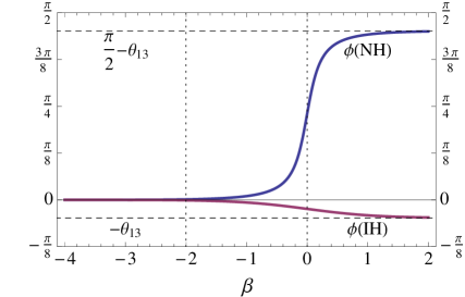
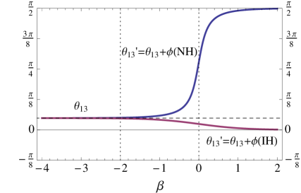
   Figure 3: The dependence of (a) $\phi$ and (b) $\theta^{\prime}_{13}=\theta_{13}+\phi$ on $\beta=-\log_{\,\epsilon}\left(\hat{a}/|\delta m^{2}_{31}|\right)$ for the normal (NH) and inverted (IH) mass hierarchies.

   

   (a) Normal Hierarchy

   

   (b) Inverted Hierarchy

   Figure 4: The $\beta$-dependence of $\lambda^{\prime\prime}_{\pm}$ for the (a) normal and (b) inverted mass hierarchies.

   Using $W$, we obtain

   $$H_{0}^{\prime\prime\prime} = W^{\dagger}H_{0}^{\prime\prime}W$$ (87)

   $$= \begin{bmatrix}\lambda^{\prime}_{-}&-\hat{a}{c}_{12}^{\prime}c_{13}s_{13}s_{\phi}&\hat{a}{c}_{12}^{\prime}c_{13}s_{13}c_{\phi}\\ -\hat{a}{c}_{12}^{\prime}c_{13}s_{13}s_{\phi}&\lambda^{\prime\prime}_{\mp}&0\\ \hat{a}{c}_{12}^{\prime}c_{13}s_{13}c_{\phi}&0&\lambda^{\prime\prime}_{\pm}\end{bmatrix}\;,$$ (88)

   where the upper signs are for the $\delta m^{2}_{31}>0$ (normal hierarchy) case and the lower signs are for the $\delta m^{2}_{31}<0$ (inverted hierarchy) case, with

   $$\lambda^{\prime\prime}_{\pm}\equiv\dfrac{[\lambda^{\prime}_{+}+(\delta m^{2}_{31}+\hat{a}s_{13}^{2})]\pm\sqrt{[\lambda^{\prime}_{+}-(\delta m^{2}_{31}+\hat{a}s_{13}^{2})]^{2}+4(\hat{a}s^{\prime}_{12}c_{13}s_{13})^{2}}}{2}\;.$$ (89)

   As $\beta$ is increased beyond 0, the $\lambda^{\prime\prime}_{\pm}$ asymptote to

   $$\lambda^{\prime\prime}_{+} \rightarrow \hat{a}+\delta m^{2}_{31}s_{13}^{2}+\delta m^{2}_{21}s_{12}^{2}c_{13}^{2}\;,$$ (90)

   $$\lambda^{\prime\prime}_{-} \rightarrow \delta m^{2}_{31}c_{13}^{2}+\delta m^{2}_{21}s_{12}^{2}s_{13}^{2}\;,$$ (91)

   for both mass hierarchies. Note that $\lambda^{\prime\prime}_{-}<0$ for the $\delta m^{2}_{31}<0$ case. The $\beta$-dependences of $\lambda^{\prime\prime}_{\pm}$ are shown in Fig. 4. Order-of-magnitude-wise, we have

   $$\begin{array}[]{lll}\lambda^{\prime\prime}_{-}\;=\;|\delta m^{2}_{31}|\,O(\epsilon^{-\max(\min(\beta,0),-2)})\;,&\phantom{|}\lambda^{\prime\prime}_{+}\phantom{|}\;=\;|\delta m^{2}_{31}|\,O(\epsilon^{-\max(\beta,0)})\;,&\mbox{if $\delta m^{2}_{31}>0$}\;,\\ \lambda^{\prime\prime}_{+}\;=\;|\delta m^{2}_{31}|\,O(\epsilon^{-\max(\beta,-2)})\;,&|\lambda^{\prime\prime}_{-}|\;=\;|\delta m^{2}_{31}|\,O(1)\;,&\mbox{if $\delta m^{2}_{31}<0$}\;.\end{array}$$ (92)

   In particular, in the range $\beta\gtrsim 0$ we have

   $$\begin{array}[]{lll}\lambda^{\prime\prime}_{-}\;=\;|\delta m^{2}_{31}|\,O(1)\;,&\phantom{|}\lambda^{\prime\prime}_{+}\phantom{|}\;=\;|\delta m^{2}_{31}|\,O(\epsilon^{-\beta})\;,&\mbox{if $\delta m^{2}_{31}>0$}\;,\\ \lambda^{\prime\prime}_{+}\;=\;|\delta m^{2}_{31}|\,O(\epsilon^{-\beta})\;,&|\lambda^{\prime\prime}_{-}|\;=\;|\delta m^{2}_{31}|\,O(1)\;,&\mbox{if $\delta m^{2}_{31}<0$}\;.\end{array}$$ (93)

   For the off-diagonal terms, since $\hat{a}c^{\prime}_{12}=|\delta m^{2}_{31}|O(\epsilon^{2})$, $c_{13}=O(1)$, $s_{13}=O(\epsilon)$, $s_{\phi}=O(1/\epsilon)$, $c_{\phi}=O(\epsilon/1)$, we have

   $$-\hat{a}c^{\prime}_{12}c_{13}s_{13}s_{\phi} = O(\epsilon^{3}/\epsilon^{4}),$$

   $$\hat{a}c^{\prime}_{12}c_{13}s_{13}c_{\phi} = O(\epsilon^{4}/\epsilon^{3}).$$ (94)

   Thus, looking at the sizes of the elements of $H^{\prime\prime\prime}_{0}$ in that range we find:

   $$H^{\prime\prime\prime}_{0}\;=\;|\delta m^{2}_{31}|\begin{bmatrix}O(\epsilon^{2})&O(\epsilon^{3}/\epsilon^{4})&O(\epsilon^{4}/\epsilon^{3})\\ O(\epsilon^{3}/\epsilon^{4})&O(1/\epsilon^{-\beta})&0\\ O(\epsilon^{4}/\epsilon^{3})&0&O(\epsilon^{-\beta}/1)\end{bmatrix}\;,$$ (95)

   where the elements with two entries denote the two different mass hierarchies, $O(\mathrm{NH}/\mathrm{IH})$, and we can see that further diagonalization only require angles of order $O(\epsilon^{3})$. Therefore, $H^{\prime\prime\prime}_{0}$ can be considered approximately diagonal.

3.2.4 $\eta\neq 0$ Case, Third Rotation

Let us now consider the $\eta\neq 0$ case. If we perform the same $(1,2)$ rotation $V$ on $H_{\eta}^{\prime}=H_{0}^{\prime}+\hat{a}\eta M^{\prime}_{\eta}$ as we did on $H_{0}^{\prime}$, the $M^{\prime}_{\eta}$ part is transformed to

$$V^{\dagger}M^{\prime}_{\eta}(\theta_{12},\theta_{13},\theta_{23},\delta)V = M^{\prime}_{\eta}(\underbrace{\theta_{12}+\varphi}_{\displaystyle=\theta^{\prime}_{12}},\theta_{13},\theta_{23},\delta)$$ (96)

$$= M^{\prime}_{\eta}(\theta^{\prime}_{12},\theta_{13},\theta_{23},\delta)\;.$$ (97)

Using $\theta^{\prime}_{12}\rightarrow\frac{\pi}{2}$, $\hat{a}s^{\prime}_{12}\rightarrow\hat{a}$, and $\hat{a}c^{\prime}_{12}\rightarrow O(\epsilon^{2})|\delta m^{2}_{31}|$ as $\beta$ is increased beyond $-2$, we can approximate

$$\hat{a}\eta M^{\prime}_{\eta}\left(\theta^{\prime}_{12},\theta_{13},\theta_{23},\delta\right)$$ (98)

$$\approx \hat{a}\eta M^{\prime}_{\eta}\left(\frac{\pi}{2},\theta_{13},\theta_{23},\delta\right)$$ (99)

$$= \hat{a}\eta\begin{bmatrix}\cos(2\theta_{23})&e^{i\delta}s_{13}\sin(2\theta_{23})&-e^{i\delta}c_{13}\sin(2\theta_{23})\\ e^{-i\delta}s_{13}\sin(2\theta_{23})&-s_{13}^{2}\cos(2\theta_{23})&s_{13}c_{13}\cos(2\theta_{23})\\ -e^{-i\delta}c_{13}\sin(2\theta_{23})&s_{13}c_{13}\cos(2\theta_{23})&-c_{13}^{2}\cos(2\theta_{23})\end{bmatrix}\;.$$ (100)

Performing the $(2,3)$ rotation $W$ next, we find:

$$W^{\dagger}M^{\prime}_{\eta}\left(\frac{\pi}{2},\theta_{13},\theta_{23},\delta\right)W$$ (101)

$$= M^{\prime}_{\eta}\Bigl{(}\frac{\pi}{2},\underbrace{\theta_{13}+\phi}_{\displaystyle=\theta^{\prime}_{13}},\theta_{23},\delta\Bigr{)}$$ (102)

$$= M^{\prime}_{\eta}\left(\frac{\pi}{2},\theta^{\prime}_{13},\theta_{23},\delta\right)$$ (103)

$$= \begin{bmatrix}\cos(2\theta_{23})&e^{i\delta}s_{13}^{\prime}\sin(2\theta_{23})&-e^{i\delta}c_{13}^{\prime}\sin(2\theta_{23})\\ e^{-i\delta}s_{13}^{\prime}\sin(2\theta_{23})&-s_{13}^{\prime 2}\cos(2\theta_{23})&s_{13}^{\prime}c_{13}^{\prime}\cos(2\theta_{23})\\ -e^{-i\delta}c_{13}^{\prime}\sin(2\theta_{23})&s_{13}^{\prime}c_{13}^{\prime}\cos(2\theta_{23})&-c_{13}^{\prime 2}\cos(2\theta_{23})\end{bmatrix}\;,$$ (104)

where $s^{\prime}_{13}=\sin\theta_{13}^{\prime}$ and $c^{\prime}_{13}=\cos\theta_{13}^{\prime}$. The angle $\theta^{\prime}_{13}=\theta_{13}+\phi$ can be calculated directly without the need to calculate $\phi$ using

$$\tan 2\theta^{\prime}_{13}\;=\;\dfrac{(\delta m^{2}_{31}-\delta m^{2}_{21}s_{12}^{2})\sin 2\theta_{13}}{(\delta m^{2}_{31}-\delta m^{2}_{21}s_{12}^{2})\cos 2\theta_{13}-\hat{a}}\;,$$ (105)

and its $\beta$-dependence is shown in Fig. 3(b). As can be seen, $\theta_{13}^{\prime}$ increases rapidly to $\pi/2$ when $\delta m^{2}_{31}>0$, while damping quickly to zero when $\delta m^{2}_{31}<0$, once $\beta$ is increased above zero. Consequently, $\hat{a}\cos\theta^{\prime}_{13}$ for the $\delta m^{2}_{31}>0$ case, and $\hat{a}\sin\theta^{\prime}_{13}$ for the $\delta m^{2}_{31}<0$ case plateau to $c_{13}s_{13}(1-\epsilon^{2}s_{12}^{2})|\delta m^{2}_{31}|=O(\epsilon)|\delta m^{2}_{31}|$ as $\beta$ is increased as shown in Fig. 5. Note that in the $\delta m^{2}_{31}>0$ case, $\hat{a}\cos\theta^{\prime}_{13}$ increases to $O(1)|\delta m^{2}_{31}|$ in the vicinity of $\beta=0$ before plateauing to $O(\epsilon)|\delta m^{2}_{31}|$. This will cause a slight problem in our approximation later. We now look at the normal and inverted mass hierarchy cases separately.

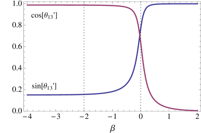
(a) Normal Hierarchy

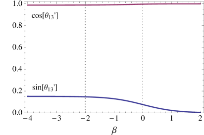
(b) Inverted Hierarchy

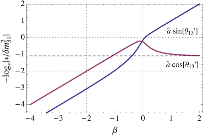
(c) Normal Hierarchy

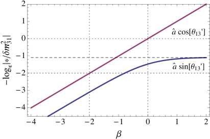
(d) Inverted Hierarchy

Figure 5: The dependence of $\sin\theta^{\prime}_{13}$ and $\cos\theta^{\prime}_{13}$ on $\beta=-\log_{\,\epsilon}\left(\hat{a}/|\delta m^{2}_{31}|\right)$ for the (a) normal and (b) inverted mass hierarchies. The dependence of $\hat{a}\sin\theta^{\prime}_{13}$ and $\hat{a}\cos\theta^{\prime}_{13}$ on $\beta=-\log_{\,\epsilon}\left(\hat{a}/|\delta m^{2}_{31}|\right)$ for the (c) normal and (d) inverted mass hierarchies.

1. $\bm{\delta m^{2}_{31}>0}$ Case

   For the $\delta m^{2}_{31}>0$ case $\hat{a}c^{\prime}_{13}\rightarrow O(\epsilon)|\delta m^{2}_{31}|$ as $\beta$ is increased beyond 0. Therefore, we can approximate

   $$H_{\eta}^{\prime\prime\prime} = W^{\dagger}V^{\dagger}H_{\eta}^{\prime}VW$$ (106)

   $$\approx H_{0}^{\prime\prime\prime}+\hat{a}\eta M^{\prime}_{\eta}\left(\frac{\pi}{2},\theta^{\prime}_{13},\theta_{23},\delta\right)$$ (107)

   $$\approx \begin{bmatrix}\lambda^{\prime}_{-}+\hat{a}\eta\cos(2\theta_{23})&\hat{a}\eta e^{i\delta}s_{13}^{\prime}\sin(2\theta_{23})&0\\ \hat{a}\eta e^{-i\delta}s_{13}^{\prime}\sin(2\theta_{23})&\lambda^{\prime\prime}_{-}-\hat{a}\eta s_{13}^{\prime 2}\cos(2\theta_{23})&0\\ 0&0&\lambda^{\prime\prime}_{+}\end{bmatrix}\;,$$ (108)

   where we have dropped off-diagonal terms of order $O(\epsilon^{3})|\delta m^{2}_{31}|$ or smaller. (This approximation breaks down in the vicinity of $\beta=0$ where both $\hat{a}s^{\prime}_{13}$ and $\hat{a}c^{\prime}_{13}$ are of order $O(1)|\delta m^{2}_{31}|$.) Define the matrix $X$ as

   $$X=\left[\begin{array}[]{ccc}c_{\chi}&s_{\chi}e^{i\delta}&0\\ -s_{\chi}e^{-i\delta}&c_{\chi}&0\\ 0&0&1\end{array}\right]\;,$$ (109)

   where $c_{\chi}=\cos\chi$, $s_{\chi}=\sin\chi$, and

   $$\quad\tan 2\chi \equiv \dfrac{2\hat{a}\eta s_{13}^{\prime}\sin(2\theta_{23})}{(\lambda^{\prime\prime}_{-}-\lambda^{\prime}_{-})-\hat{a}\eta(1+s_{13}^{\prime 2})\cos(2\theta_{23})}$$ (110)

   $$\approx \dfrac{2\hat{a}\eta\sin(2\theta_{23})}{[\delta m^{2}_{31}c_{13}^{2}-\delta m^{2}_{21}(c_{12}^{2}-s_{12}^{2}s_{13}^{2})]-2\hat{a}\eta\cos(2\theta_{23})}\;.$$ (111)

   Note that

   $$0\;\leq\;\chi\;<\;\dfrac{\pi}{2}-\theta_{23}\quad\mbox{for $\eta>0$,}\quad-\theta_{23}\;<\;\chi\;\leq\;0\quad\mbox{for $\eta<0$}\;.$$ (112)

   The $\beta$-dependence of $\chi$ is shown in Fig. 6 for several values of $\eta$, both positive (Fig. 6(a)) and negative (Fig. 6(b)).

   

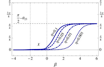
   (a) $\eta>0$

   

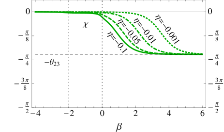
   (b) $\eta<0$

   

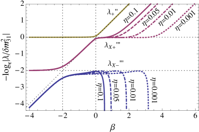
   (c) $\eta>0$

   

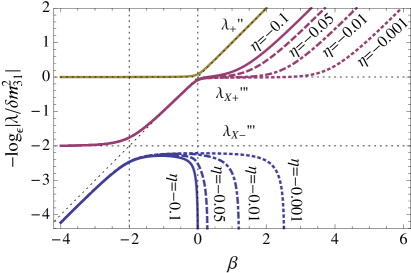
   (d) $\eta<0$

   

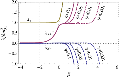
   (e) $\eta>0$

   

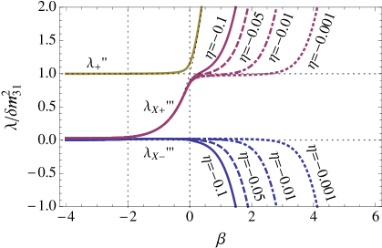
   (f) $\eta<0$

   Figure 6: The $\beta$-dependence of $\chi$ and $\lambda^{\prime\prime\prime}_{X\pm}$ for several values of $\eta$ with $s_{23}^{2}=0.4$.

   Using $X$, we find

   $$H^{\prime\prime\prime\prime}_{\eta+}\;=\;X^{\dagger}H^{\prime\prime\prime}_{\eta}X\;\approx\;\begin{bmatrix}\lambda^{\prime\prime\prime}_{X-}&0&0\\ 0&\lambda^{\prime\prime\prime}_{X+}&0\\ 0&0&\lambda^{\prime\prime}_{+}\end{bmatrix}\;,$$ (113)

   where

   $$\lambda^{\prime\prime\prime}_{X\pm}$$ (114)

   $$\equiv \dfrac{(\lambda^{\prime\prime}_{-}+\lambda^{\prime}_{-}+\hat{a}\eta c_{13}^{\prime 2}\cos 2\theta_{23})\pm\sqrt{[\lambda^{\prime\prime}_{-}-\lambda^{\prime}_{-}-\hat{a}\eta(1+s_{13}^{\prime 2})\cos 2\theta_{23}]^{2}+4(\hat{a}\eta s_{13}^{\prime}\sin 2\theta_{23})^{2}}}{2}\;.$$ (115)

   Thus, $H_{\eta+}^{\prime\prime\prime\prime}$ is approximately diagonal. The asymptotic forms of $\lambda_{X\pm}^{\prime\prime\prime}$ at $\beta\gg 0$ are

   $$\lambda^{\prime\prime\prime}_{X+} \rightarrow \phantom{-}\hat{a}|\eta|+\left\{\begin{array}[]{ll}\delta m^{2}_{31}c_{13}^{2}s_{23}^{2}+\delta m^{2}_{21}(c_{12}^{2}c_{23}^{2}+s_{12}^{2}s_{13}^{2}s_{23}^{2})&\mbox{for $\eta>0$}\\ \delta m^{2}_{31}c_{13}^{2}c_{23}^{2}+\delta m^{2}_{21}(c_{12}^{2}s_{23}^{2}+s_{12}^{2}s_{13}^{2}c_{23}^{2})&\mbox{for $\eta<0$}\end{array}\right.$$ (119)

   $$\lambda^{\prime\prime\prime}_{X-} \rightarrow -\hat{a}|\eta|+\left\{\begin{array}[]{ll}\delta m^{2}_{31}c_{13}^{2}c_{23}^{2}+\delta m^{2}_{21}(c_{12}^{2}s_{23}^{2}+s_{12}^{2}s_{13}^{2}c_{23}^{2})&\mbox{for $\eta>0$}\\ \delta m^{2}_{31}c_{13}^{2}s_{23}^{2}+\delta m^{2}_{21}(c_{12}^{2}c_{23}^{2}+s_{12}^{2}s_{13}^{2}s_{23}^{2})&\mbox{for $\eta<0$}\end{array}\right.$$ (122)

   The $\beta$-dependence of $\lambda^{\prime\prime\prime}_{X\pm}$ are shown in Figs. 6(c) to 6(f).

2. $\bm{\delta m^{2}_{31}<0}$ Case

   For the $\delta m^{2}_{31}<0$ case we have $\hat{a}s^{\prime}_{13}\rightarrow O(\epsilon)|\delta m^{2}_{31}|$ as $\beta$ is increased beyond 0. Therefore, we can approximate

   $$H_{\eta}^{\prime\prime\prime} = W^{\dagger}V^{\dagger}H_{\eta}^{\prime}VW$$ (123)

   $$\approx H_{0}^{\prime\prime\prime}+\hat{a}\eta M^{\prime}_{\eta}\left(\frac{\pi}{2},\theta^{\prime}_{13},\theta_{23},\delta\right)$$ (124)

   $$\approx \begin{bmatrix}\lambda^{\prime}_{-}+\hat{a}\eta\cos(2\theta_{23})&0&-\hat{a}\eta e^{i\delta}c^{\prime}_{13}\sin(2\theta_{23})\\ 0&\lambda^{\prime\prime}_{+}&0\\ -\hat{a}\eta e^{-i\delta}c_{13}^{\prime}\sin(2\theta_{23})&0&\lambda^{\prime\prime}_{-}-\hat{a}\eta c_{13}^{\prime 2}\cos(2\theta_{23})\end{bmatrix}\;,$$ (125)

   where we have dropped off-diagonal terms of order $O(\epsilon^{3})|\delta m^{2}_{31}|$ or smaller. Unlike the $\delta m^{2}_{31}>0$ case, this approximation is valid in the vicinity of $\beta=0$ since $\hat{a}s^{\prime}_{13}$ never exceeds $O(\epsilon)|\delta m^{2}_{31}|$ for all $\hat{a}$.

   Define the matrix $Y$ as

   $$Y\;=\;\left[\begin{array}[]{ccc}c_{\psi}&0&-s_{\psi}e^{i\delta}\\ 0&1&0\\ s_{\psi}e^{-i\delta}&0&c_{\psi}\end{array}\right]\;,$$ (126)

   where $c_{\psi}=\cos\psi$, $s_{\psi}=\sin\psi$, and

   $$\tan 2\psi \equiv \dfrac{2\hat{a}\eta c^{\prime}_{13}\sin(2\theta_{23})}{(\lambda^{\prime\prime}_{-}-\lambda^{\prime}_{-})-\hat{a}\eta(1+c_{13}^{\prime 2})\cos(2\theta_{23})}$$ (127)

   $$\approx -\dfrac{2\hat{a}\eta\sin(2\theta_{23})}{[|\delta m^{2}_{31}|c_{13}^{2}+\delta m^{2}_{21}(c_{12}^{2}-s_{12}^{2}s_{13}^{2})]+2\hat{a}\eta\cos(2\theta_{23})}\;.$$ (128)

   Note that

   $$-\theta_{23}\;<\;\psi\;\leq\;0\quad\mbox{for $\eta<0$}\;,\quad 0\;\leq\;\psi\;<\;\dfrac{\pi}{2}-\theta_{23}\quad\mbox{for $\eta>0$}\;.$$ (129)

   Comparing Eq. (111) and Eq. (128), we can infer that $\psi(\eta)\approx\chi(-\eta)$, the small difference due to the $\delta m^{2}_{21}$ term in the denominator of the expressions for $\tan 2\chi$ and $\tan 2\psi$. This can be seen in Fig. 7 where the $\beta$-dependence of $\psi$ is shown for several values of $\eta$, both positive (Fig. 7(a)) and negative (Fig. 7(b)).

   

   (a) $\eta>0$

   

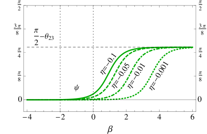
   (b) $\eta<0$

   

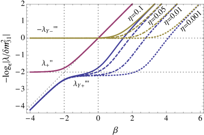
   (c) $\eta>0$

   

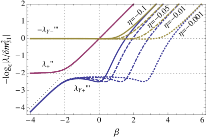
   (d) $\eta<0$

   

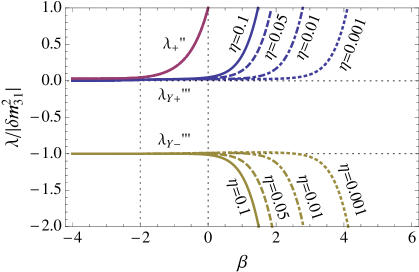
   (e) $\eta>0$

   

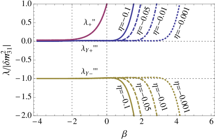
   (f) $\eta<0$

   Figure 7: The $\beta$-dependence of $\psi$ and $\lambda^{\prime\prime\prime}_{Y\pm}$ for several values of $\eta$ with $s_{23}^{2}=0.4$.

   Using $Y$, we find

   $$H^{\prime\prime\prime\prime}_{\eta-}\;=\;Y^{\dagger}H^{\prime\prime\prime}Y\;\approx\;\left[\begin{array}[]{ccc}\lambda^{\prime\prime\prime}_{Y+}&0&0\\ 0&\lambda^{\prime\prime}_{+}&0\\ 0&0&\lambda^{\prime\prime\prime}_{Y-}\end{array}\right]\;,$$ (130)

   where,

   $$\lambda^{\prime\prime\prime}_{Y\pm}$$ (131)

   $$\equiv \dfrac{(\lambda^{\prime\prime}_{-}+\lambda^{\prime}_{-}+\hat{a}\eta s_{13}^{\prime 2}\cos 2\theta_{23})\pm\sqrt{[\lambda^{\prime\prime}_{-}-\lambda^{\prime}_{-}-\hat{a}\eta(1+c_{13}^{\prime 2})\cos 2\theta_{23}]^{2}+4(\hat{a}\eta c_{13}^{\prime}\sin 2\theta_{23})^{2}}}{2}\;.$$ (132)

   Thus, $H_{\eta-}^{\prime\prime\prime\prime}$ is approximately diagonal. The asymptotic forms of $\lambda^{\prime\prime\prime}_{Y\pm}$ at $\beta\gg 0$ are

   $$\lambda^{\prime\prime\prime}_{Y+} \rightarrow \phantom{-}\hat{a}|\eta|+\left\{\begin{array}[]{ll}-|\delta m^{2}_{31}|c_{13}^{2}s_{23}^{2}+\delta m^{2}_{21}(c_{12}^{2}c_{23}^{2}+s_{12}^{2}s_{13}^{2}s_{23}^{2})&\mbox{for $\eta>0$}\\ -|\delta m^{2}_{31}|c_{13}^{2}c_{23}^{2}+\delta m^{2}_{21}(c_{12}^{2}s_{23}^{2}+s_{12}^{2}s_{13}^{2}c_{23}^{2})&\mbox{for $\eta<0$}\end{array}\right.$$ (136)

   $$\lambda^{\prime\prime\prime}_{Y-} \rightarrow -\hat{a}|\eta|+\left\{\begin{array}[]{ll}-|\delta m^{2}_{31}|c_{13}^{2}c_{23}^{2}+\delta m^{2}_{21}(c_{12}^{2}s_{23}^{2}+s_{12}^{2}s_{13}^{2}c_{23}^{2})&\mbox{for $\eta>0$}\\ -|\delta m^{2}_{31}|c_{13}^{2}s_{23}^{2}+\delta m^{2}_{21}(c_{12}^{2}c_{23}^{2}+s_{12}^{2}s_{13}^{2}s_{23}^{2})&\mbox{for $\eta<0$}\end{array}\right.$$ (139)

   The $\beta$-dependence of $\lambda^{\prime\prime\prime}_{Y\pm}$ are shown in Fig. 7(c) to Fig. 7(f).

3.3 Effective Mixing Angles for Neutrinos

We have discovered that the unitary matrix which approximately diagonalizes $H_{\eta}$ is $\overset{\lower 1.0pt\hbox{$\scriptstyle{\sim}$}}{U}=UQ_{3}VWX$ when $\delta m^{2}_{31}>0$, and $\overset{\lower 1.0pt\hbox{$\scriptstyle{\sim}$}}{U}=UQ_{3}VWY$ when $\delta m^{2}_{31}<0$. Introducing the notation

$$R_{12}(\theta,\delta) = \begin{bmatrix}\cos\theta&\sin\theta\,e^{-i\delta}&0\\ -\sin\theta\,e^{i\delta}&\cos\theta&0\\ 0&0&1\end{bmatrix}\;,$$ (140)

$$R_{13}(\theta,\delta) = \begin{bmatrix}\cos\theta&0&\sin\theta\,e^{-i\delta}\\ 0&1&0\\ -\sin\theta\,e^{i\delta}&0&\cos\theta\\ \end{bmatrix}\;,$$ (141)

$$R_{23}(\theta,\delta) = \begin{bmatrix}1&0&0\\ 0&\cos\theta&\sin\theta\,e^{-i\delta}\\ 0&-\sin\theta\,e^{i\delta}&\cos\theta\\ \end{bmatrix}\;,$$ (142)

the PMNS matrix $U$ in vacuum can be parametrized as

$$U = R_{23}(\theta_{23},0)\;R_{13}(\theta_{13},\delta)\;R_{12}(\theta_{12},0)\phantom{\bigg{|}}$$ (143)

$$= \left[\begin{array}[]{ccc}c_{12}c_{13}&s_{12}c_{13}&s_{13}e^{-i\delta}\\ -s_{12}c_{23}-c_{12}s_{13}s_{23}e^{i\delta}&\phantom{-}c_{12}c_{23}-s_{12}s_{13}s_{23}e^{i\delta}&c_{13}s_{23}\\ \phantom{-}s_{12}s_{23}-c_{12}s_{13}c_{23}e^{i\delta}&-c_{12}s_{23}-s_{12}s_{13}c_{23}e^{i\delta}&c_{13}c_{23}\end{array}\right]\;.$$ (147)

In the following, we rewrite the mixing matrix in matter $\overset{\lower 1.0pt\hbox{$\scriptstyle{\sim}$}}{U}$ into the analogous form

$$\overset{\lower 1.0pt\hbox{$\scriptstyle{\sim}$}}{U}\;=\;R_{23}(\overset{\lower 1.0pt\hbox{$\scriptstyle{\sim}$}}{\theta}_{23},0)R_{13}(\overset{\lower 1.0pt\hbox{$\scriptstyle{\sim}$}}{\theta}_{13},\overset{\lower 1.0pt\hbox{$\scriptstyle{\sim}$}}{\delta})R_{12}(\overset{\lower 1.0pt\hbox{$\scriptstyle{\sim}$}}{\theta}_{12},0)\;,$$ (148)

absorbing the extra mixing angles and CP phase into appropriate definitions of the ‘running’ parameters $\overset{\lower 1.0pt\hbox{$\scriptstyle{\sim}$}}{\theta}_{12}$, $\overset{\lower 1.0pt\hbox{$\scriptstyle{\sim}$}}{\theta}_{13}$, $\overset{\lower 1.0pt\hbox{$\scriptstyle{\sim}$}}{\theta}_{23}$, and $\overset{\lower 1.0pt\hbox{$\scriptstyle{\sim}$}}{\delta}$. Frequent use is made of the relations

$$R_{12}(\theta,\delta)Q_{3} = Q_{3}R_{12}(\theta,\delta)\;,$$ (149)

$$R_{13}(\theta,\delta)Q_{3} = Q_{3}R_{13}(\theta,0)\;,$$ (150)

$$R_{23}(\theta,0)Q_{3} = Q_{3}R_{23}(\theta,-\delta)\;,$$ (151)

where $Q_{3}$ was defined in Eq. (32).

• $\delta m^{2}_{31}>0$ Case:

  Using Eq. (151), it is straightforward to show that

  $$\overset{\lower 1.0pt\hbox{$\scriptstyle{\sim}$}}{U} = UQ_{3}VWX$$ (152)

  $$= \underbrace{R_{23}(\theta_{23},0)R_{13}(\theta_{13},\delta)R_{12}(\theta_{12},0)}_{\displaystyle U}Q_{3}\underbrace{R_{12}(\varphi,0)}_{\displaystyle V}\underbrace{R_{23}(\phi,0)}_{\displaystyle W}\underbrace{R_{12}(\chi,-\delta)}_{\displaystyle X}$$ (153)

  $$= R_{23}(\theta_{23},0)Q_{3}R_{13}(\theta_{13},0)R_{12}(\theta_{12},0)R_{12}(\varphi,0)R_{23}(\phi,0)R_{12}(\chi,-\delta)$$ (154)

  $$= R_{23}(\theta_{23},0)Q_{3}R_{13}(\theta_{13},0)R_{12}(\underbrace{\theta_{12}+\varphi}_{\displaystyle=\theta_{12}^{\prime}},0)R_{23}(\phi,0)R_{12}(\chi,-\delta)$$ (155)

  $$= R_{23}(\theta_{23},0)Q_{3}R_{13}(\theta_{13},0)R_{12}(\theta_{12}^{\prime},0)R_{23}(\phi,0)R_{12}(\chi,-\delta)\;,$$ (156)

  where in the last and penultimate lines we have combined the two $12$-rotations into one. We now commute $R_{23}(\phi,0)R_{12}(\chi,\delta)$ through the other mixing matrices to the left as follows:

  • Step 1: Commutation of $R_{23}(\phi,0)$ through $R_{12}(\theta_{12}^{\prime},0)$.

    In the range $\beta\gtrsim 0$, the angle $\theta^{\prime}_{12}$ is approximately equal to $\pi/2$ so we can approximate

    $$R_{12}(\theta^{\prime}_{12},0)\;\approx\;R_{12}\left(\frac{\pi}{2},0\right)\;=\;\begin{bmatrix}0&1&0\\ -1&0&0\\ 0&0&1\end{bmatrix}\;.$$ (157)

    Note that

    $$R_{12}\left(\frac{\pi}{2},0\right)R_{23}(\phi,0)\;=\;R_{13}(\phi,0)R_{12}\left(\frac{\pi}{2},0\right)$$ (158)

    for any $\phi$. On the other hand, in the range $\beta\lesssim-1$ the angle $\phi$ is negligibly small so we can approximate

    $$R_{23}(\phi,0)\;\approx\;R_{23}(0,0)\;=\;\begin{bmatrix}1&0&0\\ 0&1&0\\ 0&0&1\end{bmatrix}\;=\;R_{13}(0,0)\;.$$ (159)

    Note that

    $$R_{12}(\theta^{\prime}_{12},0)R_{23}(0,0)\;=\;R_{13}(0,0)R_{12}(\theta^{\prime}_{12},0)$$ (160)

    for any $\theta^{\prime}_{12}$. Therefore, for all $\beta$ we have

    $$R_{12}(\theta^{\prime}_{12},0)R_{23}(\phi,0)\;\approx\;R_{13}(\phi,0)R_{12}(\theta^{\prime}_{12},0)\;,$$ (161)

    and

    $$\overset{\lower 1.0pt\hbox{$\scriptstyle{\sim}$}}{U} = R_{23}(\theta_{23},0)Q_{3}R_{13}(\theta_{13},0)R_{12}(\theta_{12}^{\prime},0)R_{23}(\phi,0)R_{12}(\chi,-\delta)$$ (162)

    $$\approx R_{23}(\theta_{23},0)Q_{3}R_{13}(\theta_{13},0)R_{13}(\phi,0)R_{12}(\theta_{12}^{\prime},0)R_{12}(\chi,-\delta)$$ (163)

    $$= R_{23}(\theta_{23},0)Q_{3}R_{13}(\underbrace{\theta_{13}+\phi}_{\displaystyle=\theta^{\prime}_{13}},0)R_{12}(\theta_{12}^{\prime},0)R_{12}(\chi,-\delta)$$ (164)

    $$= R_{23}(\theta_{23},0)Q_{3}R_{13}(\theta^{\prime}_{13},0)R_{12}(\theta^{\prime}_{12},0)R_{12}(\chi,-\delta)\;.$$ (165)

  • Step 2: Commutation of $R_{12}(\chi,-\delta)$ through $R_{12}(\theta_{12}^{\prime},0)$.

    In the range $\beta\gtrsim 0$, the angle $\theta^{\prime}_{12}$ is approximately equal to $\pi/2$ as we have noted above and we have the approximation given in Eq. (157). Note that

    $$R_{12}\left(\frac{\pi}{2},0\right)R_{12}(\chi,-\delta)\;=\;R_{12}(\chi,\delta)R_{12}\left(\frac{\pi}{2},0\right)$$ (166)

    for any $\chi$. On the other hand, in the range $\beta\lesssim 0$, the angle $\chi$ is negligibly small so we can approximate

    $$R_{12}(\chi,-\delta)\;\approx\;R_{12}(0,-\delta)\;=\;\begin{bmatrix}1&0&0\\ 0&1&0\\ 0&0&1\end{bmatrix}\;=\;R_{12}(0,\delta)\;=\;R_{23}(0,-\delta)\;.$$ (167)

    Note that

    $$R_{12}(\theta^{\prime}_{12},0)R_{12}(0,-\delta)\;=\;R_{12}(0,\delta)R_{12}(\theta^{\prime}_{12},0)$$ (168)

    for any $\theta^{\prime}_{12}$. Therefore, for all $\beta$ we see that

    $$R_{12}(\theta^{\prime}_{12},0)R_{12}(\chi,-\delta)\;\approx\;R_{12}(\chi,\delta)R_{12}(\theta^{\prime}_{12},0)\;,$$ (169)

    and

    $$\overset{\lower 1.0pt\hbox{$\scriptstyle{\sim}$}}{U} \approx R_{23}(\theta_{23},0)Q_{3}R_{13}(\theta^{\prime}_{13},0)R_{12}(\chi,\delta)R_{12}(\theta^{\prime}_{12},0)\;.$$ (170)

  • Step 3: Commutation of $R_{12}(\chi,\delta)$ through $R_{13}(\theta^{\prime}_{13},0)$.

    When $\delta m^{2}_{31}>0$ we have $\theta^{\prime}_{13}\approx\frac{\pi}{2}$ in the range $\beta\gtrsim 1$ so we can approximate

    $$R_{13}(\theta^{\prime}_{13},0)\;\approx\;R_{13}\left(\frac{\pi}{2},0\right)\;=\;\begin{bmatrix}0&0&1\\ 0&1&0\\ -1&0&0\end{bmatrix}\;.$$ (171)

    Note that

    $$R_{13}\left(\frac{\pi}{2},0\right)R_{12}(\chi,\delta)\;=\;R_{23}(\chi,-\delta)R_{13}\left(\frac{\pi}{2},0\right)$$ (172)

    for any $\chi$. On the other hand, in the range $\beta\lesssim 0$ the angle $\chi$ was negligibly small so that we had Eq. (167). Note that

    $$R_{13}(\theta^{\prime}_{13},0)R_{12}(0,\delta)\;=\;R_{23}(0,-\delta)R_{13}(\theta^{\prime}_{13},0)\;,$$ (173)

    for any $\theta^{\prime}_{13}$. Therefore, for all $\beta$ we see that

    $$R_{13}(\theta^{\prime}_{13},0)R_{12}(\chi,\delta)\;\approx\;R_{23}(\chi,-\delta)R_{13}(\theta^{\prime}_{13},0)\;,$$ (174)

    and using Eq. (151) we obtain

    $$\overset{\lower 1.0pt\hbox{$\scriptstyle{\sim}$}}{U} \approx R_{23}(\theta_{23},0)Q_{3}R_{23}(\chi,-\delta)R_{13}(\theta^{\prime}_{13},0)R_{12}(\theta^{\prime}_{12},0)$$ (175)

    $$= R_{23}(\theta_{23},0)R_{23}(\chi,0)R_{13}(\theta^{\prime}_{13},\delta)R_{12}(\theta^{\prime}_{12},0)Q_{3}$$ (176)

    $$= R_{23}(\underbrace{\theta_{23}+\chi}_{\displaystyle=\theta^{\prime}_{23}},0)R_{13}(\theta^{\prime}_{13},\delta)R_{12}(\theta^{\prime}_{12},0)Q_{3}$$ (177)

    $$= R_{23}(\theta^{\prime}_{23},0)R_{13}(\theta^{\prime}_{13},\delta)R_{12}(\theta^{\prime}_{12},0)Q_{3}\;,$$ (178)

    where in the last and penultimate lines we have combined the two $23$-rotations into one. The matrix $Q_{3}$ on the far right can be absorbed into the redefinitions of Majorana phases and can be dropped.

  Thus, we find that the effective mixing matrix $\overset{\lower 1.0pt\hbox{$\scriptstyle{\sim}$}}{U}$ in the case $\delta m^{2}_{31}>0$ can be expressed as Eq. (148) with the effective mixing angles and effective CP-violating phase given approximately by

  $$\overset{\lower 1.0pt\hbox{$\scriptstyle{\sim}$}}{\theta}_{12} \approx \theta^{\prime}_{12}\;=\;\theta_{12}+\varphi\;,$$ (179)

  $$\overset{\lower 1.0pt\hbox{$\scriptstyle{\sim}$}}{\theta}_{13} \approx \theta^{\prime}_{13}\;=\;\theta_{13}+\phi\;,$$ (180)

  $$\overset{\lower 1.0pt\hbox{$\scriptstyle{\sim}$}}{\theta}_{23} \approx \theta^{\prime}_{23}\;=\;\theta_{23}+\chi\;,$$ (181)

  $$\overset{\lower 1.0pt\hbox{$\scriptstyle{\sim}$}}{\delta} \approx \delta\;.$$ (182)

• $\delta m^{2}_{31}<0$ Case:
  

  Using Eq. (151), we obtain

  $$\overset{\lower 1.0pt\hbox{$\scriptstyle{\sim}$}}{U} = UQ_{3}VWY$$ (183)

  $$= \underbrace{R_{23}(\theta_{23},0)R_{13}(\theta_{13},\delta)R_{12}(\theta_{12},0)}_{\displaystyle U}Q_{3}\underbrace{R_{12}(\varphi,0)}_{\displaystyle V}\underbrace{R_{23}(\phi,0)}_{\displaystyle W}\underbrace{R_{13}(-\psi,-\delta)}_{\displaystyle Y}$$ (184)

  $$= R_{23}(\theta_{23},0)Q_{3}R_{13}(\theta_{13},0)R_{12}(\theta_{12}^{\prime},0)R_{23}(\phi,0)R_{13}(-\psi,-\delta)\;.$$ (185)

  We now commute $R_{23}(\phi,0)R_{13}(-\psi,-\delta)$ through the other mixing matrices to the left and re-express $\overset{\lower 1.0pt\hbox{$\scriptstyle{\sim}$}}{U}$ as in Eq. (148), absorbing the extra mixing angles and CP phase into $\overset{\lower 1.0pt\hbox{$\scriptstyle{\sim}$}}{\theta}_{12}$, $\overset{\lower 1.0pt\hbox{$\scriptstyle{\sim}$}}{\theta}_{13}$, $\overset{\lower 1.0pt\hbox{$\scriptstyle{\sim}$}}{\theta}_{23}$, and $\overset{\lower 1.0pt\hbox{$\scriptstyle{\sim}$}}{\delta}$. The first step is the same as the $\delta m^{2}_{31}>0$ case, the only difference being the $\beta$-dependence of $\theta^{\prime}_{13}$, which is also shown in Fig. 3(b).

  • Step 2: Commutation of $R_{13}(-\psi,-\delta)$ through $R_{12}(\theta_{12}^{\prime},0)$.

    In the range $\beta\gtrsim 0$ the angle $\theta^{\prime}_{12}$ is approximately equal to $\pi/2$ as we have noted previously, and we have the approximation given in Eq. (157). Note that

    $$R_{12}\left(\frac{\pi}{2},0\right)R_{13}(-\psi,-\delta)\;=\;R_{23}(\psi,-\delta)R_{12}\left(\frac{\pi}{2},0\right)$$ (186)

    for any $\psi$. On the other hand, in the range $\beta\lesssim 0$ the angle $\psi$ is negligibly small so that

    $$R_{13}(-\psi,-\delta)\;\approx\;R_{13}(0,-\delta)\;=\;\begin{bmatrix}1&0&0\\ 0&1&0\\ 0&0&1\end{bmatrix}\;=\;R_{23}(0,-\delta)\;=\;R_{13}(0,\delta)\;.$$ (187)

    Note that

    $$R_{12}(\theta^{\prime}_{12},0)R_{13}(0,-\delta)\;=\;R_{23}(0,-\delta)R_{12}(\theta^{\prime}_{12},0)\;.$$ (188)

    Therefore, for all $\beta$ we see that

    $$R_{12}(\theta^{\prime}_{12},0)R_{13}(-\psi,-\delta)\;\approx\;R_{23}(\psi,-\delta)R_{12}(\theta^{\prime}_{12},0)\;,$$ (189)

    and

    $$\overset{\lower 1.0pt\hbox{$\scriptstyle{\sim}$}}{U} \approx R_{23}(\theta_{23},0)Q_{3}R_{13}(\theta^{\prime}_{13},0)R_{23}(\psi,-\delta)R_{12}(\theta^{\prime}_{12},0)\;.$$ (190)

  • Step 3: Commutation of $R_{13}(\psi,-\delta)$ through $R_{13}(\theta^{\prime}_{13},0)$.

    When $\delta m^{2}_{31}<0$ we have $\theta^{\prime}_{13}\approx 0$ in the range $\beta\gtrsim 1$ so that

    $$R_{13}(\theta^{\prime}_{13},0)\;\approx\;R_{13}(0,0)\;=\;\begin{bmatrix}1&0&0\\ 0&1&0\\ 0&0&1\end{bmatrix}\;.$$ (191)

    Note that

    $$R_{13}(0,0)R_{23}(\psi,-\delta)\;=\;R_{23}(\psi,-\delta)R_{13}(0,0)$$ (192)

    for all $\psi$. On the other hand, in the range $\beta\lesssim 0$ the angle $\psi$ was negligibly small so that we had the approximation Eq. (187). Note that

    $$R_{13}(\theta^{\prime}_{13},0)R_{23}(0,-\delta)\;=\;R_{23}(0,-\delta)R_{13}(\theta^{\prime}_{13},0)$$ (193)

    for all $\theta^{\prime}_{13}$. Therefore, for all $\beta$ we see that

    $$R_{13}(\theta^{\prime}_{13},0)R_{23}(\psi,-\delta)\;\approx\;R_{23}(\psi,-\delta)R_{13}(\theta^{\prime}_{13},0)\;,$$ (194)

    and using Eq. (151) we obtain

    $$\overset{\lower 1.0pt\hbox{$\scriptstyle{\sim}$}}{U} \approx R_{23}(\theta_{23},0)Q_{3}R_{23}(\psi,-\delta)R_{13}(\theta^{\prime}_{13},0)R_{12}(\theta^{\prime}_{12},0)$$ (195)

    $$= R_{23}(\theta_{23},0)R_{23}(\psi,0)R_{13}(\theta^{\prime}_{13},\delta)R_{12}(\theta^{\prime}_{12},0)Q_{3}$$ (196)

    $$= R_{23}(\underbrace{\theta_{23}+\psi}_{\displaystyle=\theta^{\prime}_{23}},0)R_{13}(\theta^{\prime}_{13},\delta)R_{12}(\theta^{\prime}_{12},0)Q_{3}$$ (197)

    $$= R_{23}(\theta^{\prime}_{23},0)R_{13}(\theta^{\prime}_{13},\delta)R_{12}(\theta^{\prime}_{12},0)Q_{3}\;,$$ (198)

    where in the last and penultimate lines we have combined the two $23$-rotations into one. The matrix $Q_{3}$ on the far right can be absorbed into redefinitions of the Majorana phases and can be dropped.

  Thus, we find that the effective mixing matrix $\overset{\lower 1.0pt\hbox{$\scriptstyle{\sim}$}}{U}$ in the case $\delta m^{2}_{31}<0$ can be expressed as Eq. (148) with the effective mixing angles and effective CP-violating phase given approximately by

  $$\overset{\lower 1.0pt\hbox{$\scriptstyle{\sim}$}}{\theta}_{12} \approx \theta^{\prime}_{12}\;=\;\theta_{12}+\varphi\;,$$ (199)

  $$\overset{\lower 1.0pt\hbox{$\scriptstyle{\sim}$}}{\theta}_{13} \approx \theta^{\prime}_{13}\;=\;\theta_{13}+\phi\;,$$ (200)

  $$\overset{\lower 1.0pt\hbox{$\scriptstyle{\sim}$}}{\theta}_{23} \approx \theta^{\prime}_{23}\;=\;\theta_{23}+\psi\;,$$ (201)

  $$\overset{\lower 1.0pt\hbox{$\scriptstyle{\sim}$}}{\delta} \approx \delta\;.$$ (202)

3.4 Summary of Neutrino Case

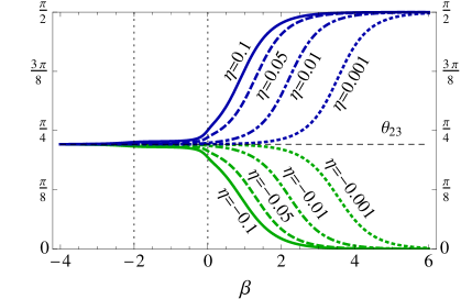
(a) Normal Hierarchy

(b) Inverted Hierarchy

Figure 8: The $\beta$-dependence of $\theta_{23}^{\prime}$ for the (a) normal and (b) inverted hierarchies for several values of $\eta$ with $s_{23}^{2}=0.4$.

To summarize what we have learned, inclusion of the $\hat{a}\eta M_{\eta}$ term in the effective Hamiltonian shifts $\theta_{23}$ to $\theta_{23}^{\prime}=\theta_{23}+\chi$ for the $\delta m^{2}_{31}>0$ case, and to $\theta_{23}^{\prime}=\theta_{23}+\psi$ for the $\delta m^{2}_{31}<0$ case. For both cases, $\theta_{23}^{\prime}$ can be calculated directly without calculating $\chi$ or $\psi$ first via the expression

$$\tan 2\theta_{23}^{\prime}\;\approx\;\dfrac{[\delta m^{2}_{31}c_{13}^{2}-\delta m^{2}_{21}(c_{12}^{2}-s_{12}^{2}s_{13}^{2})]\sin 2\theta_{23}}{[\delta m^{2}_{31}c_{13}^{2}-\delta m^{2}_{21}(c_{12}^{2}-s_{12}^{2}s_{13}^{2})]\cos 2\theta_{23}-2\hat{a}\eta}\;.$$ (203)

Note that as $\beta$ is increased, $\theta_{23}^{\prime}$ runs toward $\dfrac{\pi}{2}$ if $\delta m^{2}_{31}\eta>0$, while it runs toward $0$ if $\delta m^{2}_{31}\eta<0$. The $\beta$-dependence of $\theta_{23}^{\prime}$ is shown in Fig. 8. The CP-violating phase $\delta$ is unaltered and maintains its vacuum value.

The running of the effective mass-squared differences are also modified in the range $\beta\gtrsim 0$. For the $\delta m^{2}_{31}>0$ case, $\lambda_{1}$ and $\lambda_{2}$ show extra running, while for the $\delta m^{2}_{31}<0$ case, it is $\lambda_{1}$ and $\lambda_{3}$ that show extra running, cf. Figs. 6 and 7.

3.5 Discussion at the Probability Level

So far we have focused our attention on how the flavor-diagonal NSI parameter $\eta$ modifies the running of the effective mass-squared differences, mixing angles, and CP-violating phase as functions of $\hat{a}=a(1+\zeta)$ for the neutrinos. We derived simple analytical expressions for these effective parameters using the Jacobi method. We have discussed the running of these effective neutrino oscillation parameters for both the normal ($\delta m^{2}_{31}>0$) and inverted ($\delta m^{2}_{31}<0$) neutrino mass hierarchies. The modifications induced by $\eta$ and $\zeta$ in the running of effective oscillation parameters in the case of anti-neutrino are discussed in detail in appendix A. At this point, we look at how these lepton-flavor-conserving NSI parameters alter the neutrino oscillation probabilities for various appearance and disappearance channels.

In the three-flavor scenario, the neutrino oscillation probabilities in vacuum for the disappearance channel (initial and final flavors are same) take the form

$$P(\nu_{\alpha}\rightarrow\nu_{\alpha}) = 1-4\,|U_{\alpha 2}|^{2}\left(1-|U_{\alpha 2}|^{2}\right)\sin^{2}\frac{\Delta_{21}}{2}-4\,|U_{\alpha 3}|^{2}\left(1-|U_{\alpha 3}|^{2}\right)\sin^{2}\frac{\Delta_{31}}{2}$$ (205)

$$\phantom{1}+2\,|U_{\alpha 2}|^{2}|U_{\alpha 3}|^{2}\left(4\sin^{2}\frac{\Delta_{21}}{2}\sin^{2}\frac{\Delta_{31}}{2}+\sin\Delta_{21}\sin\Delta_{31}\right)\;,$$

and for the appearance channel (initial and final flavors are different) we have

$$P(\nu_{\alpha}\rightarrow\nu_{\beta}) = 4\,|U_{\alpha 2}|^{2}|U_{\beta 2}|^{2}\sin^{2}\frac{\Delta_{21}}{2}+4\,|U_{\alpha 3}|^{2}|U_{\beta 3}|^{2}\sin^{2}\frac{\Delta_{31}}{2}$$ (208)

$$+2\;\Re\left(U^{*}_{\alpha 3}U_{\beta 3}U_{\alpha 2}U^{*}_{\beta 2}\right)\left(4\sin^{2}\frac{\Delta_{21}}{2}\sin^{2}\frac{\Delta_{31}}{2}+\sin\Delta_{21}\sin\Delta_{31}\right)$$

$$-4\,\Im\left(U^{*}_{\alpha 3}U_{\beta 3}U_{\alpha 2}U^{*}_{\beta 2}\right)\left(\sin^{2}\frac{\Delta_{21}}{2}\sin\Delta_{31}-\sin^{2}\frac{\Delta_{31}}{2}\sin\Delta_{21}\right)\;.$$

In the above equations, we define

$$\Delta_{ij}\;\equiv\;\dfrac{\delta m_{ij}^{2}}{2E}L\;=\;2.534\;\biggl{(}\dfrac{\delta m_{ij}^{2}}{\mathrm{eV}^{2}}\biggr{)}\biggl{(}\dfrac{\mathrm{GeV}}{E}\biggr{)}\biggl{(}\dfrac{L}{\mathrm{km}}\biggr{)}\;,\quad\delta m_{ij}^{2}\,\equiv\,m_{i}^{2}-m_{j}^{2}\;.$$ (209)

The transition probabilities in Eq. (205) and Eq. (208) contain several elements of the PMNS matrix $U$ which are expressed in terms of three mixing angles $\theta_{12}$, $\theta_{23}$, $\theta_{13}$, and a CP-violating phase $\delta$ as shown in Eq. (147). The oscillation probabilities for the anti-neutrinos are obtained by replacing $U_{\alpha i}$ with its complex conjugate.

The neutrino oscillation probabilities in the presence of matter are obtained by replacing the vacuum expressions of the elements of the mixing matrix $U$ and the mass-square differences $\Delta_{ij}$ with their effective ‘running’ values in matter Wolfenstein:1977ue ; Mikheev:1986gs ; Mikheev:1986wj :

$$U_{\alpha i}\;\rightarrow\;\overset{\lower 1.0pt\hbox{$\scriptstyle{\sim}$}}{U}_{\alpha i}\;(\theta_{12}\rightarrow\theta_{12}^{\prime},\theta_{13}\rightarrow\theta_{13}^{\prime},\theta_{23}\rightarrow\theta_{23}^{\prime})\;,\quad\Delta_{ij}\;\rightarrow\;\overset{\lower 1.0pt\hbox{$\scriptstyle{\sim}$}}{\Delta}_{ij}=\dfrac{\lambda_{i}-\lambda_{j}}{2E}L\;,$$ (210)

and for the anti-neutrinos

$$U_{\alpha i}\;\rightarrow\;\overset{\lower 1.0pt\hbox{$\scriptstyle{\backsim}$}}{U}_{\alpha i}\;(\theta_{12}\rightarrow\overline{\theta}_{12}^{\prime},\theta_{13}\rightarrow\overline{\theta}_{13}^{\prime},\theta_{23}\rightarrow\overline{\theta}_{23}^{\prime})\;,\quad\Delta_{ij}\;\rightarrow\;\overset{\lower 1.0pt\hbox{$\scriptstyle{\backsim}$}}{\Delta}_{ij}=\dfrac{\overline{\lambda}_{i}-\overline{\lambda}_{j}}{2E}L\;.$$ (211)

To demonstrate the accuracy (or lack thereof in special cases) of our approximate analytical results, we compare the oscillation probabilities calculated with our approximate effective running mixing angles and mass-squared differences with those calculated numerically for the same baseline and line-averaged constant matter density along it. For the mixing angles and mass-squared differences in vacuum, we use the benchmark values from Ref. GonzalezGarcia:2012sz as listed in Table 1. In some plots, we take different values of $\sin^{2}\theta_{23}$ and $\delta$ which we mention explicitly in the figure legends and captions. In this paper, all the plots (except in appendix B) are generated considering the line-averaged constant matter density for a given baseline which has been estimated using the Preliminary Reference Earth Model (PREM) PREM:1981 . In appendix B, we compare the exact numerical probabilities with line-averaged constant Earth density and varying Earth density profile for 8770 km and 10000 km baselines.

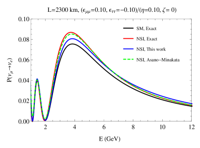
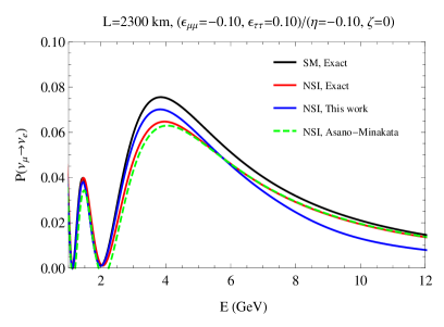
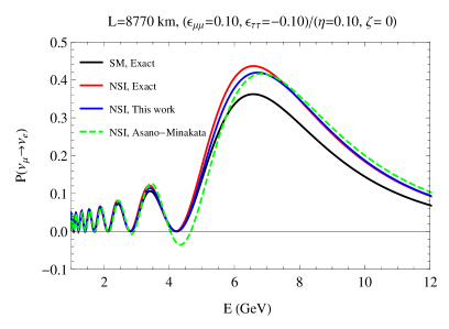
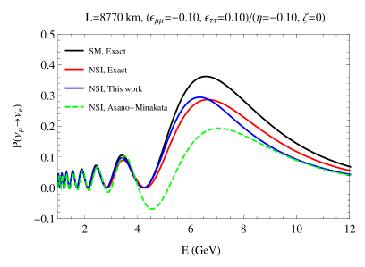
Figure 9: $\nu_{\mu}\rightarrow\nu_{e}$ transition probability as a function of neutrino energy $E$ in GeV for 2300 km (8770 km) baseline in upper (lower) panels. We compare the analytical expressions of this work and Asano-Minakata Asano:2011nj against the exact numerical result assuming $\eta=0.1,\zeta=0$ (left panels) and $\eta=-0.1,\zeta=0$ (right panels). The solid black curves portray the standard three-flavor oscillation probabilities in matter without NSI’s. In all the panels, we consider $\theta_{23}=40^{\circ}$, $\delta=0^{\circ}$, and normal mass hierarchy.

In Fig. 9, we present our approximate $\nu_{\mu}\rightarrow\nu_{e}$ oscillation probabilities (blue curves) as a function of the neutrino energy against the exact numerical results (red curves) considering $\eta=0.1$, $\zeta=0$ (left panels) and $\eta=-0.1$, $\zeta=0$ (right panels). The upper panels are drawn for the baseline of $L=2300\,\mathrm{km}$, which corresponds to the distance between CERN and Pyhäsalmi Agarwalla:2011hh ; Stahl:2012exa ; Agarwalla:2014tca with the line-averaged constant matter density of $\rho=3.54\,\mathrm{g/cm^{3}}$. In the lower panels, we give the probabilities for the baseline of $L=8770\,\mathrm{km}$, which is the distance from CERN to Kamioka Agarwalla:2012zu assuming $\rho=4.33\,\mathrm{g/cm^{3}}$. Here, in all the panels, we assume $\sin^{2}\theta_{23}=0.41~{}(\theta_{23}=40^{\circ})$, $\delta=0^{\circ}$, and normal mass hierarchy ($\delta m^{2}_{31}>0$). To see the differences in the oscillation probability caused by the NSI parameters, we also give the exact numerical SM three-flavor oscillation probabilities in matter in the absence of NSI’s which are depicted by the solid black curves with figure legend ‘SM, Exact.’ It has been already shown in Ref. Agarwalla:2013tza that our approximate expressions for the $\eta=0$ case match extremely well with the exact numerical results for all these baselines and energies. We also compare our results with the approximate expressions of Asano and Minakata Asano:2011nj (dashed green curves). The correspondence between our $\eta$ and $\zeta$ and the NSI parameters $\varepsilon_{ee}$, $\varepsilon_{\mu\mu}$, and $\varepsilon_{\tau\tau}$ used in Refs. Asano:2011nj ; Rahman:2015vqa can be obtained via Eqs. (7), (13), and (15) which suggest the changes : $a\rightarrow\hat{a}\equiv a(1+\zeta)$, $\varepsilon_{ee}\rightarrow 0$, $\varepsilon_{\mu\mu}\rightarrow\eta$, and $\varepsilon_{\tau\tau}\rightarrow-\eta$. We can see from Fig. 9 that for the 2300 km baseline, the Asano-Minakata expressions give better matches compared to our results, while for the 8770 km baseline, our expressions agree better with the exact numerical results.

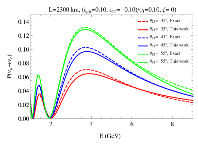
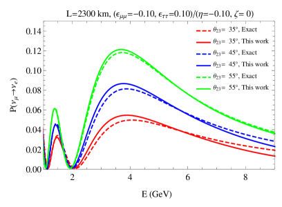
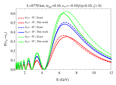
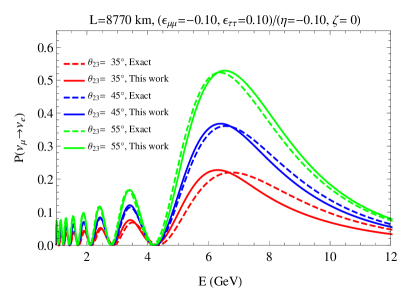
Figure 10: Comparison of our analytical expressions (solid curves) to the exact numerical results (dashed curves) for various values of $\theta_{23}$ assuming $\delta=0^{\circ}$ and $\delta m^{2}_{31}>0$. Upper (lower) panels are for 2300 km (8770 km) baseline.

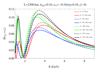
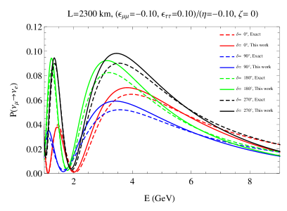
Figure 11: Comparison of our analytical expressions (solid curves) to the exact numerical results (dashed curves) for four different values of the CP-violating phase $\delta$ at 2300 km assuming $\theta_{23}=40^{\circ}$ and $\delta m^{2}_{31}>0$.

The accuracy of our analytical approximations as compared to the exact numerical results for different vacuum values of $\theta_{23}$ is demonstrated in Fig. 10. Here we consider the minimum (35^∘) and maximum (55^∘) values of $\theta_{23}$ which are allowed in the 3$\sigma$ range GonzalezGarcia:2012sz . We also present the results for the maximal mixing choice. All the plots in Fig. 10 have been generated assuming $\delta=0^{\circ}$ and normal mass hierarchy ($\delta m^{2}_{31}>0$). We consider the same choices of $\eta$ and $\zeta$ as in Fig. 9 and results are given for 2300 km (upper panels) and 8770 km (lower panels) baselines. As is evident, our approximation provides satisfactory match with exact numerical results for different values of $\theta_{23}$.

Fig. 11 compares our approximate probability expressions (solid curves) against the exact numerical results (dashed curves) assuming four different values of the CP-violating phase $\delta$ (0, 90, 180, and 270 degrees) at 2300 km. Here, we consider $\theta_{23}=40^{\circ}$ and $\delta m^{2}_{31}>0$. These plots clearly show that our approximate expressions work quite well even for non-zero $\delta$ and can predict almost accurate $L/E$ patterns of the oscillation probability for finite $\delta$ and $\eta$. It also suggests that one can explain qualitatively the possible correlations and degeneracies between $\delta$ and $\eta$ using these analytical expressions which cannot be tackled with numerical studies.

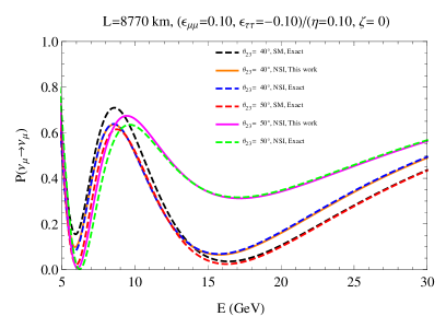
(a) $\eta=0.1,\zeta=0$

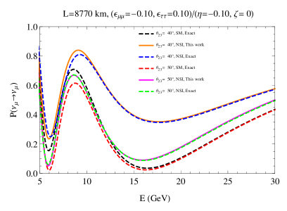
(b) $\eta=-0.1,\zeta=0$

Figure 12: $\nu_{\mu}\rightarrow\nu_{\mu}$ survival probability as a function of neutrino energy $E$ in GeV for two different values of $\theta_{23}$ at 8770 km baseline. Comparison between the analytical and numerical results assuming $\eta=0.1,\zeta=0$ (left panel) and $\eta=-0.1,\zeta=0$ (right panel). The standard three-flavor oscillation probabilities in matter without NSI’s are also shown. In both the panels, we assume $\delta=0^{\circ}$ and $\delta m^{2}_{31}>0$.

In Fig. 12, we plot the $\nu_{\mu}\rightarrow\nu_{\mu}$ survival probability in the presence of NSI for two different vacuum values of $\theta_{23}$ (40^∘ and 50^∘) at 8770 km. We show the matching between the analytical and numerical results assuming $\eta=0.1,\zeta=0$ (left panel) and $\eta=-0.1,\zeta=0$ (right panel). We also give the exact numerical standard three-flavor oscillation probabilities in matter without NSI’s so that one can compare them with the finite $\eta$ case. In both the panels, we assume $\delta=0^{\circ}$ and $\delta m^{2}_{31}>0$. Fig. 12 shows that our approximate expressions match quite nicely with the numerical results. Note that at higher energies, the impact of NSI’s are quite large in the $\nu_{\mu}\rightarrow\nu_{\mu}$ survival channel and there is a substantial difference in the standard and NSI probabilities for both the choices of $\theta_{23}$ which can be probed in future long-baseline Kopp:2008ds ; Coloma:2011rq and atmospheric Chatterjee:2014gxa ; Mocioiu:2014gua ; Choubey:2014iia neutrino oscillation experiments.

Another important point to be noted that in the absence of NSI, the standard probability curves for both the values of $\theta_{23}$ almost overlap with each other at higher energies, whereas with NSI, there is a large separation between them. It immediately suggests that the corrections in the probability expressions due to the NSI terms depend significantly on whether the vacuum value of $\theta_{23}$ lies below or above 45^∘ Fogli:1996pv . Fig. 12 also indicates that there are degeneracies between the octant of $\theta_{23}$ and the sign of NSI parameter $\eta$ for a given choice of hierarchy. For an example, $P_{\mu\mu}(\theta_{23}=50^{\circ},\eta=0.1)$ in the left panel is almost same with $P_{\mu\mu}(\theta_{23}=40^{\circ},\eta=-0.1)$ in the right panel for the energies above 12 GeV or so. Again, $P_{\mu\mu}(\theta_{23}=40^{\circ},\eta=0.1)$ in the left panel matches quite well with $P_{\mu\mu}(\theta_{23}=50^{\circ},\eta=-0.1)$ in the right panel. These kinds of degeneracies can be well explained qualitatively with the help of our analytical expressions. We discuss this issue in detail in the next section which is one of the highlights of this work.

4 Possible Applications of Analytical Expressions

In this section, we discuss the utility of our analytical probability expressions to determine the conditions for which the impact of the NSI parameter $\eta$ becomes significant. We also give simple and compact analytical expressions to show the possible correlations and degeneracies between $\theta_{23}$ and $\eta$ under such situations. We begin our discussion with electron neutrinos.

4.1 $\nu_{e}\rightarrow\nu_{\alpha}$ Oscillation Channels

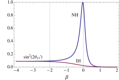
(a) Normal and Inverted Hierarchy

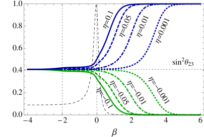
(b) Normal Hierarchy

Figure 13: $\beta$-dependence of (a) $\sin^{2}(2\theta^{\prime}_{13})$ for the normal ($\delta m^{2}_{31}>0$) and inverted ($\delta m^{2}_{31}<0$) hierarchies, and (b) that of $s^{\prime 2}_{23}$ for various values of $\eta$ for the normal hierarchy case. The dashed peak in (b) indicates the behavior of $\sin^{2}(2\theta^{\prime}_{13})$ when $\delta m^{2}_{31}>0$.

Let us first consider the $\nu_{e}\rightarrow\nu_{\alpha}$ ($\alpha=e,\mu,\tau$) oscillation channels in matter in the presence of the NSI parameter $\eta$. Since we expect the effect of $\eta$ to become important in the range $\beta\gtrsim 0$, we set $s^{\prime}_{12}\approx 1$, $c^{\prime}_{12}\approx 0$ (which is valid in the range $\beta\gg-2$, see Fig. 2(a)), which leads to the following simple expressions:

$$\overset{\lower 1.0pt\hbox{$\scriptstyle{\sim}$}}{P}(\nu_{e}\rightarrow\nu_{e}) \approx 1-\sin^{2}(2\theta^{\prime}_{13})\;\sin^{2}\dfrac{\overset{\lower 1.0pt\hbox{$\scriptstyle{\sim}$}}{\Delta}_{32}}{2}\;,$$ (212)

$$\overset{\lower 1.0pt\hbox{$\scriptstyle{\sim}$}}{P}(\nu_{e}\rightarrow\nu_{\mu}) \approx s^{\prime 2}_{23}\,\sin^{2}(2\theta^{\prime}_{13})\;\sin^{2}\dfrac{\overset{\lower 1.0pt\hbox{$\scriptstyle{\sim}$}}{\Delta}_{32}}{2}\;,$$ (213)

$$\overset{\lower 1.0pt\hbox{$\scriptstyle{\sim}$}}{P}(\nu_{e}\rightarrow\nu_{\tau}) \approx c^{\prime 2}_{23}\,\sin^{2}(2\theta^{\prime}_{13})\;\sin^{2}\dfrac{\overset{\lower 1.0pt\hbox{$\scriptstyle{\sim}$}}{\Delta}_{32}}{2}\;.$$ (214)

Recall that when $\delta m^{2}_{31}>0$, the effective mixing angle $\theta_{13}^{\prime}$ increases monotonically toward $\pi/2$, going through $\pi/4$ around $\beta\sim 0$, while in the $\delta m^{2}_{31}<0$ case, it decreases monotonically toward $0$, cf. Fig. 3(b). This will cause $\sin^{2}(2\theta^{\prime}_{13})$ to peak prominently around $\beta\sim 0$ for the normal hierarchy case, but not for the inverted hierarchy case as shown in Fig. 13(a). As discussed in Ref. Agarwalla:2013tza , demanding that $\sin^{2}(\overset{\lower 1.0pt\hbox{$\scriptstyle{\sim}$}}{\Delta}_{32}/2)$ also peaks at the same energy leads to the requirements of $L\sim 10000\,\mathrm{km}$ and $E\sim 7\,\mathrm{GeV}$. Thus, measuring $\overset{\lower 1.0pt\hbox{$\scriptstyle{\sim}$}}{P}(\nu_{e}\rightarrow\nu_{e})$ survival probability at this baseline and energy will allow us to discriminate between the normal and inverted mass hierarchies irrespective of the value of $\theta_{23}$ Agarwalla:2006gz . Also, around $\beta\sim 0$, $\overset{\lower 1.0pt\hbox{$\scriptstyle{\sim}$}}{\Delta}_{32}$ is not affected by $\eta$ provided $\eta\lesssim 0.1$ (see middle and bottom panels of Fig. 6), allowing this channel to determine the mass hierarchy free from any NSI effect.

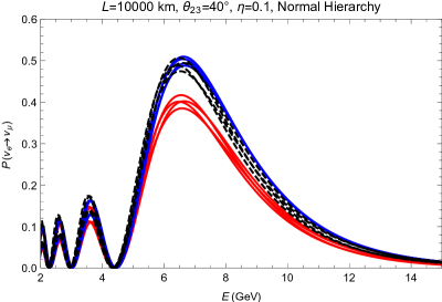
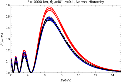
Figure 14: The oscillation probabilities (a) $P(\nu_{e}\rightarrow\nu_{\mu})$ and (b) $P(\nu_{e}\rightarrow\nu_{\tau})$ for the normal hierarchy case with $s_{23}^{2}=0.4$. The red lines are the standard oscillation probabilities with $\eta=0$ and $\delta=0,90,180,$ and $270$ degrees. The blue lines are our approximate analytical results with $\eta=0.1$ and the black dashed lines are the numerically calculated probabilities with $\eta=0.1$. In both the cases, we plot the probabilities for four values of $\delta=0,90,180,$ and $270$ degrees. Note that $P(\nu_{e}\rightarrow\nu_{\mu})$ is enhanced by about $\eta$, while $P(\nu_{e}\rightarrow\nu_{\tau})$ is suppressed by an equal amount.

To see the effect of $\eta$, we need to observe the running of $\theta_{23}^{\prime}$. This could be visible in the $\nu_{e}\rightarrow\nu_{\mu}$ and $\nu_{e}\rightarrow\nu_{\tau}$ appearance channels for the normal hierarchy case as a change in the heights of the oscillation peaks around $E\sim 7\,\mathrm{GeV}$ provided $\theta^{\prime}_{23}$ deviates sufficiently from the vacuum value of $\theta_{23}$ at that energy. The running of $s^{\prime 2}_{23}$ for various values of $\eta$ is depicted in Fig. 13(b). At $\hat{a}\sim\delta m^{2}_{31}$, Eq. (203) tells us that

$$s^{\prime 2}_{23}\;\approx\;s^{2}_{23}+\eta\;,$$ (215)

showing the possible shift in $\theta_{23}$ due to $\eta$ in a simple and compact fashion which clearly establishes the merit of our analytical approximation. Eq. (215) also shows compactly possible correlations and degeneracies between $\theta_{23}$ and $\eta$. Such correlations and degeneracies could also be found numerically, but the reason for those features will not be so transparent. Note that Eq. (215) suggests that a positive value of $\eta$ would enhance $\overset{\lower 1.0pt\hbox{$\scriptstyle{\sim}$}}{P}(\nu_{e}\rightarrow\nu_{\mu})$ while suppressing $\overset{\lower 1.0pt\hbox{$\scriptstyle{\sim}$}}{P}(\nu_{e}\rightarrow\nu_{\tau})$, and a negative $\eta$ would do the opposite. Fig. 14 confirms this feature where we plot the $\nu_{e}\rightarrow\nu_{\mu}$ ($\nu_{e}\rightarrow\nu_{\tau}$) transition probability in the left (right) panel. In both panels, the standard oscillation probabilities in matter without NSI’s for four different values of CP phase $\delta$ are given by the solid red lines. Blue lines (black dashed lines) depict the approximate analytical (exact numerical) probabilities with $\eta=0.1$ and four different values of $\delta$. Fig. 14 infers that the effect of $\eta$ is visible in these channels provided the vacuum value of $\theta_{23}$ is sufficiently well known and $\eta$ is also large enough.

4.2 $\nu_{\mu}\rightarrow\nu_{\alpha}$ Oscillation Channels

Next, let us consider $\nu_{\mu}\rightarrow\nu_{\alpha}$ $(\alpha=\mu,\tau)$ oscillation channels. In addition to assuming $\beta\gg-2$, which allows us to set $s^{\prime}_{12}\approx 1$, $c^{\prime}_{12}\approx 0$, we further restrict our consideration to the range $\beta\gtrsim 1$, which allows us to set $s^{\prime}_{13}\approx 1$, $c^{\prime}_{13}\approx 0$ or $s^{\prime}_{13}\approx 0$, $c^{\prime}_{13}\approx 1$ depending on whether $\delta m^{2}_{31}>0$ or $\delta m^{2}_{31}<0$ (see Fig. 3(b)). With these conditions, we obtain the following simple expressions:

$$\overset{\lower 1.0pt\hbox{$\scriptstyle{\sim}$}}{P}({\nu}_{\mu}\rightarrow{\nu}_{\mu}) \approx 1-4s_{13}^{\prime 2}s_{23}^{\prime 2}(1-s_{13}^{\prime 2}s_{23}^{\prime 2})\sin^{2}\frac{\overset{\lower 1.0pt\hbox{$\scriptstyle{\sim}$}}{\Delta}_{21}}{2}-4c_{13}^{\prime 2}s_{23}^{\prime 2}(1-c_{13}^{\prime 2}s_{23}^{\prime 2})\sin^{2}\frac{\overset{\lower 1.0pt\hbox{$\scriptstyle{\sim}$}}{\Delta}_{31}}{2}$$ (221)

$$\qquad\qquad\quad+2s_{13}^{\prime 2}c_{13}^{\prime 2}s_{23}^{\prime 4}\left(4\sin^{2}\dfrac{\overset{\lower 1.0pt\hbox{$\scriptstyle{\sim}$}}{\Delta}_{21}}{2}\sin^{2}\dfrac{\overset{\lower 1.0pt\hbox{$\scriptstyle{\sim}$}}{\Delta}_{31}}{2}+\sin\overset{\lower 1.0pt\hbox{$\scriptstyle{\sim}$}}{\Delta}_{21}\sin\overset{\lower 1.0pt\hbox{$\scriptstyle{\sim}$}}{\Delta}_{31}\right)$$

$$\xrightarrow{\beta\gtrsim 1}\;\left\{\begin{array}[]{ll}1-\sin^{2}(2\theta_{23}^{\prime})\sin^{2}\dfrac{\overset{\lower 1.0pt\hbox{$\scriptstyle{\sim}$}}{\Delta}_{21}}{2}&\qquad(\delta m^{2}_{31}>0)\\ 1-\sin^{2}(2\theta_{23}^{\prime})\sin^{2}\dfrac{\overset{\lower 1.0pt\hbox{$\scriptstyle{\sim}$}}{\Delta}_{31}}{2}&\qquad(\delta m^{2}_{31}<0)\end{array}\right.\;,$$

$$\overset{\lower 1.0pt\hbox{$\scriptstyle{\sim}$}}{P}(\nu_{\mu}\rightarrow\nu_{\tau}) \approx \sin(2\theta^{\prime}_{23})\left[s^{\prime 4}_{13}\sin^{2}\frac{\overset{\lower 1.0pt\hbox{$\scriptstyle{\sim}$}}{\Delta}_{21}}{2}+c^{\prime 4}_{13}\sin^{2}\frac{\overset{\lower 1.0pt\hbox{$\scriptstyle{\sim}$}}{\Delta}_{31}}{2}\right.$$ (226)

$$\qquad\qquad\quad\left.+\;s_{13}^{\prime 2}c^{\prime 2}_{13}\left(2\sin^{2}\frac{\overset{\lower 1.0pt\hbox{$\scriptstyle{\sim}$}}{\Delta}_{21}}{2}\sin^{2}\frac{\overset{\lower 1.0pt\hbox{$\scriptstyle{\sim}$}}{\Delta}_{31}}{2}+\dfrac{1}{2}\sin\overset{\lower 1.0pt\hbox{$\scriptstyle{\sim}$}}{\Delta}_{21}\sin\overset{\lower 1.0pt\hbox{$\scriptstyle{\sim}$}}{\Delta}_{31}\right)\right]\qquad$$

$$\xrightarrow{\beta\gtrsim 1}\;\left\{\begin{array}[]{ll}\sin^{2}(2\theta_{23}^{\prime})\sin^{2}\dfrac{\overset{\lower 1.0pt\hbox{$\scriptstyle{\sim}$}}{\Delta}_{21}}{2}&\qquad(\delta m^{2}_{31}>0)\\ \sin^{2}(2\theta_{23}^{\prime})\sin^{2}\dfrac{\overset{\lower 1.0pt\hbox{$\scriptstyle{\sim}$}}{\Delta}_{31}}{2}&\qquad(\delta m^{2}_{31}<0)\end{array}\right.\;.$$

In the absence of $\eta$, $\theta^{\prime}_{23}$ does not run and $\sin^{2}(2\theta^{\prime}_{23})$ will maintain its vacuum value close to one. In the presence of a non-zero $\eta$, however, $\theta^{\prime}_{23}$ will run towards either $\dfrac{\pi}{2}$ or $0$ depending on the sign of $\delta m^{2}_{31}\eta$, as was shown in Fig. 8, and $\sin^{2}(2\theta^{\prime}_{23})$ will run toward zero in both cases. This is depicted in Fig. 15.

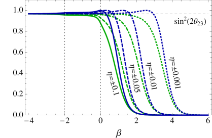
(a) Normal Hierarchy

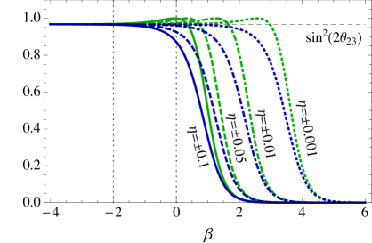
(b) Inverted Hierarchy

Figure 15: The running of $\sin^{2}(2\theta^{\prime}_{23})$ for various values of $\eta$ for the (a) normal and (b) inverted mass hierarchies with $s^{2}_{23}=0.4$. The blue/green lines indicate positive/negative values of $\eta$.

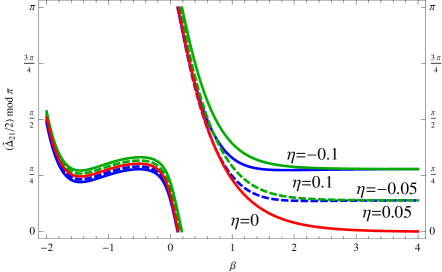
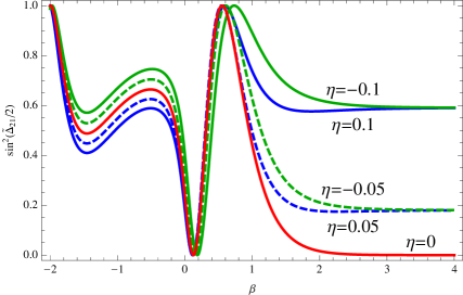
Figure 16: The running of (a) $\overset{\lower 1.0pt\hbox{$\scriptstyle{\sim}$}}{\Delta}_{21}/2$ and (b) $\sin^{2}(\overset{\lower 1.0pt\hbox{$\scriptstyle{\sim}$}}{\Delta}_{21}/2)$ for various values of $\eta$ for the normal hierarchy case with $L=10,000\,\mathrm{km}$ and $\rho=4.53\,\mathrm{g/cm^{3}}$. The blue/green lines indicate positive/negative values of $\eta$, while the red lines are drawn for $\eta=0$ case.

Let us see how the $\Delta$ factors in Eq. (221) and Eq. (226) behave in the range $\beta\gtrsim 1$. For the normal hierarchy case, we have

$$\delta\lambda_{21}\;\approx\;\left\{\begin{array}[]{llll}\lambda_{X+}^{\prime\prime\prime}&-\;\lambda_{X-}^{\prime\prime\prime}&\approx\;2\hat{a}|\eta|&\qquad(\eta\neq 0)\\ \lambda_{-}^{\prime\prime}&-\;\lambda_{-}^{\prime}&\approx\;\delta m^{2}_{31}c_{13}^{2}&\qquad(\eta=0)\end{array}\right.\;,$$ (227)

while for the inverted hierarchy case, they take the form

$$\delta\lambda_{31}\;\approx\;\left\{\begin{array}[]{llll}\lambda_{Y-}^{\prime\prime\prime}&-\;\lambda_{Y+}^{\prime\prime\prime}&\approx\;-2\hat{a}|\eta|&\qquad(\eta\neq 0)\\ \lambda_{-}^{\prime\prime}&-\;\lambda_{-}^{\prime}&\approx\;-|\delta m^{2}_{31}|c_{13}^{2}&\qquad(\eta=0)\end{array}\right.\;.$$ (228)

Since the sign of $\delta\lambda_{ij}$ does not affect the value of $\sin^{2}(\overset{\lower 1.0pt\hbox{$\scriptstyle{\sim}$}}{\Delta}_{ij}/2)$, both mass hierarchies lead to the same asymptotic oscillation probabilities. We will therefore only consider the normal hierarchy case in the following. Recalling (see Eq. (5)) that

$$\hat{a}\;=\;2\sqrt{2}G_{F}N_{e}E\;=\;7.6324\times 10^{-5}(\mathrm{eV}^{2})\left(\dfrac{\rho}{\mathrm{g/cm^{3}}}\right)\left(\dfrac{E}{\mathrm{GeV}}\right)\;,$$ (229)

(where we have set $\zeta=0$) and

$$\overset{\lower 1.0pt\hbox{$\scriptstyle{\sim}$}}{\Delta}_{ij} = 2.534\left(\dfrac{\delta\lambda_{ij}}{\mathrm{eV}^{2}}\right)\left(\dfrac{\mathrm{GeV}}{E}\right)\left(\dfrac{L}{\mathrm{km}}\right)$$ (230)

$$= 1.934\left(\dfrac{\delta\lambda_{ij}}{\hat{a}}\right)\left(\dfrac{\rho}{\mathrm{g/cm^{3}}}\right)\left(\dfrac{L}{10^{4}\,\mathrm{km}}\right)\;,$$ (231)

we find

$$\dfrac{\overset{\lower 1.0pt\hbox{$\scriptstyle{\sim}$}}{\Delta}_{21}}{2}\;=\;\dfrac{\delta\lambda_{21}}{4E}L$$ (232)

$$\approx \left\{\begin{array}[]{lll}2\,|\eta|\left(\dfrac{\rho}{\mathrm{g/cm^{3}}}\right)\left(\dfrac{L}{10^{4}\,\mathrm{km}}\right)&&\qquad(\eta\neq 0)\\ \left(\dfrac{\delta m^{2}_{31}}{\hat{a}}\right)\left(\dfrac{\rho}{\mathrm{g/cm^{3}}}\right)\left(\dfrac{L}{10^{4}\,\mathrm{km}}\right)&\approx\;30\left(\dfrac{\mathrm{GeV}}{E}\right)\left(\dfrac{L}{10^{4}\,\mathrm{km}}\right)&\qquad(\eta=0)\end{array}\right.\;.$$ (235)

Therefore, for fixed baseline $L$ and matter density $\rho$, as the neutrino energy $E$ is increased, $\overset{\lower 1.0pt\hbox{$\scriptstyle{\sim}$}}{\Delta}_{21}/2$ damps to zero when $\eta=0$, but asymptotes to a constant value proportional to $|\eta|$ when $\eta\neq 0$. This is demonstrated in Fig. 16 for the baseline $L=10000\,\mathrm{km}$ with average matter density $\rho=4.53\,\mathrm{g/cm^{3}}$. Consequently, when $\eta=0$, the factor $\sin^{2}(2\theta_{23}^{\prime})$ stays constant while $\sin^{2}(\overset{\lower 1.0pt\hbox{$\scriptstyle{\sim}$}}{\Delta}_{21}/2)$ damps to zero as we increase $E$, while in the $\eta\neq 0$ case, the factor $\sin^{2}(2\theta_{23}^{\prime})$ damps to zero while $\sin^{2}(\overset{\lower 1.0pt\hbox{$\scriptstyle{\sim}$}}{\Delta}_{21}/2)$ asymptotes to a constant value as $E$ is increased. In either case, the $\nu_{\mu}\rightarrow\nu_{\tau}$ oscillation probability is suppressed at high energy.

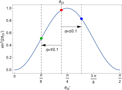
(a) $s^{2}_{23}=0.4$

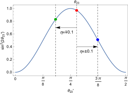
(b) $s^{2}_{23}=0.6$

Figure 17: $\theta_{23}^{\prime}$ and $\sin^{2}(2\theta^{\prime}_{23})$ as a function of positive and negative values of $\eta$ for a fixed $s^{2}_{23}=0.4$ ($s^{2}_{23}=0.6$) in the left (right) panel. The upper (lower) signs are applicable for the normal (inverted) hierarchy case.

The difference between the $\eta=0$ and $\eta\neq 0$ cases could manifest itself at the $\nu_{\mu}\rightarrow\nu_{\tau}$ oscillation peak which happens at

$$\dfrac{\pi}{2}\;=\;\dfrac{\overset{\lower 1.0pt\hbox{$\scriptstyle{\sim}$}}{\Delta}_{21}}{2}\quad\rightarrow\quad E\;\approx\;20\,\mathrm{GeV}\;,\;\beta\;\approx\;0.6\;,$$ (237)

for $L=10000\,\mathrm{km}$, $\rho=4.53\,\mathrm{g/cm^{3}}$ case. $\beta\approx 0.6$ is on the borderline of the applicability of our $\beta\gtrsim 1$ approximation. Nevertheless, let us examine what our approximation suggests. Expanding Eq. (203) for small $\hat{a}\eta$, we find

$$\theta^{\prime}_{23}\;=\;\theta_{23}+\dfrac{\hat{a}\sin(2\theta_{23})}{\delta m^{2}_{31}c_{13}^{2}}\eta+\cdots$$ (238)

which at $\beta\approx 0.6$ yields

$$\theta^{\prime}_{23}\;\approx\;\theta_{23}\pm 3\eta\;.$$ (239)

In the above equation, upper (lower) sign is applicable for the normal (inverted) hierarchy case. It suggests that there is a degeneracy between the choices of sign of $\delta m^{2}_{31}$ and the sign of $\eta$ which give rise to same amount of corrections in $\theta_{23}$. To observe the shift in the oscillation probability, we keep terms up to order $\eta^{2}$ since the linear term is suppressed due to the fact that $\theta_{23}$ is close to $\pi/4$. Therefore, we have

$$\sin(2\theta^{\prime}_{23}) = \sin(2\theta_{23})+2\cos(2\theta_{23})\delta\theta_{23}-2\sin(2\theta_{23})(\delta\theta_{23})^{2}+\cdots$$ (240)

$$\approx \sin(2\theta_{23})\pm 6\cos(2\theta_{23})\eta-18\sin(2\theta_{23})\eta^{2}\;.$$ (241)

For the benchmark value of $s^{2}_{23}$ = 0.4 (0.6) in the lower (higher) octant, above equation can be written as

$$\sin(2\theta^{\prime}_{23})\;\approx\;\left\{\begin{array}[]{llll}\sin(2\theta_{23})\pm\eta-18\eta^{2}\qquad(s^{2}_{23}=0.4)\\ \sin(2\theta_{23})\mp\eta-18\eta^{2}\qquad(s^{2}_{23}=0.6)\end{array}\right.\;,$$ (242)

where upper (lower) signs are for the normal (inverted) hierarchy. The above equations clearly reveal that for a given choice of hierarchy, there are degenerate solutions of the octant of $\theta_{23}$ and the sign of NSI parameter $\eta$ ($s^{2}_{23}=0.4,\eta=\pm 0.1$ and $s^{2}_{23}=0.6,\eta=\mp 0.1$), giving rise to same value of $\sin(2\theta^{\prime}_{23})$. Fig. 17 shows the variation in $\theta_{23}^{\prime}$ and $\sin^{2}(2\theta^{\prime}_{23})$ as a function of positive and negative values of $\eta$ for a fixed $s^{2}_{23}=0.4$ ($s^{2}_{23}=0.6$) in the left (right) panel. The upper (lower) signs correspond to the normal (inverted) hierarchy scenario. We can see from the left panel of Fig. 17 that assuming normal hierarchy and $s^{2}_{23}=0.4$, the value of $\sin^{2}(2\theta^{\prime}_{23})$ gets reduced by substantial amount for $\eta=-0.1$ case as compared to $\eta=0.1$ as given by Eq. (242). It means that negative values of $\eta$, which shifts $\theta_{23}$ further away from $\pi/4$, would lead to a larger suppression of the $\nu_{\mu}\rightarrow\nu_{\tau}$ oscillation probability, and enhancement of the $\nu_{\mu}\rightarrow\nu_{\mu}$ survival probability. The left and right panels of Fig. 18 exactly show this behaviour where we plot the approximate analytical and exact numerical $\nu_{\mu}\rightarrow\nu_{\tau}$ (left panel) and $\nu_{\mu}\rightarrow\nu_{\mu}$ (right panel) probabilities for $\eta=\pm 0.1$ assuming $s^{2}_{23}=0.4$, $\delta m^{2}_{31}>0$ and $L=10000\,\mathrm{km}$, $\rho=4.53\,\mathrm{g/cm^{3}}$. The situation gets reversed completely for cases in which $s^{2}_{23}>0.5$ which is quite evident from the right panel of Fig. 17 where we consider $s^{2}_{23}=0.6$. All these observations in Fig. 17 and Fig. 18 suggest that our approximate calculations are valid.

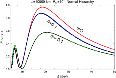
(a) $P(\nu_{\mu}\rightarrow\nu_{\tau})$

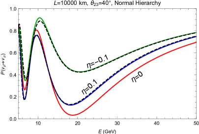
(b) $P(\nu_{\mu}\rightarrow\nu_{\mu})$

Figure 18: (a) $\nu_{\mu}\rightarrow\nu_{\tau}$ and (b) $\nu_{\mu}\rightarrow\nu_{\mu}$ oscillation probabilities for $s^{2}_{23}=0.4$, $L=10,000\,\mathrm{km}$, and $\rho=4.53\,\mathrm{g/cm^{3}}$. The red lines are the standard oscillation probabilities with $\eta=0$. The solid blue (green) lines are our approximate analytical results with $\eta=0.1$ ($\eta=-0.1$). The black dashed lines are the numerically calculated probabilities. In both the panels, we take $\delta=0^{\circ}$ and $\delta m^{2}_{31}>0$.

5 Summary and Conclusions

Analytical studies of the neutrino oscillation probabilities are inevitable to understand how neutrino interactions with matter modify the mixing angles and mass-squared differences in a complicated manner in a three-flavor framework. In previous papers Agarwalla:2013tza ; Honda:2006hp , we showed that the neutrino oscillation probabilities in matter can be well understood if we allow the mixing angles and mass-squared differences in the standard parametrization to ‘run’ with the matter effect parameter $a=2\sqrt{2}G_{F}N_{e}E$, where $N_{e}$ is the electron density in matter and $E$ is the neutrino energy. We managed to derive simple and compact analytical approximations to these running parameters using the Jacobi method. We found that for large $\theta_{13}$, the entire matter effect could be absorbed into the running of the effective mass-squared differences and the effective mixing angles $\theta_{12}$ and $\theta_{13}$, while neglecting the running of the mixing angle $\theta_{23}$ and the CP-violating phase $\delta$.

In this paper, we extended our analysis to study how the running of the neutrino oscillation parameters in matter would be altered in the presence of NSI’s of neutrinos with the matter fermions. Such NSI’s are predicted in most of the new physics models that attempt to explain the non-zero neutrino masses, as well as in a wealth of various other BSM models. There, the NSI’s are simply the effective four-fermion interactions at the energy scales relevant for neutrino oscillation experiments that remain when the heavy mediator fields of the full theory are integrated out. These NSI’s give rise to new neutral-current type interactions of neutrinos (both flavor-conserving and flavor-violating) during their propagation through matter on top of the SM interactions, causing the change in the effective mass matrix for the neutrinos which ultimately affect the running of the oscillation parameters and hence change the oscillation probabilities between different neutrino flavors. These sub-leading new physics effects in the probability due to NSI’s can be probed in upcoming long-baseline and atmospheric neutrino oscillation experiments.

In this work, we restricted our attention to the matter effect of flavor-conserving, non-universal NSI’s of the neutrino, relegating the discussion of the flavor-violating NSI case to a separate paper AgarwallaKaoSunTakeuchi:2015 . The relevant linear combinations of the flavor-diagonal NSI’s were $\eta=(\varepsilon_{\mu\mu}-\varepsilon_{\tau\tau})/2$ and $\zeta=\varepsilon_{ee}-(\varepsilon_{\mu\mu}+\varepsilon_{\tau\tau})/2$, where a non-zero $\zeta$ led to a rescaling of the matter-effect parameter $a\rightarrow\hat{a}=a(1+\zeta)$, while a non-zero $\eta$ led to non-trivial modifications on how the running oscillation parameters depend on $\hat{a}$.

Utilizing the Jacobi method, as in Refs. Agarwalla:2013tza ; Honda:2006hp , we obtained approximate analytical expressions for the effective neutrino oscillation parameters to study how they ‘run’ with the rescaled matter-effect parameter $\hat{a}$, and to explore the role of non-zero $\eta$ in neutrino oscillation. We found that in addition to the two rotations, which were required for the SM matter interaction and were absorbed into effective values of $\theta_{12}$ and $\theta_{13}$, a third rotation was needed to capture the effects of $\eta$, which could be absorbed into the effective value of $\theta_{23}$. Thus, within the neutrino mixing matrix, the effect of $\eta$ appears as a shift in the effective mixing angle $\theta_{23}$, while the SM matter effects show up as shifts in $\theta_{12}$ and $\theta_{13}$. The CP-violating phase $\delta$ remains unaffected and maintains its vacuum value. The running of all the effective neutrino oscillation parameters were presented for both the normal and inverted neutrino mass hierarchies. The changes caused by $\eta$ in the running of the effective oscillation parameters for the anti-neutrino case are discussed in detail in appendix A.

We have also studied the impact of the lepton-flavor-conserving NSI parameters on the neutrino oscillation probabilities for various appearance and the disappearance channels. To demonstrate the accuracy (or lack thereof in special cases) of our approximate analytical expressions, we compared the oscillation probabilities estimated with our approximate effective ‘running’ mixing angles and mass-squared differences with those calculated numerically for the same choices of benchmark oscillation parameters, energy, baseline, and line-averaged constant matter density along it. We found that our approximation provided satisfactory matches with exact numerical results in light of large $\theta_{13}$ for different values of $\theta_{23}$, CP-violating phase $\delta$, and for positive and negative values of the NSI parameter $\eta$. A comparison of our results with the approximate expressions of Asano and Minakata Asano:2011nj for the $\nu_{\mu}\rightarrow\nu_{e}$ appearance channel has also been presented.

Finally, we examined the merit of our analytical probability expressions to identify the situations at which the impact of the NSI’s become compelling. It was found that at higher baselines and energies, the impact of $\eta$ can be quite significant in the $\nu_{\mu}\rightarrow\nu_{\mu}$ survival channel if $|\eta|$ is of the order of its current experimental upper bound. A considerable difference between the SM and NSI probabilities can be seen irrespective of the vacuum value of $\theta_{23}$, and the sign of the NSI parameter $\eta$. We note that this feature may be explorable with the upcoming 50 kiloton magnetized iron calorimeter detector at the India-based Neutrino Observatory (INO), which aims to detect atmospheric neutrinos and anti-neutrinos separately over a wide range of energies and path lengths KhatunChatterjeeThakoreAgarwalla:2015 . Using our analytical approach, we showed in a very simple and compact fashion that the corrections in $\theta_{23}$ due to the $\eta$ depend significantly on whether the vacuum value of $\theta_{23}$ lies below or above 45^∘, suggesting a possible degeneracy between the octant of $\theta_{23}$ and the sign of $\eta$ for a given choice of mass hierarchy.

Acknowledgments

We would like to thank Minako Honda and Naotoshi Okamura for their contributions to Ref. Honda:2006gv , the predecessor to this work. Helpful conversations with Sabya Sachi Chatterjee, Arnab Dasgupta, Shunsaku Horiuchi, Gail McLaughlin, and Matthew Rave are gratefully acknowledged. We thank the referee for useful suggestions. SKA was supported by the DST/INSPIRE Research Grant [IFA-PH-12], Department of Science & Technology, India. TT is grateful for the hospitality of the Kavli-IPMU during his sabbatical year from fall 2012 to summer 2013 where portions of this work was performed, and where he was supported by the World Premier International Research Center Initiative (WPI Initiative), MEXT, Japan.

Appendix A Effective Mixing Angles and Effective Mass-Squared Differences
– Anti-Neutrino Case

In this appendix, we study the matter effect due to the anti-neutrino NSI’s. We again utilize the Jacobi method to estimate how the NSI parameter $\eta$ alters the ‘running’ of the effective mixing angles, effective mass-squared differences, and the effective CP-violating phase $\delta$ in matter for the anti-neutrinos. Like the neutrino case, we also present here a comparison between our approximate analytical probability expressions and exact numerical calculations towards the end of this appendix.

A.1 Differences from the Neutrino Case

For the anti-neutrinos, the effective Hamiltonian is given by

$$\overline{H}_{\eta}\;=\;\overset{\lower 1.0pt\hbox{$\scriptstyle{\backsim}$}}{U}{}^{*}\left[\begin{array}[]{ccc}\overline{\lambda}_{1}&0&0\\ 0&\overline{\lambda}_{2}&0\\ 0&0&\overline{\lambda}_{3}\end{array}\right]\overset{\lower 1.0pt\hbox{$\scriptstyle{\backsim}$}}{U}{}^{T}=\underbrace{U^{*}\left[\begin{array}[]{ccc}0&0&0\\ 0&\delta m^{2}_{21}&0\\ 0&0&\delta m^{2}_{31}\end{array}\right]U^{T}-\hat{a}\underbrace{\left[\begin{array}[]{ccc}1&0&0\\ 0&0&0\\ 0&0&0\end{array}\right]}_{\displaystyle=M_{a}}}_{\displaystyle=\overline{H}_{0}}-\hat{a}\eta\underbrace{\left[\begin{array}[]{ccc}0&0&0\\ 0&1&0\\ 0&0&-1\end{array}\right]}_{\displaystyle=M_{\eta}}\;.$$ (243)

The differences from the neutrino case are the reversal of signs of the CP-violating phase $\delta$ (and thus the complex conjugation of the PMNS matrix $U$), and the matter interaction parameter $\hat{a}=a(1+\zeta)$. We denote the matter effect corrected diagonalization matrix as $\overset{\lower 1.0pt\hbox{$\scriptstyle{\backsim}$}}{U}$ (note the mirror image tilde on top) to distinguish it from that for the neutrinos.

A.2 Diagonalization of the Effective Hamiltonian

A.2.1 Change to the Mass Eigenbasis in Vacuum

Using the matrix $Q_{3}$ from Eq. (32), we begin by partially diagonalize the effective Hamiltonian $\overline{H}_{\eta}$ as

$$\overline{H}_{\eta}^{\prime} = Q_{3}U^{T}\overline{H}_{\eta}U^{*}Q_{3}^{*}$$ (244)

$$= \underbrace{\left[\begin{array}[]{ccc}0&0&0\\ 0&\delta m^{2}_{21}&0\\ 0&0&\delta m^{2}_{31}\end{array}\right]-\hat{a}\underbrace{Q_{3}U^{T}\underbrace{\left[\begin{array}[]{ccc}1&0&0\\ 0&0&0\\ 0&0&0\end{array}\right]}_{\displaystyle M_{a}}U^{*}Q_{3}^{*}}_{\displaystyle\equiv\overline{M}_{a}^{\prime}(\theta_{12},\theta_{13},\theta_{23})}}_{\displaystyle\equiv\overline{H}_{0}^{\prime}}-\hat{a}\eta\underbrace{Q_{3}U^{T}\underbrace{\left[\begin{array}[]{ccc}0&0&0\\ 0&1&0\\ 0&0&-1\end{array}\right]}_{\displaystyle M_{\eta}}U^{*}Q_{3}^{*}}_{\displaystyle\equiv\overline{M}_{\eta}^{\prime}(\theta_{12},\theta_{13},\theta_{23},\delta)}\;,$$ (254)

where

$$\overline{M}^{\prime}_{a}(\theta_{12},\theta_{13},\theta_{23})\;=\;Q_{3}\left[\begin{array}[]{ccc}U_{e1}U_{e1}^{*}&U_{e1}U_{e2}^{*}&U_{e1}U_{e3}^{*}\\ U_{e2}U_{e1}^{*}&U_{e2}U_{e2}^{*}&U_{e2}U_{e3}^{*}\\ U_{e3}U_{e1}^{*}&U_{e3}U_{e2}^{*}&U_{e3}U_{e3}^{*}\end{array}\right]Q_{3}^{*} = \left[\begin{array}[]{ccc}c_{12}^{2}c_{13}^{2}&c_{12}s_{12}c_{13}^{2}&c_{12}c_{13}s_{13}\\ c_{12}s_{12}c_{13}^{2}&s_{12}^{2}c_{13}^{2}&s_{12}c_{13}s_{13}\\ c_{12}c_{13}s_{13}&s_{12}c_{13}s_{13}&s_{13}^{2}\end{array}\right]$$ (261)

$$= M^{\prime}_{a}(\theta_{12},\theta_{13},\theta_{23})\;,\phantom{\Bigg{|}}$$ (262)

and

$$\overline{M}^{\prime}_{\eta}(\theta_{12},\theta_{13},\theta_{23},\delta) = Q_{3}\left\{\left[\begin{array}[]{ccc}U_{\mu 1}U_{\mu 1}^{*}&U_{\mu 1}U_{\mu 2}^{*}&U_{\mu 1}U_{\mu 3}^{*}\\ U_{\mu 2}U_{\mu 1}^{*}&U_{\mu 2}U_{\mu 2}^{*}&U_{\mu 2}U_{\mu 3}^{*}\\ U_{\mu 3}U_{\mu 1}^{*}&U_{\mu 3}U_{\mu 2}^{*}&U_{\mu 3}U_{\mu 3}^{*}\end{array}\right]-\left[\begin{array}[]{ccc}U_{\tau 1}U_{\tau 1}^{*}&U_{\tau 1}U_{\tau 2}^{*}&U_{\tau 1}U_{\tau 3}^{*}\\ U_{\tau 2}U_{\tau 1}^{*}&U_{\tau 2}U_{\tau 2}^{*}&U_{\tau 2}U_{\tau 3}^{*}\\ U_{\tau 3}U_{\tau 1}^{*}&U_{\tau 3}U_{\tau 2}^{*}&U_{\tau 3}U_{\tau 3}^{*}\end{array}\right]\right\}Q_{3}^{*}$$ (269)

$$= \left[\begin{array}[]{l}\sin(2\theta_{12})\sin(2\theta_{23})s_{13}\cos\delta+(s_{12}^{2}-c_{12}^{2}s_{13}^{2})\cos(2\theta_{23})\\ (s_{12}^{2}e^{+i\delta}-c_{12}^{2}e^{-i\delta})s_{13}\sin(2\theta_{23})-(1+s_{13}^{2})s_{12}c_{12}\cos(2\theta_{23})\\ -s_{12}c_{13}\sin(2\theta_{23})e^{+i\delta}+c_{12}s_{13}c_{13}\cos(2\theta_{23})\end{array}\right.$$ (281)

$$\qquad\qquad\begin{array}[]{l}(s_{12}^{2}e^{-i\delta}-c_{12}^{2}e^{+i\delta})s_{13}\sin(2\theta_{23})-(1+s_{13}^{2})s_{12}c_{12}\cos(2\theta_{23})\\ -\sin(2\theta_{12})\sin(2\theta_{23})s_{13}\cos\delta+(c_{12}^{2}-s_{12}^{2}s_{13}^{2})\cos(2\theta_{23})\\ \phantom{-}c_{12}c_{13}\sin(2\theta_{23})e^{+i\delta}+s_{12}s_{13}c_{13}\cos(2\theta_{23})\end{array}$$

$$\qquad\qquad\qquad\qquad\left.\begin{array}[]{l}-s_{12}c_{13}\sin(2\theta_{23})e^{-i\delta}+c_{12}s_{13}c_{13}\cos(2\theta_{23})\\ \phantom{-}c_{12}c_{13}\sin(2\theta_{23})e^{-i\delta}+s_{12}s_{13}c_{13}\cos(2\theta_{23})\\ -c_{13}^{2}\cos(2\theta_{23})\end{array}\right]$$

$$= M_{\eta}^{\prime*}(\theta_{12},\theta_{13},\theta_{23},\delta)\;.$$ (282)

A.2.2 $\eta=0$ Case, First and Second Rotations

As in the neutrino case, we will first approximately diagonalize $\overline{H}^{\prime}_{0}$ and then add on the $\hat{a}\eta\overline{M}^{\prime}_{\eta}$ term later. The Jacobi method applied to $\overline{H}^{\prime}_{0}$ is as follows:

1. First Rotation

   Define the matrix $\overline{V}$ as

   $$\overline{V}\;=\;\begin{bmatrix}\overline{c}_{\varphi}&\overline{s}_{\varphi}&0\\ -\overline{s}_{\varphi}&\overline{c}_{\varphi}&0\\ 0&0&1\end{bmatrix}\;,$$ (283)

   where

   $$\overline{c}_{\varphi}\,=\,\cos\overline{\varphi}\;,\quad\overline{s}_{\varphi}\,=\,\sin\overline{\varphi}\;,\quad\tan 2\overline{\varphi}\,\equiv\,-\dfrac{\hat{a}c_{13}^{2}\sin 2\theta_{12}}{\delta m^{2}_{21}+\hat{a}c_{13}^{2}\cos 2\theta_{12}}\;,\quad\left(-\theta_{12}<\overline{\varphi}\leq 0\right)\;.$$ (284)

   Then,

   $$\overline{H}^{\prime\prime}_{0} = \overline{V}^{\dagger}\overline{H}^{\prime}_{0}\overline{V}$$ (285)

   $$= \begin{bmatrix}\overline{\lambda}^{\prime}_{-}&0&-\hat{a}{\overline{c}}_{12}^{\prime}c_{13}s_{13}\\ 0&\overline{\lambda}^{\prime}_{+}&-\hat{a}{\overline{s}}_{12}^{\prime}c_{13}s_{13}\\ -\hat{a}{\overline{c}}_{12}^{\prime}c_{13}s_{13}&-\hat{a}{\overline{s}}_{12}^{\prime}c_{13}s_{13}&-\hat{a}s_{13}^{2}+\delta m^{2}_{31}\end{bmatrix}\;,$$ (286)

   where

   $${\overline{c}}_{12}^{\prime}=\cos\bar{\theta}_{12}^{\prime}\;,\quad{\overline{s}}_{12}^{\prime}=\sin\bar{\theta}_{12}^{\prime}\;,\quad{\bar{\theta}}_{12}^{\prime}=\theta_{12}+\overline{\varphi}\;,$$ (288)

   and

   $$\overline{\lambda}^{\prime}_{\pm}\;=\;\dfrac{(\delta m^{2}_{21}-\hat{a}c_{13}^{2})\pm\sqrt{(\delta m^{2}_{21}+\hat{a}c_{13}^{2})^{2}-4\hat{a}c_{13}^{2}s_{12}^{2}\delta m^{2}_{21}}}{2}\;.$$ (289)

   The angle $\bar{\theta}^{\prime}_{12}=\theta_{12}+\overline{\varphi}$ can be calculated directly without calculating $\overline{\varphi}$ via

   $$\tan 2\bar{\theta}^{\prime}_{12}\;=\;\dfrac{\delta m^{2}_{21}\sin 2\theta_{12}}{\delta m^{2}_{21}\cos 2\theta_{12}+\hat{a}c_{13}^{2}}\;,\qquad\left(0<\bar{\theta}^{\prime}_{12}\leq\theta_{12}\right)\;.$$ (290)

   The dependences of $\bar{\theta}^{\prime}_{12}$ and $\overline{\lambda}^{\prime}_{\pm}$ on $\beta$ are plotted in Fig. 19.

   

   

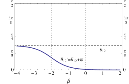
   Figure 19: (a) The dependence of $\overline{\theta}^{\prime}_{12}$ on $\beta=-\log_{\epsilon}(a/|\delta m^{2}_{31}|)$. (b) The $\beta$-dependence of $\overline{\lambda}^{\prime}_{\pm}$.

   Note that in contrast to the neutrino case, $\bar{\theta}^{\prime}_{12}$ decreases monotonically from $\theta_{12}$ to zero as $\beta$ is increased. The $\beta$-dependences of $\overline{s}^{\prime}_{12}=\sin\overline{\theta}^{\prime}_{12}$ and $\overline{c}^{\prime}_{12}=\cos\overline{\theta}^{\prime}_{12}$ are shown in Fig. 20(a). As $\beta$ is increased beyond $\beta=-2$, $\overline{c}^{\prime}_{12}$ grows quickly to one while $\overline{s}^{\prime}_{12}$ damps quickly to zero. The product $\hat{a}\overline{s}^{\prime}_{12}$ stops increasing around $\beta=-2$ and plateau’s to the asymptotic value of $\delta m^{2}_{21}s_{12}c_{12}/c_{13}^{2}=|\delta m^{2}_{31}|O(\epsilon^{2})$ as shown in Fig. 20(b). That is:

   $$\hat{a}\overline{s}^{\prime}_{12} = |\delta m^{2}_{31}|\,O(\epsilon^{-\min(\beta,-2)})\;\leq\;|\delta m^{2}_{31}|\,O(\epsilon^{2})\;,$$ (291)

   $$\hat{a}\overline{c}^{\prime}_{12} = |\delta m^{2}_{31}|\,O(\epsilon^{-\beta})\;.$$ (292)

   Note also that the scales of $\overline{\lambda}^{\prime}_{\pm}$ are given simply by

   $$\overline{\lambda}^{\prime}_{-} = -O(\hat{a})\;=\;-|\delta m^{2}_{31}|\,O(\epsilon^{-\beta})\;,$$ (293)

   $$\overline{\lambda}^{\prime}_{+} = O(\delta m^{2}_{21})\;=\;|\delta m^{2}_{31}|\,O(\epsilon^{2})\;,$$ (294)

   since no level crossing occurs in this case.

   

   

   Figure 20: (a) The $\beta$-dependence of $\overline{s}^{\prime}_{12}=\sin\overline{\theta}^{\prime}_{12}$ and $\overline{c}^{\prime}_{12}=\cos\overline{\theta}^{\prime}_{12}$. (b) The $\beta$-dependence of $a\overline{s}^{\prime}_{12}$ and $a\overline{c}^{\prime}_{12}$. The asymptotic value of $a\overline{s}^{\prime}_{12}$ is $\delta m^{2}_{21}s_{12}c_{12}/c_{13}^{2}\approx 0.014\,|\delta m^{2}_{31}|=O(\varepsilon^{2}|\delta m^{2}_{31}|)$.

2. Second Rotation

   Since $\hat{a}\overline{c}_{12}^{\prime}$ continues to increase with $\beta$ while $\hat{a}\overline{s}_{12}^{\prime}$ does not, we perform a $(1,3)$ rotation on $\overline{H}^{\prime\prime}_{0}$ next.

   Define the matrix $\overline{W}$ as

   $$\overline{W}=\begin{bmatrix}\overline{c}_{\phi}&0&\overline{s}_{\phi}\\ 0&1&0\\ -\overline{s}_{\phi}&0&\overline{c}_{\phi}\end{bmatrix}\;,$$ (295)

   where $\overline{c}_{\phi}=\cos\overline{\phi}$, $\overline{s}_{\phi}=\sin\overline{\phi}$, and

   $$\tan 2\overline{\phi}\;\equiv\;-\dfrac{2\hat{a}\overline{c}_{12}^{\prime}c_{13}s_{13}}{\delta m^{2}_{31}-\hat{a}s_{13}^{2}-\overline{\lambda}^{\prime}_{-}}\;\approx\;-\dfrac{\hat{a}\sin 2\theta_{13}}{(\delta m^{2}_{31}-\delta m^{2}_{21}s_{12}^{2})+\hat{a}\cos 2\theta_{13}}\;.$$ (296)

   The angle $\overline{\phi}$ is in the fourth quadrant when $\delta m^{2}_{31}>0$ (normal hierarchy), and in the first quadrant when $\delta m^{2}_{31}<0$ (inverted hierarchy). The $\beta$-dependence of $\overline{\phi}$ is shown in Fig. 21(a) for both mass hierarchies.

   

   

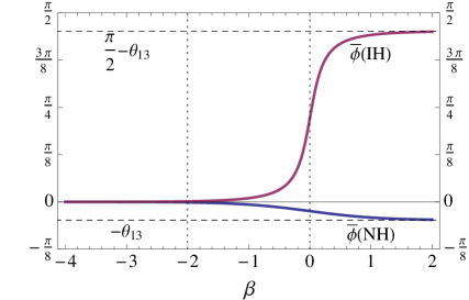
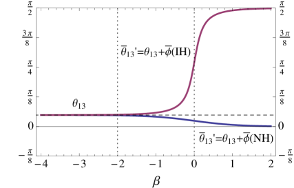
   Figure 21: The dependence of (a) $\overline{\phi}$ and (b) $\overline{\theta}_{13}^{\prime}=\theta_{13}+\overline{\phi}$ on $\beta=-\log_{\,\epsilon}\left(\hat{a}/|\delta m^{2}_{31}|\right)$ for the normal (NH) and inverted (IH) mass hierarchies.

   Using $\overline{W}$, we obtain

   $$\overline{H}_{0}^{\prime\prime\prime} = \overline{W}^{\dagger}\overline{H}_{0}^{\prime\prime}\overline{W}$$ (297)

   $$= \left[\begin{array}[]{ccc}\overline{\lambda}^{\prime\prime}_{\mp}&\hat{a}\overline{s}_{12}^{\prime}c_{13}s_{13}\overline{s}_{\phi}&0\\ \hat{a}\overline{s}_{12}^{\prime}c_{13}s_{13}\overline{s}_{\phi}&\overline{\lambda}^{\prime}_{+}&-\hat{a}\overline{s}_{12}^{\prime}c_{13}s_{13}\overline{c}_{\phi}\\ 0&-\hat{a}\overline{s}_{12}^{\prime}c_{13}s_{13}\overline{c}_{\phi}&\overline{\lambda}^{\prime\prime}_{\pm}\end{array}\right]\;,$$ (301)

   where the upper signs are for the $\delta m^{2}_{31}>0$ case and the lower signs are for the $\delta m^{2}_{31}<0$ case, with

   $$\overline{\lambda}^{\prime\prime}_{\pm}\;\equiv\;\dfrac{[(\delta m^{2}_{31}-\hat{a}s_{13}^{2})+\overline{\lambda}^{\prime}_{-}]\pm\sqrt{[(\delta m^{2}_{31}-\hat{a}s_{13}^{2})-\overline{\lambda}^{\prime}_{-}]^{2}+4(\hat{a}\overline{c}^{\prime}_{12}s_{13}c_{13})^{2}}}{2}\;.$$ (302)

   As $\beta$ is increased beyond 0, the $\overline{\lambda}^{\prime\prime}_{\pm}$ asymptote to

   $$\overline{\lambda}^{\prime\prime}_{+} \rightarrow \delta m^{2}_{31}c_{13}^{2}+\delta m^{2}_{21}s_{12}^{2}s_{13}^{2}\;,$$ (303)

   $$\overline{\lambda}^{\prime\prime}_{-} \rightarrow -\hat{a}+\delta m^{2}_{31}s_{13}^{2}+\delta m^{2}_{21}s_{12}^{2}c_{13}^{2}\;,$$ (304)

   for both mass hierarchies. Note that $\overline{\lambda}^{\prime\prime}_{-}<0<\overline{\lambda}^{\prime\prime}_{+}$ for the $\delta m^{2}_{31}>0$ case, while both $\overline{\lambda}^{\prime\prime}_{\pm}<0$ for the $\delta m^{2}_{31}<0$ case. The $\beta$-dependences of $\overline{\lambda}^{\prime\prime}_{\pm}$ are shown in Fig. 22. Order-of-magnitude-wise, we have

   $$\begin{array}[]{lll}\overline{\lambda}^{\prime\prime}_{-}\;=\;-|\delta m^{2}_{31}|\,O(\epsilon^{-\beta})\;,&\overline{\lambda}^{\prime\prime}_{+}\;=\;\phantom{+}|\delta m^{2}_{31}|\,O(1)\;,&\mbox{if $\delta m^{2}_{31}>0$}\;,\\ \overline{\lambda}^{\prime\prime}_{+}\;=\;-|\delta m^{2}_{31}|\,O(\epsilon^{-\min(\beta,0)})\;,&\overline{\lambda}^{\prime\prime}_{-}\;=\;-|\delta m^{2}_{31}|\,O(\epsilon^{-\max(\beta,0)})\;,&\mbox{if $\delta m^{2}_{31}<0$}\;.\end{array}$$ (305)

   In particular, in the range $\beta\gtrsim 0$, we have

   $$\begin{array}[]{lll}\overline{\lambda}^{\prime\prime}_{-}\;=\;-|\delta m^{2}_{31}|\,O(\epsilon^{-\beta})\;,&\overline{\lambda}^{\prime\prime}_{+}\;=\;\phantom{+}|\delta m^{2}_{31}|\,O(1)\;,&\mbox{if $\delta m^{2}_{31}>0$}\;,\\ \overline{\lambda}^{\prime\prime}_{+}\;=\;-|\delta m^{2}_{31}|\,O(1)\;,&\overline{\lambda}^{\prime\prime}_{-}\;=\;-|\delta m^{2}_{31}|\,O(\epsilon^{-\beta})\;,&\mbox{if $\delta m^{2}_{31}<0$}\;.\end{array}$$ (306)

   For the off-diagonal terms, we have $\hat{a}\overline{s}_{12}^{\prime}=|\delta m^{2}_{31}|O(\epsilon^{2})$, $c_{13}=O(1)$, $s_{13}=O(\epsilon)$, and

   $$\begin{array}[]{lll}\overline{s}_{\phi}=O(\epsilon),&\overline{c}_{\phi}=O(1),&\mbox{if $\delta m^{2}_{31}>0$}\;,\\ \overline{s}_{\phi}=O(1)\;,&\overline{c}_{\phi}=O(\epsilon)\;,&\mbox{if $\delta m^{2}_{31}<0$}\;.\end{array}$$ (307)

   

   

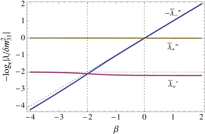
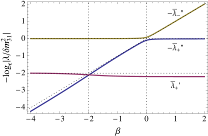
   Figure 22: The $\beta$-dependence of $\overline{\lambda}^{\prime\prime}_{\pm}$ for the (a) normal and (b) inverted mass hierarchies.

   Thus, looking at the elements of $\overline{H}_{0}^{\prime\prime\prime}$ in that range, we find:

   $$\overline{H}_{0}^{\prime\prime\prime}\;=\;|\delta m^{2}_{31}|\begin{bmatrix}O(\epsilon^{-\beta}/1)&O(\epsilon^{4}/\epsilon^{3})&0\\ O(\epsilon^{4}/\epsilon^{3})&O(\epsilon^{2})&O(\epsilon^{3}/\epsilon^{4})\\ 0&O(\epsilon^{3}/\epsilon^{4})&O(1/\epsilon^{-\beta})\end{bmatrix}\;,$$ (308)

   where the elements with two entries denote the two different mass hierarchies, $O(\mathrm{NH}/\mathrm{IH})$, and we see that further diagonalization require angle of order $O(\epsilon^{3})$. Therefore, $\overline{H}_{0}^{\prime\prime\prime}$ is approximately diagonal.

A.2.3 $\eta\neq 0$ Case, Third Rotation

Next, we consider the $\eta\neq 0$ case. Performing the same $(1,2)$ rotation $\overline{V}$ on $\overline{H}_{\eta}^{\prime}=\overline{H}_{0}^{\prime}-\hat{a}\eta\overline{M}_{\eta}^{\prime}$ as we did on $\overline{H}_{0}^{\prime}$, the $\overline{M}_{\eta}^{\prime}$ part is transformed to

$$\overline{V}^{\dagger}\overline{M}_{\eta}^{\prime}(\theta_{12},\theta_{13},\theta_{23},\delta)\overline{V} = \overline{M}_{\eta}^{\prime}(\underbrace{\theta_{12}+\overline{\varphi}}_{\displaystyle=\overline{\theta}_{12}^{\prime}},\theta_{13},\theta_{23},\delta)$$ (309)

$$= \overline{M}_{\eta}^{\prime}(\overline{\theta}_{12}^{\prime},\theta_{13},\theta_{23},\delta)\;.$$ (310)

Using $\overline{\theta}_{12}^{\prime}\rightarrow 0$, $\hat{a}\overline{c}_{12}^{\prime}\rightarrow\hat{a}$, $\hat{a}\overline{s}_{12}^{\prime}\rightarrow O(\epsilon^{2})|\delta m^{2}_{31}|$ as $\beta$ is increased beyond $-2$, we can approximate

$$\hat{a}\eta\overline{M}_{\eta}^{\prime}(\overline{\theta}_{12}^{\prime},\theta_{13},\theta_{23},\delta)$$ (311)

$$\approx \hat{a}\eta\overline{M}_{\eta}^{\prime}(0,\theta_{13},\theta_{23},\delta)$$ (312)

$$= \hat{a}\eta\begin{bmatrix}-s_{13}^{2}\cos(2\theta_{23})&-e^{i\delta}s_{13}\sin(2\theta_{23})&s_{13}c_{13}\cos(2\theta_{23})\\ -e^{-i\delta}s_{13}\sin(2\theta_{23})&\cos(2\theta_{23})&e^{-i\delta}c_{13}\sin(2\theta_{23})\\ s_{13}c_{13}\cos(2\theta_{23})&e^{i\delta}c_{13}\sin(2\theta_{23})&-c_{13}^{2}\cos(2\theta_{23})\end{bmatrix}\;.$$ (313)

Performing the $(1,3)$ rotation $\overline{W}$ next, we find

$$\overline{W}^{\dagger}\overline{M}_{\eta}^{\prime}(0,\theta_{13},\theta_{23},\delta)\overline{W}$$ (314)

$$= \overline{M}_{\eta}^{\prime}(0,\underbrace{\theta_{13}+\overline{\phi}}_{\displaystyle\overline{\theta}_{13}^{\prime}},\theta_{23},\delta)$$ (315)

$$= \overline{M}_{\eta}^{\prime}(0,\overline{\theta}^{\prime}_{13},\theta_{23},\delta)$$ (316)

$$= \begin{bmatrix}-\overline{s}_{13}^{\prime 2}\cos(2\theta_{23})&-e^{i\delta}\overline{s}_{13}^{\prime}\sin(2\theta_{23})&\overline{s}_{13}^{\prime}\overline{c}_{13}^{\prime}\cos(2\theta_{23})\\ -e^{-i\delta}\overline{s}_{13}^{\prime}\sin(2\theta_{23})&\cos(2\theta_{23})&e^{-i\delta}\overline{c}_{13}^{\prime}\sin(2\theta_{23})\\ \overline{s}_{13}^{\prime}\overline{c}_{13}^{\prime}\cos(2\theta_{23})&e^{i\delta}\overline{c}_{13}^{\prime}\sin(2\theta_{23})&-\overline{c}_{13}^{\prime 2}\cos(2\theta_{23})\end{bmatrix}\;,$$ (317)

where $\overline{s}^{\prime}_{13}=\sin\overline{\theta}_{13}^{\prime}$, $\overline{c}^{\prime}_{13}=\cos\overline{\theta}_{13}^{\prime}$. The angle $\overline{\theta}_{13}^{\prime}=\theta_{13}+\overline{\phi}$ can be calculated directly without the need to calculate $\overline{\phi}$ using

$$\tan 2\overline{\theta}_{13}^{\prime}\;=\;\dfrac{(\delta m^{2}_{31}-\delta m^{2}_{21}s_{12}^{2})\sin(2\theta_{13})}{(\delta m^{2}_{31}-\delta m^{2}_{21}s_{12}^{2})\cos(2\theta_{13})+\hat{a}}\;,$$ (318)

and its $\beta$-dependence is shown in Fig. 21(b). In contrast to the neutrino case, $\overline{\theta}_{13}^{\prime}$ increases rapidly to $\pi/2$ when $\delta m^{2}_{31}<0$, while damping to zero when $\delta m^{2}_{31}>0$ once $\beta$ is increased above zero. Consequently, $\hat{a}\cos\overline{\theta}_{13}^{\prime}$ for the $\delta m^{2}_{31}<0$ case, and $\hat{a}\sin\overline{\theta}_{13}^{\prime}$ for the $\delta m^{2}_{31}>0$ case plateau to $c_{13}s_{13}(1-\epsilon^{2}s_{12}^{2})|\delta m^{2}_{31}|=O(\epsilon)|\delta m^{2}_{31}|$ as $\beta$ is increased as shown in Fig. 23. Note that in the $\delta m^{2}_{31}<0$ case, $\hat{a}\cos\overline{\theta}_{13}^{\prime}$ increased to $O(1)|\delta m^{2}_{31}|$ in the vicinity of $\beta=0$ before plateauing to $O(\epsilon)|\delta m^{2}_{31}|$. As in the neutrino case with $\delta m^{2}_{31}>0$, this will cause a slight problem with our approximation later. We now look at the normal and inverted mass hierarchy cases separately.

(a) Normal Hierarchy

(b) Inverted Hierarchy

(c) Normal Hierarchy

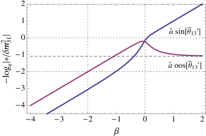
(d) Inverted Hierarchy

Figure 23: The dependence of $\sin\theta^{\prime}_{13}$ and $\cos\theta^{\prime}_{13}$ on $\beta=-\log_{\,\epsilon}\left(\hat{a}/|\delta m^{2}_{31}|\right)$ for the (a) normal and (b) inverted mass hierarchies. The dependence of $\hat{a}\sin\theta^{\prime}_{13}$ and $\hat{a}\cos\theta^{\prime}_{13}$ on $\beta=-\log_{\,\epsilon}\left(\hat{a}/|\delta m^{2}_{31}|\right)$ for the (c) normal and (d) inverted mass hierarchies.

1. $\bm{\delta m^{2}_{31}>}0$ Case

   

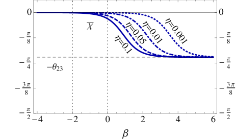
   (a) $\eta>0$

   

   (b) $\eta<0$

   

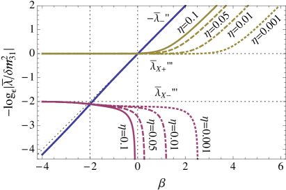
   (c) $\eta>0$

   

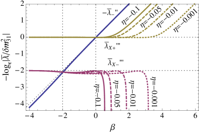
   (d) $\eta<0$

   

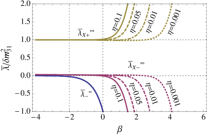
   (e) $\eta>0$

   

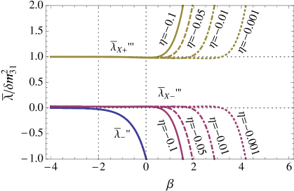
   (f) $\eta<0$

   Figure 24: Normal hierarchy case. The $\beta$-dependence of $\overline{\chi}$ and $\overline{\lambda}^{\prime\prime\prime}_{X\pm}$ for several values of $\eta$ with $s_{23}^{2}=0.4$.

   In the $\delta m^{2}_{31}>0$ case $\hat{a}\overline{s}_{13}^{\prime}\rightarrow O(\epsilon)|\delta m^{2}_{31}|$ as $\beta$ is increased beyond 0. Therefore, we can approximate

   $$H_{\eta}^{\prime\prime\prime} = \overline{W}^{\dagger}\overline{V}^{\dagger}\overline{H}_{\eta}^{\prime}\overline{V}\overline{W}$$ (319)

   $$\approx \overline{H}_{0}^{\prime\prime\prime}-\hat{a}\eta\overline{M}_{\eta}^{\prime}(0,\overline{\theta}_{13}^{\prime},\theta_{23},\delta)$$ (320)

   $$\approx \begin{bmatrix}\overline{\lambda}^{\prime\prime}_{-}&0&0\\ 0&\overline{\lambda}_{+}^{\prime}-\hat{a}\eta\cos(2\theta_{23})&-\hat{a}\eta e^{-i\delta}\overline{c}_{13}^{\prime}\sin(2\theta_{23})\\ 0&-\hat{a}\eta e^{i\delta}\overline{c}_{13}^{\prime}\sin(2\theta_{23})&\overline{\lambda}^{\prime\prime}_{+}+\hat{a}\eta\overline{c}_{13}^{\prime 2}\cos(2\theta_{23})\end{bmatrix}\;,$$ (321)

   where we have dropped off-diagonal terms of order $O(\epsilon^{3})|\delta m^{2}_{31}|$ or smaller. Define the matrix $\overline{X}$ as

   $$\overline{X}\;=\;\begin{bmatrix}1&0&0\\ 0&\overline{c}_{\chi}&\overline{s}_{\chi}e^{-i\delta}\\ 0&-\overline{s}_{\chi}e^{+i\delta}&\overline{c}_{\chi}\end{bmatrix}\;,$$ (322)

   where $\overline{c}_{\chi}=\cos\overline{\chi}$, $\overline{s}_{\chi}=\sin\overline{\chi}$, and

   $$\tan 2\overline{\chi} \equiv \dfrac{-2\hat{a}\eta\overline{c}_{13}^{\prime}\sin(2\theta_{23})}{(\overline{\lambda}^{\prime\prime}_{+}-\overline{\lambda}^{\prime}_{+})+\hat{a}\eta(1+\overline{c}_{13}^{\prime 2})\cos(2\theta_{23})}$$ (323)

   $$\approx -\dfrac{2\hat{a}\eta\sin(2\theta_{23})}{[\delta m^{2}_{31}c_{13}^{2}-\delta m^{2}_{21}(c_{12}^{2}-s_{12}^{2}s_{13}^{2})]+2\hat{a}\eta\cos(2\theta_{23})}\;.$$ (324)

   Note that

   $$-\theta_{23}\;<\;\overline{\chi}\;\leq\;0\quad\mbox{for $\eta>0$}\;,\qquad 0\;\leq\;\overline{\chi}\;<\;\dfrac{\pi}{2}-\theta_{23}\quad\mbox{for $\eta<0$}\;.$$ (325)

   The $\beta$-dependence of $\overline{\chi}$ is shown in Fig. 24 for several values of $\eta$, both positive (Fig. 24(a)) and negative (Fig. 24(b)).

   Using $\overline{X}$, we find

   $$\overline{H}^{\prime\prime\prime\prime}_{\eta+}\;=\;\overline{X}^{\dagger}\overline{H}_{\eta}^{\prime\prime\prime}\overline{X}\;\approx\;\begin{bmatrix}\overline{\lambda}^{\prime\prime}_{-}&0&0\\ 0&\overline{\lambda}^{\prime\prime\prime}_{X-}&0\\ 0&0&\overline{\lambda}^{\prime\prime\prime}_{X+}\end{bmatrix}\;,$$ (326)

   where

   $$\overline{\lambda}^{\prime\prime\prime}_{X\pm}$$ (327)

   $$\equiv \dfrac{(\overline{\lambda}^{\prime\prime}_{+}+\overline{\lambda}^{\prime}_{+}-\hat{a}\eta\overline{s}_{13}^{\prime 2}\cos 2\theta_{23})\pm\sqrt{[\overline{\lambda}^{\prime\prime}_{+}-\overline{\lambda}^{\prime}_{+}+\hat{a}\eta(1+\overline{c}_{13}^{\prime 2})\cos 2\theta_{23}]^{2}+4(\hat{a}\eta\overline{c}_{13}^{\prime}\sin 2\theta_{23})^{2}}}{2}\;.$$ (328)

   Thus, $\overline{H}_{\eta+}^{\prime\prime\prime\prime}$ is approximately diagonal. The asymptotic forms of $\overline{\lambda}_{X\pm}^{\prime\prime\prime}$ at $\beta\gg 0$ are

   $$\overline{\lambda}^{\prime\prime\prime}_{X+} \rightarrow \phantom{-}\hat{a}|\eta|+\left\{\begin{array}[]{ll}\delta m^{2}_{31}c_{13}^{2}c_{23}^{2}+\delta m^{2}_{21}(c_{12}^{2}s_{23}^{2}+s_{12}^{2}s_{13}^{2}c_{23}^{2})&\mbox{for $\eta>0$}\\ \delta m^{2}_{31}c_{13}^{2}s_{23}^{2}+\delta m^{2}_{21}(c_{12}^{2}c_{23}^{2}+s_{12}^{2}s_{13}^{2}s_{23}^{2})&\mbox{for $\eta<0$}\end{array}\right.$$ (332)

   $$\overline{\lambda}^{\prime\prime\prime}_{X-} \rightarrow -\hat{a}|\eta|+\left\{\begin{array}[]{ll}\delta m^{2}_{31}c_{13}^{2}s_{23}^{2}+\delta m^{2}_{21}(c_{12}^{2}c_{23}^{2}+s_{12}^{2}s_{13}^{2}s_{23}^{2})&\mbox{for $\eta>0$}\\ \delta m^{2}_{31}c_{13}^{2}c_{23}^{2}+\delta m^{2}_{21}(c_{12}^{2}s_{23}^{2}+s_{12}^{2}s_{13}^{2}c_{23}^{2})&\mbox{for $\eta<0$}\end{array}\right.$$ (335)

   Note that $\overline{\lambda}^{\prime\prime\prime}_{X\pm}$ have the same asymptotics as $\lambda^{\prime\prime\prime}_{X\pm}$ for the neutrino case except with the $\eta>0$ and $\eta<0$ cases reversed. The $\beta$-dependence of $\overline{\lambda}_{X\pm}^{\prime\prime\prime}$ are shown in Figs. 24(c) to (f).

2. $\bm{\delta m^{2}_{31}<}0$ Case

   

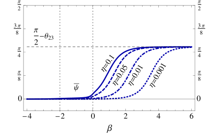
   (a) $\eta>0$

   

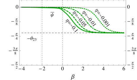
   (b) $\eta<0$

   

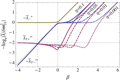
   (c) $\eta>0$

   

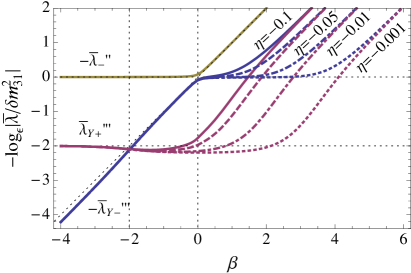
   (d) $\eta<0$

   

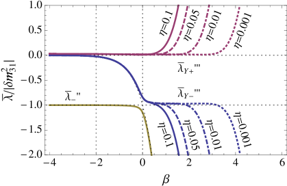
   (e) $\eta>0$

   

   (f) $\eta<0$

   Figure 25: Inverted hierarchy case. The $\beta$-dependence of $\overline{\psi}$ and $\overline{\lambda}^{\prime\prime\prime}_{Y\pm}$ for several values of $\eta$ with $s_{23}^{2}=0.4$.

   In the $\delta m^{2}_{31}<0$ case $\hat{a}\overline{c}_{13}^{\prime}\rightarrow O(\epsilon)|\delta m^{2}_{31}|$ as $\beta$ is increased beyond 0. Therefore, we can approximate

   $$H_{\eta}^{\prime\prime\prime} = \overline{W}^{\dagger}\overline{V}^{\dagger}\overline{H}_{\eta}^{\prime}\overline{V}\overline{W}$$ (336)

   $$\approx \overline{H}_{0}^{\prime\prime\prime}-\hat{a}\eta\overline{M}_{\eta}^{\prime}(0,\overline{\theta}_{13}^{\prime},\theta_{23},\delta)$$ (337)

   $$\approx \begin{bmatrix}\overline{\lambda}^{\prime\prime}_{+}+\hat{a}\eta\overline{s}_{13}^{\prime 2}\cos(2\theta_{23})&\hat{a}\eta e^{i\delta}\overline{s}_{13}^{\prime}\sin(2\theta_{23})&0\\ \hat{a}\eta e^{-i\delta}\overline{s}_{13}^{\prime}\sin(2\theta_{23})&\overline{\lambda}_{+}^{\prime}-\hat{a}\eta\cos(2\theta_{23})&0\\ 0&0&\overline{\lambda}^{\prime\prime}_{-}\end{bmatrix}\;,$$ (338)

   where we have dropped off-diagonal terms of order $O(\epsilon^{3})|\delta m^{2}_{31}|$ or smaller. Define the matrix $\overline{Y}$ as

   $$\overline{Y}=\left[\begin{array}[]{ccc}\overline{c}_{\psi}&\overline{s}_{\psi}e^{+i\delta}&0\\ -\overline{s}_{\psi}e^{-i\delta}&\overline{c}_{\psi}&0\\ 0&0&1\end{array}\right]\;,$$ (339)

   where $\overline{c}_{\psi}=\cos\overline{\psi}$, $\overline{s}_{\psi}=\sin\overline{\psi}$, and

   $$\tan 2\overline{\psi} \equiv -\dfrac{2\hat{a}\eta\overline{s}_{13}^{\prime}\sin(2\theta_{23})}{(\overline{\lambda}^{\prime\prime}_{+}-\overline{\lambda}^{\prime}_{+})+\hat{a}\eta(1+\overline{s}_{13}^{\prime 2})\cos(2\theta_{23})}$$ (340)

   $$\approx -\dfrac{2\hat{a}\eta\sin(2\theta_{23})}{[\delta m^{2}_{31}c_{13}^{2}-\delta m^{2}_{21}(c_{12}^{2}-s_{12}^{2}s_{13}^{2})]+2\hat{a}\eta\cos(2\theta_{23})}\;.$$ (341)

   Note that

   $$0\;\leq\;\overline{\psi}\;<\;\dfrac{\pi}{2}-\theta_{23}\quad\mbox{for $\eta>0$}\;,\qquad-\theta_{23}\;<\;\overline{\psi}\;\leq\;0\quad\mbox{for $\eta<0$}\;.$$ (342)

   The $\beta$-dependence of $\overline{\psi}$ is shown in Fig. 25 for several values of $\eta$, both positive (Fig. 25(a)) and negative (Fig. 25(b)).

   Using $\overline{Y}$, we find

   $$\overline{H}^{\prime\prime\prime\prime}_{\eta-}\;=\;\overline{Y}^{\dagger}\overline{H}_{\eta}^{\prime\prime\prime}\overline{Y}\;\approx\;\left[\begin{array}[]{ccc}\overline{\lambda}^{\prime\prime\prime}_{Y-}&0&0\\ 0&\overline{\lambda}^{\prime\prime\prime}_{Y+}&0\\ 0&0&\overline{\lambda}^{\prime\prime}_{-}\end{array}\right]\;,$$ (343)

   where

   $$\overline{\lambda}^{\prime\prime\prime}_{Y\pm}$$ (344)

   $$\equiv \dfrac{(\overline{\lambda}^{\prime\prime}_{+}+\overline{\lambda}^{\prime}_{+}-\hat{a}\eta\overline{c}_{13}^{\prime 2}\cos 2\theta_{23})\pm\sqrt{[\overline{\lambda}^{\prime\prime}_{+}-\overline{\lambda}^{\prime}_{+}+\hat{a}\eta(1+\overline{s}_{13}^{\prime 2})\cos 2\theta_{23}]^{2}+4(\hat{a}\eta\overline{s}_{13}^{\prime}\sin 2\theta_{23})^{2}}}{2}\;.$$ (345)

   Therefore, $\overline{H}^{\prime\prime\prime\prime}_{\eta-}$ is approximately diagonal. The asymptotic forms of $\overline{\lambda}_{Y\pm}^{\prime\prime\prime}$ at $\beta\gg 0$ are

   $$\overline{\lambda}^{\prime\prime\prime}_{Y+} \rightarrow \phantom{-}\hat{a}|\eta|+\left\{\begin{array}[]{ll}-|\delta m^{2}_{31}|c_{13}^{2}c_{23}^{2}+\delta m^{2}_{21}(c_{12}^{2}s_{23}^{2}+s_{12}^{2}s_{13}^{2}c_{23}^{2})&\mbox{for $\eta>0$}\\ -|\delta m^{2}_{31}|c_{13}^{2}s_{23}^{2}+\delta m^{2}_{21}(c_{12}^{2}c_{23}^{2}+s_{12}^{2}s_{13}^{2}s_{23}^{2})&\mbox{for $\eta<0$}\end{array}\right.$$ (349)

   $$\overline{\lambda}^{\prime\prime\prime}_{Y-} \rightarrow -\hat{a}|\eta|+\left\{\begin{array}[]{ll}-|\delta m^{2}_{31}|c_{13}^{2}s_{23}^{2}+\delta m^{2}_{21}(c_{12}^{2}c_{23}^{2}+s_{12}^{2}s_{13}^{2}s_{23}^{2})&\mbox{for $\eta>0$}\\ -|\delta m^{2}_{31}|c_{13}^{2}c_{23}^{2}+\delta m^{2}_{21}(c_{12}^{2}s_{23}^{2}+s_{12}^{2}s_{13}^{2}c_{23}^{2})&\mbox{for $\eta<0$}\end{array}\right.$$ (352)

   Note that $\overline{\lambda}^{\prime\prime\prime}_{Y\pm}$ have the same asymptotics as $\lambda^{\prime\prime\prime}_{Y\pm}$ for the neutrino case except with the $\eta>0$ and $\eta<0$ cases reversed. The $\beta$-dependence of $\overline{\psi}$ and $\overline{\lambda}^{\prime\prime\prime}_{Y\pm}$ are shown in Fig. 25.

A.3 Effective Mixing Angles for Anti-Neutrinos

We have discovered that the unitary matrix which approximately diagonalizes $\overline{H}$ is $\overset{\lower 1.0pt\hbox{$\scriptstyle{\backsim}$}}{U}{}^{*}=U^{*}Q_{3}^{*}\overline{V}\,\overline{W}\,\overline{X}$ when $\delta m^{2}_{31}>0$, and $\overset{\lower 1.0pt\hbox{$\scriptstyle{\backsim}$}}{U}{}^{*}=U^{*}Q_{3}^{*}\overline{V}\,\overline{W}\,\overline{Y}$ when $\delta m^{2}_{31}<0$. Taking the complex conjugate, these are respectively $\overset{\lower 1.0pt\hbox{$\scriptstyle{\backsim}$}}{U}{}=UQ_{3}\overline{V}\,\overline{W}\,\overline{X}^{*}$ when $\delta m^{2}_{31}>0$, and $\overset{\lower 1.0pt\hbox{$\scriptstyle{\backsim}$}}{U}{}=UQ_{3}\overline{V}\,\overline{W}\,\overline{Y}^{*}$ when $\delta m^{2}_{31}<0$.

In the following, we rewrite the mixing matrix in matter $\overset{\lower 1.0pt\hbox{$\scriptstyle{\backsim}$}}{U}{}$ into the form

$$\overset{\lower 1.0pt\hbox{$\scriptstyle{\backsim}$}}{U}\;=\;R_{23}(\overset{\lower 1.0pt\hbox{$\scriptstyle{\backsim}$}}{\theta}_{23},0)R_{13}(\overset{\lower 1.0pt\hbox{$\scriptstyle{\backsim}$}}{\theta}_{13},\overset{\lower 1.0pt\hbox{$\scriptstyle{\backsim}$}}{\delta})R_{12}(\overset{\lower 1.0pt\hbox{$\scriptstyle{\backsim}$}}{\theta}_{12},0)\;,$$ (353)

absorbing the extra mixing angles and CP phase into appropriate definitions of the ‘running’ parameters $\overset{\lower 1.0pt\hbox{$\scriptstyle{\backsim}$}}{\theta}_{12}$, $\overset{\lower 1.0pt\hbox{$\scriptstyle{\backsim}$}}{\theta}_{13}$, $\overset{\lower 1.0pt\hbox{$\scriptstyle{\backsim}$}}{\theta}_{23}$, and $\overset{\lower 1.0pt\hbox{$\scriptstyle{\backsim}$}}{\delta}$. As in the neutrino case, frequent use is made of Eq. (151).

• $\delta m^{2}_{31}>0$ Case:

  Using Eq. (151), it is straightforward to show that

  $$\overset{\lower 1.0pt\hbox{$\scriptstyle{\backsim}$}}{U} = UQ_{3}\overline{V}\,\overline{W}\,\overline{X}^{*}$$ (354)

  $$= \underbrace{R_{23}(\theta_{23},0)R_{13}(\theta_{13},\delta)R_{12}(\theta_{12},0)}_{\displaystyle U}Q_{3}\underbrace{R_{12}(\overline{\varphi},0)}_{\displaystyle\overline{V}}\underbrace{R_{13}(\overline{\phi},0)}_{\displaystyle\overline{W}}\underbrace{R_{23}(\overline{\chi},-\delta)}_{\displaystyle\overline{X}^{*}}$$ (355)

  $$= R_{23}(\theta_{23},0)Q_{3}R_{13}(\theta_{13},0)R_{12}(\theta_{12},0)R_{12}(\overline{\varphi},0)R_{13}(\overline{\phi},0)R_{23}(\overline{\chi},-\delta)$$ (356)

  $$= R_{23}(\theta_{23},0)Q_{3}R_{13}(\theta_{13},0)R_{12}(\underbrace{\theta_{12}+\overline{\varphi}}_{\displaystyle=\overline{\theta}_{12}^{\prime}},0)R_{13}(\overline{\phi},0)R_{23}(\overline{\chi},-\delta)$$ (357)

  $$= R_{23}(\theta_{23},0)Q_{3}R_{13}(\theta_{13},0)R_{12}(\overline{\theta}_{12}^{\prime},0)R_{13}(\overline{\phi},0)R_{23}(\overline{\chi},-\delta)\;,$$ (358)

  where in the last and penultimate lines we have combined the two $12$-rotations into one. We now commute $R_{13}(\overline{\phi},0)R_{23}(\overline{\chi},\delta)$ through the other mixing matrices to the left as follows:

  • Step 1: Commutation of $R_{13}(\overline{\phi},0)$ through $R_{12}(\overline{\theta}_{12}^{\prime},0)$.

    In the range $\beta\gtrsim 0$, the angle $\theta^{\prime}_{12}$ is approximately equal to zero, so we can approximate

    $$R_{12}(\theta^{\prime}_{12},0)\;\approx\;R_{12}(0,0)\;=\;\begin{bmatrix}1&0&0\\ 0&1&0\\ 0&0&1\end{bmatrix}\;.$$ (359)

    Note that

    $$R_{12}(0,0)R_{13}(\overline{\phi},0)\;=\;R_{13}(\overline{\phi},0)R_{12}(0,0)$$ (360)

    for any $\overline{\phi}$. On the other hand, in the range $\beta\lesssim-1$ the angle $\overline{\phi}$ is negligibly small, so we can approximate

    $$R_{13}(\overline{\phi},0)\;\approx\;R_{13}(0,0)\;=\;\begin{bmatrix}1&0&0\\ 0&1&0\\ 0&0&1\end{bmatrix}\;.$$ (361)

    Note that

    $$R_{12}(\overline{\theta}^{\prime}_{12},0)R_{13}(0,0)\;=\;R_{13}(0,0)R_{12}(\overline{\theta}^{\prime}_{12},0)$$ (362)

    for any $\overline{\theta}^{\prime}_{12}$. Therefore, for all $\beta$ we have

    $$R_{12}(\overline{\theta}^{\prime}_{12},0)R_{13}(\overline{\phi},0)\;\approx\;R_{13}(\overline{\phi},0)R_{12}(\overline{\theta}^{\prime}_{12},0)\;,$$ (363)

    and

    $$\overset{\lower 1.0pt\hbox{$\scriptstyle{\backsim}$}}{U} = R_{23}(\theta_{23},0)Q_{3}R_{13}(\theta_{13},0)R_{12}(\overline{\theta}_{12}^{\prime},0)R_{13}(\overline{\phi},0)R_{23}(\overline{\chi},-\delta)$$ (364)

    $$\approx R_{23}(\theta_{23},0)Q_{3}R_{13}(\theta_{13},0)R_{13}(\overline{\phi},0)R_{12}(\overline{\theta}_{12}^{\prime},0)R_{23}(\overline{\chi},-\delta)$$ (365)

    $$= R_{23}(\theta_{23},0)Q_{3}R_{13}(\underbrace{\theta_{13}+\overline{\phi}}_{\displaystyle=\overline{\theta}^{\prime}_{13}},0)R_{12}(\overline{\theta}_{12}^{\prime},0)R_{23}(\overline{\chi},-\delta)$$ (366)

    $$= R_{23}(\theta_{23},0)Q_{3}R_{13}(\overline{\theta}^{\prime}_{13},0)R_{12}(\overline{\theta}^{\prime}_{12},0)R_{23}(\overline{\chi},-\delta)\;,$$ (367)

    where in the last and penultimate lines we have combined the two $13$-rotations into one. The $\beta$-dependence of $\overline{\theta}^{\prime}_{13}$ was shown in Fig. 21(b).

  • Step 2: Commutation of $R_{23}(\overline{\chi},\delta)$ through $R_{12}(\overline{\theta}_{12}^{\prime},0)$.

    In the range $\beta\gtrsim 0$, the angle $\overline{\theta}^{\prime}_{12}$ is approximately equal to zero as we have noted above and we have the approximation given in Eq. (359). Note that

    $$R_{12}(0,0)R_{23}(\overline{\chi},-\delta)\;=\;R_{23}(\overline{\chi},-\delta)R_{12}(0,0)$$ (368)

    for any $\overline{\chi}$. On the other hand, in the range $\beta\lesssim 0$, the angle $\overline{\chi}$ is negligibly small so we can approximate

    $$R_{23}(\overline{\chi},-\delta)\;\approx\;R_{23}(0,-\delta)\;=\;\begin{bmatrix}1&0&0\\ 0&1&0\\ 0&0&1\end{bmatrix}\;.$$ (369)

    Note that

    $$R_{12}(\overline{\theta}^{\prime}_{12},0)R_{23}(0,\delta)\;=\;R_{23}(0,\delta)R_{12}(\overline{\theta}^{\prime}_{12},0)$$ (370)

    for any $\overline{\theta}^{\prime}_{12}$. Therefore, for all $\beta$ we see that

    $$R_{12}(\overline{\theta}^{\prime}_{12},0)R_{23}(\overline{\chi},-\delta)\;\approx\;R_{23}(\overline{\chi},-\delta)R_{12}(\overline{\theta}^{\prime}_{12},0)\;,$$ (371)

    and

    $$\overset{\lower 1.0pt\hbox{$\scriptstyle{\backsim}$}}{U} \approx R_{23}(\theta_{23},0)Q_{3}R_{13}(\overline{\theta}^{\prime}_{13},0)R_{23}(\overline{\chi},-\delta)R_{12}(\overline{\theta}^{\prime}_{12},0)\;.$$ (372)

  • Step 3: Commutation of $R_{23}(\overline{\chi},-\delta)$ through $R_{13}(\overline{\theta}^{\prime}_{13},0)$.

    When $\delta m^{2}_{31}>0$ we have $\overline{\theta}^{\prime}_{13}\approx 0$ in the range $\beta\gtrsim 1$ so we can approximate

    $$R_{13}(\overline{\theta}^{\prime}_{13},0)\;\approx\;R_{13}(0,0)\;=\;\begin{bmatrix}1&0&0\\ 0&1&0\\ 0&0&1\end{bmatrix}\;.$$ (373)

    Note that

    $$R_{13}(0,0)R_{23}(\overline{\chi},-\delta)\;=\;R_{23}(\overline{\chi},-\delta)R_{13}(0,0)$$ (374)

    for any $\overline{\chi}$. On the other hand, in the range $\beta\lesssim 0$ the angle $\overline{\chi}$ was negligibly small so that we had Eq. (369). Note that

    $$R_{13}(\overline{\theta}^{\prime}_{13},0)R_{12}(0,-\delta)\;=\;R_{23}(0,-\delta)R_{13}(\overline{\theta}^{\prime}_{13},0)\;,$$ (375)

    for any $\overline{\theta}^{\prime}_{13}$. Therefore, for all $\beta$ we see that

    $$R_{13}(\overline{\theta}^{\prime}_{13},0)R_{23}(\overline{\chi},-\delta)\;\approx\;R_{23}(\overline{\chi},-\delta)R_{13}(\overline{\theta}^{\prime}_{13},0)\;,$$ (376)

    and using Eq. (151) we obtain

    $$\overset{\lower 1.0pt\hbox{$\scriptstyle{\backsim}$}}{U} \approx R_{23}(\theta_{23},0)Q_{3}R_{23}(\overline{\chi},-\delta)R_{13}(\overline{\theta}^{\prime}_{13},0)R_{12}(\overline{\theta}^{\prime}_{12},0)$$ (377)

    $$= R_{23}(\theta_{23},0)R_{23}(\overline{\chi},0)R_{13}(\overline{\theta}^{\prime}_{13},\delta)R_{12}(\overline{\theta}^{\prime}_{12},0)Q_{3}$$ (378)

    $$= R_{23}(\underbrace{\theta_{23}+\overline{\chi}}_{\displaystyle=\overline{\theta}^{\prime}_{23}},0)R_{13}(\overline{\theta}^{\prime}_{13},\delta)R_{12}(\overline{\theta}^{\prime}_{12},0)Q_{3}$$ (379)

    $$= R_{23}(\overline{\theta}^{\prime}_{23},0)R_{13}(\overline{\theta}^{\prime}_{13},\delta)R_{12}(\overline{\theta}^{\prime}_{12},0)Q_{3}\;,$$ (380)

    where in the last and penultimate lines we have combined the two $23$-rotations into one. The matrix $Q_{3}$ on the far right can be absorbed into the redefinitions of Majorana phases and can be dropped.

  Thus, we find that the effective mixing matrix $\overset{\lower 1.0pt\hbox{$\scriptstyle{\backsim}$}}{U}$ in the case $\delta m^{2}_{31}>0$ can be expressed as Eq. (353) with the effective mixing angles and effective CP-violating phase given approximately by

  $$\overset{\lower 1.0pt\hbox{$\scriptstyle{\backsim}$}}{\theta}_{12} \approx \overline{\theta}^{\prime}_{12}\;=\;\theta_{12}+\overline{\varphi}\;,$$ (381)

  $$\overset{\lower 1.0pt\hbox{$\scriptstyle{\backsim}$}}{\theta}_{13} \approx \overline{\theta}^{\prime}_{13}\;=\;\theta_{13}+\overline{\phi}\;,$$ (382)

  $$\overset{\lower 1.0pt\hbox{$\scriptstyle{\backsim}$}}{\theta}_{23} \approx \overline{\theta}^{\prime}_{23}\;=\;\theta_{23}+\overline{\chi}\;,$$ (383)

  $$\overset{\lower 1.0pt\hbox{$\scriptstyle{\backsim}$}}{\delta} \approx \delta\;.$$ (384)

• $\delta m^{2}_{31}<0$ Case:

  Using Eq. (151), we obtain

  $$\overset{\lower 1.0pt\hbox{$\scriptstyle{\backsim}$}}{U} = UQ_{3}\overline{V}\,\overline{W}\,\overline{Y}^{*}$$ (385)

  $$= \underbrace{R_{23}(\theta_{23},0)R_{13}(\theta_{13},\delta)R_{12}(\theta_{12},0)}_{\displaystyle U}Q_{3}\underbrace{R_{12}(\overline{\varphi},0)}_{\displaystyle\overline{V}}\underbrace{R_{13}(\overline{\phi},0)}_{\displaystyle\overline{W}}\underbrace{R_{12}(\overline{\psi},\delta)}_{\displaystyle\overline{Y}^{*}}$$ (386)

  $$= R_{23}(\theta_{23},0)Q_{3}R_{13}(\theta_{13},0)R_{12}(\overline{\theta}_{12}^{\prime},0)R_{13}(\overline{\phi},0)R_{12}(\overline{\psi},\delta)\;.$$ (387)

  We now commute $R_{13}(\overline{\phi},0)R_{12}(\overline{\psi},\delta)$ through the other mixing matrices to the left and re-express $\overset{\lower 1.0pt\hbox{$\scriptstyle{\backsim}$}}{U}$ as in Eq. (353), absorbing the extra mixing angles and CP phase into $\overset{\lower 1.0pt\hbox{$\scriptstyle{\backsim}$}}{\theta}_{12}$, $\overset{\lower 1.0pt\hbox{$\scriptstyle{\backsim}$}}{\theta}_{13}$, $\overset{\lower 1.0pt\hbox{$\scriptstyle{\backsim}$}}{\theta}_{23}$, and $\overset{\lower 1.0pt\hbox{$\scriptstyle{\backsim}$}}{\delta}$. The first step is the same as the $\delta m^{2}_{31}>0$ case, the only difference being the $\beta$-dependence of $\overline{\theta}^{\prime}_{13}$, which is also shown in Fig. 21(b).

  • Step 2: Commutation of $R_{12}(\overline{\psi},\delta)$ through $R_{12}(\overline{\theta}_{12}^{\prime},0)$.

    In the range $\beta\gtrsim 0$ the angle $\overline{\theta}^{\prime}_{12}$ is approximately equal to zero as we have noted previously, and we have the approximation given in Eq. (359). Note that

    $$R_{12}(0,0)R_{12}(\overline{\psi},\delta)\;=\;R_{12}(\overline{\psi},\delta)R_{12}(0,0)$$ (388)

    for any $\overline{\psi}$. On the other hand, in the range $\beta\lesssim 0$ the angle $\overline{\psi}$ is negligibly small so that

    $$R_{12}(\overline{\psi},\delta)\;\approx\;R_{12}(0,\delta)\;=\;\begin{bmatrix}1&0&0\\ 0&1&0\\ 0&0&1\end{bmatrix}\;.$$ (389)

    Note that

    $$R_{12}(\overline{\theta}^{\prime}_{12},0)R_{12}(0,\delta)\;=\;R_{12}(0,\delta)R_{12}(\overline{\theta}^{\prime}_{12},0)$$ (390)

    for any $\overline{\theta}^{\prime}_{12}$. Therefore, for all $\beta$ we see that

    $$R_{12}(\overline{\theta}^{\prime}_{12},0)R_{12}(\overline{\psi},\delta)\;\approx\;R_{12}(\overline{\psi},\delta)R_{12}(\overline{\theta}^{\prime}_{12},0)\;,$$ (391)

    and

    $$\overset{\lower 1.0pt\hbox{$\scriptstyle{\backsim}$}}{U}\;\approx\;R_{23}(\theta_{23},0)Q_{3}R_{13}(\overline{\theta}^{\prime}_{13},0)R_{12}(\overline{\psi},\delta)R_{12}(\overline{\theta}^{\prime}_{12},0)\;.$$ (392)

  • Step 3: Commutation of $R_{12}(\overline{\psi},\delta)$ through $R_{13}(\overline{\theta}^{\prime}_{13},0)$.

    When $\delta m^{2}_{31}<0$ we have $\overline{\theta}^{\prime}_{13}\approx\frac{\pi}{2}$ in the range $\beta\gtrsim 1$ so that

    $$R_{13}(\theta^{\prime}_{13},0)\;\approx\;R_{13}\left(\frac{\pi}{2},0\right)\;=\;\begin{bmatrix}0&0&1\\ 0&1&0\\ -1&0&0\end{bmatrix}\;.$$ (393)

    Note that

    $$R_{13}\left(\frac{\pi}{2},0\right)R_{12}(\overline{\psi},\delta)\;=\;R_{23}(\overline{\psi},-\delta)R_{13}\left(\frac{\pi}{2},0\right)$$ (394)

    for all $\overline{\psi}$. On the other hand, in the range $\beta\lesssim 0$ the angle $\overline{\psi}$ was negligibly small so that we had the approximation Eq. (187). Note that

    $$R_{13}(\overline{\theta}^{\prime}_{13},0)R_{12}(0,\delta)\;=\;R_{23}(0,-\delta)R_{13}(\overline{\theta}^{\prime}_{13},0)$$ (395)

    for all $\overline{\theta}^{\prime}_{13}$. Therefore, for all $\beta$ we see that

    $$R_{13}(\overline{\theta}^{\prime}_{13},0)R_{12}(\overline{\psi},\delta)\;\approx\;R_{23}(\overline{\psi},-\delta)R_{13}(\overline{\theta}^{\prime}_{13},0)\;,$$ (396)

    and using Eq. (151) we obtain

    $$\overset{\lower 1.0pt\hbox{$\scriptstyle{\backsim}$}}{U} \approx R_{23}(\theta_{23},0)Q_{3}R_{23}(\overline{\psi},-\delta)R_{13}(\overline{\theta}^{\prime}_{13},0)R_{12}(\overline{\theta}^{\prime}_{12},0)$$ (397)

    $$= R_{23}(\theta_{23},0)R_{23}(\overline{\psi},0)R_{13}(\overline{\theta}^{\prime}_{13},\delta)R_{12}(\overline{\theta}^{\prime}_{12},0)Q_{3}$$ (398)

    $$= R_{23}(\underbrace{\theta_{23}+\overline{\psi}}_{\displaystyle=\overline{\theta}^{\prime}_{23}},0)R_{13}(\overline{\theta}^{\prime}_{13},\delta)R_{12}(\overline{\theta}^{\prime}_{12},0)Q_{3}$$ (399)

    $$= R_{23}(\overline{\theta}^{\prime}_{23},0)R_{13}(\overline{\theta}^{\prime}_{13},\delta)R_{12}(\overline{\theta}^{\prime}_{12},0)Q_{3}\;,$$ (400)

    where in the last and penultimate lines we have combined the two $23$-rotations into one. The matrix $Q_{3}$ on the far right can be absorbed into redefinitions of the Majorana phases and can be dropped.

  Thus, we find that the effective mixing matrix $\overset{\lower 1.0pt\hbox{$\scriptstyle{\backsim}$}}{U}$ for anti-neutrinos in the case $\delta m^{2}_{31}<0$ can be expressed as Eq. (353) with the effective mixing angles and effective CP-violating phase given approximately by

  $$\overset{\lower 1.0pt\hbox{$\scriptstyle{\backsim}$}}{\theta}_{12} \approx \overline{\theta}^{\prime}_{12}\;=\;\theta_{12}+\overline{\varphi}\;,$$ (401)

  $$\overset{\lower 1.0pt\hbox{$\scriptstyle{\backsim}$}}{\theta}_{13} \approx \overline{\theta}^{\prime}_{13}\;=\;\theta_{13}+\overline{\phi}\;,$$ (402)

  $$\overset{\lower 1.0pt\hbox{$\scriptstyle{\backsim}$}}{\theta}_{23} \approx \overline{\theta}^{\prime}_{23}\;=\;\theta_{23}+\overline{\psi}\;,$$ (403)

  $$\overset{\lower 1.0pt\hbox{$\scriptstyle{\backsim}$}}{\delta} \approx \delta\;.$$ (404)

A.4 Summary of Anti-Neutrino Case

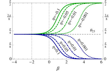
(a) Normal Hierarchy

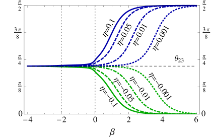
(b) Inverted Hierarchy

Figure 26: The $\beta$-dependence of $\overline{\theta}_{23}^{\prime}$ for the (a) normal and (b) inverted hierarchies for several values of $\eta$ with $s_{23}^{2}=0.4$.

To summarize what we have learned, the inclusion of the $\hat{a}\eta M_{\eta}$ term in the effective Hamiltonian shifts $\theta_{23}$ to $\overline{\theta}_{23}^{\prime}=\theta_{23}+\overline{\chi}$ for the $\delta m^{2}_{31}>0$ case, and to $\overline{\theta}_{23}^{\prime}=\theta_{23}+\overline{\psi}$ for the $\delta m^{2}_{31}<0$ case. For both cases, $\theta_{23}^{\prime}$ can be calculated directly without calculating $\overline{\chi}$ or $\overline{\psi}$ first via the expression

$$\tan 2\overline{\theta}_{23}^{\prime}\;\approx\;\dfrac{[\delta m^{2}_{31}c_{13}^{2}-\delta m^{2}_{21}(c_{12}^{2}-s_{12}^{2}s_{13}^{2})]\sin 2\theta_{23}}{[\delta m^{2}_{31}c_{13}^{2}-\delta m^{2}_{21}(c_{12}^{2}-s_{12}^{2}s_{13}^{2})]\cos 2\theta_{23}+2\hat{a}\eta}\;.$$ (405)

Note that as $\beta$ is increased, $\overline{\theta}_{23}^{\prime}$ runs toward $\dfrac{\pi}{2}$ if $\delta m^{2}_{31}\eta<0$, while it runs toward $0$ if $\delta m^{2}_{31}\eta>0$. The $\beta$-dependence of $\overline{\theta}_{23}^{\prime}$ is shown in Fig. 26. The CP-violating phase $\delta$ remains unaffected and maintains its vacuum value.

The running of the effective mass-squared differences are also modified in the range $\beta\gtrsim 0$. For the $\delta m^{2}_{31}>0$ case, $\overline{\lambda}_{2}$ and $\overline{\lambda}_{3}$ show extra running, while for the $\delta m^{2}_{31}<0$ case, it is $\overline{\lambda}_{1}$ and $\overline{\lambda}_{2}$ that show extra running, cf. Figs. 24 and 25.

A.5 Discussion at the Probability Level

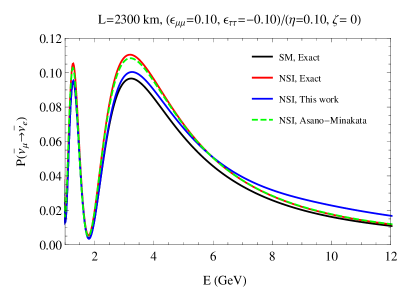
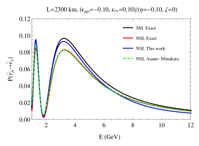
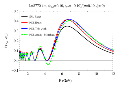
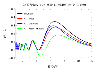
Figure 27: $\bar{\nu}_{\mu}\rightarrow\bar{\nu}_{e}$ transition probability as a function of anti-neutrino energy $E$ in GeV for 2300 km (8770 km) baseline in upper (lower) panels. We compare the analytical expressions of this work and Asano-Minakata Asano:2011nj against the exact numerical result assuming $\eta=0.1,\zeta=0$ (left panels) and $\eta=-0.1,\zeta=0$ (right panels). The solid black curves portray the standard three-flavor oscillation probabilities in matter without NSI’s. In all the panels, we consider $\theta_{23}=40^{\circ})$, $\delta=0^{\circ}$, and inverted mass hierarchy.

Now, we demonstrate how these lepton-flavor-conserving NSI parameters affect the anti-neutrino oscillation probability for the various appearance and the disappearance channels. In Fig. 27, we compare our approximate $\bar{\nu}_{\mu}\rightarrow\bar{\nu}_{e}$ oscillation probabilities (blue curves) as a function of the neutrino energy against the exact numerical results (red curves) assuming $\eta=0.1,\zeta=0$ (left panels) and $\eta=-0.1,\zeta=0$ (right panels). The upper (lower) panels are drawn for 2300 km (8770 km) baseline. Here, in all the panels, we assume $\theta_{23}=40^{\circ}$, $\delta=0^{\circ}$, and inverted mass hierarchy ($\delta m^{2}_{31}<0$). We also compare our results with the approximate expressions of Asano and Minakata Asano:2011nj (dashed green curves).

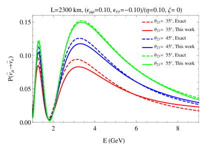
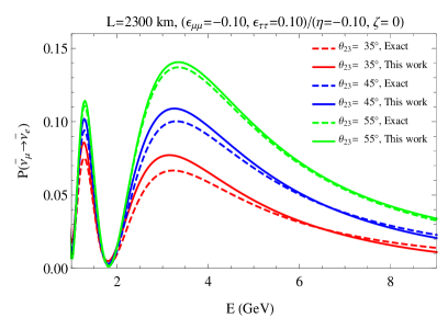
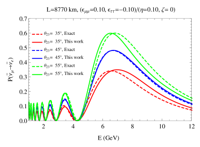
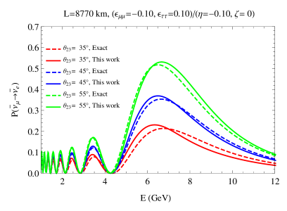
Figure 28: Comparison of our analytical expressions (solid curves) to the exact numerical results (dashed curves) in case of anti-neutrino for various values of $\theta_{23}$. We assume $\delta=0^{\circ}$ and $\delta m^{2}_{31}<0$. Upper (lower) panels are for 2300 km (8770 km) baseline.

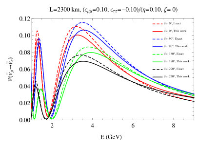
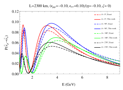
Figure 29: Comparison of our analytical expressions (solid curves) to the exact numerical results (dashed curves) in case of anti-neutrino for different values of the CP-violating phase $\delta$ at 2300 km. To generate these plots, we consider $\theta_{23}=40^{\circ}$ and $\delta m^{2}_{31}<0$.

The accuracy of our analytical approximations as compared to the exact numerical results for different values of $\theta_{23}$ is shown in Fig. 28. All the plots in Fig. 28 have been generated assuming $\delta=0^{\circ}$ and inverted mass hierarchy ($\delta m^{2}_{31}<0$). We take the same choices of $\eta$ and $\zeta$ like in Fig. 27 and results are given for 2300 km (upper panels) and 8770 km (lower panels) baselines. We find that our approximation provides satisfactory match with exact numerical results for different values of $\theta_{23}$. Fig. 29 presents a comparison of our approximate probability expressions (solid curves) against the exact numerical results (dashed curves) assuming four different values of the CP-violating phase $\delta$ at 2300 km. Here, we take $\theta_{23}=40^{\circ}$ and $\delta m^{2}_{31}<0$.

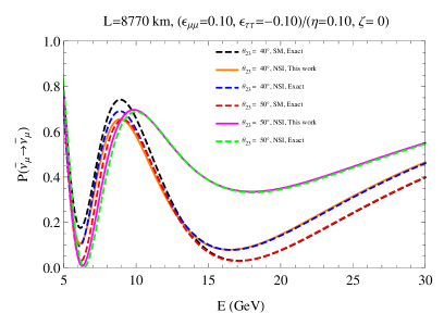
(a) $\eta=0.1,\zeta=0$

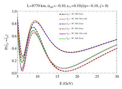
(b) $\eta=-0.1,\zeta=0$

Figure 30: $\bar{\nu}_{\mu}\rightarrow\bar{\nu}_{\mu}$ survival probability as a function of anti-neutrino energy $E$ in GeV for two different values of $\theta_{23}$ at 8770 km baseline. Comparison between the analytical and numerical results assuming $\eta=0.1,\zeta=0$ (left panel) and $\eta=-0.1,\zeta=0$ (right panel). The standard three-flavor oscillation probabilities in matter without NSI’s are also shown. In both the panels, we assume $\delta=0^{\circ}$ and $\delta m^{2}_{31}<0$.

In Fig. 30, we depict the $\bar{\nu}_{\mu}\rightarrow\bar{\nu}_{\mu}$ survival probability in the presence of NSI for two different values of $\theta_{23}$ (40^∘ and 50^∘) at 8770 km baseline. We present the matching between the analytical and numerical results assuming $\eta=0.1,\zeta=0$ (left panel) and $\eta=-0.1,\zeta=0$ (right panel). In both the panels, we consider $\delta=0^{\circ}$ and $\delta m^{2}_{31}<0$. Fig. 30 portrays that our approximate expressions match quite nicely with the numerical results.

Appendix B Comparing Probabilities with Constant & Varying Earth Density Profile

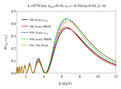
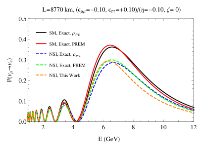
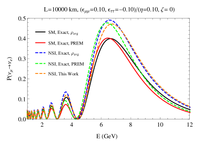
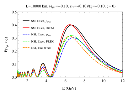
Figure 31: $\nu_{\mu}\rightarrow\nu_{e}$ transition probability as a function of neutrino energy $E$ in GeV for 8770 km (10000 km) baseline in upper (lower) panels. We compare the exact numerical probabilities considering the constant (denoted by ‘$\rho_{\rm avg}$’), and varying (labelled by ‘PREM’) Earth density profiles for both the SM and NSI cases. We also plot our approximate analytical expressions in the presence of NSI. For the NSI’s, we take $\eta=0.1,\zeta=0$ (left panels), and $\eta=-0.1,\zeta=0$ (right panels). In all the panels, we consider $\theta_{23}=40^{\circ}$, $\delta=0^{\circ}$, and normal mass hierarchy.

So far, we considered the line-averaged constant Earth matter density for a given baseline which has been estimated using the PREM profile to present our results. Now, it would be quite interesting to study how the exact numerical probabilities would be affected if we consider the more realistic varying Earth density profile instead of the line-averaged constant matter density for the baselines as large as 8770 km and 10000 km. In Fig. 31, we show the exact numerical probabilities considering the constant and varying Earth density profiles for 8700 km (upper panels) and 10000 km (lower panels) baselines. In the figure legends, the line-averaged constant matter density cases are denoted by ‘$\rho_{\rm avg}$’ and the varying Earth density cases are labelled by ‘PREM’. We perform these comparisons for both the SM and NSI scenarios. For the NSI’s, we take $\eta=0.1,\zeta=0$ (left panels), and $\eta=-0.1,\zeta=0$ (right panels). For the sake of completeness, we also plot the approximate probability expressions in the presence of NSI that we derived in this paper assuming the line-averaged constant Earth matter density based on the PREM profile. Fig. 31 clearly shows that though the line-averaged constant matter density probability does not completely overlap with the PREM-based varying matter density profile probability, it is still fairly accurate. Moreover, the effect due to the inclusion of flavor-diagonal NSI’s is correctly captured in our approximate analytical expressions.

References

- (1) Daya Bay Collaboration, F. An et al., A new measurement of antineutrino oscillation with the full detector configuration at Daya Bay, arXiv:1505.03456.
- (2) Daya Bay Collaboration, F. An et al., Spectral measurement of electron antineutrino oscillation amplitude and frequency at Daya Bay, Phys.Rev.Lett. 112 (2014) 061801, [arXiv:1310.6732].
- (3) Daya Bay Collaboration, F. An et al., Improved Measurement of Electron Antineutrino Disappearance at Daya Bay, Chin. Phys. C37 (2013) 011001, [arXiv:1210.6327].
- (4) RENO Collaboration, J. Ahn et al., Observation of Reactor Electron Antineutrino Disappearance in the RENO Experiment, Phys.Rev.Lett. 108 (2012) 191802, [arXiv:1204.0626].
- (5) Double Chooz Collaboration, Y. Abe et al., Indication for the disappearance of reactor electron antineutrinos in the Double Chooz experiment, Phys.Rev.Lett. 108 (2012) 131801, [arXiv:1112.6353].
- (6) Double Chooz Collaboration, Y. Abe et al., Reactor electron antineutrino disappearance in the Double Chooz experiment, Phys.Rev. D86 (2012) 052008, [arXiv:1207.6632].
- (7) Double Chooz Collaboration, Y. Abe et al., First Measurement of from Delayed Neutron Capture on Hydrogen in the Double Chooz Experiment, Phys.Lett. B723 (2013) 66–70, [arXiv:1301.2948].
- (8) MINOS Collaboration, P. Adamson et al., Electron neutrino and antineutrino appearance in the full MINOS data sample, Phys.Rev.Lett. (2013) [arXiv:1301.4581].
- (9) T2K Collaboration, K. Abe et al., Observation of Electron Neutrino Appearance in a Muon Neutrino Beam, Phys.Rev.Lett. 112 (2014) 061802, [arXiv:1311.4750].
- (10) T2K Collaboration, K. Abe et al., Evidence of Electron Neutrino Appearance in a Muon Neutrino Beam, Phys.Rev. D88 (2013) 032002, [arXiv:1304.0841].
- (11) T2K Collaboration, K. Abe et al., Measurements of neutrino oscillation in appearance and disappearance channels by the T2K experiment with 6.6×10²⁰ protons on target, Phys.Rev. D91 (2015) 072010, [arXiv:1502.01550].
- (12) CHOOZ Collaboration, M. Apollonio et al., Limits on neutrino oscillations from the CHOOZ experiment, Phys.Lett. B466 (1999) 415–430, [hep-ex/9907037].
- (13) Palo Verde Collaboration, A. Piepke, Final results from the Palo Verde neutrino oscillation experiment, Prog.Part.Nucl.Phys. 48 (2002) 113–121.
- (14) Particle Data Group Collaboration, K. Olive et al., Review of Particle Physics, Chin.Phys. C38 (2014) 090001.
- (15) J. Hewett, H. Weerts, R. Brock, J. Butler, B. Casey, et al., Fundamental Physics at the Intensity Frontier, arXiv:1205.2671.
- (16) M. Gonzalez-Garcia, M. Maltoni, and T. Schwetz, Updated fit to three neutrino mixing: status of leptonic CP violation, JHEP 1411 (2014) 052, [arXiv:1409.5439].
- (17) F. Capozzi, G. Fogli, E. Lisi, A. Marrone, D. Montanino, et al., Status of three-neutrino oscillation parameters, circa 2013, Phys.Rev. D89 (2014) 093018, [arXiv:1312.2878].
- (18) D. Forero, M. Tortola, and J. Valle, Neutrino oscillations refitted, Phys.Rev. D90 (2014) 093006, [arXiv:1405.7540].
- (19) K. Abazajian, M. Acero, S. Agarwalla, A. Aguilar-Arevalo, C. Albright, et al., Light Sterile Neutrinos: A White Paper, arXiv:1204.5379.
- (20) M. Blennow and A. Y. Smirnov, Neutrino propagation in matter, Adv.High Energy Phys. 2013 (2013) 972485, [arXiv:1306.2903].
- (21) L. Wolfenstein, Neutrino Oscillations in Matter, Phys.Rev. D17 (1978) 2369–2374.
- (22) S. Mikheev and A. Y. Smirnov, Resonance Amplification of Oscillations in Matter and Spectroscopy of Solar Neutrinos, Sov.J.Nucl.Phys. 42 (1985) 913–917.
- (23) S. Mikheev and A. Y. Smirnov, Resonant amplification of neutrino oscillations in matter and solar neutrino spectroscopy, Nuovo Cim. C9 (1986) 17–26.
- (24) S. K. Agarwalla, Physics Potential of Long-Baseline Experiments, Adv.High Energy Phys. 2014 (2014) 457803, [arXiv:1401.4705].
- (25) S. Pascoli and T. Schwetz, Prospects for neutrino oscillation physics, Adv.High Energy Phys. 2013 (2013) 503401.
- (26) G. Feldman, J. Hartnell, and T. Kobayashi, Long-baseline neutrino oscillation experiments, Adv.High Energy Phys. 2013 (2013) 475749, [arXiv:1210.1778].
- (27) R. Wendell and K. Okumura, Recent progress and future prospects with atmospheric neutrinos, New J.Phys. 17 (2015), no. 2 025006.
- (28) ICAL Collaboration, S. Ahmed et al., Physics Potential of the ICAL detector at the India-based Neutrino Observatory (INO), arXiv:1505.07380.
- (29) M. M. Devi, T. Thakore, S. K. Agarwalla, and A. Dighe, Enhancing sensitivity to neutrino parameters at INO combining muon and hadron information, JHEP 1410 (2014) 189, [arXiv:1406.3689].
- (30) IceCube PINGU Collaboration, M. Aartsen et al., Letter of Intent: The Precision IceCube Next Generation Upgrade (PINGU), arXiv:1401.2046.
- (31) G. L. Fogli and E. Lisi, Tests of three flavor mixing in long baseline neutrino oscillation experiments, Phys.Rev. D54 (1996) 3667–3670, [hep-ph/9604415].
- (32) S. K. Agarwalla, S. Prakash, and S. Uma Sankar, Exploring the three flavor effects with future superbeams using liquid argon detectors, JHEP 1403 (2014) 087, [arXiv:1304.3251].
- (33) H. Minakata, Phenomenology of future neutrino experiments with large Theta(13), Nucl.Phys.Proc.Suppl. 235-236 (2013) 173–179, [arXiv:1209.1690].
- (34) J. Valle, Resonant Oscillations of Massless Neutrinos in Matter, Phys.Lett. B199 (1987) 432.
- (35) M. Guzzo, A. Masiero, and S. Petcov, On the MSW effect with massless neutrinos and no mixing in the vacuum, Phys.Lett. B260 (1991) 154–160.
- (36) E. Roulet, MSW effect with flavor changing neutrino interactions, Phys.Rev. D44 (1991) 935–938.
- (37) Y. Grossman, Nonstandard neutrino interactions and neutrino oscillation experiments, Phys.Lett. B359 (1995) 141–147, [hep-ph/9507344].
- (38) T. Ohlsson, Status of non-standard neutrino interactions, Rept.Prog.Phys. 76 (2013) 044201, [arXiv:1209.2710].
- (39) O. Miranda and H. Nunokawa, Non standard neutrino interactions, arXiv:1505.06254.
- (40) P. Minkowski, at a Rate of One Out of Muon Decays?, Phys.Lett. B67 (1977) 421–428.
- (41) T. Yanagida, HORIZONTAL SYMMETRY AND MASSES OF NEUTRINOS, Conf.Proc. C7902131 (1979) 95–99.
- (42) R. N. Mohapatra and G. Senjanovic, Neutrino Mass and Spontaneous Parity Violation, Phys.Rev.Lett. 44 (1980) 912.
- (43) M. Gell-Mann, P. Ramond, and R. Slansky, Complex Spinors and Unified Theories, Conf.Proc. C790927 (1979) 315–321, [arXiv:1306.4669].
- (44) J. Schechter and J. Valle, Neutrino Masses in Theories, Phys.Rev. D22 (1980) 2227.
- (45) G. Lazarides, Q. Shafi, and C. Wetterich, Proton Lifetime and Fermion Masses in an SO(10) Model, Nucl.Phys. B181 (1981) 287–300.
- (46) R. Mohapatra and J. Valle, Neutrino Mass and Baryon Number Nonconservation in Superstring Models, Phys.Rev. D34 (1986) 1642.
- (47) E. K. Akhmedov, M. Lindner, E. Schnapka, and J. Valle, Left-right symmetry breaking in NJL approach, Phys.Lett. B368 (1996) 270–280, [hep-ph/9507275].
- (48) E. K. Akhmedov, M. Lindner, E. Schnapka, and J. Valle, Dynamical left-right symmetry breaking, Phys.Rev. D53 (1996) 2752–2780, [hep-ph/9509255].
- (49) P. B. Dev and R. Mohapatra, TeV Scale Inverse Seesaw in SO(10) and Leptonic Non-Unitarity Effects, Phys.Rev. D81 (2010) 013001, [arXiv:0910.3924].
- (50) S. M. Boucenna, S. Morisi, and J. W. Valle, The low-scale approach to neutrino masses, Adv.High Energy Phys. 2014 (2014) 831598, [arXiv:1404.3751].
- (51) T. Cheng and L.-F. Li, Neutrino Masses, Mixings and Oscillations in SU(2) x U(1) Models of Electroweak Interactions, Phys.Rev. D22 (1980) 2860.
- (52) A. Zee, A Theory of Lepton Number Violation, Neutrino Majorana Mass, and Oscillation, Phys.Lett. B93 (1980) 389.
- (53) K. Babu, Model of ’Calculable’ Majorana Neutrino Masses, Phys.Lett. B203 (1988) 132.
- (54) M. A. Diaz, J. C. Romao, and J. Valle, Minimal supergravity with R-parity breaking, Nucl.Phys. B524 (1998) 23–40, [hep-ph/9706315].
- (55) M. Hirsch, M. Diaz, W. Porod, J. Romao, and J. Valle, Neutrino masses and mixings from supersymmetry with bilinear R parity violation: A Theory for solar and atmospheric neutrino oscillations, Phys.Rev. D62 (2000) 113008, [hep-ph/0004115].
- (56) V. D. Barger, K. Whisnant, S. Pakvasa, and R. Phillips, Matter Effects on Three-Neutrino Oscillations, Phys.Rev. D22 (1980) 2718.
- (57) H. Zaglauer and K. Schwarzer, The Mixing Angles in Matter for Three Generations of Neutrinos and the MSW Mechanism, Z. Phys. C40 (1988) 273.
- (58) K. Kimura, A. Takamura, and H. Yokomakura, Exact formula of probability and CP violation for neutrino oscillations in matter, Phys.Lett. B537 (2002) 86–94, [hep-ph/0203099].
- (59) K. Kimura, A. Takamura, and H. Yokomakura, Exact formulas and simple CP dependence of neutrino oscillation probabilities in matter with constant density, Phys.Rev. D66 (2002) 073005, [hep-ph/0205295].
- (60) S. Petcov and S. Toshev, Three Neutrino Oscillations in Matter: Analytical Results in the Adiabatic Approximation, Phys.Lett. B187 (1987) 120.
- (61) C. Kim and W. Sze, Adiabatic Resonant Oscillations of Solar Neutrinos in Three Generations, Phys.Rev. D35 (1987) 1404.
- (62) J. Arafune and J. Sato, CP and T violation test in neutrino oscillation, Phys.Rev. D55 (1997) 1653–1658, [hep-ph/9607437].
- (63) J. Arafune, M. Koike, and J. Sato, CP violation and matter effect in long baseline neutrino oscillation experiments, Phys.Rev. D56 (1997) 3093–3099, [hep-ph/9703351]. [Erratum-ibid. D60 (1999) 119905].
- (64) T. Ohlsson and H. Snellman, Three flavor neutrino oscillations in matter, J.Math.Phys. 41 (2000) 2768–2788, [hep-ph/9910546]. [Erratum-ibid. 42 (2001) 2345].
- (65) M. Freund, Analytic approximations for three neutrino oscillation parameters and probabilities in matter, Phys.Rev. D64 (2001) 053003, [hep-ph/0103300].
- (66) A. Cervera, A. Donini, M. Gavela, J. Gomez Cadenas, P. Hernandez, et al., Golden measurements at a neutrino factory, Nucl.Phys. B579 (2000) 17–55, [hep-ph/0002108]. Erratum: Nucl. Phys. B593 (2001) 731-732.
- (67) E. K. Akhmedov, R. Johansson, M. Lindner, T. Ohlsson, and T. Schwetz, Series expansions for three flavor neutrino oscillation probabilities in matter, JHEP 0404 (2004) 078, [hep-ph/0402175].
- (68) M. Honda, Y. Kao, N. Okamura, and T. Takeuchi, A Simple parameterization of matter effects on neutrino oscillations, hep-ph/0602115.
- (69) K. Asano and H. Minakata, Large-Theta(13) Perturbation Theory of Neutrino Oscillation for Long-Baseline Experiments, JHEP 1106 (2011) 022, [arXiv:1103.4387].
- (70) S. K. Agarwalla, Y. Kao, and T. Takeuchi, Analytical approximation of the neutrino oscillation matter effects at large , JHEP 1404 (2014) 047, [arXiv:1302.6773].
- (71) H. Minakata and S. J. Parke, Simple and Compact Expressions for Neutrino Oscillation Probabilities in Matter, arXiv:1505.01826.
- (72) C. G. J. Jacobi, Über ein leichtes Verfahren, die in der Theorie der Säkularstörangen vorkommenden Gleichungen numerisch Aufzuloösen, Crelle’s Journal 30 (1846) 51–94.
- (73) S. K. Agarwalla, Y. Kao, C. Sun, and T. Takeuchi, Running of Neutrino Oscillation Parameters in Matter in the presence of Flavor-Non-Diagonal Non-Standard Interactions of the Neutrino, . In preparation.
- (74) M. Gonzalez-Garcia, Y. Grossman, A. Gusso, and Y. Nir, New CP violation in neutrino oscillations, Phys.Rev. D64 (2001) 096006, [hep-ph/0105159].
- (75) T. Ota, J. Sato, and N.-a. Yamashita, Oscillation enhanced search for new interaction with neutrinos, Phys.Rev. D65 (2002) 093015, [hep-ph/0112329].
- (76) O. Yasuda, On the exact formula for neutrino oscillation probability by Kimura, Takamura and Yokomakura, arXiv:0704.1531.
- (77) J. Kopp, M. Lindner, T. Ota, and J. Sato, Non-standard neutrino interactions in reactor and superbeam experiments, Phys.Rev. D77 (2008) 013007, [arXiv:0708.0152].
- (78) N. Ribeiro, H. Minakata, H. Nunokawa, S. Uchinami, and R. Zukanovich-Funchal, Probing Non-Standard Neutrino Interactions with Neutrino Factories, JHEP 0712 (2007) 002, [arXiv:0709.1980].
- (79) M. Blennow and T. Ohlsson, Approximative two-flavor framework for neutrino oscillations with non-standard interactions, Phys.Rev. D78 (2008) 093002, [arXiv:0805.2301].
- (80) T. Kikuchi, H. Minakata, and S. Uchinami, Perturbation Theory of Neutrino Oscillation with Nonstandard Neutrino Interactions, JHEP 0903 (2009) 114, [arXiv:0809.3312].
- (81) D. Meloni, T. Ohlsson, and H. Zhang, Exact and Approximate Formulas for Neutrino Mixing and Oscillations with Non-Standard Interactions, JHEP 0904 (2009) 033, [arXiv:0901.1784].
- (82) M. Honda, N. Okamura, and T. Takeuchi, Matter Effect on Neutrino Oscillations from the violation of Universality in Neutrino Neutral Current Interactions, hep-ph/0603268.
- (83) M. Honda, Y. Kao, N. Okamura, A. Pronin, and T. Takeuchi, Constraints on New Physics from Matter Effects on Neutrino Oscillation, hep-ph/0610281.
- (84) M. Honda, Y. Kao, N. Okamura, A. Pronin, and T. Takeuchi, The Effect of Topcolor Assisted Technicolor, and other models, on Neutrino Oscillation, arXiv:0704.0369.
- (85) M. Honda, Y. Kao, N. Okamura, A. Pronin, and T. Takeuchi, Constraints on New Physics from Long Baseline Neutrino Oscillation Experiments, arXiv:0707.4545.
- (86) S. Antusch, J. P. Baumann, and E. Fernandez-Martinez, Non-Standard Neutrino Interactions with Matter from Physics Beyond the Standard Model, Nucl.Phys. B810 (2009) 369–388, [arXiv:0807.1003].
- (87) W. Loinaz and T. Takeuchi, Constraints on topcolor assisted technicolor models from vertex corrections, Phys.Rev. D60 (1999) 015005, [hep-ph/9812377].
- (88) O. Lebedev, W. Loinaz, and T. Takeuchi, Constraints on R-parity violating couplings from lepton universality, Phys.Rev. D61 (2000) 115005, [hep-ph/9910435].
- (89) L. N. Chang, O. Lebedev, W. Loinaz, and T. Takeuchi, Constraints on gauged and related theories, Phys.Rev. D63 (2001) 074013, [hep-ph/0010118].
- (90) S. Antusch, C. Biggio, E. Fernandez-Martinez, M. Gavela, and J. Lopez-Pavon, Unitarity of the Leptonic Mixing Matrix, JHEP 0610 (2006) 084, [hep-ph/0607020].
- (91) X. He, G. C. Joshi, H. Lew, and R. Volkas, NEW Z-prime PHENOMENOLOGY, Phys.Rev. D43 (1991) 22–24.
- (92) X.-G. He, G. C. Joshi, H. Lew, and R. Volkas, Simplest Z-prime model, Phys.Rev. D44 (1991) 2118–2132.
- (93) E. Ma, Gauged and radiative neutrino masses, Phys.Lett. B433 (1998) 74–81, [hep-ph/9709474].
- (94) E. Ma and D. Roy, Phenomenology of the gauge boson, Phys.Rev. D58 (1998) 095005, [hep-ph/9806210].
- (95) E. Ma and U. Sarkar, Gauged and baryogenesis, Phys.Lett. B439 (1998) 95–102, [hep-ph/9807307].
- (96) E. Ma, D. Roy, and U. Sarkar, A Seesaw model for atmospheric and solar neutrino oscillations, Phys.Lett. B444 (1998) 391–396, [hep-ph/9810309].
- (97) E. Ma and D. Roy, Minimal seesaw model for atmospheric and solar neutrino oscillations, Phys.Rev. D59 (1999) 097702, [hep-ph/9811266].
- (98) C. T. Hill, Topcolor assisted technicolor, Phys.Lett. B345 (1995) 483–489, [hep-ph/9411426].
- (99) W. Buchmuller and D. Wyler, Constraints on SU(5) Type Leptoquarks, Phys.Lett. B177 (1986) 377.
- (100) W. Buchmuller, R. Ruckl, and D. Wyler, Leptoquarks in Lepton - Quark Collisions, Phys.Lett. B191 (1987) 442–448.
- (101) M. Leurer, A Comprehensive study of leptoquark bounds, Phys.Rev. D49 (1994) 333–342, [hep-ph/9309266].
- (102) S. Davidson, D. C. Bailey, and B. A. Campbell, Model independent constraints on leptoquarks from rare processes, Z.Phys. C61 (1994) 613–644, [hep-ph/9309310].
- (103) J. L. Hewett and T. G. Rizzo, Much ado about leptoquarks: A Comprehensive analysis, Phys.Rev. D56 (1997) 5709–5724, [hep-ph/9703337].
- (104) F. Cuypers and S. Davidson, Bileptons: Present limits and future prospects, Eur.Phys.J. C2 (1998) 503–528, [hep-ph/9609487].
- (105) S. Dimopoulos and L. Susskind, Mass Without Scalars, Nucl.Phys. B155 (1979) 237–252.
- (106) E. Eichten and K. D. Lane, Dynamical Breaking of Weak Interaction Symmetries, Phys.Lett. B90 (1980) 125–130.
- (107) S. Dimopoulos and J. R. Ellis, Challenges for Extended Technicolor Theories, Nucl.Phys. B182 (1982) 505–528.
- (108) V. D. Barger, G. Giudice, and T. Han, Some New Aspects of Supersymmetry R-Parity Violating Interactions, Phys.Rev. D40 (1989) 2987.
- (109) H. K. Dreiner, An Introduction to explicit R-parity violation, Adv.Ser.Direct.High Energy Phys. 21 (2010) 565–583, [hep-ph/9707435].
- (110) R. Barbier, C. Berat, M. Besancon, M. Chemtob, A. Deandrea, et al., R-parity violating supersymmetry, Phys.Rept. 420 (2005) 1–202, [hep-ph/0406039].
- (111) O. Lebedev, W. Loinaz, and T. Takeuchi, Constraints on R-parity violating couplings from LEP / SLD hadronic observables, Phys.Rev. D62 (2000) 015003, [hep-ph/9911479].
- (112) A. Zee, Quantum Numbers of Majorana Neutrino Masses, Nucl.Phys. B264 (1986) 99.
- (113) T. Ohlsson, T. Schwetz, and H. Zhang, Non-standard neutrino interactions in the Zee-Babu model, Phys.Lett. B681 (2009) 269–275, [arXiv:0909.0455].
- (114) Y. Chikashige, R. N. Mohapatra, and R. Peccei, Are There Real Goldstone Bosons Associated with Broken Lepton Number?, Phys.Lett. B98 (1981) 265.
- (115) J. Schechter and J. Valle, Neutrino Decay and Spontaneous Violation of Lepton Number, Phys.Rev. D25 (1982) 774.
- (116) M. Fukugita and T. Yanagida, Neutrino Oscillation in Matter Induced by Charged Scalar Particles, Phys.Lett. B206 (1988) 93.
- (117) M. S. Bilenky and A. Santamaria, One loop effective Lagrangian for a standard model with a heavy charged scalar singlet, Nucl.Phys. B420 (1994) 47–93, [hep-ph/9310302].
- (118) G. Gelmini and M. Roncadelli, Left-Handed Neutrino Mass Scale and Spontaneously Broken Lepton Number, Phys.Lett. B99 (1981) 411.
- (119) M. Malinsky, T. Ohlsson, and H. Zhang, Non-Standard Neutrino Interactions from a Triplet Seesaw Model, Phys.Rev. D79 (2009) 011301, [arXiv:0811.3346].
- (120) P. Langacker and D. London, Lepton Number Violation and Massless Nonorthogonal Neutrinos, Phys.Rev. D38 (1988) 907.
- (121) S. M. Bilenky and C. Giunti, Seesaw type mixing and muon-neutrino —¿ tau-neutrino oscillations, Phys.Lett. B300 (1993) 137–140, [hep-ph/9211269].
- (122) E. Nardi, E. Roulet, and D. Tommasini, Limits on neutrino mixing with new heavy particles, Phys.Lett. B327 (1994) 319–326, [hep-ph/9402224].
- (123) D. Tommasini, G. Barenboim, J. Bernabeu, and C. Jarlskog, Nondecoupling of heavy neutrinos and lepton flavor violation, Nucl.Phys. B444 (1995) 451–467, [hep-ph/9503228].
- (124) S. Bergmann and A. Kagan, Z - induced FCNCs and their effects on neutrino oscillations, Nucl.Phys. B538 (1999) 368–386, [hep-ph/9803305].
- (125) M. Czakon, J. Gluza, and M. Zralek, Nonunitary neutrino mixing matrix and CP violating neutrino oscillations, Acta Phys.Polon. B32 (2001) 3735–3744, [hep-ph/0109245].
- (126) N. Fornengo, M. Maltoni, R. Tomas, and J. Valle, Probing neutrino nonstandard interactions with atmospheric neutrino data, Phys.Rev. D65 (2002) 013010, [hep-ph/0108043].
- (127) B. Bekman, J. Gluza, J. Holeczek, J. Syska, and M. Zralek, Matter effects and CP violating neutrino oscillations with nondecoupling heavy neutrinos, Phys.Rev. D66 (2002) 093004, [hep-ph/0207015].
- (128) W. Loinaz, N. Okamura, T. Takeuchi, and L. Wijewardhana, The NuTeV anomaly, neutrino mixing, and a heavy Higgs boson, Phys.Rev. D67 (2003) 073012, [hep-ph/0210193].
- (129) W. Loinaz, N. Okamura, S. Rayyan, T. Takeuchi, and L. Wijewardhana, Quark lepton unification and lepton flavor nonconservation from a TeV scale seesaw neutrino mass texture, Phys.Rev. D68 (2003) 073001, [hep-ph/0304004].
- (130) W. Loinaz, N. Okamura, S. Rayyan, T. Takeuchi, and L. Wijewardhana, The NuTeV anomaly, lepton universality, and nonuniversal neutrino gauge couplings, Phys.Rev. D70 (2004) 113004, [hep-ph/0403306].
- (131) V. Barger, S. Geer, and K. Whisnant, Neutral currents and tests of three-neutrino unitarity in long-baseline experiments, New J.Phys. 6 (2004) 135, [hep-ph/0407140].
- (132) M. Malinsky, T. Ohlsson, Z.-z. Xing, and H. Zhang, Non-unitary neutrino mixing and CP violation in the minimal inverse seesaw model, Phys.Lett. B679 (2009) 242–248, [arXiv:0905.2889].
- (133) M. Malinsky, T. Ohlsson, and H. Zhang, Non-unitarity effects in a realistic low-scale seesaw model, Phys.Rev. D79 (2009) 073009, [arXiv:0903.1961].
- (134) F. Escrihuela, D. Forero, O. Miranda, M. Tortola, and J. Valle, On the description of non-unitary neutrino mixing, arXiv:1503.08879.
- (135) M. Gavela, D. Hernandez, T. Ota, and W. Winter, Large gauge invariant non-standard neutrino interactions, Phys.Rev. D79 (2009) 013007, [arXiv:0809.3451].
- (136) B. Pontecorvo, Inverse beta-processes and non-conservation of lepton charge, Sov. Phys. JETP 7 (1958) 172–173.
- (137) Z. Maki, M. Nakagawa, and S. Sakata, Remarks on the unified model of elementary particles, Prog. Theor. Phys. 28 (1962) 870–880.
- (138) B. Pontecorvo, Neutrino Experiments and the Problem of Conservation of Leptonic Charge, Sov. Phys. JETP 26 (1968) 984–988.
- (139) R. Allen, H. Chen, P. Doe, R. Hausammann, W. Lee, et al., Study of electron-neutrino electron elastic scattering at LAMPF, Phys.Rev. D47 (1993) 11–28.
- (140) LSND Collaboration, L. Auerbach et al., Measurement of electron - neutrino - electron elastic scattering, Phys.Rev. D63 (2001) 112001, [hep-ex/0101039].
- (141) F. Reines, H. Gurr, and H. Sobel, Detection of Scattering, Phys.Rev.Lett. 37 (1976) 315–318.
- (142) G. Vidyakin, V. Vyrodov, I. Gurevich, Y. Kozlov, V. Martemyanov, et al., Limitations on the magnetic moment and charge radius of the electron-anti-neutrino, JETP Lett. 55 (1992) 206–210.
- (143) A. Derbin, A. Chernyi, L. Popeko, V. Muratova, G. Shishkina, et al., Experiment on anti-neutrino scattering by electrons at a reactor of the Rovno nuclear power plant, JETP Lett. 57 (1993) 768–772.
- (144) MUNU Collaboration, Z. Daraktchieva et al., Limits on the neutrino magnetic moment from the MUNU experiment, Phys.Lett. B564 (2003) 190–198, [hep-ex/0304011].
- (145) TEXONO Collaboration, M. Deniz et al., Measurement of Nu(e)-bar -Electron Scattering Cross-Section with a CsI(Tl) Scintillating Crystal Array at the Kuo-Sheng Nuclear Power Reactor, Phys.Rev. D81 (2010) 072001, [arXiv:0911.1597].
- (146) CHARM Collaboration, J. Dorenbosch et al., Experimental Verification of the Universality of and Coupling to the Neutral Weak Current, Phys.Lett. B180 (1986) 303.
- (147) CHARM-II Collaboration, P. Vilain et al., Flavor universality of neutrino couplings with the Z, Phys.Lett. B320 (1994) 203–205.
- (148) CHARM-II Collaboration, P. Vilain et al., Precision measurement of electroweak parameters from the scattering of muon-neutrinos on electrons, Phys.Lett. B335 (1994) 246–252.
- (149) NuTeV Collaboration, G. Zeller et al., A Precise determination of electroweak parameters in neutrino nucleon scattering, Phys.Rev.Lett. 88 (2002) 091802, [hep-ex/0110059].
- (150) NNPDF Collaboration, R. D. Ball et al., Precision determination of electroweak parameters and the strange content of the proton from neutrino deep-inelastic scattering, Nucl.Phys. B823 (2009) 195–233, [arXiv:0906.1958].
- (151) W. Bentz, I. Cloet, J. Londergan, and A. Thomas, Reassessment of the NuTeV determination of the weak mixing angle, Phys.Lett. B693 (2010) 462–466, [arXiv:0908.3198].
- (152) ALEPH Collaboration, R. Barate et al., Searches for supersymmetry in the photon(s) plus missing energy channels at -GeV and 172-GeV, Phys.Lett. B420 (1998) 127–139, [hep-ex/9710009].
- (153) ALEPH Collaboration, R. Barate et al., Single photon and multiphoton production in collisions at a center-of-mass energy of 183-GeV, Phys.Lett. B429 (1998) 201–214.
- (154) ALEPH Collaboration, A. Heister et al., Single photon and multiphoton production in collisions at up to 209-GeV, Eur.Phys.J. C28 (2003) 1–13.
- (155) L3 Collaboration, M. Acciarri et al., Single and multiphoton events with missing energy in collisions at -GeV -GeV, Phys.Lett. B415 (1997) 299–310.
- (156) L3 Collaboration, M. Acciarri et al., Single and multiphoton events with missing energy in collisions at -GeV, Phys.Lett. B444 (1998) 503–515.
- (157) L3 Collaboration, M. Acciarri et al., Single and multiphoton events with missing energy in collisions at -GeV, Phys.Lett. B470 (1999) 268–280, [hep-ex/9910009].
- (158) OPAL Collaboration, K. Ackerstaff et al., Photonic events with large missing energy in collisions at -GeV, Phys.Lett. B391 (1997) 210–220.
- (159) OPAL Collaboration, K. Ackerstaff et al., Search for anomalous production of photonic events with missing energy in collisions at -GeV to 172-GeV, Eur.Phys.J. C2 (1998) 607–625, [hep-ex/9801024].
- (160) OPALx Collaboration, G. Abbiendi et al., Search for anomalous photonic events with missing energy in collisions at -GeV, 136-GeV and 183-GeV, Eur.Phys.J. C8 (1999) 23–40, [hep-ex/9810021].
- (161) OPAL Collaboration, G. Abbiendi et al., Photonic events with missing energy in collisions at -GeV, Eur.Phys.J. C18 (2000) 253–272, [hep-ex/0005002].
- (162) DELPHI Collaboration, J. Abdallah et al., Photon events with missing energy in collisions at -GeV to 209-GeV, Eur.Phys.J. C38 (2005) 395–411, [hep-ex/0406019].
- (163) Super-Kamiokande Collaboration, G. Mitsuka et al., Study of Non-Standard Neutrino Interactions with Atmospheric Neutrino Data in Super-Kamiokande I and II, Phys.Rev. D84 (2011) 113008, [arXiv:1109.1889].
- (164) IceCube Collaboration, A. Gross, Atmospheric Neutrino Oscillations in IceCube, Nucl.Phys.Proc.Suppl. 237-238 (2013) 272–274, [arXiv:1301.4339].
- (165) IceCube Collaboration, R. Abbasi et al., The Design and Performance of IceCube DeepCore, Astropart.Phys. 35 (2012) 615–624, [arXiv:1109.6096].
- (166) KamLAND Collaboration, S. Abe et al., Precision Measurement of Neutrino Oscillation Parameters with KamLAND, Phys.Rev.Lett. 100 (2008) 221803, [arXiv:0801.4589].
- (167) SNO Collaboration, B. Aharmim et al., An Independent Measurement of the Total Active B-8 Solar Neutrino Flux Using an Array of He-3 Proportional Counters at the Sudbury Neutrino Observatory, Phys.Rev.Lett. 101 (2008) 111301, [arXiv:0806.0989].
- (168) Borexino Collaboration, C. Arpesella et al., Direct Measurement of the Be-7 Solar Neutrino Flux with 192 Days of Borexino Data, Phys.Rev.Lett. 101 (2008) 091302, [arXiv:0805.3843].
- (169) Borexino Collaboration, G. Bellini, J. Benziger, D. Bick, S. Bonetti, G. Bonfini, et al., Precision measurement of the 7Be solar neutrino interaction rate in Borexino, Phys.Rev.Lett. 107 (2011) 141302, [arXiv:1104.1816].
- (170) Z. Berezhiani and A. Rossi, Limits on the nonstandard interactions of neutrinos from colliders, Phys.Lett. B535 (2002) 207–218, [hep-ph/0111137].
- (171) Z. Berezhiani, R. Raghavan, and A. Rossi, Probing nonstandard couplings of neutrinos at the Borexino detector, Nucl.Phys. B638 (2002) 62–80, [hep-ph/0111138].
- (172) M. Hirsch, E. Nardi, and D. Restrepo, Bounds on the tau and muon neutrino vector and axial vector charge radius, Phys.Rev. D67 (2003) 033005, [hep-ph/0210137].
- (173) S. Davidson, C. Pena-Garay, N. Rius, and A. Santamaria, Present and future bounds on nonstandard neutrino interactions, JHEP 0303 (2003) 011, [hep-ph/0302093].
- (174) M. Maltoni, Standard and nonstandard physics in neutrino oscillations, Nucl.Phys.Proc.Suppl. 114 (2003) 191–196, [hep-ph/0210111].
- (175) A. Friedland, C. Lunardini, and C. Pena-Garay, Solar neutrinos as probes of neutrino matter interactions, Phys.Lett. B594 (2004) 347, [hep-ph/0402266].
- (176) A. Friedland, C. Lunardini, and M. Maltoni, Atmospheric neutrinos as probes of neutrino-matter interactions, Phys.Rev. D70 (2004) 111301, [hep-ph/0408264].
- (177) A. Friedland and C. Lunardini, A Test of tau neutrino interactions with atmospheric neutrinos and K2K, Phys.Rev. D72 (2005) 053009, [hep-ph/0506143].
- (178) J. Barranco, O. Miranda, C. Moura, and J. Valle, Constraining non-standard interactions in nu(e) e or anti-nu(e) e scattering, Phys.Rev. D73 (2006) 113001, [hep-ph/0512195].
- (179) J. Barranco, O. Miranda, C. Moura, and J. Valle, Constraining non-standard neutrino-electron interactions, Phys.Rev. D77 (2008) 093014, [arXiv:0711.0698].
- (180) A. Bolanos, O. Miranda, A. Palazzo, M. Tortola, and J. Valle, Probing non-standard neutrino-electron interactions with solar and reactor neutrinos, Phys.Rev. D79 (2009) 113012, [arXiv:0812.4417].
- (181) F. Escrihuela, O. Miranda, M. Tortola, and J. Valle, Constraining nonstandard neutrino-quark interactions with solar, reactor and accelerator data, Phys.Rev. D80 (2009) 105009, [arXiv:0907.2630].
- (182) C. Biggio, M. Blennow, and E. Fernandez-Martinez, Loop bounds on non-standard neutrino interactions, JHEP 0903 (2009) 139, [arXiv:0902.0607].
- (183) C. Biggio, M. Blennow, and E. Fernandez-Martinez, General bounds on non-standard neutrino interactions, JHEP 0908 (2009) 090, [arXiv:0907.0097].
- (184) D. Forero and M. Guzzo, Constraining nonstandard neutrino interactions with electrons, Phys.Rev. D84 (2011) 013002.
- (185) F. Escrihuela, M. Tortola, J. Valle, and O. Miranda, Global constraints on muon-neutrino non-standard interactions, Phys.Rev. D83 (2011) 093002, [arXiv:1103.1366].
- (186) S. K. Agarwalla, F. Lombardi, and T. Takeuchi, Constraining Non-Standard Interactions of the Neutrino with Borexino, JHEP 1212 (2012) 079, [arXiv:1207.3492].
- (187) A. Esmaili and A. Y. Smirnov, Probing Non-Standard Interaction of Neutrinos with IceCube and DeepCore, JHEP 1306 (2013) 026, [arXiv:1304.1042].
- (188) A. N. Khan, D. W. McKay, and F. Tahir, Sensitivity of medium-baseline reactor neutrino mass-hierarchy experiments to nonstandard interactions, Phys.Rev. D88 (2013) 113006, [arXiv:1305.4350].
- (189) A. N. Khan, D. W. McKay, and F. Tahir, Short baseline reactor scattering experiments and nonstandard neutrino interactions at source and detector, Phys.Rev. D90 (2014) 053008, [arXiv:1407.4263].
- (190) I. Girardi and D. Meloni, Constraining new physics scenarios in neutrino oscillations from Daya Bay data, Phys. Rev. D90 (2014), no. 7 073011, [arXiv:1403.5507].
- (191) I. Girardi, D. Meloni, and S. T. Petcov, The Daya Bay and T2K results on and Non-Standard Neutrino Interactions, Nucl. Phys. B886 (2014) 31–42, [arXiv:1405.0416].
- (192) S. K. Agarwalla, P. Bagchi, D. V. Forero, and M. Tortola, Probing Non-Standard Interactions at Daya Bay, arXiv:1412.1064.
- (193) M. Gonzalez-Garcia, M. Maltoni, and J. Salvado, Testing matter effects in propagation of atmospheric and long-baseline neutrinos, JHEP 1105 (2011) 075, [arXiv:1103.4365].
- (194) M. Gonzalez-Garcia, M. Maltoni, J. Salvado, and T. Schwetz, Global fit to three neutrino mixing: critical look at present precision, arXiv:1209.3023v.
- (195) A. M. Dziewonski and D. L. Anderson, Preliminary reference earth model, Physics of the Earth and Planetary Interiors 25 (1981) 297–356.
- (196) S. K. Agarwalla, T. Li, and A. Rubbia, An Incremental approach to unravel the neutrino mass hierarchy and CP violation with a long-baseline Superbeam for large , JHEP 1205 (2012) 154, [arXiv:1109.6526].
- (197) A. Stahl, C. Wiebusch, A. Guler, M. Kamiscioglu, R. Sever, et al., Expression of Interest for a very long baseline neutrino oscillation experiment (LBNO), CERN-SPSC-2012-021, SPSC-EOI-007.
- (198) LAGUNA-LBNO Collaboration, S. Agarwalla et al., Optimised sensitivity to leptonic CP violation from spectral information: the LBNO case at 2300 km baseline, arXiv:1412.0593.
- (199) S. K. Agarwalla and P. Hernandez, Probing the Neutrino Mass Hierarchy with Super-Kamiokande, JHEP 1210 (2012) 086, [arXiv:1204.4217].
- (200) H. Minakata, Large-Theta(13) Perturbation Theory of Neutrino Oscillation, Acta Phys.Polon. B40 (2009) 3023–3031, [arXiv:0910.5545].
- (201) Z. Rahman, A. Dasgupta, and R. Adhikari, The Discovery reach of violation in neutrino oscillation with non-standard interaction effects, J.Phys. G42 (2015), no. 6 065001, [arXiv:1503.03248].
- (202) J. Kopp, T. Ota, and W. Winter, Neutrino factory optimization for non-standard interactions, Phys.Rev. D78 (2008) 053007, [arXiv:0804.2261].
- (203) P. Coloma, A. Donini, J. Lopez-Pavon, and H. Minakata, Non-Standard Interactions at a Neutrino Factory: Correlations and CP violation, JHEP 1108 (2011) 036, [arXiv:1105.5936].
- (204) A. Chatterjee, P. Mehta, D. Choudhury, and R. Gandhi, Testing non-standard neutrino matter interactions in atmospheric neutrino propagation, arXiv:1409.8472.
- (205) I. Mocioiu and W. Wright, Non-standard neutrino interactions in the mu-tau sector, Nucl.Phys. B893 (2015) 376–390, [arXiv:1410.6193].
- (206) S. Choubey and T. Ohlsson, Bounds on Non-Standard Neutrino Interactions Using PINGU, Phys.Lett. B739 (2014) 357–364, [arXiv:1410.0410].
- (207) S. K. Agarwalla, S. Choubey, S. Goswami, and A. Raychaudhuri, Neutrino parameters from matter effects in P(ee) at long baselines, Phys.Rev. D75 (2007) 097302, [hep-ph/0611233].
- (208) C. Jarlskog, Commutator of the Quark Mass Matrices in the Standard Electroweak Model and a Measure of Maximal CP Violation, Phys.Rev.Lett. 55 (1985) 1039.
- (209) A. Khatun, S. S. Chatterjee, T. Thakore, and S. K. Agarwalla, Enhancing Sensitivity to Non-Standard Neutrino Interactions at INO combining muon and hadron information, . In preparation.