On the Approximation Theory of Linear Variational Subspace Design

Abstract

Solving large-scale optimization on-the-fly is often a difficult task for real-time computer graphics applications. To tackle this challenge, model reduction is a well-adopted technique. Despite its usefulness, model reduction often requires a handcrafted subspace that spans a domain that hypothetically embodies desirable solutions. For many applications, obtaining such subspaces case-by-case either is impossible or requires extensive human labors, hence does not readily have a scalable solution for growing number of tasks. We propose linear variational subspace design for large-scale constrained quadratic programming, which can be computed automatically without any human interventions. We provide meaningful approximation error bound that substantiates the quality of calculated subspace, and demonstrate its empirical success in interactive deformable modeling for triangular and tetrahedral meshes.

I.3.5Computer GraphicsComputational Geometry and Object Modeling I.3.6Computer GraphicsMethodology and TechniquesInteraction techniques

1 Introduction

In computer graphics realm, solving optimization with a substantially large amount of variables is often an expensive task. In order to speed up the computations, model reduction has been introduced as a useful technique, particularly for interactive and real-time applications. In solving a large-scale optimization problem, it typically assumes that a desired solution approximately lies in a manifold of much lower dimension that is independent of the variable size. Therefore, it is possible to cut down calculations to a computationally practical level by only exploring variability (i.e., different solutions subject to different constraints) in a suitably chosen low-order space, meanwhile, attempting to produce visually convincing results just-in-time. In this paper, we re-examine model reduction techniques for quadratic optimization with uncertain linear constraints, which has been widely used in interactively modeling deformable surfaces and solids.

Modeling deformable meshes has been an established topic in computer graphics for years [Sorkine et al. 2004, Yu et al. 2004]. Mesh deformation of high quality is accessible via off-line solving a large-scale optimization whose variables are in complexity of mesh nodes. A studio work-flow in mesh deformable modeling often involves trial-and-error loops: an artist tries different sets of constraints and explores for desirable poses. In such processes, an interactive technique helps to save the computation time where approximate solutions are firstly displayed for the purpose of guidance before a final solution is calculated and exported. Nevertheless, interactive techniques related to real-time mesh modeling has been less successful than their off-line siblings till today. Existing work based on model reduction often requires a high quality subspace as the input, which typically demands human interventions in constructing them. Exemplars include cage-based deformations [Huang et al. 2006, Ben-Chen et al. 2009], LBS with additional weights [Jacobson et al. 2012], LBS with skeletons [Shi et al. 2007], and LBS with point/region handles [Au et al. 2007, Sumner et al. 2007]. The time spent on constructing such reduced models is as much as, if not more than, that spent on on-site modeling. In industrial deployments, companies have to hire many artists with expertise skills for rigging a large set of models before those models are used in productions. This poses the necessity for a fully automatic subspace generation method. This problems have received attentions in the past. For example, data-driven methods have been developed for deformable meshes, where a learning algorithm tries to capture the characteristics of deformable mesh sequences and applies to a different task [Sumner et al. 2005, Der et al. 2006]. However, they still struggle to face two challenges: 1) Scalability: Like approaches relying on human inputs, obtaining a deformable sequence of scanned meshes can also be expensive. No words to say if we want to build a deformable mesh database containing large number of models with heterogeneous shapes. 2) Applicability: Many models of complex geometries or topologies are relatively difficult to rig, and there are no easy ways to build a set of controllers with skinning weights to produce desirable deformations. Though we see there have been several workarounds for a domain specific mesh sets, such as faces and clothes, an automatically computed subspace for arbitrary meshes, which is cheaply obtained, still can be beneficial, if not all, for fast prototyping or exploratory purposes: the set of constraints chosen on-site is exported for computing a deformation with full quality in the off-line stage.

In this paper, we introduce an automatic and principled way to create reduced models, which might be applied to other computationally intensive optimization scenarios other than mesh deformation. Our main idea is very simple: in solving a constrained quadratic programming, we observe that Karush-Kuhn-Tucker (KKT) condition implicitly defines an effective subspace that can be directly reused for on-site subsequent optimization. We name this linear variational subspace (for short, variational subspace). Our contribution is to theoretically study the approximation error bound of variational subspace and to empirically validate its success in interactive mesh modeling. The deformation framework is similar to one used in [Jacobson et al. 2012]. We further examine the deformation property of our proposed method, and compare with physically based deformation  [Ciarlet 2000, Grinspun et al. 2003, Botsch et al. 2006, Sorkine and Alexa 2007, Chao et al. 2010] and conformal deformation[Paries et al. 2007, Crane et al. 2011].

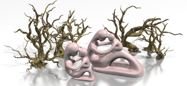
Figure 1: Variational subspace provides robust and high quality deformation results regarding arbitrary constraints at runtime. This figure shows tree and fertility as well as their deformed versions.

2 Mathematical Background

Consider minimizing a quadratic function $f(X;q)=(1/2)X^{T}HX-q^{T}X$ subject to linear constraints $A^{T}X=b$, where $X\in\mathbb{R}^{n}$ is an overly high dimensional solution, $H$ is a semi-definite positive matrix of size $n\times n$, $q\in\mathbb{R}^{n}$, $A$ is a well-conditioned matrix of size $n\times m$, and $b\in\mathbb{R}^{m}$. Typically, $m\ll n$. Without loss of generality, we can write

$$\begin{array}[]{rl}\min_{X}&(1/2)X^{T}HX-q^{T}X\\ \text{s.t.}&A^{T}X=b.\end{array}$$ (1)

Instead of solving the optimization with a single setup, we consider a set of them with a prescribed fixed $H$, and varying $A$, $b$ and $q$ under certain conditions. The “demand” of this configuration is defined to be a particular choice of $A$, $b$ and $q$. Different choices usually result in different optimum solutions. When $n$ is relatively small, efficiently solving for unreduced solutions belongs to the family, so called multi-parametric quadratic programming, or mp-QP [Bemporad et al. 2002][Tøndel et al. 2003]. We instead approach to tackle the same setting with a large $n$ by exploring approximate solutions in a carefully chosen low-order space.

We model the “demand”s by assuming each column of $A_{n\times m}$ is selected from a low-order linear space $C_{n\times d}$, namely $A=C_{n\times d}A_{c}\in\operatorname{Span}(C)$ for some $A_{c}$, and $q$ is again selected from another low-order linear space $\operatorname{Span}(D)$ such that that $q=D_{n\times k}Y$ for some $Y$, where $A_{c}$ is a matrix of size $d\times m$, $Y$ is a vector of size $k\times 1$. Here $d$ and $k$ is the dimension of reduced subspace $C$ and $D$ articulating to what $A$ and $q$ belong, respectively. Instead of pursuing a direct reduction in domain of solution $X$, we analyze the reducibility of “demand” parameters $A$ and $q$ by constructing reduced space $C$ and $D$. Specifications of the on-site parameters $A_{c}$, $b$ and $Y$ turn out to be the realization of “demand”s. We can rewrite (1) as

$$\begin{array}[]{rl}\min_{X,Z}&(1/2)X^{T}HX-Y^{T}D_{n\times k}^{T}X\\ \text{s.t.}&C_{n\times d}^{T}X=Z,\hskip 10.00002ptA_{c}^{T}Z=b.\end{array}$$ (2)

Optimization (2) can be decomposed into an equivalent two-stage formulation, i.e.,

$$\min_{A_{c}^{T}Z=b}\{\min_{C^{T}X=Z}f(X;DY)\}.$$ (3)

Karush-Kuhn-Tucker (KKT) condition yields that the optimum point $X^{\ast}(Z,Y;C,D)$ for $\min_{C^{T}X=Z}f(X;DY)$ should satisfy linear equations

$$\left(\begin{array}[]{cc}H&C\\ C^{T}&0\end{array}\right)\left(\begin{array}[]{c}X^{\ast}\\ \Lambda\end{array}\right)=\left(\begin{array}[]{c}DY\\ Z\end{array}\right).$$ (4)

where $\Lambda$ is a Lagrange multiplier. Therefore $X^{\ast}(Z,Y;C,D)$ is affine in terms of on-site parameters $Z$ and $Y$, i.e.,

$$X^{\ast}(Z,Y;C,D)=N(;C)Z+U(;C)DY\hskip 2.70004pt,$$ (5)

where $N(;C)$ and $U(;C)D$ can be computed before $A_{c}$, $b$ and $Y$ are observed in solving the second stage of (3): From Eq. (4), each column of $N(;C)$ is computed through a preconditioned linear direct solver by setting $Z$ as the corresponding column of $I_{d\times d}$ with $Y=0$; And similarly, each column of $U(;C)D$ is linearly solved by setting $DY$ to be the corresponding column of $D_{n\times k}$ with $Z=0$. Remark it is particularly required that $C$ and $D$ has to be full-rank and well-conditioned (as will be specified later).

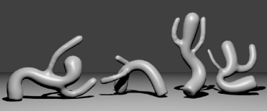
Figure 2: Artistic freedom is important in deformable mesh modeling because many artists are interested in authoring creative editing. Rig or cage based deformation lacks the richness of deformable variants.

Once we have a subspace design (5), for arbitrary “demand” $A$, $b$ and $q$, we can immediately solve for an approximate solution $X^{*}(Z_{\min},Y_{\min})$ via substituting (5) into the original formulation (1). We clarify that if our assumption is held, i.e., $A=CA_{c}$ and $q=DY$ for some $A_{c}$ and $Y$, the approximate solution is identical to the exact optimal $X_{\min}$. Furthermore, the approximated solution can work with hard constraints in the online solvers.

In next, we demonstrate its effectiveness by implementing an interactive mesh deformation method based on the model reduction framework we proposed. In the end, we will return to the theoretical aspects, and derive an error bound for the approximate solution with respect to the use of $C$ and $D$.

3 Interactive Mesh Deformation

In this section, we start from the point that is familiar to the graphics audiences, and proceed to the practice of our reduced model, where we mainly focus on deriving the correct formulation for employing variational subspace. Experimental results are provided in the end. In order for practitioners to reproduce our framework, we describe the details of our implementation in Appendix B. We remark that, subspace techniques described in this section has been standardized as described in [Jacobson et al. 2012]. The main difference is to replace the original linear subspace of a skinning mesh with the variational subspace described in our paper. Our variational subspace techniques extends the fast deformable framework as proposed in [Jacobson et al. 2012] to meshes whose skinning is not available or impossible, such as those of complex typologies. There are, however, good reasons to work with linear blending skinning, for example, it is often possible for artists to directly edit the weights painted on a skinned mesh.

Notations. Denote by $\mathbf{v}_{1},\ldots,\mathbf{v}_{n}\in\mathbb{R}^{3}$ the rest-pose vertex positions of input mesh $\mathcal{M}$, and denote the deformed vertex positions by $\mathbf{v}^{\prime}_{1},\ldots,\mathbf{v}^{\prime}_{n}\in\mathbb{R}^{3}$.

Use bold lowercase letters to denote single vertex $\mathbf{v}\in\mathbb{R}^{3}$ and $3\times 3$ transformation matrix $\mathbf{r}$, and bold uppercase letters $\mathbf{V}$ and $\mathbf{R}$ to denote arrays of them. We use uppercase normal font letters to denote general matrices and vectors (one column matrices) and lowercase normal letters to denote scalars. We may or may not specify the dimensions of matrices explicitly in the subscripts, hence $M_{n\times n}$ and $M$ are the same. For some other cases, subscripts are enumerators or instance indicators. We use superscripts with braces for enumerators for matrices, e.g., $M^{(i)}$.

Use $\left\|\cdot\right\|$ to denote Frobenius norm of matrices (vectors), $\left\|\cdot\right\|_{2}$ to denote $L_{2}$ norm of matrices, and $\left\|Z\right\|_{M}=\sqrt{\mbox{tr}(Z^{T}MZ)}$ to denote Mahalanobis norm with semi-positive definite matrix $M$.

Denote dot product of matrices by $\circ$, and Kronecker product of matrices by $\otimes$. Let $I$ be the identity matrix, $\mathbf{0}$ be the zero matrix and $\mathbf{1}$ be a matrix of all ones.

3.1 Variational Reduced Deformable Model

ARAP energy. In recent development of nonlinear deformation energy, the As-Rigid-As-Possible energy [Sorkine and Alexa 2007, Xu et al. 2007, Chao et al. 2010] is welcomed in many related works, in which they represent deformations by local frame transformation. The objective energy function under this representation is quadratic in terms of variables: vertices and transformation matrices with orthogonality constraints. This family of energy functions can be written as

$$\mathcal{E}(\mathbf{V}^{\prime},\mathbf{R})=\frac{1}{2}\sum\limits_{k=1}^{r}\sum\limits_{(i,j)\in\mathcal{G}_{k}}\!\!\!c_{ijk}\left\|(\mathbf{v}^{\prime}_{i}\!-\!\mathbf{v}^{\prime}_{j})\!-\!\mathbf{r}_{k}(\mathbf{v}_{i}\!-\!\mathbf{v}_{j})\right\|^{2}\;,$$ (6)

where $\mathcal{G}_{k}$ are their corresponding sets of edges (see Figure 5 of [Jacobson et al. 2012]), $c_{ijk}\in\mathbb{R}$ are typically the cotangent weights [Chao et al. 2010], and $\mathbf{r}_{k}\in SO(3)$ denotes the local frame rotations. By separating quadratic terms and linear terms w.r.t. $\mathbf{v}_{i}$, and vectorizing $(\mathbf{v}_{i})_{i=1}^{n}$ and $(\mathbf{r}_{k})_{k=1}^{r}$ to $V^{\prime}_{3n\times 1}$ and $R_{9r\times 1}$ respectively, ARAP energy can be further expressed as

$$E(V^{\prime},R)=\frac{1}{2}V^{\prime T}HV^{\prime}-R^{T}KV^{\prime}+\mbox{constant},$$ (7)

where $\mathbf{r}_{k}^{T}\mathbf{r}_{k}=I_{3\times 3}$ (see [Jacobson et al. 2012] for more details).

Rotational proxies. By observation, minimizing ARAP energy involves solving $R$, which is in complexity of mesh geometries. We modify the original ARAP energy to a piece-wise linear form, which relieves the high non-linearity of optimization, but simultaneously increases the complexity by introducing linearization variables.

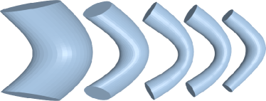
Figure 3: Results subject to different regularization coefficients. Deformed solid cylinder upon three point constraints. From left to right: $\alpha=0.01,0.05,0.1,1,10$.

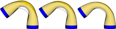
Figure 4: Results with varied number of rotational proxies. From Left to right: $d=5,9,17$: for each, deformed result with 32 rotational proxies is shown with dark contours.

We divide $r$ local rotations into $d$ rotational clusters spatially, which is an over-segmentation of input meshes. Rotations within each patch segment are desired to be similar in deformations. Empirically, we found that a simple k-means clustering on weighted Laplacian-Beltrami eigen-vectors fits well with our scheme, which cuts surface/solid mesh into $d$ patches. We revise the original energy by assuming

$$\mathbf{r}_{k}\approx\mathbf{s}_{i_{k}}+\mathbf{q}_{k}\;,$$ (8)

where $\mathbf{s}_{i_{k}}\in SO(3)$ denotes $i_{k}$-th patch-wise frame rotation of the cluster that the vertex $k$ belongs, and

$$\mathbf{q}_{k}=\begin{pmatrix}q_{0}&-q_{3}&q_{2}\\ q_{3}&q_{0}&-q_{1}\\ -q_{2}&q_{1}&q_{0}\end{pmatrix}^{(k)}=\sum_{i=0}^{3}q^{(k)}_{i}\mathbf{d}_{i}\;.$$ (9)

It should be noted that Laplacian surface editing [Sorkine et al. 2004] utilizes $\mathbf{q}_{k}$ to approximate the rotation matrix, whereas we use $\mathbf{q}_{k}$ to approximate the difference of two rotation matrices $\mathbf{r}_{k}-\mathbf{s}_{i_{k}}$. It leads to a different energy by appending L2 penalties subject to the regulators $\mathbf{q}_{k}$:

$$\mathcal{E}^{\prime}(\mathbf{V}^{\prime},\mathbf{Q},\mathbf{S})=\mathcal{E}(\mathbf{V}^{\prime},\mathbf{S}+\mathbf{Q})+\alpha\sum_{k=1}^{r}a_{k}\left\|\mathbf{q}_{k}\right\|^{2}+\beta\sum_{k=1}^{r}a_{k}\left\|\mathbf{q}_{k}\mathbf{n}_{k}\right\|^{2},$$ (10)

where $a_{k}$ denotes the element-wise area/volume, $\alpha$ denotes the penalty coefficient of overall spatial distortion, and $\beta$ denotes the additional penalty coefficient of surface normal distortion (if applicable). $\alpha$ and $\beta$ are empirically chosen. (See Fig. 3 for deformations subject to different penalty coefficients $\alpha+\beta$). One potential issue is that using this penalty may incur surface folds when shapes are bended at large angles. To counteract such effects, we optionally use an extra regularization term appended to $\mathcal{E}^{\prime}(\mathbf{V}^{\prime},\mathbf{Q},\mathbf{S})$ penalizing the moving frame differentials [Lipman et al. 2007], i.e.,

$$\gamma\sum_{(k,j)\in\mathcal{H}}a_{k,j}\left\|\mathbf{s}_{i_{k}}\!\!+\!\mathbf{q}_{k}\!\!-\!\mathbf{s}_{i_{j}}\!\!-\!\mathbf{q}_{j}\right\|^{2},$$ (11)

where $\mathcal{H}$ is the set of neighboring local frames and $a_{k,j}=(a_{k}+a_{j})/2$. The two bending cylinder examples in Fig. 8 are produced by penalizing the moving frame differentials.

Let $S_{9d\times 1}$ and $Q_{4r\times 1}$ be the vectorization of $(\mathbf{s}_{i})$ and $(\mathbf{q}_{k})$ respectively. $\mathcal{E}^{\prime}$ is quadratic in terms of $\mathbf{V}^{\prime}$ and $\mathbf{Q}$, and its partial gradient w.r.t. $\mathbf{V}^{\prime}$ and $\mathbf{Q}$ is again linear in terms of $\mathbf{S}$. Hence again we can write $\mathcal{E}^{\prime}$ as

$$E^{\prime}(V^{\prime},Q,S)=\frac{1}{2}[V;Q]^{T}L[V;Q]-S^{T}M[V;Q]+S^{T}NS+\mbox{constant}\;,$$

where $S$ are the rotational proxies of our model, $N\neq\mathbf{0}$ iff the extra regularization (11) is present.

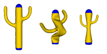
Figure 9: Left: Original model; Middle: Out-of-shape distortion in ARAP surface modeling; Right: Our method deforms rest-pose part via shrinking.

There is an interesting discussion about the difference between $\mathcal{E}$ and $\mathcal{E}^{\prime}$, because $\mathcal{E}^{\prime}$ includes near-isotropic scaling which has arguable values over distortion in only one direction for artistic modeling purpose in case the desired deformation is far from the isometry [Sorkine et al. 2004, Lipman et al. 2008]. (See Fig. 9 for comparison with the ARAP energy.)

Linear proxies. Besides rotational proxies, we add $3m$ linear proxies via pseudo-spatial linear constraints,

$$W_{3m\times 3n}V^{\prime}=X\;,$$ (12)

where $X$ are the linear proxies of our model.

Intuitively, $W=\widehat{W}_{m\times n}\otimes I_{3\times 3}$ spans a finite dimensional linear space to approach the uncertainty set of onsite constraints provided by users. Its choice reflects how we reduce the dimension of anticipated constraints, as suggested by the use of variational subspace, A simple choice is a sparse sampling of $m$ vertices (shown as Fig. 5), i.e (under a permutation)

$$W_{3n\times 3m}=\{\ldots;\overbrace{0,\ldots,0,1,0,\ldots,0}^{\mbox{\small sample at singe vertex i}};\ldots\}_{n\times m}\otimes I_{3\times 3},$$

and an alternative one is to utilize $m$ vertices groups via clustering, i.e., (under a permutation)

$$W_{3n\times 3m}=\dfrac{1}{\mathcal{N}}\{\ldots;\underbrace{\ldots,0,\!\!\!\!\!\!\!\!\!\!\!\!\!\overbrace{1,\ldots,1}^{\mbox{\small vertices group j of size $\mathcal{N}$}}\!\!\!\!\!\!\!\!\!\!\!\!\!,0,\ldots}_{\mbox{\small j-th rows}};\ldots\}_{n\times m}\otimes I_{3\times 3}.$$

To this point, technically contrast with our approach, standard model reduction technique employ a strategy that vertices are explicitly represented in low-order by $V^{\prime}_{3n\times 1}=K_{3n\times 3m}X_{3m\times 1}$. In order to compute a reasonable subspace, different smoothness criterion are exposed on computing $K$, such as heat equilibrium[Baran and Popović 2007], exponential propagating weights[Jacobson et al. 2012], biharmonic smoothness[Jacobson et al. 2011]. We instead reduce the dimension of constraints, and the subspace are then automatically solved accordingly.

Variational subspace. With context of approximated energy $E^{\prime}$, we are to solve the linear variational problem so as to derive a reduced representation of $V^{\prime}$ in terms of proxies $S$ and $X$, i.e.,

$$\begin{array}[]{rl}\min\limits_{V^{\prime},Q}&E^{\prime}(V^{\prime},Q,S)\\ \mbox{s.t.}&W_{3m\times 3n}V^{\prime}=X\;.\end{array}$$ (13)

By KKT condition introducing Lagrange multipliers $\Lambda$, we have a set of linear equations in respect of $V^{\prime},Q,\Lambda$, which can be expressed as matrix form

$$\begin{pmatrix}L&W^{T}\\ W&0\end{pmatrix}[V^{\prime};Q;\Lambda]=[M^{T}S;X]\;.$$ (14)

This then implicitly establishes a linear map

$$\begin{array}[]{rcl}[V^{\prime};Q]&=&N_{W}X+U_{W}S\;,\end{array}$$ (15)

where each column of matrices $N_{W},U_{W}$ can be pre-computed by a sparse linear solver with a single preconditioning (LU or Cholesky), subject to each single variable in vector $X$ and $S$. Solving for $N_{W}$ and $U_{W}$ only need one time computation in the offline stage.

Sub-manifold integration. Provided variational subspace, $X$ and $S$ span a sub-manifold of deformations. We then restrict our scope to determine reduced variables $X$ and $S$. We employ a routine similar to alternating least square [Sorkine and Alexa 2007], where we alternatively update $X$ and $S$ via two phases.

Phase 1: provided $S^{(i)}$, solve for $X^{(i)}$.

By substituting (15) into approximated ARAP energy (3.1), we derive a reduced ARAP energy as

$$E^{\prime\prime}(S,X)=\frac{1}{2}X^{T}\widetilde{L}X-S^{T}\widetilde{M}X+\mbox{constant}\;.$$ (16)

where $\widetilde{L}=(N_{W})^{T}LN_{W}$ and $\widetilde{M}=MN_{W}+(U_{W})^{T}LN_{W}$. With onset hard constraints $W_{\mbox{\scriptsize eq}}V^{\prime}=P_{\mbox{\scriptsize eq}}$ specified by the user (where $W_{\mbox{\scriptsize eq}}$ are positional constraints and $P_{\mbox{\scriptsize eq}}$ are their values), we are then to solve for linear proxies $X$

$$\begin{array}[]{rl}\min\limits_{X}&E^{\prime\prime}(S^{(i)},X)\\ \mbox{s.t.}&N_{\mbox{\scriptsize eq}}X=P_{\mbox{\scriptsize eq}}-U_{\mathrm{eq}}S^{(i)}\end{array}$$ (17)

where $N_{\mbox{\scriptsize eq}}=W_{\mbox{\scriptsize eq}}N_{W},U_{\mbox{\scriptsize eq}}=W_{\mbox{\scriptsize eq}}U_{W}$. Hard constraints are the default setting of our framework.

Alternatively, we can pose on-site soft constraints as

$$\begin{array}[]{rl}\min\limits_{X}&E^{\prime\prime}(S^{(i)},X)+\delta\left\|N_{\mbox{\scriptsize eq}}X+U_{\mathrm{eq}}S^{(i)}-P_{\mbox{\scriptsize eq}}\right\|^{2},\end{array}$$ (18)

where $\delta\!\!>\!\!0$ is adjusted interactively by user to match the desired effects. We input $W_{\mbox{\scriptsize eq}},P_{\mbox{\scriptsize eq}}$ and solve the integrated reduced model interactively.

Remark that because optimization problems (equations (17) and (18)) are again linear variational, it can be efficiently solved by a standard dense linear solver: (1) pre-computing LU factorization of matrix (not related to $S$) at the stage to specify constraint handlers $W_{\mbox{\scriptsize eq}}$, and (2) backward substitution on the fly at the stage to drag/rotate handler.

Phase 2: provided $X^{(i)}$ and $S^{(i)}$, compute $S^{(i+1)}$. Rather than minimizing the reduced energy functional $E^{\prime\prime}$ (shown in Eq. (16)) in terms of $S$, we instead want rotational clusters to adapt for the existing deformation. Letting $[V^{\prime(i)};Q^{(i)}]=N_{W}X^{(i)}+U_{W}S^{(i)}$, we fit a patch-wise local frame of rotational clusters subject to deformed mesh $V^{\prime(i)}$ by dumping relations $Q^{(i)}$ and their penalties $\alpha\!\!=\!\!\beta\!\!=\!\!\gamma\!\!=\!\!0$, and optimizing a simplified energy $\mathcal{E}(\mathbf{V}^{\prime(i)},\mathbf{S})=E^{\prime}(V^{\prime(i)},\mathbf{0},S)$, which is equivalent to

$$\begin{array}[]{rl}\max\limits_{S}&S^{T}M[V^{\prime(i)};\mathbf{0}]=S^{T}(M_{N}X^{(i)}+M_{U}S^{(i)})\\ \mbox{s.t.}&\mathbf{s}_{i}\in SO(3),\quad i=1,\ldots,d,\end{array}$$ (19)

where $M_{N}$ and $M_{U}$ are pre-computed. It is well known that those rotation fittings can be solved in parallel via singular value decomposition of each gradient block of $\mathbf{s}_{i}$. For $3\times 3$ matrix, we employ the optimized SVD routines by McAdams and colleagues [McAdams et al. 2011] that avoid reflection, i.e., guarantee the orientation.

3.2 Algorithm overview

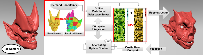
Figure 5: Interactive mesh modeling framework of our approach. From left to right: (1) Input red demon model $V$; (2) Pre-process to set pseudo-constraint points as linear proxies and near-rigid parts as rotational proxies; (3) Compute variational subspace $N_{W},U_{W}$ offline, and load into display device. (4) Prepare subspace integration $\widetilde{L}$, $\widetilde{M}$, $M_{N}$ and $M_{U}$. (5) At run-time, given on-site user demand $W_{\mbox{\scriptsize eq}},P_{\mbox{\scriptsize eq}}$, solve for reduced variables $X,S$ and upload to display device (bandwidth saving); (6) Display deformed mesh and feedback.

We review our previous mathematical formulations, and summarize our algorithm into three stages (see also Fig. 5):

Pre-compute. The user loads initial mesh model $\mathcal{M}$, linear proxies $W$, rotational proxies $(i_{k})$, and affine controllers (if applicable). Our algorithm constructs a sparse linear system to solve for variational subspace $N_{W}$ and $U_{W}$, and then pre-computes $\widetilde{L}$, $\widetilde{M}$, $M_{N}$ and $M_{U}$.

Prepare on-site constraints. When above pre-computed matrices are present, the user can only freely specify the intended constraint handler on-site. They are in the form of $W_{\mbox{\scriptsize eq}}$. Our algorithm then proceeds to compute $N_{\mbox{\scriptsize eq}}$ and $U_{\mbox{\scriptsize eq}}$, and pre-factorize the linear system (see equation (17) or (18)). If a user introduces a brand new set of constraints on-site, this stage will be re-computed within tens of milliseconds. The timing regard to different settings has been reported in Table 1 column “OP”.

Deform on the fly. Our algorithm allows the user to deform meshes on the fly, which means the user can view the deformation results instantly by controlling constraint handlers. For each frame, our model takes in positional constraints $P_{\mbox{\scriptsize eq}}$, calls an alternating routine (with global rotation adaption) interactively to solve for proxy variables $X$ and $S$, and reconstructs and displays the deformed mesh. To guarantee real-time performance, we used a fixed number of iterations per frame. By initializing an alternating routine with the previous frame proxies, we do not observe any disturbing artifacts even when using only 8 iterations.

3.3 Results and Discussion

	Input Model		Proxies		Runtime			Pre-computation
Model	Vert.	Type	Linear	Rot.	1 Iter. ($\mu$s)	Df. (ms)	Total (ms)	Subspace (s/GB)	OP (ms)	Fig.
Cylinder	5k	Tri.	33	12	50	1.4	2	14 (0.3)	14	8
Cactus	5k	Tri.	33	27	90	2	3	18 (0.4)	16	8
Bar	6k	Tri.	33	52	93	3.8	4.8	36 (.5)	20	8
Bumpy Plane	40k	Tri.	33	27	85	14	15	200 (2.7)	38	8
Plate Box	4k	Tet.	25	25	62	2	2.7	30(.4)	11	6
Solid Cylinder	8k	Tet.	33	52	110	4	5	90 (.8)	22	3
Tree	3.6k	Tri.	60	60	137	3.5	5	34(.4)	10	1
Fertility	25k	Tet.	29	26	78	5.2	6	148 (2.4)	28	1
Dinosaur	21k	Tri.	46	34	108	12	14	115 (1.7)	24	7
Dragon	53k	Tri.	20	20	55	14	15	198 (2.7)	64	10
Red Demon	80k	Tri.	30	28	90	35	36	498 (5.8)	106	5

Table 1: Model statistics and serial performance on a HP laptop with an Intel i7 2.20GHz _×8 Processor. From left to right: number of vertices, type of mesh, number of linear proxies, number of rotational proxies, time in $\mu$ seconds for one iteration, time in milliseconds for mapping reduced solution info full space (Intel MKL on CPU performance), time in milliseconds for full optimization per frame, time in seconds (and memory in GBytes) for pre-computation of subspace, time in milliseconds for computation of on-site preconditioner, figure that shows the configuration.

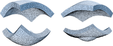
Figure 6: Our reduced model preserves the nature of different functions. Left: volumetric deformed mesh; Right: deformed surface (self-occlusion possible) under same constraints.

Figure 7: Our revised energy does not reveal linearization artifacts when the deformation is isometric (middle). It also favors isotropic scaling when the model is stretched or shrunk (right). The original model is shown in the left.

We implement our framework for deformable mesh modeling and demonstrate our results by examples which include standard deformation suites introduced in [Botsch and Sorkine 2008]. Results of our approach on a set of typical test meshes are shown in Fig. 8). The results shown can be compared with results of high quality methods without model reduction, including PriMo[Botsch et al. 2006], also shown in [Botsch and Sorkine 2008]. Besides, we also demonstrate the strength of our method in conformal setting, where we configure scaling factors in our modeling framework (see Fig. 10). In our experiments, the modeling framework runs robustly on various models, for different types of transformation, such as small and large rotations, twisting, bending, and more as shown in Fig. 2. It works reasonably naturally on both surface and solid meshes, in which user’s choice of energy controls the desired behaviors (see Fig. 6). It also accommodates different hyper-parameter setting, such as the number and type of proxies, to produce predictable and reasonable results (see Fig. 4).

Based on our CPU implementation, We report timing of our algorithm working on different models presented in our paper in Table 1. All timing results are generated on an Intel Core${}^{\mbox{\scriptsize TM}}$ i7-2670QM 2.2GHz $\times$8 processor with 12 GB RAM. It has been shown that the time used in reduced model iteration is not related to the geometric complexity, and the overall computation per frame is magnitude faster than that as reported in [Hildebrandt et al. 2011]. The computational framework used in our paper is almost as same as the one used in [Jacobson et al. 2012], thus the performances are comparable. It is also shown that the process of mesh reconstruction, which is a matrix-vector product (see Eq. (15) and column “Df.” of Table 1), is the bottle-neck of overall computation, yet it is embarrassingly parallel.

Figure 8: Approximation quality of our method in all images is demonstrated on the test suite of models introduced in [Botsch and Sorkine 2008]; From left to right: Bumpy Plane, Cylinder, Cactus, Bar. Multiple types of deformations, including bending, shifting and twisting, are tested.

Comparing to other cell-based model reduction methods [Sumner et al. 2007, Botsch et al. 2007], our approach utilizes a much smaller number of reduced variables. Typically, we adopt no more than 35 linear proxies, and no more than 60 rotational proxies. Besides, the configuration of proxies gives user the freedom to design his/her own needs in modeling a particular mesh. Instead restricting variability in modes and modal derivatives space [Hildebrandt et al. 2011], artist, based on his intentions, can cut shape into near rigid parts (each for a rotational proxy), and specify pseudo constrain locations as linear proxies. Fig. 5 demonstrates a modeling scenario where artist intended to adjust mouth, nose and eyes on a face model: semantic parts are in first annotated, variational reduced deformable model is then pre-computed for on-line editing.

4 Theory of Variational Subspace

The notations used follows the preliminary setup in section 2.

4.1 Concept of Approximation

Definition 4.1 (Variational Subspace).

Given a quadratic programming problem in the form of Eq. (1), choose $C$ and $D$ for the problem in the two-stage form as Eq. (3). The solution $X^{\ast}(Z,Y;C,D)$ for the first stage problem is hence given by Eq. (5). The subspace spanned by columns of $N$ and $U\cdot D$ are called variational subspace.

Proposition 4.1.

$N$ is a matrix of size $n\times d$ and $U\cdot D$ is a matrix of size $n\times k$. Their columns span a linear subspace $\operatorname{Span}(U)+\operatorname{Span}(U\cdot D)$ where the reduced solution belongs. Those columns are computed by solving a variational formulation provided by Eq. (4).

In Eq. 1, $H$ is only guaranteed to be positive semi-definite. We have Cholesky decomposition $H=L^{T}L$, where $L$ is upper triangular with non-negative diagonal entries [Golub and Van Loan 2012]. Denote the pseudo-inverse of $L$ by $L^{+}$, then for any $X\in\mathbb{R}^{n}$, we have a two-part orthogonal decomposition $X=\tilde{X}+\bar{X}$, where

$$\tilde{X}=L^{+}LX,\hskip 10.00002pt\bar{X}=(I-L^{+}L)X.$$ (20)

Proposition 4.2.

With the two-part decomposition Eq. (20), we have

$$L\tilde{X}=LX,\hskip 10.00002ptL\bar{X}=0,\hskip 10.00002pt\tilde{X}^{T}\bar{X}=0.$$ (21)

In addition, if $H=L^{T}L$ is positive definite, $\bar{X}=0$.

Moreover, we can rewrite the optimization problem Eq. (1) as

$$\begin{array}[]{rl}\min_{X}&(1/2)(\tilde{X}+\bar{X})^{T}L^{T}L(\tilde{X}+\bar{X})-q^{T}(\tilde{X}+\bar{X})\\ \text{s.t.}&A^{T}(\tilde{X}+\bar{X})=b\\ &\tilde{X}=L^{+}LX,\hskip 10.00002pt\bar{X}=(I-L^{+}L)X.\end{array}$$ (22)

Since $L\bar{X}=0$, we simplify above formulation to

$$\begin{array}[]{rl}\min_{X}&f(X)=(1/2)\tilde{X}^{T}L^{T}L\tilde{X}-q^{T}\tilde{X}-q^{T}\bar{X}\\ \text{s.t.}&A^{T}\tilde{X}=b-A^{T}\bar{X}\\ &\tilde{X}=L^{+}LX,\hskip 10.00002pt\bar{X}=(I-L^{+}L)X.\end{array}$$ (23)

It is observed that only $\tilde{X}$ appears in second-order term in the objective function of Eq (23). Suppose the optimal solution to Eq. (1) is $X_{\min}$ with a two-part decomposition (given by Eq. (20)) $X_{\min}=\tilde{X}_{\min}+\bar{X}_{\min}$, we then consider the following companion optimization problem

$$\begin{array}[]{rl}\min_{\tilde{X}}&\tilde{f}(\hat{X})=(1/2)\tilde{X}^{T}L^{T}L\tilde{X}-q^{T}\tilde{X}-q^{T}\bar{X}_{\min}\\ \text{s.t.}&A^{T}\tilde{X}=b-A^{T}\bar{X}_{\min}\\ &(I-L^{+}L)\tilde{X}=0.\end{array}$$ (24)

Remark $-q^{T}\bar{X}_{\min}$ which appears in objective function of Eq. (24) is a constant. We see Eq. (24) can be equivalently solved in two steps: In the first step, we solve the following problem

$$\begin{array}[]{rl}\min_{\tilde{X}}&\tilde{f}(\tilde{X})+q^{T}\bar{X}_{\min}=(1/2)\tilde{X}^{T}L^{T}L\tilde{X}-q^{T}\tilde{X}\\ \text{s.t.}&A^{T}\tilde{X}=b-A^{T}\bar{X}_{\min}.\end{array}$$ (25)

And in the second stage, we project the solution to $L^{+}L\tilde{X}_{\min}$, where $\tilde{X}_{\min}$ is the solution to Eq. (25).

Theorem 4.3.

Suppose $X_{\min}$ is the unique solution to Eq. (23), $\tilde{X}^{\circ}_{\min}$ is the unique solution to Eq. (24), and $\tilde{X}_{\min}$ is the unique solution to Eq. (25), then we have $\tilde{X}_{\min}^{\circ}=L^{+}LX_{\min}=L^{+}L\tilde{X}_{\min}$.

Proof.

We observe that $L^{+}LX_{\min}$ satisfies the constraint of Eq. (24), and objective functions of Eq. (23) and Eq. (24) coincide, i.e., $f(X_{\min})=\tilde{f}(L^{+}LX_{\min})$. Therefore, as $\tilde{X}^{\circ}_{\min}$ is the minimizer to Eq. (24), we have

$$f(X_{\min})\geq\tilde{f}(\tilde{X}^{\circ}_{\min}).$$

On the other hand, $\tilde{f}(\tilde{X}^{\circ}_{\min})=f(\tilde{X}^{\circ}_{\min}+\bar{X}_{\min})$. Given $X_{\min}$ is the minimizer to Eq. (23), we also have

$$\tilde{f}(\tilde{X}^{\circ}_{\min})\geq f(X_{\min}).$$

Hence, the equality holds for $\tilde{f}(\tilde{X}^{\circ}_{\min})=f(X_{\min})$. Given that the optimum exists and is unique, we have

$$\tilde{X}^{\circ}_{\min}+\bar{X}_{\min}=X_{\min}\Rightarrow\tilde{X}^{\circ}_{\min}=L^{+}LX_{\min}.$$

The proof of $\tilde{X}_{\min}^{\circ}=L^{+}L\tilde{X}_{\min}$ is similar: observe that $\tilde{f}(\tilde{X}^{\circ}_{\min})=\tilde{f}(L^{+}L\tilde{X}_{\min})$ and $L^{+}L\tilde{X}_{\min}$ satisfies the constraint of Eq. (24). ∎

Definition 4.2.

Two solutions subject to the form Eq. (1) (parameterized by $A$, $q$, and $b$) are called quotient equivalent, if they share the same companion problem defined by Eq. (25), i.e. their $\hat{b}(A,b,q)=b-A^{T}\bar{X}_{\min}$ are the same. This forms group equivalence in the space of solutions.

For example, let $H$ be the Laplacian operator $\Delta$, the solution would minimize the the L2 norm of first-order gradient. In such case, two problems are of quotient equivalence if their optimal solutions preserve to an additive constant. We use the distance between two solution groups under the quotient equivalence to measure the approximation error. It is the Mahalanobis distance provided by $H$, i.e.

$$d_{H}(x,y)=(x-y)^{T}H(x-y)=(Lx-Ly)^{T}(Lx-Ly).$$

Let $LX=\hat{X}$, $\hat{q}=L^{+}q$, $\hat{A}=L^{+}A$, and $\hat{b}=b-A^{T}\bar{X}_{\min}$, we rewrite Eq. (25) (but not equivalent) as

$$\begin{array}[]{rl}\min_{\hat{X}}&(1/2)\hat{X}^{T}\hat{X}-\hat{q}^{T}\hat{X}\\ \text{s.t.}&\hat{A}^{T}\hat{X}=\hat{b}\\ &(I-LL^{+})\hat{X}=0.\end{array}$$ (26)

Similar to the treatment of Eq. (24), we can in first solve

$$\begin{array}[]{rl}\min_{\hat{X}}&(1/2)\hat{X}^{T}\hat{X}-\hat{q}^{T}\hat{X}\\ \text{s.t.}&\hat{A}^{T}\hat{X}=\hat{b}.\end{array}$$ (27)

and then project the solution to $LL^{+}\hat{X}_{\min}$, where $\hat{X}_{\min}$ is the solution to Eq. (27).

Since we are always interested in distance measure $d_{H}$ for different solutions, the projection step in solving Eq. (24) is not necessary to compute $d_{H}$. The distance between two solution groups $X_{1}$ and $X_{2}$ of the quotient equivalence is therefore the Euclidean distance between $\hat{X}_{1}=LX_{1}$ and $\hat{X}_{2}=LX_{2}$.

Similar to the treatment of Eq. (1) and Eq. (27), we can derive the two-stage problem from Eq. (2) as

$$\begin{array}[]{rl}\min_{\hat{X}}&(1/2)\hat{X}^{T}\hat{X}-\hat{Y}^{T}\hat{D}^{T}\hat{X}\\ \text{s.t.}&\hat{C}^{T}\hat{X}=\hat{Z}\\ &A_{C}^{T}\hat{Z}=\hat{b},\end{array}$$ (28)

where $\hat{D}=(L^{+})^{T}D$ and $\hat{C}=(L^{+})^{T}C$. The KKT condition of its first-stage problem is given similarly as

$$\left(\begin{array}[]{cc}I&\hat{C}\\ \hat{C}^{T}&0\end{array}\right)\left(\begin{array}[]{c}\hat{X}^{\ast}\\ \Lambda\end{array}\right)=\left(\begin{array}[]{c}\hat{D}\hat{Y}\\ \hat{Z}\end{array}\right).$$ (29)

where $\Lambda$ is a Lagrange multiplier. We have the following justifications to only study Eq. (27) and Eq. (28).

Proposition 4.4.

If $X_{\min}$ is the optimal solution to Eq. (1) and $\hat{X}_{\min}$ the optimal solution to Eq. (27) with $\bar{X}_{\min}=(I-L^{+}L)X_{\min}$ and $\hat{b}=b-A^{T}\bar{X}_{\min}$, we have $LX_{\min}=LL^{+}\hat{X}_{\min}$. The similar argument also holds for Eq. (2) and Eq. (28).

Proof.

Because $L^{+}LX_{\min}$ is the optimal solution to Eq. (23), we have $L^{+}LX_{\min}=L^{+}L\tilde{X}_{\min}$, where $\tilde{X}_{\min}$, as mentioned, is the optimal solution to Eq. (25). On the other hand, we know $L\tilde{X}_{\min}=LL^{+}\hat{X}_{\min}$. Therefore, we have $L(L^{+}LX_{\min}-L^{+}\hat{X}_{\min})=0\Rightarrow LX_{\min}=LL^{+}\hat{X}_{\min}$. ∎

Proposition 4.5.

Suppose $X^{\ast}=NZ+UDY$ is the solution of Eq. (4) and $\hat{X}^{\ast}=\hat{N}\hat{Z}+\hat{U}\hat{D}\hat{Y}$ is the solution of Eq. (29), we have $LX^{\ast}=\hat{X}^{\ast}$ if $\hat{Z}=Z-C^{T}(I-L^{+}L)X^{\ast}$ and $\hat{Y}=Y$.

Proof.

We have $(L^{+})^{T}(L^{T}LX^{\ast}+C\Lambda-DY)=0\Rightarrow LX^{\ast}+\hat{C}\Lambda-\hat{D}Y=0$ and $C^{T}L^{+}LX^{\ast}=Z-C^{T}(I-L^{+}L)X^{\ast}\Rightarrow\hat{C}^{T}LX^{\ast}=\hat{Z}$. Therefore, $LX^{\ast}$ satisfies Eq. (29). ∎

Definition 4.3 (Variational Subspace Under Quotient Equivalence).

Given $\hat{X}^{\ast}=\hat{N}\hat{Z}+\hat{U}\hat{D}\hat{Y}$ to be the solution to Eq. (29), the columns of $\hat{N}$ and $\hat{U}\cdot\hat{D}$ span the variational subspace $\operatorname{Span}(\hat{N})+\operatorname{Span}(\hat{U}\cdot\hat{D})$ for solutions of optimization problem in the form of Eq. (27).

The main problem is thus revealed: how close are the exact solution of Eq. (27) and subspace solution restricted in a variational subspace defined by Def. 4.3, where the closeness is measured by the Mahalanobis distance $d_{H}$ provided by $H=L^{T}L$.

4.2 Bound of Approximation Error

In this section, we provide the proof that the approximation error of model reduction by variational subspace can be bounded in $d_{H}$.

Proposition 4.6 (Exact Solution).

Assuming Eq. (27) has a unique solution which has finite optimum, such that $\hat{A}$ is a full-rank matrix. the solution is

$$\hat{X}_{\min}=(I-\hat{A}\hat{A}^{+})\hat{q}+(\hat{A}^{+})^{T}\hat{b},$$ (30)

where $\hat{A}^{+}=(\hat{A}^{T}\hat{A})^{-1}\hat{A}^{T}$ is the pseudo-inverse of $\hat{A}$.

Proof.

The KKT condition of Eq. (27) indicates $\hat{X}_{\min}=\hat{q}-\hat{A}\Lambda_{\min}$ and $\hat{A}^{T}\hat{X}_{\min}=\hat{b}$. This leads to $\hat{A}^{T}(\hat{q}-\hat{A}\Lambda_{\min})=\hat{b}$. Since $\hat{A}$ is full-rank, $\widehat{A}^{T}\hat{A}$ is invertible. Hence we have

$$\Lambda_{\min}=(\hat{A}^{T}\hat{A})^{-1}(\hat{A}^{T}\hat{q}-\hat{b}).$$ (31)

Plug-in $\hat{X}_{\min}=\hat{q}-\hat{A}\Lambda_{\min}$ yields Eq. (30). ∎

Similarly, we also have

Proposition 4.7.

Suppose $\hat{X}^{\ast}(\hat{Z},\hat{Y})=\hat{N}\hat{Z}+\hat{U}\hat{D}\hat{Y}$ is the solution of Eq. (29), then

$$\hat{N}=(\hat{C}^{+})^{T},\hskip 10.00002pt\hat{U}\hat{D}=(I-\hat{C}\hat{C}^{+})\hat{D},$$ (32)

where $\hat{C}^{+}=(\hat{C}^{T}\hat{C})^{-1}\hat{C}^{T}$ is pseudo-inverse of $\hat{C}$, and $\hat{U}=I-\hat{C}\hat{C}^{+}$ is the orthogonal projector onto the kernel of $\hat{C}^{T}$ [Golub and Van Loan 2012].

Here we remark that in order for any subspace solution $\widehat{X}^{\ast}(\hat{Z},\hat{Y})$ to have a unique low-dimensional coordinate $(\hat{Z},\hat{Y})$. We should require $\hat{C}$ and $\hat{D}$ to be linearly independent. This equivalently means $\hat{U}\hat{D}$ is full rank.

Theorem 4.8 (Projection on Variational Subspace).

Assume columns of $\hat{C}$ and $\hat{D}$ are linearly independent. Given any $X\in\mathbb{R}^{n}$, its closest point (under Euclidean distance) in a variational subspace $\hat{X}^{\ast}(\hat{Z},\hat{Y})$ given by Eq. (32) is

$$\hat{Y}=(\hat{U}\hat{D})^{+}X,\hskip 10.00002pt\hat{Z}=\hat{C}^{T}X,$$ (33)

and the closest point is

$$\hat{X}^{\ast}=(\hat{U}\hat{D}(\hat{U}\hat{D})^{+}+\hat{C}\hat{C}^{+})X,$$ (34)

where $(\hat{U}\hat{D})^{+}=(\hat{D}^{T}\hat{U}\hat{D})^{-1}\hat{D}^{T}\hat{U}^{T}$ and $\hat{U}=I-\hat{C}\hat{C}^{+}$.

Proof.

If $\hat{U}\hat{D}v=0$ for some $v\in\mathbbm{R}^{k}$, we have $\hat{D}v+\hat{C}u=0$, where $u=C^{+}v$. Since $\hat{C}$ and $\hat{D}$ are linearly independent, we have $u=0$ and $v=0$. Therefore, $\hat{U}\hat{D}$ is full-rank. Furthermore,  $\hat{D}^{T}\hat{U}\hat{D}=\widehat{D}^{T}\widehat{U}^{T}\hat{U}\hat{D}$ is invertible. The closest point to $X$ is to minimize

$$\min_{\hat{Z},\hat{Y}}\|\hat{X}^{\ast}(\hat{Z},\hat{Y})-X\|^{2},$$

whose partial gradient against $\hat{Z}$ and $\hat{Y}$ should be zero, i.e.,

$$\hat{N}^{T}(\hat{N}\hat{Z}+\hat{U}\hat{D}\hat{Y}-X)=0$$

and

$$\hat{D}^{T}\hat{U}^{T}(\hat{N}\hat{Z}+\hat{U}\hat{D}\hat{Y}-X)=0.$$

Notice that $\hat{N}^{T}\hat{U}=0$, $\hat{N}^{T}\hat{N}=(\hat{C}^{T}\hat{C})^{-1}$, $\hat{U}^{T}\hat{U}=\hat{U}$. Above equalities can be simplified to

$$(\hat{C}^{T}\hat{C})^{-1}\hat{Z}=\hat{N}^{T}X,\hskip 10.00002pt\hat{D}^{T}\hat{U}\hat{D}\hat{Y}=\hat{D}^{T}\hat{U}^{T}X.$$

Above equalities can be solved as

$$\hat{Z}=(\hat{C}^{T}\hat{C})\hat{N}^{T}X=\hat{C}^{T}X,\hskip 10.00002pt\hat{Y}=(\hat{D}^{T}\hat{U}\hat{D})^{-1}\hat{D}^{T}\hat{U}^{T}X.\qed$$

Next, we are to derive the analytic subspace solution.

Proposition 4.9 (Variational Subspace Solution).

Let $\hat{I}=\hat{U}\hat{D}(\hat{U}\hat{D})^{+}+\hat{C}\hat{C}^{+}$ be orthogonal projector onto the subspace $\operatorname{Span}(\hat{C})+\operatorname{Span}(\hat{D})$([Yanai et al. 2011], page 45), where $\hat{U}=I-\hat{C}\hat{C}^{+}$ the orthogonal projector onto the kernel of $\hat{C}^{T}$. Assuming $\hat{A}$ is full-rank, columns of $\hat{C}$ and $\hat{D}$ are linearly independent, and $(\hat{A}^{T}\hat{I}\hat{A})^{-1}$exists, the variational subspace solution to Eq. (27) is

$$\hat{X}^{\ast}_{\min}=\left(\hat{I}-\hat{A}_{p}\hat{A}_{p}^{+}\right)\hat{q}+(\hat{A}_{p}^{+})^{T}\hat{b}$$ (35)

where $\hat{A}_{p}=\hat{I}\hat{A}$ and $\hat{A}_{p}^{+}=\left(\hat{A}^{T}_{p}\hat{A}_{p}\right)^{-1}\hat{A}_{p}^{T}$. Note $\hat{I}-\hat{A}_{p}\hat{A}_{p}^{+}$ is the projection matrix restricted in subspace $\operatorname{Span}(\hat{C})+\operatorname{Span}(\hat{D})$ that map onto the kernel of $\hat{A}_{p}^{T}$.

Proof.

First, we have $\hat{I}$ is symmetric, and $\hat{I}\hat{I}=\hat{I}$. Plug variational subspace $\hat{X}^{\ast}(\hat{Z},\hat{Y})$ into Eq. (27). From the KKT condition, we have

$$\left(\begin{array}[]{c}\hat{D}^{T}\hat{U}^{T}\\ \hat{N}^{T}\end{array}\right)\left[\hat{N}\hat{Z}_{\min}+\hat{U}\hat{D}\hat{Y}_{\min}+\hat{A}\Lambda^{\ast}_{\min}-\hat{q}\right]=0$$

and

$$\hat{A}^{T}\left[\hat{N}\hat{Z}_{\min}+\hat{U}\hat{D}\hat{Y}_{\min}\right]=\hat{b}.$$ (36)

Similar to the derivation in Theorem 4.8, the former equality of KKT condition yields

$$\hat{Y}_{\min}=(\hat{U}\hat{D})^{+}(\hat{q}-\hat{A}\Lambda^{\ast}_{\min}),\hskip 10.00002pt\hat{Z}_{\min}=\hat{C}^{T}(\hat{q}-\hat{A}\Lambda^{\ast}_{\min}),$$

and

$$\hat{X}^{\ast}_{\min}=\hat{I}(\hat{q}-\hat{A}\Lambda^{\ast}_{\min}).$$ (37)

Let $\widehat{X}_{p}^{\ast}=\hat{q}-\hat{A}\Lambda^{\ast}_{\min}$, and combine Eq. (37) with Eq. (36), we have $\hat{A}^{T}\hat{I}(\hat{q}-\hat{A}\Lambda^{\ast}_{\min})=\hat{b}$. It gives

$$\Lambda^{\ast}_{\min}=(\hat{A}^{T}\hat{I}\hat{A})^{-1}(\hat{A}^{T}\hat{I}\hat{q}-\hat{b}).$$ (38)

Plug Eq. (38) back to $\hat{X}^{\ast}_{\min}$ (Eq. (37)) yields the subspace solution Eq. (35). ∎

We are now ready to introduce the main result. Let $\|\cdot\|$ be the induced $L_{2}$ matrix norm, which is its largest singular value.

Theorem 4.10 (Approximation Error Bound of Variational Subspace Solution).

Given the demand matrix $\hat{C}$ and $\hat{D}$ forming the subspace $\operatorname{Span}(C)+\operatorname{Span}(D)$, where $\hat{U}=I-\hat{C}\hat{C}^{+}$, and $\hat{I}=\hat{U}\hat{D}(\hat{U}\hat{D})^{+}+\hat{C}\hat{C}^{+}$. The error between reduced solution $\hat{X}^{\ast}_{\min}$ to Eq. (35) and exact solution $\hat{X}_{\min}$ to Eq. (30) has a following upper bound: Assuming $\|I-\hat{A}^{+}\hat{I}\hat{A}\|\leq\rho<1$ and $\operatorname{cond}(\hat{A})=\|\hat{A}\|\|\hat{A}^{+}\|\leq\omega<+\infty$ for any $\hat{A}$ in the scope of optimization Eq. (27), there exists constants $\beta_{1}>0$ and $\beta_{2}>0$, such that

$$\|\hat{X}^{\ast}_{\min}-\hat{X}_{\min}\|\leq\|\hat{I}\hat{q}-\hat{q}\|+\Delta\left(\hat{b},\hat{q},\hat{A}^{+};\beta_{1},\beta_{2}\right)\|\hat{I}\hat{A}-\hat{A}\|,$$ (39)

for any $\hat{q}$, $\hat{b}$, and $\hat{C}$, $\hat{D}$, $\hat{A}$, where

$$\Delta\left(\hat{b},\hat{q},\hat{A}^{+};\beta_{1},\beta_{2}\right)=\beta_{1}\|\hat{b}\|\cdot\|\hat{A}^{+}\|^{2}+\beta_{2}\|\hat{q}\|\cdot\|\hat{A}^{+}\|>0.$$

In particular, if $\hat{q}=\hat{D}Y$ and $\hat{A}=\hat{C}A_{c}$ for some $Y$ and $A_{c}$, then it must have $\hat{I}\hat{q}=\hat{q}$ and $\hat{I}\hat{A}=\hat{A}$, thus we know $\hat{X}^{\ast}_{\min}=\hat{X}_{\min}$.

Proof.

See Appendix A ∎

Theorem 4.10 bounds the approximation error between reduced solution and exact solution by two terms. They are the norm of projections of $\hat{q}$ and $\hat{A}$ onto the intersection of kernel space of $\hat{D}^{T}$ and $\hat{C}^{T}$. Finally, given the Prop. 4.4, we have

$$\begin{split}\|X^{\ast}_{\min}-X_{\min}\|_{H}&=\|LX^{\ast}_{\min}-LX_{\min}\|\\ &=\|LL^{+}\hat{X}^{\ast}_{\min}-LL^{+}\hat{X}_{\min}\|\\ &\leq\|LL^{+}\|\|\hat{X}^{\ast}_{\min}-\hat{X}_{\min}\|\\ &\leq\|\hat{X}^{\ast}_{\min}-\hat{X}_{\min}\|,\end{split}$$ (40)

where $X_{\min}$ is the solution to Eq. (1) and $X^{\ast}_{\min}$ is the corresponding variational reduced solution.

5 Conclusions

In this paper, we presented variational subspace for reducing calculations in minimizing quadratic functions subject to large-scale variables, and integrated it into an interactive modeling framework for mesh deformations. Variational subspace is an economical subspace driven by reduced constraint demands and optimization contexts. Based on it, we implemented an easy-to-use mesh manipulator, which is efficent, robust in quality, intuitive to control, and extensible.

Acknowledgment. The authors would like to thank anonymous reviewers in the past submission process for their comments and suggestions. The authors also thank Prof. James Z. Wang for his supports in the later stage of the work.

Appendix A Proof of Theorem 4.10

We follow the notations used in section 4.2 to prove Theorem 4.10. We firstly have the following lemma.

Lemma A.1.

Let $\hat{I}=\hat{U}\hat{D}(\hat{U}\hat{D})^{+}+\hat{C}\hat{C}^{+}$ and  $\hat{A}_{p}=\hat{I}\hat{A}$, where $\hat{U}=I-\hat{C}\hat{C}^{+}$. Assume $\|I-\hat{A}^{+}\hat{I}\hat{A}\|<1$ (while we know $\|I-\hat{A}^{+}\hat{I}\hat{A}\|\leq 1$, because $I-\hat{A}^{+}\hat{I}\hat{A}$ is the projection matrix onto $\operatorname{kernel}(\{\widehat{A}^{+}[\hat{U}\hat{D},\hat{C}]\}^{T})$ and the equality holds if and only if $\operatorname{rank}(\widehat{A}^{+}[\hat{U}\hat{D},\hat{C}])<m$), we have

$$\left\|\hat{A}\left[(\hat{A}^{T}\hat{A})^{-1}-(\hat{A}^{T}_{p}\hat{A}_{p})^{-1}\right]\hat{A}^{T}\right\|\leq\dfrac{\operatorname{cond}(\hat{A})\|I-\hat{A}^{+}\hat{I}\hat{A}\|}{1-\|I-\hat{A}^{+}\hat{I}\hat{A}\|},$$ (41)

where $\operatorname{cond}(\hat{A})=\|\hat{A}\|\|\hat{A}^{+}\|$ is the condition number of $\hat{A}$, and

$$\|\hat{A}^{+}-\hat{A}_{p}^{+}\|\leq\dfrac{\left\|\hat{A}^{+}\right\|\|I-\hat{A}^{+}\hat{I}\hat{A}\|}{1-\|I-\hat{A}^{+}\hat{I}\hat{A}\|}+\|\hat{A}^{+}|^{2}\|\hat{I}\hat{A}-\hat{A}\|.$$ (42)

Proof.

We have the following expansion $\hat{A}\left[(\hat{A}^{T}\hat{A})^{-1}-(\hat{A}^{T}_{p}\hat{A}_{p})^{-1}\right]\hat{A}^{T}=\hat{A}(I-(\hat{A}^{+}\hat{I}\hat{A})^{-1})\hat{A}^{+}=\hat{A}((I-\hat{A}^{+}\hat{I}\hat{A})+(I-\hat{A}^{+}\hat{I}\hat{A})^{2}+(I-\hat{A}^{+}\hat{I}\hat{A})^{3}+\ldots)\hat{A}^{+}$. Therefore, we have

$$\begin{split}&\left\|\hat{A}\left[(\hat{A}^{T}\hat{A})^{-1}-(\hat{A}^{T}_{p}\hat{A}_{p})^{-1}\right]\hat{A}^{T}\right\|\\ &\leq\|\hat{A}\|(\|I-\hat{A}^{+}\hat{I}\hat{A}\|+\|I-\hat{A}^{+}\hat{I}\hat{A}\|^{2}+\|I-\hat{A}^{+}\hat{I}\hat{A}\|^{3}+\ldots)\|\hat{A}^{+}\|\\ &\leq\dfrac{\operatorname{cond}(\hat{A})\|I-\hat{A}^{+}\hat{I}\hat{A}\|}{1-\|I-\hat{A}^{+}\hat{I}\hat{A}\|}.\end{split}$$ (43)

Similarly, we have

$$\begin{split}\|\hat{A}^{+}-\hat{A}_{p}^{+}\|&=\|[(\hat{A}^{T}\hat{A})^{-1}-(\hat{A}^{T}_{p}\hat{A}_{p})^{-1}]\hat{A}^{T}\hat{I}\|+\|\hat{A}^{+}-\hat{A}^{+}\hat{I}\|\\ &\leq\dfrac{\|\hat{A}^{+}\|\|I-\hat{A}^{+}\hat{I}\hat{A}\|}{1-\|I-\hat{A}^{+}\hat{I}\hat{A}\|}+\|\hat{A}^{+}\|^{2}\|\hat{I}\hat{A}-\hat{A}\|.\qed\end{split}$$ (44)

Corollary.

Since $\|I-\hat{A}^{+}\hat{I}\hat{A}\|=\|\hat{A}^{+}\hat{A}-\hat{A}^{+}\hat{I}\hat{A}\|\leq\|\hat{A}^{+}\|\|\hat{I}\hat{A}-\hat{A}\|$, we have

$$\left\|\hat{A}\left[(\hat{A}^{T}\hat{A})^{-1}-(\hat{A}^{T}_{p}\hat{A}_{p})^{-1}\right]\hat{A}^{T}\right\|\leq\dfrac{\operatorname{cond}(\hat{A})\|\hat{A}^{+}\|}{1-\|I-\hat{A}^{+}\hat{I}\hat{A}\|}\|\hat{I}\hat{A}-\hat{A}\|,$$

and

$$\|\hat{A}^{+}-\hat{A}_{p}^{+}\|\leq\dfrac{\|\hat{A}^{+}\|^{2}(2-\|I-\hat{A}^{+}\hat{I}\hat{A}\|)}{1-\|I-\hat{A}^{+}\hat{I}\hat{A}\|}\|\hat{I}\hat{A}-\hat{A}\|.$$

Here we prove the main result

Proof.

Based on Prop 4.6 and Prof 4.9. We can decompose the error term into two parts:

$$\|\hat{X}^{\ast}_{\min}-\hat{X}_{\min}\|\leq\|(\hat{A}^{+})^{T}\hat{b}-(\hat{A}_{p}^{+})\hat{b}\|+\|(\hat{I}-\hat{A}_{p}\hat{A}_{p}^{+})\hat{q}-(I-\hat{A}\hat{A}^{+})\hat{q}\|.$$ (45)

On one hand, based on Corollary Corollary, there exists a constant $\beta_{1}=\frac{2-\rho}{1-\rho}>0$, such that

$$\begin{split}\|(\hat{A}^{+})^{T}\hat{b}-(\hat{A}_{p}^{+})\hat{b}\|&\leq\|\hat{A}^{+}-\hat{A}_{p}^{+}\|\|\hat{b}\|\\ &\leq\beta_{1}\|\hat{b}\|\|\hat{A}^{+}\|^{2}\|\hat{I}\hat{A}-\hat{A}\|\end{split}$$ (46)

On the other hand, from Corollary Corollary, we also have

$$\begin{split}&\|(\hat{I}-\hat{A}_{p}\hat{A}_{p}^{+})\hat{q}-(I-\hat{A}\hat{A}^{+})\hat{q}\|\\ &\leq\|(\hat{I}-\hat{A}_{p}\hat{A}_{p}^{+})\hat{q}-(I-\hat{A}\hat{A}^{+})\hat{I}\hat{q}\|+\|I-\hat{A}\hat{A}^{+}\|\|\hat{I}\hat{q}-\hat{q}\|\\ &\leq\|(\hat{I}-\hat{A}_{p}\hat{A}_{p}^{+})\hat{q}-\hat{I}(I-\hat{A}\hat{A}^{+})\hat{I}\hat{q}\|+\|\hat{A}^{+}\hat{I}\hat{q}\|\|\hat{I}\hat{A}-\hat{A}\|\\ &\quad+\|I-\hat{A}\hat{A}^{+}\|\|\hat{I}\hat{q}-\hat{q}\|\\ &\leq\left(1+\frac{\operatorname{cond}(\hat{A})}{1-\rho}\right)\|\hat{q}\|\|\hat{A}^{+}\|\|\hat{I}\hat{A}-\hat{A}\|+\|\hat{I}\hat{q}-\hat{q}\|,\end{split}$$ (47)

where $\beta_{2}=1+\dfrac{\omega}{1-\rho}>0$. Combining Eq. (46) and Eq. (47), Eq. (39) is held. ∎

Appendix B Implementation Details

In companion to our proposed algorithm, other algorithm details less relevant to variational subspace is provided in this section, which we follow the notations used in section 3.

Figure 10: Difference between deformations with conformal factors (right) and without (middle). Seven constraint points are marked as red balls.

Global rotation adaption

In our implementation, we also introduce global rotation $\mathbf{r}_{0}$ to diminish the approximation error of local rotation matrix $\mathbf{r}_{k}$ incurred by piece-wise linear form (see equation (8)). It is fitted again by a single SVD in each frame. Then we update the reduced model (Phase 1 and 2) under updated frame coordinates, i.e., multiply the inverse rotation $\mathbf{r}_{0}^{T}$ to $P_{\mbox{\scriptsize eq}}$ and $S$. Meanwhile during mesh reconstruction (based on Eq. (15)), we should also multiply rotation $\mathbf{r}_{0}$ to vertices $V^{\prime}$, so as to display them in the original frame.

Affine Patches

In deformable modeling, the user usually would like to constrain certain patches on the mesh to be rigid or fixed, or more generally affine. Our framework can be accompanied by those requirements in pre-computation. Vertex positions $\mathbf{V}^{\prime}$ on the deformed mesh can be linearly expressed in terms of deformable vertices $\mathbf{V}^{\prime}_{0}$ and patch-wise transformation $\mathbf{t}_{i},\mathbf{d}_{i}$, i.e., (under a permutation)

$$\mathbf{V}^{\prime}=[\mathbf{V}^{\prime}_{0};\mathbf{V}_{1}\mathbf{t}_{1}+\mathbf{d}_{1};\ldots;\mathbf{V}_{s}\mathbf{t}_{s}+\mathbf{d}_{s}]\;,$$ (48)

where $\mathbf{V}^{\prime}_{0}$ are deformable vertices, $\mathbf{V}_{1},\ldots,\mathbf{V}_{s}$ are $s$ affine patches on the original mesh with prescribed transformation matrices $\mathbf{t}=[\mathbf{t}_{1},\ldots,\mathbf{t}_{s}]$, and displacements $\mathbf{d}=[\mathbf{d}_{1},\ldots,\mathbf{d}_{s}]$. Under this representation, the first stage problem is reformulated accordingly such that the variational subspace is solved for variables of the de facto control layer $[\mathbf{V}^{\prime}_{0},\mathbf{t},\mathbf{d},\mathbf{Q}]$, instead of for $[\mathbf{V}^{\prime},\mathbf{Q}]$ (see equations (14) and (15)). For simplicity, each affine patch accompanies a single rotational proxy and a single linear proxy.

To improve the numerical stability in case one would like to constrain more than one vertex on a single affine patch (e.g., constrain four in rigid motion), we in addition append corresponding linear proxies for each variable of $\mathbf{t}$. Therefore, the total degree of linear proxies is $3m+9s$.

Conformal-like Deformations

We extend our model to conformal-like deformations in this section, by introducing scaling factors $\mathbf{s}_{i}$ for each rotational proxy. Instead of restricting $\mathbf{s}_{i}\in SO(3)$, we permit $\frac{\mathbf{s}_{i}}{\left\|\mathbf{s}_{i}\right\|_{2}}\in SO(3)$, where $\left\|\mathbf{s}_{i}\right\|_{2}\in[1/\psi,\psi]$, for some constant $\psi>1.$

Thus we can write $\mathbf{s}_{i}=\psi_{i}\mathbf{t}_{i}$, where $\psi_{i}\in[1/\psi,\psi]$ and $\mathbf{t}_{i}\in SO(3)$. The updating routine also contains two phases in correspondence, of which the first phase is identical to former. For the second phase, we reformulate as follows.

Similar to the previous Phase 2, we are again to fit the consistent local frame $\mathbf{s}_{i}$ by optimizing the simplified energy

$$\begin{array}[]{rl}\mathcal{E}(\mathbf{V}^{\prime(i)},\mathbf{S})=&\mbox{constant}-[V^{\prime(i)};\mathbf{0}]^{T}M^{T}\left(T\circ(\Psi\otimes\mathbf{1}_{9\times 1})\right)\\ &+\frac{1}{2}\sum\limits_{k=1}^{r}\sum\limits_{(i,j)\in\mathcal{G}_{k}}c_{ijk}\left\|\mathbf{v}_{i}-\mathbf{v}_{j}\right\|^{2}\psi_{i_{k}}^{2}\;,\end{array}$$ (49)

where $T_{9d\times 1}$ is the vectorization of $(\mathbf{t}_{i})$, $\Psi=[\psi_{1},\ldots,\psi_{d}]$ and $S=T\circ(\Psi\otimes\mathbf{1}_{9\times 1})$. To solve for $S$, we use two steps: first, we fix $\Psi$ and optimize $T$, which is exactly the same as discussed. It is required to compute $(M_{N}X^{(i)}+M_{U}S^{(i)})$ and perform singular value decomposition. Second, we fix $T$ and compute partial gradient w.r.t. $\Psi$

$$\begin{array}[]{rcl}\dfrac{\partial\mathcal{E}}{\partial\Psi}&=&-(I_{d\times d}\otimes\mathbf{1}_{1\times 9})T\circ M[V^{\prime(i)};\mathbf{0}]+C\circ\Psi\\ &=&-(I_{d\times d}\otimes\mathbf{1}_{1\times 9})T\circ(M_{N}X^{(i)}+M_{U}S^{(i)})+C\circ\Psi\;,\end{array}$$ (50)

where $C_{d\times 1}$ is pre-computed and $(M_{N}X^{(i)}+M_{U}S^{(i)})$ is computed in the former step. Hence by setting $\dfrac{\partial\mathcal{E}}{\partial\Psi}=0$, $\Psi$ is computed. Fig. 10 illustrates the difference between deformations with conformal factors and without.

References

- [\citenameAu et al. 2007] Au, O., Fu, H., Tai, C., and Cohen-Or, D. 2007. Handle-aware isolines for scalable shape editing. ACM Transactions on Graphics (TOG) 26, 3, 83.
- [\citenameBaran and Popović 2007] Baran, I., and Popović, J. 2007. Automatic rigging and animation of 3d characters. ACM Transactions on Graphics (TOG) 26, 3, 72.
- [\citenameBemporad et al. 2002] Bemporad, A., Morari, M., Dua, V., and Pistikopoulos, E. N. 2002. The explicit linear quadratic regulator for constrained systems. Automatica 38, 1, 3–20.
- [\citenameBen-Chen et al. 2009] Ben-Chen, M., Weber, O., and Gotsman, C. 2009. Variational harmonic maps for space deformation. ACM Transactions on Graphics (TOG) 28, 3, 34.
- [\citenameBotsch and Sorkine 2008] Botsch, M., and Sorkine, O. 2008. On linear variational surface deformation methods. Visualization and Computer Graphics, IEEE Transactions on 14, 1, 213–230.
- [\citenameBotsch et al. 2006] Botsch, M., Pauly, M., Gross, M., and Kobbelt, L. 2006. Primo: coupled prisms for intuitive surface modeling. In Proceedings of the fourth Eurographics symposium on Geometry processing, Eurographics Association, 11–20.
- [\citenameBotsch et al. 2007] Botsch, M., Pauly, M., Wicke, M., and Gross, M. 2007. Adaptive space deformations based on rigid cells. Computer Graphics Forum 26, 3, 339–347.
- [\citenameChao et al. 2010] Chao, I., Pinkall, U., Sanan, P., and Schröder, P. 2010. A simple geometric model for elastic deformations. ACM Transactions on Graphics (TOG) 29, 4, 38.
- [\citenameCiarlet 2000] Ciarlet, P. 2000. Mathematical elasticity: Theory of shells, vol. 3. North Holland.
- [\citenameCrane et al. 2011] Crane, K., Pinkall, U., and Schröder, P. 2011. Spin transformations of discrete surfaces. ACM Transactions on Graphics (TOG) 30, 4, 104.
- [\citenameDer et al. 2006] Der, K., Sumner, R., and Popović, J. 2006. Inverse kinematics for reduced deformable models. ACM Transactions on Graphics (TOG) 25, 3, 1174–1179.
- [\citenameGolub and Van Loan 2012] Golub, G. H., and Van Loan, C. F. 2012. Matrix computations, vol. 3. JHU Press.
- [\citenameGrinspun et al. 2003] Grinspun, E., Hirani, A., Desbrun, M., and Schröder, P. 2003. Discrete shells. In Proceedings of the 2003 ACM SIGGRAPH/Eurographics symposium on Computer animation, ACM, 62–67.
- [\citenameHildebrandt et al. 2011] Hildebrandt, K., Schulz, C., Tycowicz, C., and Polthier, K. 2011. Interactive surface modeling using modal analysis. ACM Transactions on Graphics (TOG) 30, 5, 119.
- [\citenameHuang et al. 2006] Huang, J., Shi, X., Liu, X., Zhou, K., Wei, L., Teng, S., Bao, H., Guo, B., and Shum, H. 2006. Subspace gradient domain mesh deformation. ACM Transactions on Graphics (TOG) 25, 3, 1126–1134.
- [\citenameJacobson et al. 2011] Jacobson, A., Baran, I., Popovic, J., and Sorkine, O. 2011. Bounded biharmonic weights for real-time deformation. ACM Transactions on Graphics (TOG) 30, 4, 78.
- [\citenameJacobson et al. 2012] Jacobson, A., Baran, I., Kavan, L., Popović, J., and Sorkine, O. 2012. Fast automatic skinning transformations. ACM Transactions on Graphics (Proceedings of ACM SIGGRAPH) 30, 4, 77:1–77:10.
- [\citenameLipman et al. 2007] Lipman, Y., Cohen-Or, D., Gal, R., and Levin, D. 2007. Volume and shape preservation via moving frame manipulation. ACM Transactions on Graphics (TOG) 26, 1, 5.
- [\citenameLipman et al. 2008] Lipman, Y., Levin, D., and Cohen-Or, D. 2008. Green coordinates. ACM Transactions on Graphics (TOG) 27, 3, 78.
- [\citenameMcAdams et al. 2011] McAdams, A., Zhu, Y., Selle, A., Empey, M., Tamstorf, R., Teran, J., and Sifakis, E. 2011. Efficient elasticity for character skinning with contact and collisions. ACM Transactions on Graphics (TOG) 30, 4, 37.
- [\citenameParies et al. 2007] Paries, N., Degener, P., and Klein, R. 2007. Simple and efficient mesh editing with consistent local frames. In Computer Graphics and Applications, 2007. PG’07. 15th Pacific Conference on, IEEE, 461–464.
- [\citenameShi et al. 2007] Shi, X., Zhou, K., Tong, Y., Desbrun, M., Bao, H., and Guo, B. 2007. Mesh puppetry: cascading optimization of mesh deformation with inverse kinematics. ACM Transactions on Graphics (TOG) 26, 3, 81.
- [\citenameSorkine and Alexa 2007] Sorkine, O., and Alexa, M. 2007. As-rigid-as-possible surface modeling. In Proceedings of the fifth Eurographics symposium on Geometry processing, Eurographics Association, 109–116.
- [\citenameSorkine et al. 2004] Sorkine, O., Cohen-Or, D., Lipman, Y., Alexa, M., Rössl, C., and Seidel, H. 2004. Laplacian surface editing. In Proceedings of the 2004 Eurographics/ACM SIGGRAPH symposium on Geometry processing, ACM, 175–184.
- [\citenameSumner et al. 2005] Sumner, R., Zwicker, M., Gotsman, C., and Popović, J. 2005. Mesh-based inverse kinematics. ACM Transactions on Graphics (TOG) 24, 3, 488–495.
- [\citenameSumner et al. 2007] Sumner, R., Schmid, J., and Pauly, M. 2007. Embedded deformation for shape manipulation. ACM Transactions on Graphics (TOG) 26, 3, 80.
- [\citenameTøndel et al. 2003] Tøndel, P., Johansen, T. A., and Bemporad, A. 2003. An algorithm for multi-parametric quadratic programming and explicit mpc solutions. Automatica 39, 3, 489–497.
- [\citenameWang et al. 2015] Wang, Y., Jacobson, A., and Kavan, J. B. L. 2015. Linear subspace design for real-time shape deformation. In Proceedings of ACM SIGGRAPH, ACM.
- [\citenameXu et al. 2007] Xu, W., Zhou, K., Yu, Y., Tan, Q., Peng, Q., and Guo, B. 2007. Gradient domain editing of deforming mesh sequences. ACM Transactions on Graphics (TOG) 26, 3, 84.
- [\citenameYanai et al. 2011] Yanai, H., Takeuchi, K., and Takane, Y. 2011. Projection Matrices. Springer.
- [\citenameYu et al. 2004] Yu, Y., Zhou, K., Xu, D., Shi, X., Bao, H., Guo, B., and Shum, H. 2004. Mesh editing with poisson-based gradient field manipulation. ACM Transactions on Graphics (TOG) 23, 3, 644–651.