Smoothed corners and scattered waves

Abstract

We introduce an arbitrary order, computationally efficient method to smooth corners on curves in the plane, as well as edges and vertices on surfaces in $\mathbb{R}^{3}.$ The method is local, only modifying the original surface in a neighborhood of the geometric singularity, and preserves desirable features like convexity and symmetry. The smoothness of the final surface is an explicit parameter in the method, and the bandlimit of the smoothed surface is proportional to its smoothness. Several numerical examples are provided in the context of acoustic scattering. In particular, we compare scattered fields from smoothed geometries in two dimensions with those from polygonal domains. We observe that significant reductions in computational cost can be obtained if merely approximate solutions are desired in the near- or far-field. Provided that the smoothing is sub-wavelength, the error of the scattered field is proportional to the size of the geometry that is modified.

siscxxxxxxxx–x

1 Introduction

In the numerical solution of boundary value problems for partial differential equations an especially difficult case arises when the boundary of the domain has corners (in two dimensions) or edges and vertices (in three dimensions). Several groups have devoted resources to solving this problem and have made serious inroads towards addressing these issues in the context of the classical integral equations of mathematical physics (acoustic and electromagnetic scattering, elasticity, etc.) [10, 7, 13, 37, 34, 33, 16, 11, 45, 51]. The resulting numerical schemes often involve the use of specially designed quadratures which handle not only singular or weakly-singular integrals but also singular layer potential densities. These methods are based on several standard ideas in modern numerical analysis, namely low-rank approximations [19, 6], generalized Gaussian quadratures and adaptive refinement [54, 11], and (semi-) analytic product integration formulae [36, 35, 32]. More recently, explicit exact forms of the solutions to actual layer potential densities were derived in [51]. All the numerical tools just mentioned are now well-developed and require minimal sophistication to use, but can still be time-consuming, or too special-purpose to implement. An approach that has not been investigated thoroughly at this time in the literature is that of solving an analogous scattering problem from a smoother geometry that is close to the original one. In what follows, by close we mean different only in a (small) neighborhood of the geometric singularities (e.g. corners in two dimensions).

Lacking, up to this time, is a reliable, systematic, computationally simple method for smoothing such irregularities that also retains desirable geometric features, such as convexity or local symmetries. In this note we discuss several methods for doing this, including a simple convolution method as well as introduce a new geometric method, particularly useful for regularizing surfaces in three dimensions. Our methods are tailored for use with polygons in two dimensions and polyhedra in three dimensions. However, because the modifications are done locally, this approach can be applied to more general shapes (namely curves which intersect at their endpoints) through composition with diffeomorphisms. Indeed, our method already employs such compositions in the three dimensional case.

Corner and edge rounding methods are useful for two reasons. First, in the context of the solution of scattering problems via integral equations, smoothing geometric singularities on a sub-wavelength scale provides a means by which to apply standard numerical quadratures [1, 43, 34] for weakly-singular integrals along smooth boundaries, instead of the more complicated schemes required in the neighborhood of corners. In two dimensions, our numerical examples show that convergence is roughly first-order in the scattered field, both in the near- and far-fields. In three dimensions, reducing the number of discretization nodes is particularly useful because of the relative cost of even the fastest solvers. State of the art, high-order accurate solvers in three dimensions include those by Bremer, Gillman, Gimbutas, and Martinsson [9, 8] and Bruno [14].

Second, since the schemes to be presented only change the geometry locally, they may lead to a new class of algorithms which can be incorporated into modern computer-aided design (CAD) and engineering (CAE) software packages. The regularity of the smoothed surface can be precisely controlled in the neighborhood of the singularity. Applications in fine-grained polishing of machined mechanical parts are straightforward. This paper investigates the advantages and disadvantages of solving a scattering problem from a nearby smoothed geometry instead of the original non-smooth one.

We organize the remainder of the paper as follows. Section 2 reviews standard integral equation formulations of acoustic scattering phenomena, as well as both the analytic regularity results of scattering from geometries with corners and the numerical techniques that have been developed to compute them. Section 3 describes a straightforward and systematic way to smooth the corners of polygons in two dimensions. The method can be extended to regions with piecewise smooth boundaries via the application of a diffeomorphism. Several numerical experiments are presented to illustrate the heuristics of the approach. Section 4 details several methods for smoothing polyhedra in three dimensions. The methods of Section 3 are extended to three dimensions and a new geometric method is introduced which is applicable in most cases. Section 5 puts all the previous sections together and gives a recipe for smoothing a general polyhedron in three dimensions. Section 6 reviews some analytical methods that can be used to construct the diffeomorphisms required by the three-dimensional methods of Section 4. Lastly, the conclusions in Section 7 discuss drawbacks and difficulties with our method, as well as points to future areas of research and applications. Numerical experiments are included throughout the paper to demonstrate the application of scattering from smoothed geometries, as well as to visually describe the results of the smoothing techniques.

2 Scattering in singular geometries

There are two questions that require answers when studying scattering (acoustic, electrostatic and electromagnetic, etc.) in singular geometries using integral equations. First, in the neighborhood of a corner or edge, what regularity can we expect in the solution for data with a given smoothness? And second, if a solution exists, which can be represented in terms of a layer-potential density, is the density continuous and how can it be numerically calculated? The first question has been studied in detail by Dauge, etc [23, 25]. The latter question is mainly an exercise in numerical integration, and has been thoroughly studied by Bremer, Bruno, Helsing, etc. See [10, 16, 37] for more details. Often, the numerical solution is a combination of sophisticated quadrature schemes coupled with an adaptive discretization of the geometry (in order to correctly resolve complicated layer potential densities). We now give a very brief review of some results in both of these areas.

2.1 An integral equation approach

Almost all of the classical partial differential equations of mathematical physics can be reformulated in an equivalent integral equation form [31]. The integral equation form has many advantages, namely the direct handling of unbounded domains in the case where the solution of a PDE reduces to a boundary integral equation. Furthermore, when the integral equation is Fredholm of the second kind, as is often the case, provable bounds exist on the accuracy of the solution which are directly related to the order of the quadrature rule used in the discretization [3, 2]. In this section, we summarize a basic Nyström-type discretization of an integral equation for the Helmholtz equation that can be used to solve an exterior acoustic scattering problem.

Time-harmonic acoustic wave propagation in homogeneous free-space (we address the two-dimensional version here) is governed by the Helmholtz equation,

(2.1) $$\left(\Delta+k^{2}\right)u(\boldsymbol{x})=0\qquad\text{in }\mathbb{R}^{2},$$

where $u$ is related to the acoustic pressure and $k$ is related to the wavenumber of the field, namely $k=\omega/c$, where $\omega$ is the angular velocity and $c$ is the speed of sound in the medium. In particular, often one is interested in the solution to a scattering problem in the presence of some inclusion $\Omega$, where the total pressure field $u^{tot}$ is the sum of an incoming field $u^{inc}$ and a scattered field $u$. If the boundary of the inclusion is given by $\Gamma$, then sound-hard scattering phenomena can be formulated as the following boundary value problem:

(2.2) $$\left(\Delta+k^{2}\right)u^{tot}(\boldsymbol{x}) =0 \text{in }\mathbb{R}^{2}\setminus\Omega,$$

$$\frac{\partial u^{tot}(\boldsymbol{x})}{\partial n} =0 \text{on }\Gamma,$$

where $\partial/\partial n$ represents the derivative with respect to the outward normal to $\Gamma$. This boundary value problem is also known as the Neumann scattering problem. Dirichlet boundary conditions $u^{tot}=0$ along $\Gamma$ correspond to sound-soft scattering problems. The solution to (2.2) is unique under a suitable decay condition, known as a Sommerfeld radiation condition, on the scattered field $u$. In particular, in two dimensions, the scattered field $u$ must satisfy:

(2.3) $$\lim_{|\boldsymbol{x}|\to\infty}\sqrt{|\boldsymbol{x}|}\left(\frac{\partial}{\partial r}u(\boldsymbol{x})-iku(\boldsymbol{x})\right)=0,$$

and $\partial/\partial r$ is understood to be differentiation in the radial direction. It is well-known that the Green’s function for (2.1) is given in terms of the zeroth order Hankel function of the first kind, $H_{0}^{(1)}$, and is normalized as:

(2.4) $$g_{k}(\boldsymbol{x})=\frac{i}{4}H_{0}^{(1)}\left(k|\boldsymbol{x}|\right).$$

Using this Green’s function, a solution to (2.2) can be expressed in terms of a single-layer potential

(2.5) $$u(\boldsymbol{x}) =\mathcal{S}_{k}[\sigma](\boldsymbol{x})$$

$$=\int_{\Gamma}g_{k}(|\boldsymbol{x}-\boldsymbol{y}|)\,\sigma(\boldsymbol{y})\,ds(\boldsymbol{y}),$$

where $s$ is arclength along $\Gamma$. After taking the proper limit as $\boldsymbol{x}\to\Gamma$ from the exterior, this representation results in the second-kind integral equation for the density $\sigma$:

(2.6) $$\frac{1}{2}\sigma+\mathcal{S}_{k}^{\prime}[\sigma]=-\frac{\partial}{\partial n}u^{inc}\qquad\text{on }\Gamma,$$

or more explicitly,

(2.7) $$\frac{1}{2}\sigma(\boldsymbol{x})+\int_{\Gamma}\left[\frac{\partial}{\partial n_{x}}g_{k}(\boldsymbol{x},\boldsymbol{y})\right]\sigma(\boldsymbol{y})\,ds(\boldsymbol{y})=-\frac{\partial}{\partial n}u^{inc}(\boldsymbol{x})\qquad\text{for }\boldsymbol{x}\in\Gamma.$$

The operator $\mathcal{S}_{k}^{\prime}$ represents the normal derivative of a single-layer potential. If $\Gamma$ is $\mathcal{C}^{1},$ then the integral in (2.7) is weakly-singular and can be evaluated using specially designed quadrature rules [32]. There are several approaches to discretizing the continuous integral equation (2.7), namely Galerkin, collocation, qualocation, and Nyström discretizations  [24, 5]. The methods of this paper apply to all of these approaches (under suitable small changes); we briefly describe the Nyström method for its simplicity.

The Nyström discretization of (2.7) replaces continuous functions and integrals by samples and sums of samples. Namely, for a given quadrature rule consisting of nodes and weights $\{\boldsymbol{x}_{j},w_{j\ell}\}$ for the integral appearing in (2.7), we approximate the solution $\sigma(\boldsymbol{x}_{j})\approx\sigma_{j}$ at each node $\boldsymbol{x}_{j}$ as the solution to the system of equations:

(2.8) $$\frac{1}{2}\sigma_{j}+\sum_{\ell}w_{j\ell}\,\frac{\partial}{\partial n_{x_{j}}}g_{k}(\boldsymbol{x}_{j},\boldsymbol{x}_{\ell})\,\sigma_{\ell}=-u^{inc}(\boldsymbol{x}_{j}),$$

for all $j$. Here we have explicitly shown that the quadrature weights can be a function of the outgoing node $\boldsymbol{x}_{j}$. As the number of discretization points or order of quadrature increase, $\sigma_{j}$ approaches the exact solution $\sigma(\boldsymbol{x}_{j})$. The previous linear system can be solved directly if the resulting linear system is small enough, or for larger systems using iterative (fast multipole methods and GMRES, etc.) [18, 50] or fast direct solvers [29, 38].

It should be noted that integral equation (2.7) fails to be uniquely solvable at a discrete set of $k$’s, known as spurious resonances. This is not a failure of the uniqueness properties of the PDE, but rather a failure in the particular choice of integral representation. Choosing what is known as a combined-field representation can result in a uniquely solvable integral equation, albeit at the cost of a slightly more complicated formulation [21, 14]. One possible combined-field (or regularized) representation of this type is of the form:

(2.9) $$u=\mathcal{S}_{k}[\sigma]+\alpha\,\mathcal{D}_{k}\mathcal{S}_{0}[\sigma],$$

where $\alpha$ is a user-chosen complex-valued parameter, $\mathcal{D}$ is known as the double-layer potential, given by

(2.10) $$\mathcal{D}_{k}[\sigma](\boldsymbol{x})=\int_{\Gamma}\left[\frac{\partial}{\partial n_{y}}g_{k}(\boldsymbol{x},\boldsymbol{y})\right]\sigma(\boldsymbol{y})\,ds(\boldsymbol{y}),$$

and $\mathcal{S}_{0}$ is a single-layer potential corresponding to the Green’s function for Laplace’s equation:

(2.11) $$\mathcal{S}_{0}[\sigma](\boldsymbol{x})=\int_{\Gamma}\frac{1}{2\pi}\ln\frac{1}{|\boldsymbol{x}-\boldsymbol{y}|}\,\sigma(\boldsymbol{y})\,ds(\boldsymbol{y}).$$

There are many other regularizations that one may use, and this is the subject of ongoing research (especially in the large-$k$ regime). We make a point to explicitly state the form of the integral representation for numerical experiments appearing later in the paper.

2.2 Analytic results in singular geometries

In the previous section we discussed the process by which the Helmholtz boundary value problem (2.2) for the field $u$ is reformulated as a boundary integral equation for a separate unknown layer potential density $\sigma$. We have not, however, discussed the effect that the geometry has on the solution $\sigma$ (assuming that the data $u^{inc}$ is smooth). The regularity of the solution $\sigma$ to the integral equation is strongly affected by the presence of corners on the boundary $\Gamma$, the boundary data, and details of the local geometry, e.g. whether the corners are re-entrant, acute, obtuse, etc.

On smooth domains, the layer potential operators $\mathcal{S}_{k}$, $\mathcal{S}^{\prime}_{k}$, and $\mathcal{D}_{k}$ are compact, classical pseudodifferential operators and therefore the invertibility of the associated second-kind integral equation follows from the Fredholm alternative [27, 28]. The mapping properties on Sobolev and Hölder spaces are well-known and essentially optimal. However, when the domain is merely continuous and not everywhere differentiable, these operators cease to be compact. While canonical PDE results have existed for some time, it is a relatively recent result in functional analysis that the classical integral equation corresponding to the interior Dirichlet problem for Laplace’s equation, namely

(2.12) $$\frac{1}{2}\rho(\boldsymbol{x})+\int_{\Gamma}\left[\frac{\partial}{\partial n_{y}}\frac{1}{2\pi}\ln\frac{1}{|\boldsymbol{x}-\boldsymbol{y}|}\right]\rho(\boldsymbol{y})\,ds(\boldsymbol{y})=f(\boldsymbol{x}),\qquad\text{for }\boldsymbol{x}\in\Gamma,$$

where $\Gamma$ bounds some Lipschitz domain $D$, is invertible on $\mathcal{L}_{2}$ [53]. Similar results exist for the Neumann problem as well, and, with some work, extend to the analogous integral equations in the Helmholtz case [22, 39].

Classically, representations for solutions to the Helmholtz equation can be obtained in the exterior of a wedge or corner by using fractional Bessel function expansions, as in [42]. An expansion of this type, however, does not immediately yield similar statements concerning the density, $\sigma$. Very recently, however, expansions of the actual density (at least in the Laplace case) were derived that allow for the construction of very efficient, most likely optimal, solvers [51]. The topic has been further studied by many in the finite element, asymptotics, and analysis communities including, but certainly not limited to, Buffa, Ciarlet, Costabel, Dauge, and others [25, 23, 17]. This classical work addresses solutions to the Helmholtz equation and Maxwell’s equations, as well as Stokes flow in fluid dynamics and elasticity.

2.3 Numerical methods for Lipschitz domains

While the results of the previous section are interesting from a mathematical standpoint, and certainly offer insights on how to properly construct finite element methods that have desirable properties in singular geometries, they offer little help in the construction of numerical quadrature schemes that can be used efficiently in the Nyström method solution for the associated boundary integral equation. Recently there have been several papers addressing the question of constructing (mostly brute force) discretization schemes for boundary integral equations on polyhedral domains or domains with corners. As mentioned before, these schemes are often a combination of adaptive refinement of the geometry near the singular set, the design of specialized quadratures, and proper re-weighting of the unknown density.

Adaptive or dyadic refinement of the geometries and density near geometric singularities has been commonplace for some time, but it was only recently detailed how to embed the Nyström discretization into the proper continuous function space in order for the spectrum of the finite-dimensional approximation to converge to the spectrum of the continuous integral equation [7]. We omit a discussion of the dyadic refinement methods since they are well-known and [37] offers a nice review. However, we briefly mention the $\mathcal{L}_{2}$ norm-preserving scheme discussed by Bremer.

First, it should be pointed out that the unknowns in the discrete system (2.8) are point values of the continuous density $\sigma$. Much of the theory developed for integral equations makes use of the $\mathcal{L}_{2}$ properties of the data and solution, but this is at odds with the system (2.8). As a higly non-uniform mesh is refined, the $\ell_{2}$-norm of the vector $\boldsymbol{\sigma}=(\sigma_{1}\cdots\sigma_{n})^{t}$ becomes increasingly incomparable to the $\mathcal{L}_{2}$ norm of the solution to the continuous integral equation (2.7). For a set of quadrature weights $\{h_{j}\}$ which accurately integrate $\sigma$ and $\sigma^{2}$, the proper discrete unknown should therefore be $\tilde{\sigma}_{j}=\sqrt{h_{j}}\,\sigma_{j}$ so that

(2.13) $$\lVert\tilde{\boldsymbol{\sigma}}\rVert_{\ell_{2}} =\sum_{j}\tilde{\sigma}_{j}^{2}$$

$$=\sum_{j}\left(\sqrt{h_{j}}\,\sigma_{j}\right)^{2}$$

$$=\sum_{j}h_{j}\,\sigma_{j}^{2}$$

$$\approx\int_{\Gamma}\sigma^{2}(\boldsymbol{x})\,ds(\boldsymbol{x})=\lVert\sigma\rVert_{\mathcal{L}_{2}}.$$

Intuitively, this embedding properly scales the unknown $\sigma_{j}$ according to the clustering of the discretization along $\Gamma$. This re-weighting enables us to replace the discrete system in (2.8) with:

(2.14) $$\frac{1}{2}\sqrt{h_{j}}\,\sigma_{j}+\sum_{\ell}\frac{\sqrt{h_{j}}\,w_{j\ell}}{\sqrt{h_{\ell}}}\,\frac{\partial}{\partial n_{x_{j}}}g_{k}(\boldsymbol{x}_{j},\boldsymbol{x}_{\ell})\,\sqrt{h_{\ell}}\,\sigma_{\ell}=-\sqrt{h_{j}}\,u^{inc}(\boldsymbol{x}_{j}),$$

and declare $\tilde{\boldsymbol{\sigma}}$ to be the new unknown. There is no reason to assume that the $h_{j}$’s and the $w_{j\ell}$’s are the same, however in practice they are very similar except near the singularity of $g_{k}$.

Under this re-weighting, the condition number of the discrete system converges to the condition number of the continuous problem as the mesh size tends to zero. If the curve $\Gamma$ has corners, then, under refinement, the condition number of the original system (2.8) will usually diverge. For a thorough discussion and many results concerning this idea, see [7]. This norm-preserving embedding is one of the main tools used to construct high-order accurate boundary integral equation codes in complicated and singular geometries for both the Dirichlet and Neumann problems. Similar ideas with regard to $\mathcal{L}_{1}$-embedding have recently been used for divergence-form differential equations with high-contrast background media [4]. Often these re-weighting techniques alleviate the need for designing specialized corner quadratures that are able to integrate singular Green’s functions multiplied by singular densities which diverge in the corner [12, 13, 11, 44].

It is with the previous section in mind that we begin to investigate the relationship between the solution of a scattering problem on a polygonal domain with that of a nearby smooth domain. In the next section we describe a simple convolution-based method to smooth polygons, and then report on the relationship between the numerical solutions to scattering problems in the smoothed and singular geometries.

3 Smoothing polygons in 2-dimensions

An obvious approach to smoothing polygons is to locally represent the polygon as a graph and convolve with a smooth, compactly-supported even function with some specified order of differentiability. However obvious, this technique seems not to have been analyzed or reported in the literature. We use smooth to mean that the function is band-limited to some specified order. We restrict our attention to closed domains in two dimensions because of the emphasis on applications to scattering problems. Scattering from open surfaces requires several other numerical and analytical tools [15, 40, 41, 47]. Convolutional smoothing is an effective method in two dimensions due to the following elementary lemma:

Lemma 1.

Let $\varphi(x)$ be an even, integrable function, with compact support and total integral $1.$ For any $a,b\in\mathbb{R}$ we have

(3.1) $$\int\limits_{-\infty}^{\infty}\varphi(y)\left(a(x-y)+b\right)\,dy=ax+b.$$

Proof.

This follows immediately from the observation that

(3.2) $$\int\limits_{-\infty}^{\infty}\varphi(y)\,y\,dy=0.$$

∎

More importantly, this theorem remains true in $n$ dimensions. If $\varphi$ is a now a even function of $n$ variables, with total integral $1$, then a simple application of Fubini’s theorem shows that convolving $\varphi$ with a linear function simply reproduces that function.

In what follows, let a polygon $\mathcal{P}\in\mathbb{R}^{2}$ be described by an ordered set of $n+1$ vertices $\{v_{j}\}$ and $n$ edges $\{e_{j}\}$ such that $v_{1}=v_{n+1}$. Each edge $e_{j}$ is defined by the set $\{v_{j},\,v_{j+1}\}$. In a sufficiently small neighborhood of a particular vertex $v$, the polygon can be represented as an even graph of some function $f_{v}$ over a support line at $v$. We can normalize coordinates so that $x=0$ corresponds to the vertex, with $f_{v}(0)=0$. Then, for some $\delta>0$, the function $f_{v}$ is linear on intervals $[-\delta,0]$ and $[0,\delta]$. See Figure 1(a) for a plot of this configuration. Suppose that our convolution kernel $\varphi$ is supported on $[-1,1]$, then for some $0<h<\delta/2$ let

(3.3) $$\varphi_{h}(x)=\frac{1}{h}\varphi\left(\frac{x}{h}\right),$$

and set

(3.4) $$f_{v}^{h}(x)=\int\limits_{-h}^{h}\varphi_{h}(y)\,f_{v}(x-y)\,dy.$$

From the lemma, it is clear that

(3.5) $$f_{v}^{h}(x)=f_{v}(x)\quad\text{ if }|x|\geq h.$$

Hence the graph of $f_{v}^{h}$ defines a smooth (with band-limit dependent on that of $\varphi$) curve that agrees with the graph of $f_{v}$ outside an neighborhood of the vertex of size $h$. See Figure 1(b) for a depiction.

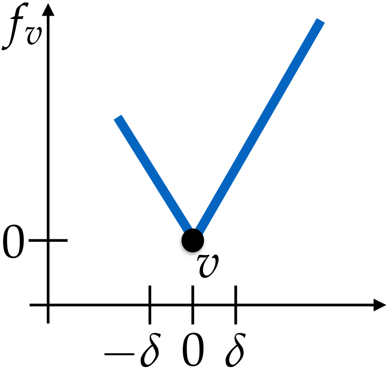
(a) The rotated and translated graph of the neighborhood of a vertex of a polygon.

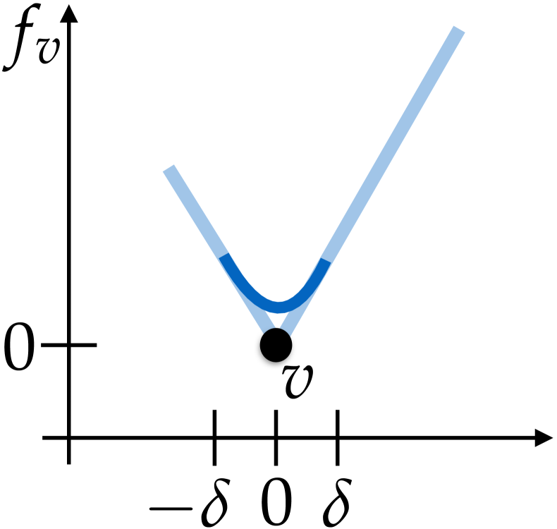
(b) The smoothed vertex of the graph $f_{v}$.

Fig. 1: The basic configuration for smoothing around a vertex.

This gives an effective means to smooth the vertices of the polygon $\mathcal{P}$; since only a neighborhood of each vertex is changed, they can be smoothed locally and then glued together along the remaining straight edges. If the interior angle at a vertex is less than $\pi,$ then the smoothed vertex lies inside of the original polygon, whereas if it is larger than $\pi,$ then the smoothed vertex lies in the exterior.

The following simple algorithm can be used to uniformly smooth the polygon $\mathcal{P}$ with a given smooth, even function $\varphi$, with support in $[-1,1]$.

Algorithm for polygonal smoothing via convolution

1. Choose a smoothing parameter $h>0$, smaller
   than $\frac{1}{2}\min\{|v_{j}-v_{j+1}|:\>j=1,\dots,n\}$.

2. For each $j$, represent a neighborhood of the vertex $v_{j}$ as the graph of an even piecewise linear function $f_{j}$ over a support line to $\mathcal{P}$ at $v_{j}.$

3. Convolve the functions $f_{j}$ with $\varphi_{h},$ to obtain $f_{j}^{h}$.

4. Replace a neighborhood of $v_{j}$ with part of the graph of $f_{j}^{h}$ by gluing along the linear parts of the graph of $f_{j}^{h}$, which agree with the graph of $f_{j}$.

Remark. The reason to use an even linear function in Step 1 is to insure that the smoothed polygon has the same discrete symmetries as $\mathcal{P}.$

The convolution can be done efficiently via either closed-form analytic expressions (depending on the choice of kernel $\varphi$) or by high-order numerical integration using an adaptive discretization scheme of the polygon and kernel as discussed in more detail in Section 3.3. Furthermore, an adaptive smoothing algorithm can be constructed by which the width parameter $h$ is allowed to depend on the pairwise vertex spacing $|v_{j}-v_{j+1}|$.

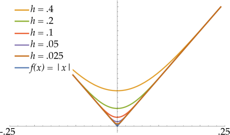
Fig. 2: A range of smoothings of a $\pi/2$ corner done by convolving a local representation with $\psi_{k}^{h},$ with $k=8$ and $h=0.025$, $0.05$, $0.1$, $0.2$, $0.4$.

3.1 Selection of smoothing kernels

To make this an effective method requires the choice of a good family of smoothing kernels. We briefly discuss the details concerning two such kernels, one compactly supported and the other numerically compactly supported. Let us first examine the family of functions $\psi_{k}(x)\in\mathcal{C}^{k-1}(\mathbb{R})$,

(3.6) $$\psi_{k}(x)=c_{k}\,(1-x^{2})^{k}\,\chi_{[-1,1]}(x),$$

where $\chi_{[a,b]}$ is the indicator function on the interval $[a,b]$. These functions should be familiar from undergraduate analysis, and are well-suited to convolutional smoothing. Here $c_{k}$ is chosen so that $\psi_{k}$ has total integral $1$. In fact,

(3.7) $$\psi_{k}(x)=\Gamma\left(k+\frac{3}{2}\right)\frac{(1-x^{2})^{k}}{\sqrt{\pi}\,\Gamma(k+1)}\,\chi_{[-1,1]}(x).$$

An example of smoothing a right-angled vertex using this kernel is shown in Figure 2.

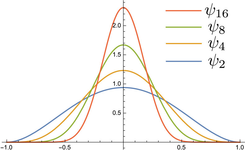
(a) Plots of $\psi_{k}$ for $k=2$, $4$, $8$, $16$.

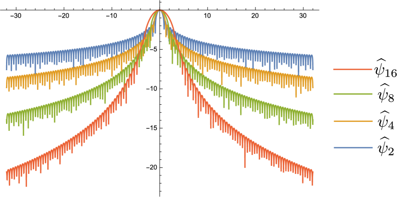
(b) $\log_{10}$ of the absolute value of the Fourier transform of the kernels $\psi_{k}$.

Fig. 3: Examples of the convolution kernels $\psi_{k}$ and their log-power spectra.

When choosing a kernel with which to perform this convolutional smoothing, it is important to choose one which is localized in both physical space and Fourier space. Post-convolution, the resulting smooth curve will then have a band-limit proportional to the product of the band-limits of the straight edges and the kernel. The lower the resulting band-limit, the more accurately the curve can be discretized with a fixed number of degrees of freedom (discretization points). The Fourier transform of the function $\psi_{k}$ is given analytically as

(3.8) $$\begin{split}\mathcal{F}\left[\psi_{k}\right](\xi)&=\widehat{\psi}_{k}(\xi)\\ &=\Gamma\left(k+\frac{3}{2}\right)\left(\frac{1}{\pi\xi}\right)^{k+\frac{1}{2}}J_{k+\frac{1}{2}}(2\pi\xi),\end{split}$$

where $J_{n}$ is the Bessel function of the first kind of order $n$ and we have chosen the convention

(3.9) $$\mathcal{F}\left[f\right](\xi)=\int_{-\infty}^{\infty}f(x)\,e^{-2\pi i\xi x}\,dx.$$

It is clear that $|\widehat{\psi}_{k}(\xi)|\leq\widehat{\psi}_{k}(0)=1$, and asymptotically for large $\xi$ these behave like:

(3.10) $$|\widehat{\psi}_{k}(\xi)|\approx\frac{e\sqrt{\pi}}{k}\left(\frac{2k}{e|\xi|}\right)^{k+1}.$$

This shows that once $|\xi|>2k/e$, the Fourier transform of $\psi_{k}$ decays quite rapidly. The Fourier transform of the scaled function satisfies

(3.11) $$\mathcal{F}\left[\frac{1}{h}\psi_{k}\left(\frac{x}{h}\right)\right](\xi)=\mathcal{F}\left[\psi_{k,h}(x)\right](\xi)=\widehat{\psi}_{k}(h\xi),$$

from which it follows that using frequencies a bit larger than $\mathcal{O}(2k/eh)$ should suffice. Graphs of the Fourier transforms of $\{\psi_{4},\,\psi_{8},\,\psi_{12},\,\psi_{16}\}$ are shown in Figure 3. Figure 4 shows multiple smoothings of regular polygons convolved with the kernel $\psi^{h}_{k}$ for various values of $h$. Note that the smoothings are nested inside one another for various values of $h$, with the more interior smoothings corresponding to larger values of $h$.

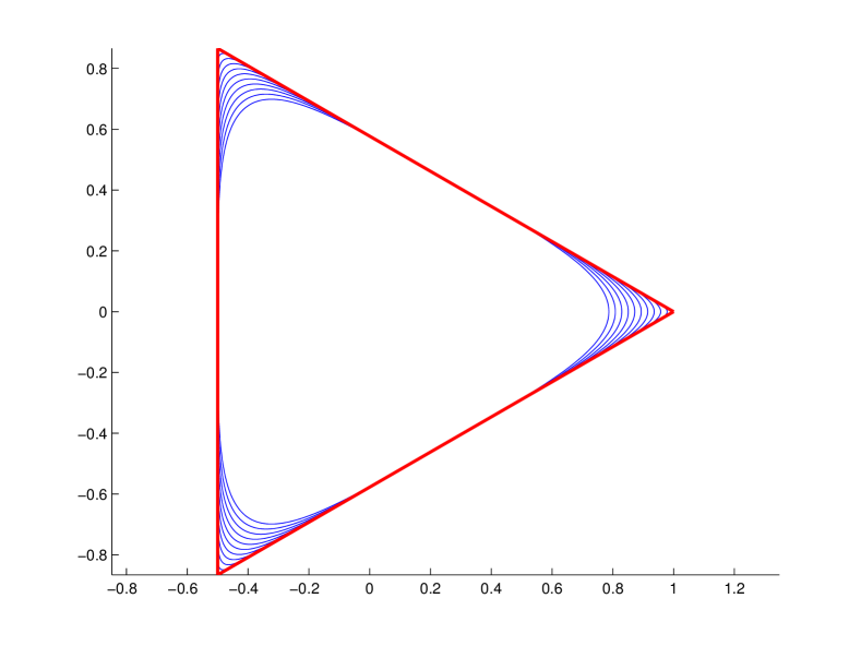
(a) Several smoothings of a triangle.

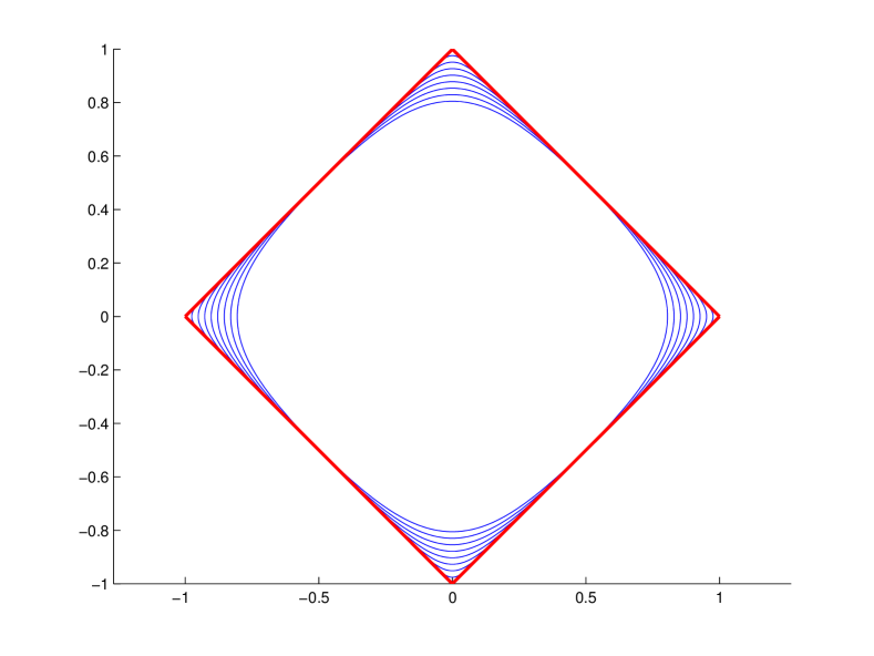
(b) Several smoothings of a square.

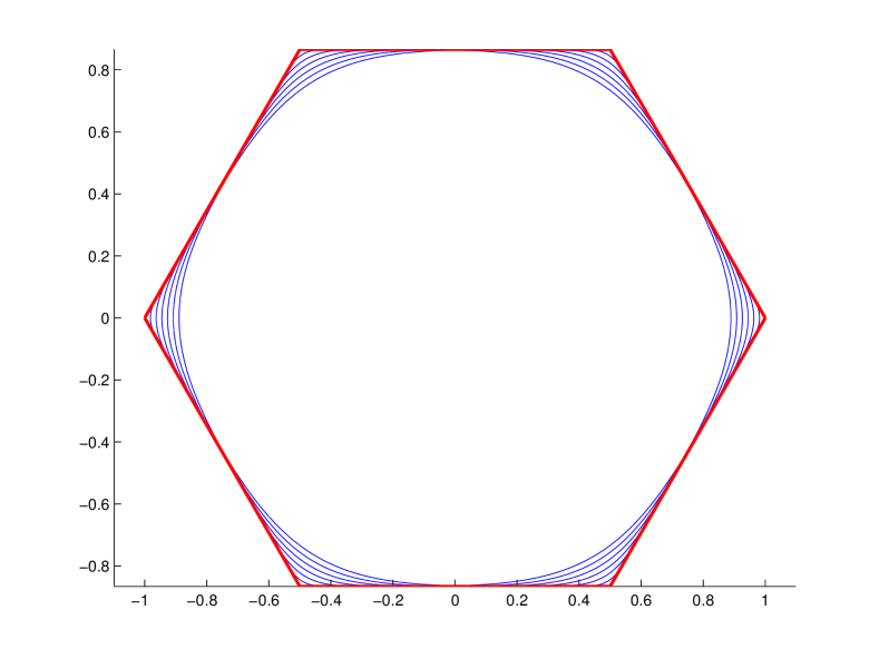
(c) Several smoothings of a hexagon.

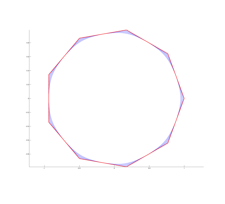
(d) Several smoothings of a nonagon.

Fig. 4: Convolutional smoothings of regular polygons.

The kernel $\psi_{k}$ in equation (3.6) is convenient to use for our purposes because of its explicit compactness. However, if we are concerned with the support in the Fourier domain of $\widehat{\psi}_{k}$ (i.e. the band-limit of $\psi_{k}$, and therefore the band-limit of the smoothed geometry), we may wish to choose a kernel with somewhat more optimal uncertainty properties, the Gaussian:

(3.12) $$\begin{split}\phi(x)&=\frac{1}{\sqrt{2\pi}}e^{-x^{2}/2},\\ \widehat{\phi}(\xi)&=e^{-2\pi^{2}x^{2}}.\end{split}$$

The kernel $\phi$ is not analytically compactly supported, however, it is numerically compactly supported. By this we mean that for any $\epsilon>0$ we can find a threshold $x_{\epsilon}>0$ such that for any $|x|>x_{\epsilon}$, $\phi(x)<\epsilon$. This, coupled with the integrability of $\phi$, allows us to choose a width parameter $h$ such that outside of a neighborhood of a vertex, the resulting smoothed geometry differs pointwise from a straight line segment by at most $\epsilon$. Furthermore, if the neighborhood of a vertex is represented as the graph of a function $f$, the convolution of $f$ with the Gaussian can be done analytically. Indeed, a symmetric $f$ will be of the form $f(x)=a|x|+b$, for some parameters $a$, $b$, and if we denote a scaled version of the Gaussian by $\phi_{h}$, then

(3.13) $$\left[\phi_{h}*f\right](x)=ax\,\text{erf}\left(\frac{x}{\sqrt{2}h}\right)+b+\sqrt{\frac{2}{\pi}}\,ah\,e^{-x^{2}/2h^{2}},$$

where erf is the error function. Clearly, for any $\epsilon>0$, there is a sufficiently large $x_{\epsilon}$ such that $|\phi_{h}*f-f|<\epsilon$ for all $|x|>x_{\epsilon}$. In the following numerical experiments, we set $\epsilon\approx 10^{-15}$ such that smoothing calculations are done to nearly machine precision. It should be noted that the choice of $\epsilon$ is independent of the choice of $h$. The value of $\epsilon$ determines the size of $|\phi_{h}(h)|$.

3.2 Discretization of the smoothing

We first discretize a smoothed geometry with a specified value of $h$ (depending on the particular polygon) using polynomial panels described by $16$ Gauss-Legendre interpolation nodes (samples of values and derivatives are obtained numerically via adaptive discretization). Each panel is resolved when the corresponding Legendre polynomial coefficients (and those of the arclength function) of an oversampled discretization are below some threshold, set to $10^{-10}$ in all cases. Obtaining higher precision is straightforward, and merely a matter of further refinement. We are mainly concerned with rough convergence on sub-wavelength rounded geometries. See Figure 5 for a picture of the discretization using Gauss-Legendre nodes on each panel, as well as a diagram of the smoothing kernel and corner.

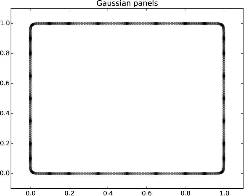
(a) The total geometry.

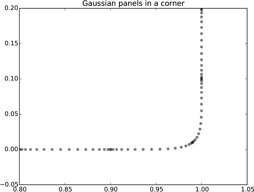
(b) A corner of the geometry.

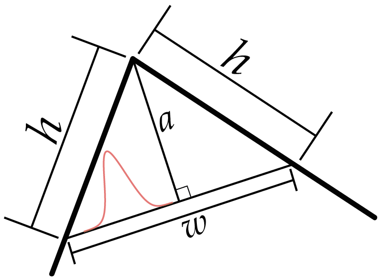
(c) Kernel arrangement.

Fig. 5: Smoothed polygon as sampled using Gauss-Legendre nodes.

Outside of a distance $h$ from the corner along an edge, the boundary contains straight edges which can be directly described using linear polynomial parameterizations. Inside a distance $h$ from the corner, we insert (via translation and rotation) an adaptive panel-based discretization of the rounded function:

(3.14) $$f_{\delta}(x)=\int_{-\infty}^{\infty}\phi_{\delta}(t)\,\left(a-\frac{a}{w/2}|t|\right)\,dt,\qquad\text{for }x\in(-w/2,w/2),$$

where for $\epsilon>0$, $\delta=\delta(w)$ is chosen such that $f_{\delta}$ matches the original polygon to precision $\epsilon$. Figure 5 depicts the lengths $a$, $w$, and $h$. It is the curve $f_{\delta}$ that is adaptively discretized so that its value, first derivative, and arclength functions are accurate to an absolute precision $\epsilon$ [52]. In all examples, $\phi_{\delta}$ is the Gaussian kernel, and the explicit convolution is given in equation (3.13). In one final pre-processing step of the geometry, further refinement takes place until all neighboring panels differ in arclength by at most a factor of two and no panel is larger than $2\lambda$, where $\lambda$ is the wavelength inherent to the problem. Using the resulting discretization nodes $\{\boldsymbol{x}_{i}\}$, we discretize the relevant integral equation (as in the next section) using the $\mathcal{L}_{2}$-weighted Nyström method. This discretization scheme, used in conjunction with high-order quadratures for weakly-singular kernels, ensures the convergence of potentials for both the Dirichlet and Neumann scattering problems in corner geometries.

We solve the linear system resulting from the Nyström discretization of the continuous integral equation directly using the LAPACK implementation of $LU$-factorization. All numerical experiments are implemented in Fortran 90 and run using the Intel Fortran Compiler with MKL libraries. Entries in the discretized matrix corresponding to source-target pairs that reside on the same panel or on neighboring panels are determined using generalized Gaussian quadratures for logarithmically singular kernels [11]. Entries corresponding to source-target pairs that reside on non-neighboring panels are obtained from the $16$-point Gaussian quadrature rule corresponding to unit weight (the Legendre polynomial case).

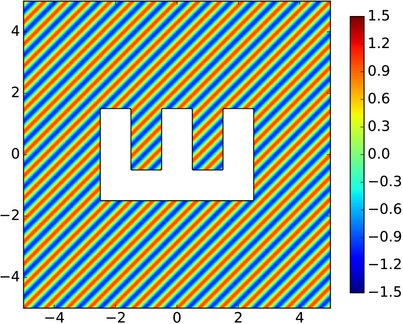
(a) The incoming field.

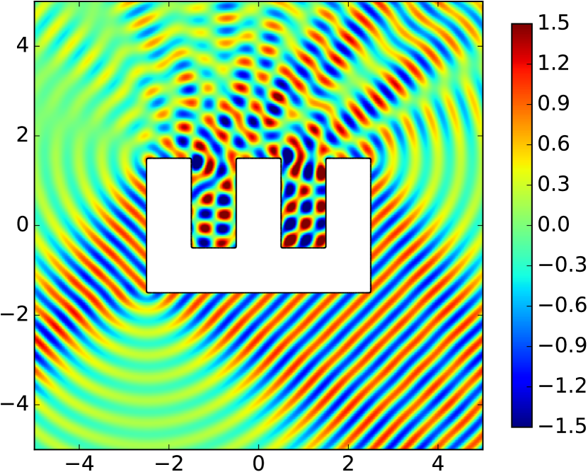
(b) The scattered field.

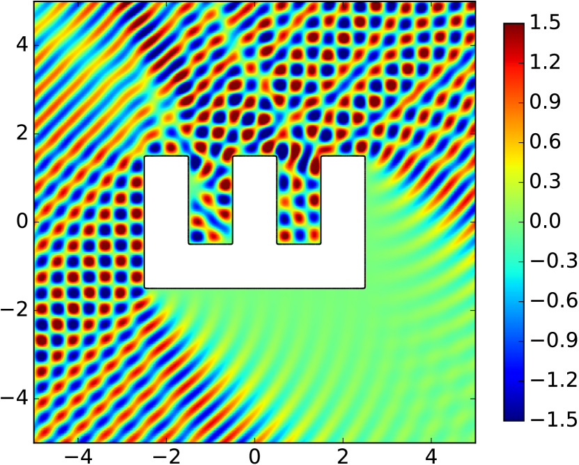
(c) The total field.

Fig. 6: Example exterior sound-soft (Dirichlet) scattering problem. The real part of all fields is shown. The angle of incident plane wave is $\phi=-\pi/4$.

3.3 Scattering from smoothed polygons: Sound-soft

We now turn our attention to numerical experiments pertaining to the scattering of acoustic waves from smoothed polygons. In this section, we study exterior Helmholtz scattering problems for Dirichlet boundary conditions; in the following section, we address the analogous Neumann problem. In the case of Dirichlet boundary conditions (corresponding to the case of a sound-soft scatterer), we have the following boundary value problem:

(3.15) $$\begin{split}(\Delta+k^{2})u^{tot}&=0\qquad\text{in }\mathbb{R}^{2}\setminus\Omega,\\ u^{tot}&=0\qquad\text{on }\Gamma=\partial\Omega,\end{split}$$

along with suitable radiation conditions at infinity. Representing the scattered solution $u$ using a combined-field potential [26],

(3.16) $$u=\left(\mathcal{S}_{k}+i\left(k\alpha+\beta\right)\mathcal{D}_{k}\right)\sigma,$$

we have the following second-kind integral equation along $\Gamma$ for the density $\sigma$:

(3.17) $$\frac{\sigma}{2}+\left(\mathcal{S}_{k}+i\left(k\alpha+\beta\right)\mathcal{D}_{k}\right)\sigma=-u^{inc}\qquad\text{on }\Gamma,$$

where $\mathcal{S}_{k}$ and $\mathcal{D}_{k}$ are interpreted in their on-surface limiting sense. We have set $\alpha=1.2$ and $\beta=0.8$ in all examples. The scattered field is then calculated at all exterior volume locations using standard Gaussian quadrature for polynomials and the fast multipole method for the two-dimensional Helmholtz equation [30]. More accurate near-surface evaluation could be obtained using the methods of [35] or [43, 49].

The following simulations are obtained from driving the scattering problem by setting $u^{inc}$ to be a two-dimensional plane-wave, traveling in the direction of the angle $\phi$:

(3.18) $$u_{\phi}^{inc}(\boldsymbol{x})=e^{ik(x\cos\phi+y\sin\phi)}.$$

It is easy to see that $u^{inc}$ satisfies the free-space Helmholtz equation, but not the Sommerfeld radiation condition. See Figure 6 for depiction of an incoming plane wave $u_{-\pi/4}^{inc}$, scattered field $u$, and total field $u^{tot}$ with Dirichlet boundary conditions. In this example, $k=12.43+i10^{-5}$, corresponding to a wavelength of $\lambda=2\pi/\operatorname{Re}{k}\approx 0.505$. The accuracy of the integral equation solver is tested by calculating the error in the potential when compared to a known solution obtained from placing a fundamental source in the interior of the object. I.e., we solve a test problem:

(3.19) $$(\Delta+k^{2})u =0 \text{in }\mathbb{R}^{2}\setminus\Omega,$$

$$u =g_{k}(\cdot,\boldsymbol{x}_{0}) \text{on }\Gamma,$$

where $\boldsymbol{x}_{0}$ is placed near the center of the object. The potential $u$ is then compared with the exact solution $g_{k}(\cdot,\boldsymbol{x}_{0})$ at test points placed on a circle some distance away from the scatterer.

We study the effect of the corner rounding by examining what is referred to as the sonar cross section (SCS) of the object $\Omega$. Usually, this function is given in terms of the far-field behavior of the scattered field based on large-$\boldsymbol{x}$ asymptotics of $H^{(1)}_{0}$:

(3.20) $$u^{far}(\boldsymbol{x})=\sqrt{\frac{1}{8\pi k}}\frac{e^{ik|\boldsymbol{x}|}}{\sqrt{|\boldsymbol{x}|}}e^{i\pi/4}\int_{\Gamma}e^{-ik\hat{\boldsymbol{r}}\cdot\boldsymbol{y}}\,\sigma(\boldsymbol{y})\,ds(\boldsymbol{y}),$$

where $\hat{\boldsymbol{r}}=\boldsymbol{x}/|\boldsymbol{x}|$. The far-field signature is often used in inverse obstacle scattering problems where measurement noise is frequently the dominant component anyway [21].

However, in our case, we have direct access to the scattered field at any observation point. We can thereby evaluate near-field functions at varying radii from the scatterer:

(3.21) $$u^{near}_{d}(\theta) =\int_{\Gamma}g_{k}(\boldsymbol{d},\boldsymbol{y})\,\sigma(\boldsymbol{y})\,ds(\boldsymbol{y}),$$

$$\boldsymbol{d} =\boldsymbol{c}+d\cos\theta\,\boldsymbol{i}+d\sin\theta\,\boldsymbol{j},$$

where we denote the scattered field at a distance $d$ from the centroid $\boldsymbol{c}$ of $\Omega$. The vectors $\boldsymbol{i}$, $\boldsymbol{j}$ are the unit vectors in the $x$, $y$ directions, respectively. There are two types of cross sections that are usually computed: mono-static and bi-static. Mono-static cross sections characterize the scatterer in terms of the intensity of the backscatter in the same direction as the incoming wave. In particular, we calculate $u^{near}_{d}$ at a single value of $\theta$ corresponding to the opposite angle of propagation of the incoming plane wave $u^{inc}_{-\theta}$. If the mono-static cross section is sampled at $m$ angles, this requires solving $m$ separate scattering problems.

On the other hand, the bi-static cross section contains intensities of the scattered field for a fixed angle of incident plane wave. Figure 7 shows sample mono-static and bi-static cross sections for the scattering problem depicted in Figure 6, each captured at a distance of $d=10\approx 20\lambda$ from the origin. The angle of incidence for the bi-static case was $\theta=-\pi/4$. In each case, the cross section is plotted on a polar grid in decibels:

(3.22) $$\mathcal{C}(\theta)=10\log_{10}\left(|u(\theta)|\right).$$

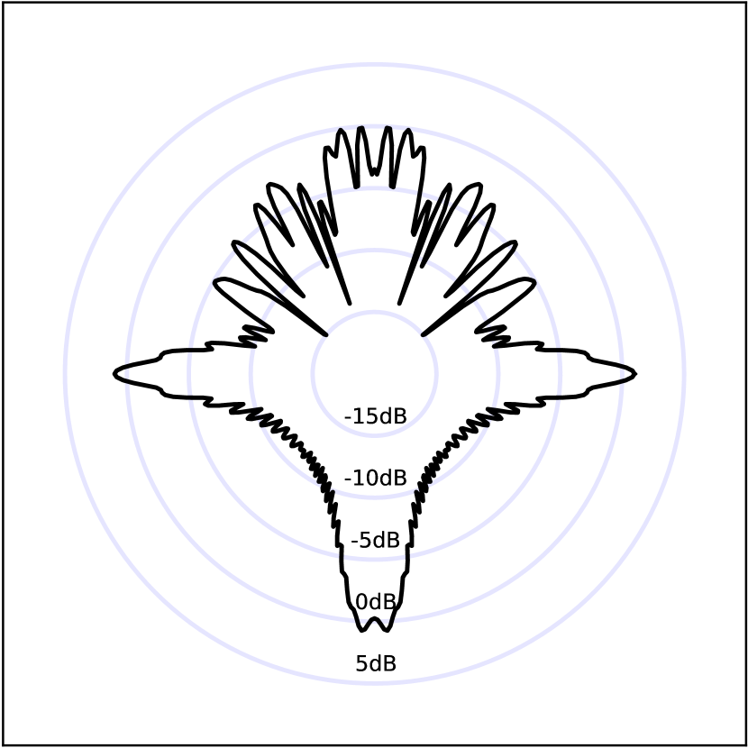
(a) The mono-static cross section.

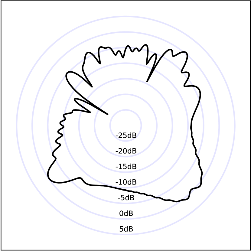
(b) The bi-static cross section.

Fig. 7: Example mono-static and bi-static cross sections for the Dirichlet problem corresponding to the geometry in Figure 6, captured at approximately $20\lambda$ from the origin. The absolute value of the scattered field is plotted on a $\log_{10}$ scale.

As the size of the region that is rounded near the corners is decreased, to below sub-wavelength, we see a convergence of the cross sections. Figure 8 shows a plot of several bi-static and mono-static cross sections for the same object (that in Figure 6). Here, we have increased the wave number to $k=54.32+i10^{-5}$ to allow for a larger dynamic range of rounding widths. This value of $k$ corresponds to a wavelength of $\lambda\approx 0.12$. The cross section is evaluated on a disc of radius $15\approx 125\lambda$ centered at the origin.

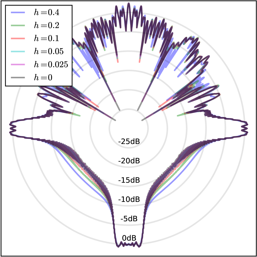
(a) Several mono-static cross sections.

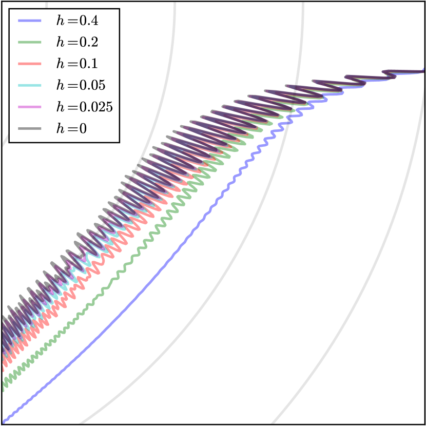
(b) Details of several mono-static cross sections.

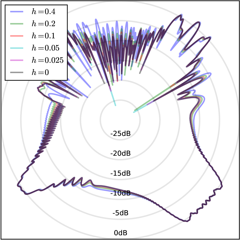
(c) Several bi-static cross sections.

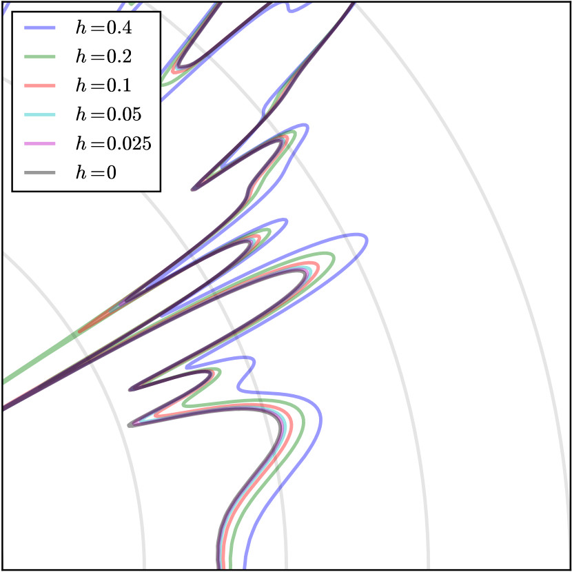
(d) Details of several bi-static cross sections.

Fig. 8: Example mono-static and bi-static cross sections for the Dirichlet problem corresponding to several roundings of the geometry in Figure 6, captured on a disc of radius $15\approx 125\lambda$ from the origin. The absolute value of the scattered field is plotted on a decibel $=10\log_{10}$ scale.

The obvious question to ask is how close these solutions are to the solution in the case of scattering from an exact polygon with corners. Results of this experiment are shown in Figures LABEL:fig_regress, LABEL:fig_diffs, LABEL:fig_diffs_big, and LABEL:fig_triangle. Convergence results of the far-field and moderately near-field bi-static cross sections are reported in Tables LABEL:tab_comb_54, LABEL:tab_comb_6, LABEL:tab_triangle52 and LABEL:tab_triangle7. Near-field convergence is given in Table LABEL:tab_comb_near. In each case, the order of convergence of the scattered field is commensurate with the scale of the rounding.

The errors in the value of the potential converge at a rate of roughly first-order with respect to the rounding parameter. Slightly faster convergence is actually observed, which may be due to the high accuracy of the rounding and the smoothing effects of the layer potential representation. We are currently investigating this phenomena. It is worth pointing out that in Figure LABEL:fig_diffs there are no correct digits in the solution (in a relative sense) until the rounding is performed on a scale roughly equal to the wavelength of the solution. The exact solution ($h=0.0$) was calculated by dyadic refinement of the edges of the polygon near the corners to a scale of $10^{-10}$. The resulting integral equation was solved using an $\mathcal{L}_{2}$ weighting scheme, as described in [7].

3.4 Scattering from smoothed polygons: Sound-hard

We now present results corresponding to the sound-hard scattering problem, i.e. the exterior Neumann problem for the Helmholtz equation:

(3.23) $$\begin{split}(\Delta+k^{2})u^{tot}&=0\qquad\text{in }\mathbb{R}^{2}\setminus\Omega,\\ \frac{u^{tot}}{\partial n}&=0\qquad\text{on }\Gamma=\partial\Omega,\end{split}$$

along with suitable radiation conditions at infinity. Representing the scattered solution $u$ using a single-layer potential:

(3.24) $$u=\mathcal{S}_{k}\sigma,$$

we have the following second-kind integral equation along $\Gamma$ for the density $\sigma$:

(3.25) $$-\frac{\sigma}{2}+\mathcal{S}_{k}^{\prime}\sigma=-\frac{\partial u^{inc}}{\partial n}\qquad\text{on }\Gamma,$$

where $\mathcal{S}_{k}^{\prime}=\partial\mathcal{S}_{k}/\partial n$ and is interpreted suitably as an on-surface limit. As before, our reference solver for the true corner problem follows the method detailed in [7].

We also recall that using representation (3.24) may yield spurious resonance in the resulting integral equation for values of $k$ which correspond to eigenvalues of the interior Laplace Dirichlet problem. For simplicity we have chosen $k$ to avoid these values. Well-conditioned combined-field representations exist which are invertible for all values of $k$ with $\operatorname{Im}{k}\geq 0$, but they involve the composition of layer potentials, as in (2.9), not merely the summation [21]. After solving (3.25), we evaluate the scattered field as in the previous section, using the fast multipole method for the two-dimensional Helmholtz equation and standard Gaussian quadrature.

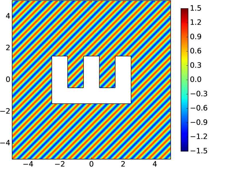
(a) The incoming field.

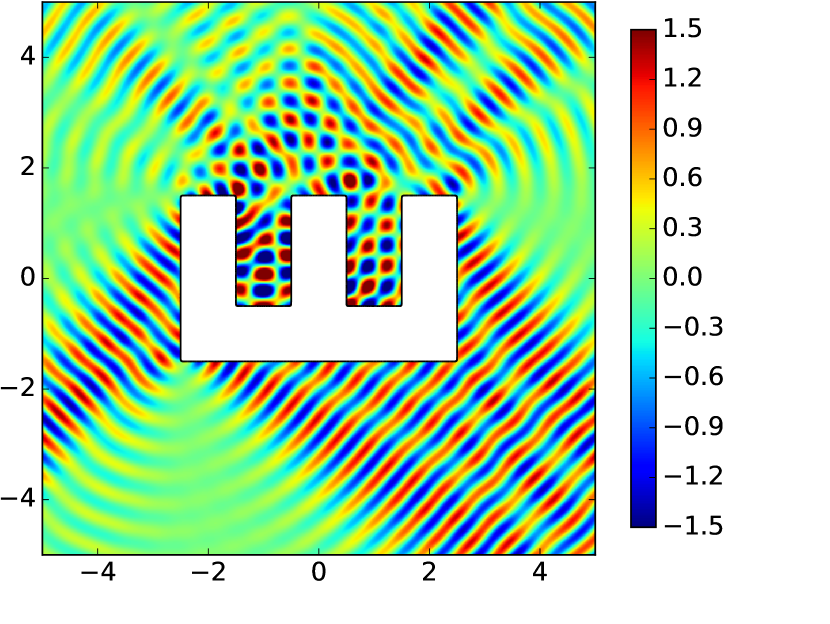
(b) The scattered field.

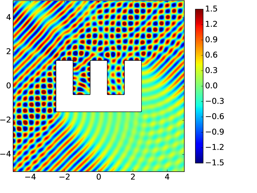
(c) The total field.

Fig. 9: Example exterior sound-hard (Neumann) scattering problem for $k=12.43+i10^{-5}$. The real part of all fields are shown. The angle of the incident plane wave is $\phi=-\pi/4$.

The following simulations are obtained from driving the scattering problem by setting $u^{inc}$ to be a two-dimensional plane-wave, as before, traveling in the direction of the angle $\phi$:

(3.26) $$u_{\phi}^{inc}(\boldsymbol{x})=e^{ik(x\cos\phi+y\sin\phi)}.$$

See Figure 9 for a depiction of an incoming plane wave $u_{-\pi/4}^{inc}$, scattered field $u$, and total field $u^{tot}$ with Neumann boundary conditions. In this example, $k=12.43+i10^{-5}$, corresponding to a wavelength of $\lambda=2\pi/\operatorname{Re}{k}\approx 0.505$.

The accuracy of the integral equation solver is tested, as before in (3.19), by comparison with a known test solution. In order to study the effect of corner rounding for the Neumann problem, we reproduce several of the experiments performed in the Dirichlet case. In particular, we compare the bi-static SCS of the true corner problem with that from successive roundings. See Figures LABEL:fig_diffs_neumann, LABEL:fig_neu_triangle, and LABEL:fig_neumann_regress for plots of Neumann solutions and convergence results.

As in the Dirichlet case, as the size of the region that is rounded near the corners is decreased, to below sub-wavelength, we see a convergence of the bi-static cross section of roughly first-order. We simulated the Neumann problem at the same frequencies as in the Dirichlet case for comparison.

3.5 Extension to piecewise smooth boundaries

This technique can also be extended to piecewise smooth curvilinear polygons. Since we need a variant of this idea to smooth polyhedra in $\mathbb{R}^{3},$ we pause to briefly describe it here. In short, in the neighborhood near a geometric singularity it is possible to construct a diffeomorphism to a truncated cone. The corner rounding can then be performed on the polygonal cone, and finally composed with the inverse of the diffeomorphism to smooth the original curvilinear polygon.

To this end, let $\mathcal{P}$ be a region in $\mathbb{R}$ whose boundary is composed of a finite collection of smoothly embedded arcs, $\{\gamma_{j}:\>j=1,\dots,n\}$ meeting at points

(3.27) $$v_{j}=\gamma_{j}\cap\gamma_{j+1}$$

and angles $\{0<\theta_{j}<2\pi\}.$ We let $\gamma_{n+1}$ denote a second copy of $\gamma_{1}.$ We are excluding the case of a cusp, i.e. $\theta_{j}=2\pi.$

Once again the idea is to change only a small neighborhood each vertex. We define (in complex notation) the planar regions

(3.28) $$W_{j} =\{z:0\leq\arg z\leq\theta_{j}\text{ and }|z|<1\}, \text{if }\theta_{j}<\pi,$$

$$W_{j} =\{z:0\leq\arg z\leq 2\pi-\theta_{j}\text{ and }|z|<1\}, \text{if }\theta_{j}>\pi.$$

Suppose that for each $j$ for which $\theta_{j}<\pi$ we can find a diffeomorphism $\psi_{j}$ from $W_{j}$ to a neighborhood of $v_{j}$ in $\mathcal{P},$ which carries:

(3.29) $$0 \to v_{j},$$

$$\{z:\arg z=0\}\cap\partial W_{j} \to\text{ a ray in }\gamma_{j},$$

$$\{z:\arg z=\theta_{j}\}\cap\partial W_{j} \to\text{ a ray in }\gamma_{j+1}.$$

If $\theta_{j}>\pi,$ then $\psi_{j}$ is defined from a neighborhood of the vertex in $W_{j}$ to a neighborhood of $v_{j}$ in $\overline{\mathcal{P}^{c}},$ with the boundary correspondence as before. Conformal mapping provides one effective method to define such maps. Other, more elementary techniques are also available. One such method, which works for regions with convex boundaries, is described in Section 6.

For each $h>0$ we define $W_{j}^{h}$ as the regions obtain by smoothing the vertex of $W_{j}$ at $0$ as described above. For small $h,$ we have $W_{j}^{h}\subset W_{j},$ and the boundaries of $W_{j}^{h}$ and $W_{j}$ coincide outside of a small neighborhood of $0.$ Thus, for small enough $r,$ the image $\psi_{j}(\partial W_{j}^{h}\setminus B_{r}(0))$ lies along the boundary of $\mathcal{P}$ outside a small neighborhood of $v_{j}.$ Hence the image $\psi_{j}(\partial W_{j}^{h})$ defines a smoothing of the vertex at $v_{j}.$ This procedure is done locally in a small neighborhood of each vertex, allowing one to smooth the vertices while leaving as much of the remainder of the boundary of $\mathcal{P}$ fixed as desired.

4 Polyhedra in three dimensions

In this section we describe several methods for smoothing piecewise smooth boundaries of regions in $\mathbb{R}^{3}$. In Section 4.1 we describe a special class of polyhedra, 3-regular Hamiltonian polyhedra, whose boundaries can be smoothed using the method described above with a parameter. In fact, all convex polyhedra, and many non-convex polyhedra can be smoothed this way, but the results are often not-optimal. In Section 4.2 we show that by modifying a polyhedron in a small neighborhood of its vertices one can obtain a 3-regular, Hamiltonian polyhedron. Hence it can be smoothed using the method given in Section 4.1. This leads to a smoothed boundary that agrees with the original polyhedron outside a small neighborhood of the original edges and vertices. Unfortunately, the smoothed polyhedron will also contain open subsets of translated support planes of the vertices. This is both unsightly and can produced a dramatically enhanced scattered wave in the direction normal to the plane. A more robust approach is described in Section 4.3.

4.1 3-Regular Hamiltonian Polyhedra

There is a special collection of polyhedra in $\mathbb{R}^{3}$ whose edges and vertices can be smoothed using only what might be called the two-dimensional method with parameter. We first define this class:

Definition 2.

Let $P$ be a polyhedron in $\mathbb{R}^{3},$ and $G_{P}$ the graph defined by its edges. $P$ is 3-regular if every vertex is the intersection of three faces, or, equivalently, if $G_{P}$ is a 3-regular graph. It is Hamiltonian if there is a finite collection of disjoint cycles $\{C_{1},\dots,C_{l}\}\subset G_{P}$ so that every vertex belongs to exactly one of these cycles.

It turns out that not every 3-regular polyhedron is Hamiltonian, and when one is, the problem of finding these cycles is not generally solvable in polynomial time. On the other hand, all 3-regular Platonic solids (tetrahedron, cube, and dodecahedron) are Hamiltonian, as well as many examples that arise in practice. As this class of polyhedra can be smoothed by smoothing only edges, we take a moment to describe the procedure.

Let $P$ be a 3-regular Hamiltonian polyhedron, with $\mathcal{C}=\{C_{1},\dots,C_{l}\}$ a collection of disjoint cycles exhausting the vertices. Let $\mathcal{E}=\{e_{1},\dots,e_{m}\}$ be the edges of $G_{P}$ that are not contained in any cycle. Because the graph is 3-regular, we know that every vertex in $G_{P}$ lies on exactly one of these edges. Moreover the edges in $\mathcal{E}$ are disjoint.

To smooth $P$ we first smooth the corners that lie along the edges in $\mathcal{E}$ (using the two-dimensional method described earlier). It is easy to see that every edge $e_{j}$ lies in the intersection of two planes $\{\pi_{j_{1}},\pi_{j_{2}}\}.$ Let $\pi_{j_{3}}$ be a plane orthogonal to the line $\ell_{j}=\pi_{j_{1}}\cap\pi_{j_{2}}$, and $\omega_{j}=(\varphi,\theta)\in S^{2}$ be the direction of $\ell_{j}$. Finally let $\gamma_{j}$ denote the component of $(\pi_{j_{1}}\cup\pi_{j_{2}})\cap\pi_{j_{3}}$ so that a neighborhood of $e_{j}$ in $P$ lies inside the corner

(4.1) $$K_{j}=\{q+t\omega_{j}:\>q\in\gamma_{j}\text{ and }t\in\mathbb{R}\}.$$

If $\gamma^{\prime}_{j}$ is a smoothing of this curve, as defined in the previous section, then

(4.2) $$K^{\prime}_{j}=\{q+t\omega_{j}:\>q\in\gamma^{\prime}_{j}\text{ and }t\in\mathbb{R}\}$$

is a smoothing of the corner. If the rounding of $\gamma_{j}$ is done close enough to the vertex, then we can smoothly replace a neighborhood of $e_{j}$ in $P$ with its smoothed version in $K^{\prime}_{j}$ by simply intersecting the interior of the region bounded by $K^{\prime}_{j}$ with $P.$ Away from the smoothed edge, $K_{j}^{\prime}$ is still a union of planar regions which can be glued onto $P$, thereby replacing $e_{j}$ with a smooth transition between these planar regions.

Since the edges in $\mathcal{E}$ do not intersect, each of these smoothing operations can be done independently of the others. Let $P^{\prime}$ denote the body in $\mathbb{R}^{3}$ obtained by smoothing all of these edges. Since every vertex lies on one of the edges in $\mathcal{E}$, the cycles on $P$ are replaced by cycles $\mathcal{C}^{\prime}=\{C^{\prime}_{1},\dots,C^{\prime}_{l}\}$ on $P^{\prime}$ that are smooth non-intersecting curves. That is to say, every vertex has been smoothed. The boundary of the body $P^{\prime}$ is a comprised of bounded smooth surfaces, which are mostly planar regions. These surfaces are bounded by smooth, disjoint, closed curves, along which these surfaces meet. All that remains is to smooth these curves of intersection.

To that end we now define a diffeomorphism from a standard model onto a neighborhood of $C_{j}^{\prime}$. We smooth the standard model and use this map to glue the result into $P^{\prime}$. Let $c_{j}:[0,L_{j}]\to P^{\prime}$ be an arclength parameterization of $C_{j}^{\prime}$. The unit vector field $T_{j}(t)=\partial_{t}c_{j}$ is tangent to $C_{j}^{\prime}$. Two smooth surfaces $S_{1j}$ and $S_{2j}$ meet, transversely, along this curve. Let $N_{ij}(t)$ be the unit vector normal to $T_{j}(t)$ lying along $S_{ij},$ $i=1,2$. Let $\pi_{j}(t)$ denote the plane through $c_{j}(t)$ spanned by $\{N_{1j}(t),N_{2j}(t)\}$.

For $\epsilon>0$, let $U_{j\epsilon}$ denote the $\epsilon$-neighborhood of $C_{j}^{\prime}$. There is a radius $\epsilon>0$ so that these planes $\{\pi_{j}(t):\>t\in[0,L_{j}]\}$ define a foliation of $U_{j\epsilon}.$ This follows from the inverse function theorem and the compactness of the curve. We define a map from $V_{j\delta}=[0,L_{j})\times(-\delta,\delta)\times(-\delta,\delta)$ into a neighborhood of $C_{j}^{\prime}$ by letting

(4.3) $$\Phi_{j}(t,s_{1},s_{2})=c_{j}(t)+s_{1}N_{1j}(t)+s_{2}N_{2j}(t).$$

The differential of $\Phi_{j}$ at $(t,0,0)$ is given by

(4.4) $$d\Phi_{j}(t,0,0)=T_{j}(t)dt+N_{1j}(t)ds_{1}+N_{2j}(t)ds_{2},$$

which is clearly of rank three. From the inverse function theorem it now follows easily that there is an $\delta>0$ so that $\Phi_{j}\upharpoonright_{V_{j\delta}}$ is a diffeomorphism onto its image, which is a neighborhood of $C^{\prime}_{j}$ foliated by the planes $\{\pi_{j}(t)\}.$ We can continue $\Phi_{j}$ as a smooth $L_{j}$-periodic function.

We first make the assumption that $P^{\prime}\cap U_{j\epsilon}$ lies in the image of the positive orthant in the $(s_{1},s_{2})$-variables under this map. This is certainly the case if the interior angle along $C_{j}^{\prime}$ is everywhere less than $\pi$. Under this assumption it is easy to see that for an $\eta>0$ there is a set of the form $V_{j\eta}=\mathbb{R}\times[0,\eta]\times[0,\eta]$ on which $\Phi_{j}$ is a periodic-diffeomorphism. Moreover $\Phi_{j}(V_{j\eta})\subset P^{\prime}$ exhausts a neighborhood of $C^{\prime}_{j}$ in $P^{\prime}.$

We now smooth the corner $V_{j\eta}$ to obtain $V^{\prime}_{j\eta}$, where the smoothed edge lies in $V_{j\frac{\eta}{2}}.$ The image of the smoothed corner under $\Phi_{j}$ defines a smoothing of $C^{\prime}_{j}$. As these curves are disjoint, each one can be smoothed independently. We let $P^{\prime\prime}$ denote the resulting body in $\mathbb{R}^{3}.$ It is a smoothed approximation to $P.$ If the interior angle is greater than $\pi$ at every point, then we can smooth the corner by smoothing the exterior, which satisfies the hypotheses above.

We demonstrate this approach to smoothing polyhedra by smoothing a cubic torus $P$. We suppose that $P$ is oriented parallel to the standard coordinate axes. There are four cycles $\{C_{1},\ldots,C_{4}\}$, each containing four edges and parallel to the $xz$-plane. These cycles bound the faces that have non-trivial topology. For the edges not belonging to cycles, $\mathcal{E}$, we use the eight edges parallel to the $y$-axis. If the edges in $\mathcal{E}$ are smoothed, then the cross sections of $P^{\prime}$ perpendicular to the $y$-axis are smoothed squares, as shown in Figure 10.

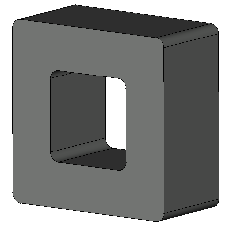
(a) Rounded edges and cycles of the cubic torus.

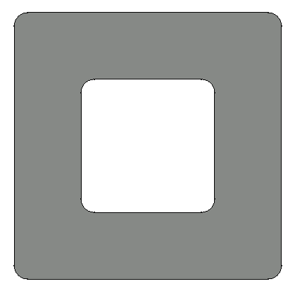
(b) Rounded edges/cycles of a face.

Fig. 10: Rounding Hamiltonian cycles of a cubic torus. Images were constructed merely for illustrative purposes only using FreeCAD.

We now smooth the remaining edges using the representation in equation (4.3) along with the smoothing of the right angle used to smooth the edges in $\mathcal{E}$. Figure 11 shows two views of the upper part of the final smoothed cubic torus. We should point out that these images were constructed using the software FreeCAD using low-order fillet procedures, and are illustrative only. Constructing the high-order computational geometry software to carry out convolutional smoothing and subsequent high-order piecewise triangulation for polyhedra in three dimensions is an ongoing project.

4.2 Smoothing the Vertices: I

The method for smoothing edges described in the previous section can be used to smooth an arbitrary convex polyhedron in a two-step procedure. Let $\mathcal{P}$ be a convex polyhedron with faces $\mathcal{F}=\{f_{1},\dots,f_{l}\}$, edges $\mathcal{E}=\{e_{1},\dots,e_{m}\}$, and vertices $\mathcal{V}=\{v_{1},\dots,v_{n}\}$. At each vertex we choose an outward pointing support vector, $\{\boldsymbol{\nu}_{1},\dots,\boldsymbol{\nu}_{n}\}$. Suppose that the edges at the $j^{\text{th}}$ vertex join to the vertices $\{v_{k_{1}},\dots,v_{k_{p}}\}.$ A good choice for $\boldsymbol{\nu}_{j}$ is to take

(4.5) $$\boldsymbol{\nu}_{j}=\frac{1}{p}\sum_{q=1}^{p}\frac{v_{j}-v_{k_{q}}}{\|v_{j}-v_{k_{q}}\|},$$

as it will preserve whatever symmetries the original polyhedron possesses in the smoothed domain.

Given $\epsilon>0,$ we define a neighborhood $V_{\epsilon}$ of the vertices by the condition

(4.6) $$X\in V_{\epsilon}\text{ if for some }j\text{ we have }\langle X-v_{j},\boldsymbol{\nu}_{j}\rangle>-\epsilon.$$

Note that $\mathcal{P}\subset V_{0}^{c},$ and, for small $\epsilon>0$, the intersection $\partial V_{\epsilon}\cap\mathcal{P}$ is a disjoint union of small polygons lying near the vertices. See Figure 12(a). It is easy to see that the resultant polyhedron is 3-regular and Hamiltonian, with the disjoint cycles being those introduced when cutting off the vertices.

To smooth the polyhedron we first smooth the edges. An edge $e_{k}$ lies in the intersection of two faces $f_{i_{k}}\cap f^{\prime}_{i_{k}}.$ Let $\pi_{k}$ be the plane, through the midpoint of the edge, which is perpendicular to $e_{k}.$ Using the method described in Section 3 we can smooth the vertex $e_{k}\cap\pi_{k}$ of the polygon defined by the intersection of $\pi_{k}$ with $\mathcal{P}.$ By parallel translating this smoothed vertex along the edge, we can replace a neighborhood of the edge $e_{k}$ by a smooth surface joining the plane containing $f_{i_{k}}$ to the plane containing $f^{\prime}_{i_{k}}.$ With $h>0$ the smoothing parameter from Section 3, we let $\mathcal{P}_{h}$ denote the polygon with all its edges smoothed in this manner.

Of course, near enough to a vertex, the smoothings of different edges intersect, but given $\epsilon>0$ we can choose a sufficiently small $h>0$ so that, in the set $V_{\epsilon}^{c},$ the modifications corresponding to the different edges are disjoint. With such choices, the intersection $\partial V_{\epsilon}\cap\mathcal{P}_{h}$ is a disjoint union of polygons with smoothed vertices lying in the planes

(4.7) $$\langle X-v_{j},\boldsymbol{\nu}_{j}\rangle=-\epsilon.$$

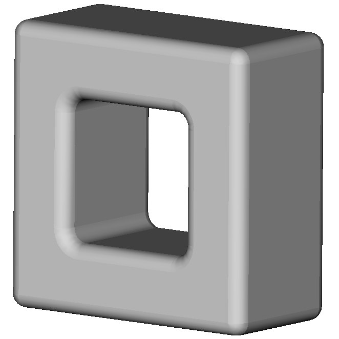
(a) Final smooth surface.

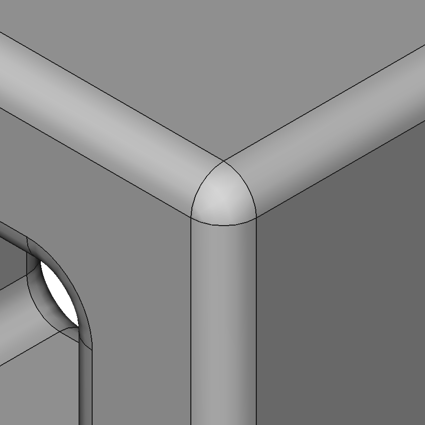
(b) Smoothed exterior corner.

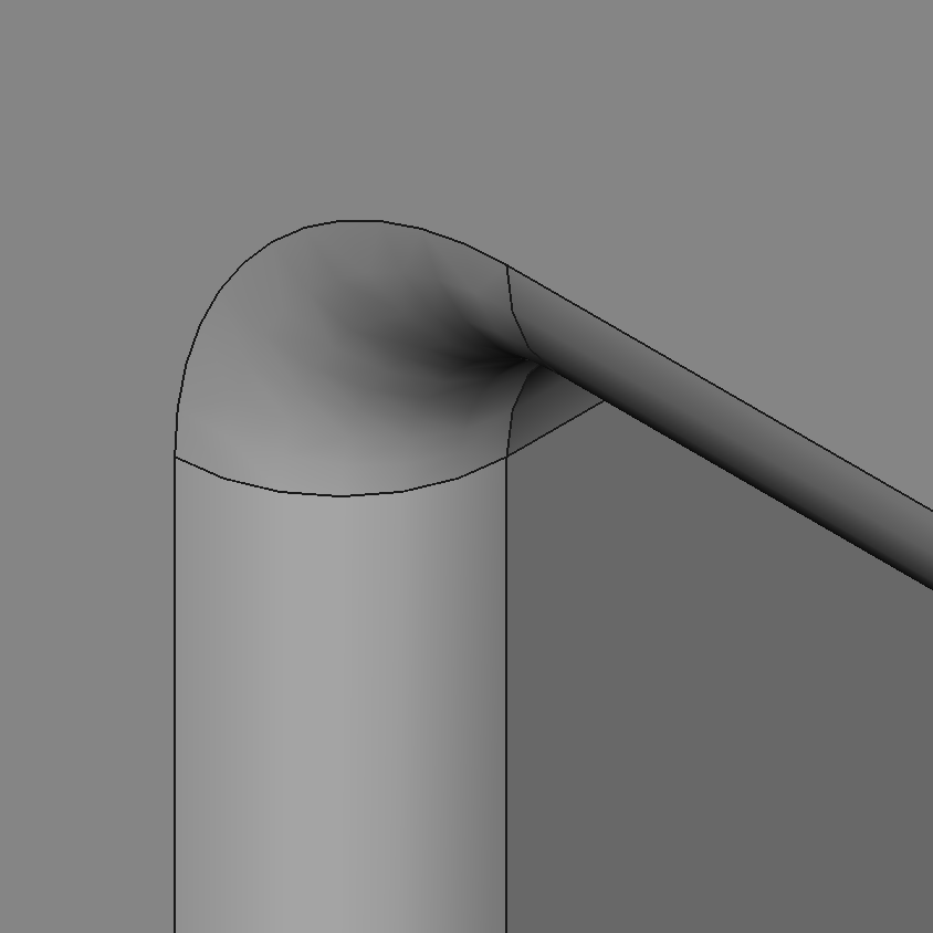
(c) Smoothed interior corner.

Fig. 11: Final rounding of Hamiltonian cycles of a cubic torus. Images were constructed merely for illustrative purposes only using FreeCAD.

Using the technique described in Section 4.1 the edges along which these smoothed polygons meet $\partial\mathcal{P}_{h}$ can be smoothed, leading to an overall smoothing of the original polyhedron. While it is clear that this can be done in an arbitrarily small neighborhood of the singular locus of $\partial\mathcal{P},$ the $j^{\text{th}}$ vertex is replaced by a smooth surface containing a open subset of the plane defined in (4.7). For applications to scattering theory this might not be desirable, as it will produce a considerable amplification of the scattered signal in this direction. In the next section we describe a method for smoothing vertices that produces a better result.

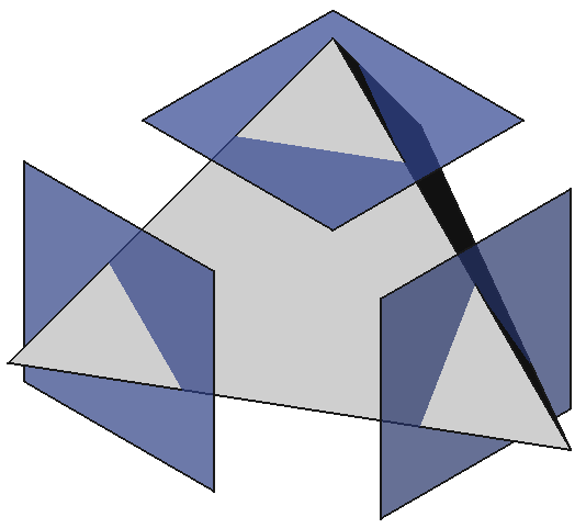
(a) The intersections of $\mathcal{P}$ with planes
$\langle X-v_{j},\boldsymbol{\nu}_{j}\rangle=-\epsilon$.

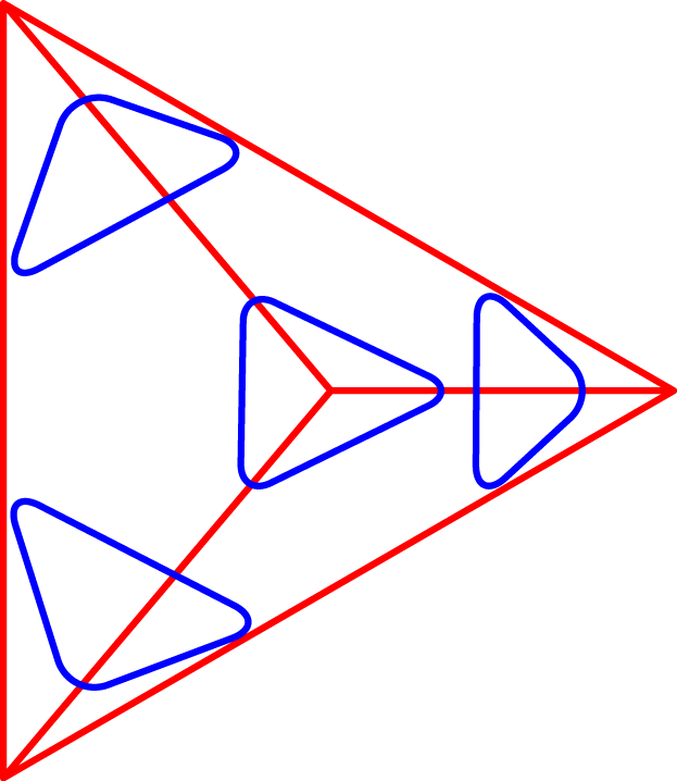
(b) View along the $z$-axis of the intersections of the smoothed edges with planes
$\langle X-v_{j},\boldsymbol{\nu}_{j}\rangle=-\epsilon$.

Fig. 12: Corner rounding of a tetrahedron. Images are for illustrative purposes only, constructed using FreeCAD.

4.3 Smoothing the Vertices, II

The second method for smoothing vertices takes as its starting point the domain $\mathcal{P}_{h}$ constructed in the previous sections by smoothing the edges (as depicted in Figure 12(b)). We assume that there is a positive $\epsilon_{0}$ so that the intersections

(4.8) $$P^{h,j}_{\epsilon_{0}}=\mathcal{P}_{h}\cap\{X:\langle X-v_{j},\boldsymbol{\nu}_{j}\rangle=-\epsilon_{0}\}$$

are disjoint smoothed polygons. With this assumption each vertex can be smoothed without reference to any other vertex. We can therefore fix a $j$ and describe the method for smoothing $\mathcal{P}$ in a neighborhood of $v_{j}.$

We let $0<\epsilon_{j}<\epsilon_{0}$ denote the infimum of the numbers so that $P^{h,j}_{\epsilon}$ is a polygon with smoothed vertices. The domain $P^{h,j}_{\epsilon_{j}}$ is a smoothed polygon, where the smoothings of two (or more) of the edges meet without any flat segment between them.

For each $\epsilon>\epsilon_{j},$ we let $\Phi_{\epsilon}$ denote a maximally smooth parameterization of $\partial P^{h,j}_{\epsilon}$ on the unit circle. That is, $\Phi_{\epsilon}$ is a map from $S^{1}$ to $\partial P^{h,j}_{\epsilon}$. Therefore, we can represent it in terms of a Fourier expansion:

(4.9) $$\Phi_{\epsilon}(\theta)=\sum_{n=-\infty}^{\infty}X_{\epsilon,n}e^{in\theta}-\epsilon\boldsymbol{\nu}_{j}.$$

The infinite sum defines a map from the unit circle to $\partial P^{h,j}_{\epsilon}$ translated to the plane $\langle X,\boldsymbol{\nu}_{j}\rangle=0.$ We adjust $\epsilon_{0}$ so that $\epsilon_{0}>4\epsilon_{j}$ for all $j.$

For each $\epsilon_{j}\leq\epsilon\leq\epsilon_{0}$ we can extend this map as a diffeomorphism from the unit disk to the smoothed polygon $P^{h,j}_{\epsilon}.$ For example, since the boundary of $P^{h,j}_{\epsilon}$ is convex, it follows from a theorem of Choquet that the harmonic extension has the desired properties:

(4.10) $$\widetilde{\Phi}_{\epsilon}(r,\theta)=\sum_{n=-\infty}^{\infty}X_{\epsilon,n}e^{in\theta}r^{|n|}-\epsilon\boldsymbol{\nu}_{j}.$$

For additional details, see the next section and [20]. The image of $\widetilde{\Phi}_{\epsilon}$ lies in the plane $\langle X-v_{j},\boldsymbol{\nu}_{j}\rangle=-\epsilon$.

To use these maps to define a smoothing we need to choose two auxiliary functions. First we choose a number $\eta_{1}$ so that $2\epsilon_{j}<\eta_{1}<\epsilon_{0}$. Next, choose a smooth, convex, increasing function $\chi(s)$ defined in $[0,\epsilon_{0}]$ so that for $s>\eta_{1}$, $\chi(s)=s$, $\chi(0)=\epsilon_{j}$, and

(4.11) $$\chi^{[m]}(0)=0\qquad\text{for }m=1,\dots,k.$$

We also choose positive numbers $r_{0}<\epsilon_{0},$ $\eta_{2}<r_{0}/2,$ and an even convex function $\psi(r)$ defined in a neighborhood of $0.$ We require

(4.12) $$\psi(r) =r \text{for }r>r_{0},$$

$$\psi(0) =\eta_{2},$$

$$\psi^{[m]}(0) =0 \text{for }m=1,\dots,k.$$

The smoothing of the neighborhood is defined as the image of $[0,\epsilon_{0}]\times S^{1}$ under the map

(4.13) $$\Psi(r,\theta):(r,\theta)\mapsto\widetilde{\Phi}_{\chi(r)}\left(\frac{r}{\psi(r)},\theta\right)-\chi(r)\boldsymbol{\nu}_{j}.$$

For $r>\max\{\eta_{1},r_{0}\}$ this map simplifies to

(4.14) $$(r,\theta)\mapsto\widetilde{\Phi}_{r}\left(1,\theta\right)-r\boldsymbol{\nu}_{j}.$$

That is to say, its image lies in the already smoothed part of $\partial\mathcal{P}_{h}$ near to $v_{j}.$ Our assumptions assure, that as function of $x=r\cos\theta$ and $y=r\sin\theta$, the map $(x,y)\mapsto\Psi(x,y)$ is at least $m-1$ times differentiable in a neighborhood of $(0,0)$ and $d\Psi(0,0)$ has rank $2$. Therefore, the image of $D_{\epsilon_{0}}(0)$ under $\Psi$ is a smooth sub-manifold of $\mathbb{R}^{3}$. The image lies in the set

(4.15) $$\langle X-v_{j},\boldsymbol{\nu}_{j}\rangle\leq-\epsilon_{j},$$

where the vector $\boldsymbol{\nu}_{j}$ is the normal vector to the smoothed vertex at the point $\Psi(0,0)$.

In describing this method for smoothing vertices, we have assumed that the original polyhedron is convex, but this is not necessary for the method to be applicable. It is merely required that each vertex $v_{j}$ has a local strict supporting plane. This means that there is a vector $\boldsymbol{\nu}_{j}$ so that if $\langle v_{j},\boldsymbol{\nu}_{j}\rangle=c_{j}$, then for some $r>0$,

(4.16) $$\mathcal{P}\cap B_{r}(v_{j})\setminus v_{j}\subset\{X:\langle X,\boldsymbol{\nu}_{j}\rangle<c_{j}\}.$$

Here $B_{r}(v)=\{X\in\mathbb{R}^{3}:|X-v|<r\}.$ The existence of a strict local support plane implies that for a range of $\epsilon>0$ the sets

(4.17) $$P^{j}_{\epsilon}=\mathcal{P}\cap\{X:\langle X-v_{j},\boldsymbol{\nu}_{j}\rangle=-\epsilon\}$$

are polygons. With this assumption we proceed as before, first smoothing the edges to produce $\mathcal{P}_{h}.$ For some $0<\epsilon_{0}<\epsilon<\epsilon_{1}$ the sets

(4.18) $$P^{h,j}_{\epsilon}=\mathcal{P}_{h}\cap\{X:\langle X-v_{j},\boldsymbol{\nu}_{j}\rangle=-\epsilon\}$$

are smoothed polygons. The method described above can easily be adapted to smooth the vertex in this case as well. The results of using this technique to smooth polyhedra are shown in Figure 13.

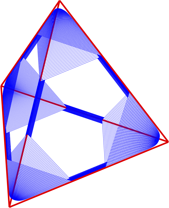
(a) A smoothed tetrahedron.

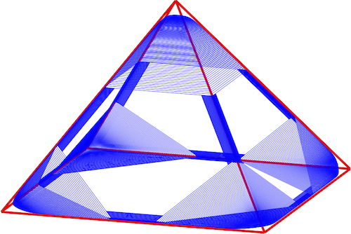
(b) A smoothed pyramid.

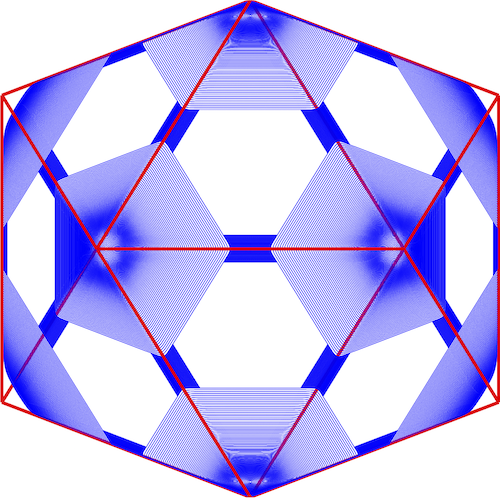
(c) A smooth icosahedron.

Fig. 13: Several smoothed polyhedra.

5 General Polyhedra

Using this general scheme of first smoothing the edges, and then using diffeomorphisms to smooth the vertices we now describe a method that suffices to smooth arbitrary globally embedded polyhedra in $\mathbb{R}^{3}.$ Let $\mathcal{P}$ be a polyhedron, by which we mean a bounded region in $\mathbb{R}^{3},$ whose boundary is a union of polygons lying in planes. We let $\{v_{j}\}$ denote the vertices of $\mathcal{P}.$ If the polyhedron has a strict local support plane at every vertex, then the method describe in Section 4.3 can be applied to produce a locally smoothed polyhedron, by first smoothing the edges and then the vertices. There are polyhedra that do not have strict local support planes at every vertex, e.g. the cubic torus does not have support planes at the inner vertices.

The method of Section 4.3 requires that near to the vertex $v_{j},$ the polyhedron is the cone over an intersection with a plane of the form

(5.1) $$\mathcal{P}\cap\{X:\langle X-v_{j},\boldsymbol{\nu}_{j}\rangle=-\epsilon\}.$$

Let $S_{r}(v)$ denote the sphere of radius $r$ centered at $v.$ A slightly more complicated method results if we instead assume that for each $j$ there is an $r_{j}>0$ so that

1. $\mathcal{P}\cap S_{r_{j}}(v_{j})$ is a connected region $R_{j}$ on $S_{r_{j}}(v_{j})$ bounded by a simple closed curve, $\gamma_{j}$,

2. $\mathcal{P}\cap B_{r_{j}}(v_{j})$ is the cone over $R_{j}$ with vertex $v_{j}$.

The curve $\gamma_{j}$ is a piecewise geodesic polygon on the sphere. A polyhedron satisfying these conditions is globally embedded. In general the region $R_{j}$ could have several connected components, a case that we do not consider further.

For sufficiently small $h>0$, we let $\mathcal{P}_{h}$ denote the result of smoothing the edges of $\mathcal{P}$ as described in Section 4.2. If $\mathcal{P}$ is globally embedded, then, at each vertex there is a range of radii $\rho_{0j}(h)<r<\rho_{1j}(h)$ so that the intersections

(5.2) $$\mathcal{P}_{h}\cap S_{r}(v_{j})$$

are regions $R_{j}(r,h)$ bounded by simple closed curves, $\gamma_{j}(r,h)$, that are smoothings of the curves $\mathcal{P}\cap S_{r}(v_{j}).$ As $h\to 0,$ it is clear that $\rho_{0j}(h)$ tends to $0$ and $\liminf_{h\to 0}\rho_{1j}(h)\geq r_{j}.$

For each $\rho_{0j}(h)<r<\rho_{1j}(h)$ we let

(5.3) $$\Phi_{r}:D_{1}(0)\longrightarrow R_{j}(r,h)$$

be a diffeomorphism from the unit disk onto the region $R_{j}(r,h).$ The maps $\{\Phi_{r}\}$ can, for example, be defined as the conformal maps from $D_{1}(0)$ to the spherical domain $R_{j}(r,h),$ normalized so that $0$ is mapped to points lying on a carefully selected curve. Using these maps we can define an analogue of the map $\Psi(r,\theta),$ defined in (4.13), so that the image of $[0,\epsilon_{0}]\times S^{1}$ under this map is a smoothed version of a neighborhood of the vertex $v_{j},$ which is joined smoothly to $\mathcal{P}_{h}.$ We leave the detailed construction of these maps to the ambitious reader.

There are also approaches to smoothing that first smooth the vertices, using the methods described above, and then interpolate these smoothings along the edges. It is very difficult to preserve convexity using this order of operations. That is why we have only described methods that first smooth the edges, and then the vertices, using a slicing approach along with families of diffeomorphisms.

This completes the description of our algorithms for smoothing polyhedra in $\mathbb{R}^{3}.$ Note that one can restrict the modifications of the original polyhedron to lie in an arbitrarily specified neighborhood of the 1-skeleton of the boundary of $P.$ One also retains considerable control on the relationship between the Gauss map of the smoothed polyhedron and that of the original, which is crucial for the behavior of scattered waves. In the final section we provide several practical methods for constructing diffeomorphisms.

6 Methods to construct diffeomorphisms

We now describe several methods to define extensions of a map from $S^{1}$ to $\Gamma,$ a Jordan curve in the plane, which are diffeomorphisms from the unit disk $D_{1}(0)$ to the region $D_{\Gamma}$ which is bounded by $\Gamma$.

6.1 Method 1

Conformal mapping provides a method that can be computationally expensive and numerically ill-conditioned (depending on the geometry) [46], but guaranteed to work in considerable generality. In particular $D_{\Gamma}$ can be a simply connected region in either a plane or a round sphere. Suppose that $f:D_{1}(0)\to D_{\Gamma}$ is a conformal diffeomorphism. If $\Gamma$ is convex, then

(6.1) $$\Gamma_{r}=\{f(re^{i\theta}):\>\theta\in[0,2\pi]\}$$

is a convex curve for every $r\in(0,1]$. If $\Gamma$ is star shaped with respect to $0$ and $f$ is normalized so that $f(0)=0$ then the curves $\{\Gamma_{r}:r\in(0,1]\}$ are star shaped. These results can be found in [48].

6.2 Method 2

There is a simple method that is guaranteed to give a diffeomorphism if $D_{\Gamma}$ lies in a plane and the initial curve $\Gamma$ is convex. A theorem of T. Rado, Kneser, and G. Choquet states that if $(u,v)$ defines a homeomorphism from the unit circle to $\Gamma$ which bounds a convex region $D_{\Gamma}$, then the harmonic extension of the coordinate functions $(U,V)$ defines a diffeomorphism from the interior of $D_{1}$ to $D_{\Gamma}$ [20]. This theorem does not require $\Gamma$ to be strictly convex or smooth.

If the boundary map is given in terms of the Fourier series

(6.2) $$\theta\mapsto\left(\sum_{j=-\infty}^{\infty}a_{j}\,e^{ij\theta},\,\sum_{j=-\infty}^{\infty}b_{j}\,e^{ij\theta}\right)$$

it follows from Choquet’s theorem that

(6.3) $$\Phi(\theta,r)=\left(\sum_{j=-\infty}^{\infty}a_{j}\,r^{|j|}e^{ij\theta},\,\sum_{j=-\infty}^{\infty}b_{j}\,r^{|j|}e^{ij\theta}\right)$$

defines a diffeomorphism from $D_{1}(0)$ onto $D_{\Gamma}.$

6.3 Method 3

If we specify a convex curve $\Gamma$ in terms of its Gauss map, that is, as the image

(6.4) $$G(\theta)=g(\theta)\,\left(\cos\theta,\sin\theta\right)+g^{\prime}(\theta)\,\left(-\sin\theta,\cos\theta\right),$$

then we can proceed as above to get a diffeomorphism. If $g$ has the Fourier representation

(6.5) $$g(\theta)=\sum_{n=-\infty}^{\infty}\beta_{n}\,e^{in\theta},$$

then we can again apply Choquet’s theorem to construct a harmonic extension, which is guaranteed to give a diffeomorphism. The map defined in (6.4) can be represented as

(6.6) $$e^{i\theta}\mapsto(g(\theta)+ig^{\prime}(\theta))e^{i\theta}.$$

Using the Fourier representation in (6.5), we see that

(6.7) $$G(\theta,r)=\sum_{n=-\infty}^{\infty}\beta_{n-1}\,(2-n)\,r^{|n|}e^{in\theta}$$

defines the harmonic extension of this map, and is therefore a diffeomorphism from $D_{1}(0)$ onto $D_{\Gamma}.$

7 Conclusions

In this paper we have presented several algorithms for modifying polygons and polyhedra into fully regularized surfaces without geometric singularities (vertices and edges). The original polygon (or polyhedron) is modified in a controllable and arbitrarily small neighborhood of its singular set. We have compared the solution to acoustic scattering problems from the original singular boundary to that obtained by smoothing the boundary at sub-wavelength scales in two dimensions. Both near- and far-field solutions converge at a rate slightly faster than first-order in the rounding parameter. Understanding this rate of convergence is an ongoing research topic in our group.

Constructing numerical codes for performing rounding in two dimensions is relatively straightforward. We presented results for the polygonal case; software implementing the rounding of vertices joining piecewise smooth curves is currently under development, requiring merely the re-parameterization of the curve near the vertex as a graph above a support line tangent to the vertex. These computations are relatively fast, efficient, and accurate to near machine precision in two dimensions.

We also introduced the analytical foundation for constructing high-order roundings of polyhedra in three dimensions. Composing various methods with diffeomorphisms near vertices allows for similar regularizations to be computed as in the two-dimensional case. Building more efficient software to perform these computations is a work in progress.

Preliminary Matlab code which performs the vertex and edge smoothing for convex polyhedra in three dimensions has been made available at:

http://gitlab.com/oneilm/rounding

If only approximate scattering solutions are required to the true problem involving geometries with corners and edges, the algorithms of this paper offers a method to obtain these results with reduced computational cost and controlled accuracy. Furthermore, the methods require nothing other than the usual quadratures for weakly-singular functions on smooth curves or surfaces. Full extensions of these smoothing algorithms to three dimensions may have a wide array of applications in high-order CAD and CAE packages, as many existing software solutions only allow for twice differentiable roundings (fillets).

Lastly, we would like to note that the algorithms presented in this paper for geometric regularization in three dimensions are only one piece of a larger effort to develop high-order scattering codes for arbitrary geometries. In three dimensions, all the numerical tools that are required to solve boundary integral equations are more expensive and more sophisticated than those in two dimensions. Merely constructing high-order Nyström-compatible quadratures for the function $1/|\boldsymbol{x}-\boldsymbol{y}|$ along triangular patches is a relatively recent result [9, 10]. Coupling these schemes with fast algorithms and high-order triangulations is under active development. Performing the analogous convergence studies for rounding in three dimensions will be reported at a later date, after the requisite high-order accurate computational PDE algorithms have been developed.

References

- [1] Bradley Alpert, Hybrid Gauss-trapezoidal quadrature rules, SIAM J. Sci. Comput., 20 (1999), pp. 1551–1584.
- [2] P. M. Anselone, Collectively Compact Operator Approximation Theory and Applications to Integral Equations, Prentice-Hall, Englewood Cliffs, New Jersey, 1971.
- [3] P. M. Anselone and R. Moore, Approximate solution of integral and operator equations, J. Math. Anal. Appl., 9 (1964), pp. 268–277.
- [4] T. Askham and L. Greengard, Norm-Preserving Discretization of Integral Equations for Elliptic PDEs with Internal Layers I: The One-Dimensional Case, SIAM Rev., 56 (2014), pp. 625–641.
- [5] K. Atkinson, The Numerical Solution of Integral Equations of the Second Kind, Cambridge, New York, NY, 2009.
- [6] J. Bremer, A fast direct solver for the integral equations of scattering theory on planar curves with corners, J. Comput. Phys., 231 (2012), pp. 1879–1899.
- [7] , On the Nyström discretization of integral equations on planar curves with corners, Appl. Comput. Harm. Anal., 32 (2012), pp. 45–64.
- [8] J. Bremer, A. Gillman, and P.-G. Martinsson, A high-order accelerated direct solver for integral equations on curved surfaces, BIT Num. Math., 55 (2015), pp. 367–397.
- [9] J. Bremer and Z. Gimbtuas, A Nyström method for weakly singular integral operators on surfaces, J. Comput. Phys., 231 (2012), pp. 4885–4903.
- [10] J. Bremer and Z. Gimbutas, On the numerical evaluation of singular integrals of scattering theory, J. Comput. Phys., 251 (2013), pp. 327–343.
- [11] J. Bremer, Z. Gimbutas, and V. Rokhlin, A nonlinear optimization procedure for generalized Gaussian quadratures, SIAM J. Sci. Comput., 32 (2010), pp. 1761–1788.
- [12] J. Bremer and V. Rokhlin, Efficient discretization of Laplace boundary integral equations on polygonal domains, J. Comput. Phys., 229 (2010), pp. 2507––2525.
- [13] J. Bremer, V Rokhlin, and I. Sammis, Universal quadratures for boundary integral equations on two-dimensional domains with corners, J. Comput. Phys., 229 (2010), pp. 8259–8280.
- [14] O. P. Bruno, T. Elling, and C. Turc, Regularized integral equations and fast high-order solvers for sound-hard acoustic scattering problems, Int. J. Numer. Meth. Eng., 91 (2012), pp. 1045–1072.
- [15] O. P. Bruno and S. K. Lintner, Second-kind integral solvers for TE and TM problems of diffraction by open arcs, Radio Sci., 47 (2012).
- [16] O. P. Bruno, J. Ovall, and C. Turc, A high-order integral algorithm for highly singular PDE solutions in Lipschitz domains, Computing, 84 (2009), pp. 149–181.
- [17] A. Buffa, M. Costabel, and D. Sheen, On traces for in Lipschitz domains, J. Math. Anal. Appl., 276 (2002), pp. 845 – 867.
- [18] H. Cheng, W. Y. Crutchfield, Z. Gimbutas, J. Huang L. Greengard, V. Rokhlin, N. Yarvin, and J. Zhao, Remarks on the implementation of the wideband FMM for the Helmholtz equation in two dimensions, Contemp. Math., 408 (2006), pp. 99–110.
- [19] H. Cheng, Z. Gimbutas, P.-G. Martinsson, and V. Rokhlin, On the compression of low rank matrices, SIAM J. Sci. Comput., 26 (2005), pp. 1389–1404.
- [20] G. Choquet, Sur un type de transformation analytique généralisant la représentation conforme et définie au moyen de fonctions harmoniques, Bull. Sci. Math., 69 (1945), pp. 156–165.
- [21] D. Colton and R. Kress, Integral Equation Methods in Scattering Theory, John Wiley & Sons, Inc., 1983.
- [22] M. Costabel, Boundary integral operators on Lipschitz domains: Elementary results, SIAM J. Math. Anal., 19 (1988), pp. 613–626.
- [23] M. Costabel and M. Dauge, Singularities of Electromagnetic Fields in Polyhedral Domains, Arch. Rational Mech. Anal., 151 (2000), pp. 221–276.
- [24] G. Dahlquist and Å. Björck, Numerical Methods, Dover, Mineola, NY, 2003.
- [25] M. Dauge, Elliptic Boundary Value Problems in Corner Domains, Springer-Verlag, Berlin, 1988.
- [26] C. L. Epstein, L. Greengard, and T. Hagstrom, On the stability of time-domain integral equations for acoustic wave propagation, arxiv, 1504.04047/math.NA (2015).
- [27] E. Fabes, Max Jodeit Jr., and Jeff Lewis, Double layer potentials for domains with corners and edges, Indiana Univ. Math. J., 26 (1977), pp. 95–114.
- [28] E.B. Fabes, M. Jodeit Jr., and N. M. Rivière, Potential techniques for boundary value problems on -domains, Acta Math., 141 (1978), pp. 165–186.
- [29] A. Gillman, P. M. Young, and P.-G. Martinsson, A direct solver with O(N) complexity for integral equations on one-dimensional domains, Front. Math. China, 7 (2012), pp. 217–247.
- [30] Z. Gimbutas and L. Greengard, FMMLIB2D, April 2012. v. 1.2, available at www.cims.nyu.edu/cmcl.
- [31] R. B. Guenther and J. W. Lee, Partial Differential Equations of Mathematical Physics and Integral Equations, Dover, 1996.
- [32] S. Hao, A. H. Barnett, P.-G. Martinsson, and P. Young, High-order accurate Nyström discretization of integral equations with weakly singular kernels on smooth curves in the plane, Adv. Comput. Math., 40 (2014), pp. 245–272.
- [33] J. Helsing, The effective conductivity of random checkerboards, J. Comput. Phys., 230 (2011), pp. 1171–1181.
- [34] , A fast and stable solver for singular integral equations on piecewise smooth curves, SIAM J. Sci. Comput., 33 (2011), pp. 153–174.
- [35] J. Helsing and A. Holst, Variants of an explicit kernel-split panel-based Nyström discretization scheme for Helmholtz boundary value problems, Adv. Comput. Math., (2014), pp. 1–18.
- [36] J. Helsing and A. Karlsson, An explicit kernel-split panel-based nyström scheme for integral equations on axially symmetric surfaces, J. Comput. Phys., 272 (2014), pp. 686–703.
- [37] J. Helsing and R. Ojala, Corner singularities for elliptic problems: Integral equations, graded meshes, quadrature, and compressed inverse preconditioning, J. Comput. Phys., 227 (2008), pp. 8820–8840.
- [38] K. Ho and L. Greengard, A fast direct solver for structured linear systems by recursive skeletonization, SIAM J. Sci. Comput., 34 (2012), pp. A2507–A2532.
- [39] D. S. Jerison and C. E. King, The Neumann problem on Lipschitz domains, Bull. Amer. Math. Soc., 4 (1981), pp. 203–207.
- [40] S. Jiang and V. Rokhlin, Second Kind Integral Equations for the Classical Potential Theory on Open Surfaces I: Analytical Apparatus, J. Comput. Phys., 191 (2003), pp. 40–74.
- [41] , Second Kind Integral Equations for the Classical Potential Theory on Open Surfaces II, J. Comput. Phys., 195 (2004), pp. 1–16.
- [42] J. B. Keller and A. Blank, Diffraction and reflection of pulses by wedges and corners, Comm. Pure Appl. Math., 4 (1951), pp. 75–94.
- [43] A. Klöckner, A. Barnett, L. Greengard, and M. O’Neil, Quadrature by Expansion: A new method for the evaluation of layer potentials, J. Comput. Phys., 252 (2013), pp. 332–349.
- [44] P. Kolm and V. Rokhlin, Numerical quadratures for singular and hypersingular integrals, Comput. Math. Appl., 41 (2001), pp. 327–352.
- [45] R. Kress, A Nyström method for boundry integral equations in domains with corners, Numer. Math., 58 (1990), pp. 145––161.
- [46] P. Kythe, Computational Conformal Mapping, Birkhäuser, Boston, MA, 1998.
- [47] S. K. Lintner and O. P. Bruno, A generalized Calderón formula for open-arc diffraction problems: theoretical considerations, P. Roy. Soc. Edinb. A, 145 (2015), pp. 331–364.
- [48] C. Pommerenke, Univalent functions, Vandenhoeck & Ruprecht, Göttingen, 1975.
- [49] M. Rachh, A. Klöckner, and M. O’Neil, Fast algorithms for Quadrature by Expansion I: Globally valid expansions, arxiv, 1602.05301/math.NA (2016).
- [50] Y. Saad and M. H. Schultz, GMRES: A Generalized Minimal Residual Algorithm for Solving Nonsymmetric Linear Systems, SIAM J. Sci. and Stat. Comput., 7 (1986), pp. 856–869.
- [51] K. Serkh and V. Rokhlin, On the solution of elliptic partial differential equations on regions with corners, J. Comput. Phys., 305 (2016), pp. 150–171.
- [52] L. N. Trefethen, Approximation Theory and Approximation Practice, SIAM, Philadelphia, PA, 2012.
- [53] G. Verchota, Layer Potentials and Regularity for the Dirichlet Problem for Laplace’s Equation in Lipschitz Domains, J. Funct. Anal., 59 (1984), pp. 572–611.
- [54] N. Yarvin and V. Rokhlin, Generalized Gaussian quadratures and singular value decompositions of integral operators, SIAM J. Sci. Comput., 20 (1998), pp. 699–718.