“Slimplectic” Integrators: variational integrators
for general nonconservative systems

Abstract

Symplectic integrators are widely used for long-term integration of conservative astrophysical problems due to their ability to preserve the constants of motion; however, they cannot in general be applied in the presence of nonconservative interactions. In this Letter, we develop the “slimplectic” integrator, a new type of numerical integrator that shares many of the benefits of traditional symplectic integrators yet is applicable to general nonconservative systems. We utilize a fixed-time-step variational integrator formalism applied to the principle of stationary nonconservative action developed in Galley (2013); Galley, Tsang, & Stein (2014). As a result, the generalized momenta and energy (Noether current) evolutions are well-tracked. We discuss several example systems, including damped harmonic oscillators, Poynting-Robertson drag, and gravitational radiation reaction, by utilizing our new publicly available code to demonstrate the slimplectic integrator algorithm.

Slimplectic integrators are well-suited for integrations of systems where nonconservative effects play an important role in the long-term dynamical evolution. As such they are particularly appropriate for cosmological or celestial N-body dynamics problems where nonconservative interactions, e.g. gas interactions or dissipative tides, can play an important role.

1. Introduction

Symplectic integrators are a class of mappings that allow for numerical integration of conservative dynamical systems and which, up to round-off, exactly preserve certain constants of motion (e.g. the symplectic form). As a result the integrations do not suffer from numerical “dissipation” which would cause an unphysical drift over many dynamical times. Due to these properties, symplectic integrators are widely used in the long-term integration of many physical systems, particularly in celestial dynamics (Wisdom & Holman, 1991; Gladman et al., 1991; Levison & Duncan, 1994; Rein & Tamayo, 2015).

Conservative variational integrators (see e.g. Marsden & West, 2001) are a subclass of symplectic integrators where the mappings are determined by the extremization of a discretized action. The discretized action can inherit the symmetries of the full action such that, by Noether’s theorem, the discrete equations of motion exactly conserve the symplectic form and the momenta. Since discretizing the time coordinate breaks the continuous time-shift symmetry, fixed-time-step variational integrators that preserve the symplectic form and the momenta cannot also conserve energy (Ge & Marsden, 1988). However, the energy error tends to be bounded by a constant, even over long integration times (see e.g. Lew et al., 2004, and references therein), in contrast with traditional integration methods where the error tends to grow with time.

Variational integrators can be applied to some dissipative problems using the Lagrange-d’Alembert approach (Marsden & West, 2001; Lew et al., 2004). Here, we utilize the more general nonconservative action principle, recently developed by Galley (2013); Galley, Tsang, & Stein (2014). This formalism was developed to accommodate generically the causal dynamics of untracked or inaccessible degrees of freedom that might result from an integrating-out or coarse-graining procedure at the level of an action/Lagrangian/Hamiltonian.

In this Letter, we develop variational integrators from the nonconservative action principle. The resulting mappings are no longer symplectic, as the symplectic form (and momenta) are no longer conserved, but evolve according to the nonconservative dynamics. We instead refer this type of numerical integrator as “slimplectic” since phase space volumes tend to slim down for dissipative systems. We show that our method inherits many of the same performance features of the symplectic integrator. Previous works have demonstrated some success by including weakly dissipative forces in 2nd-order symplectic integrators (see e.g. Malhotra, 1994; Cordeiro et al., 1996; Mikkola, 1997; Hamilton et al., 1999; Zhang & Hamilton, 2007); in fact, these can be shown to be particular cases of our more general (arbitrary order) method. For brevity, we focus on a basic fixed-time-step slimplectic integrator leaving further developments, such as adaptive time-stepping and detailed discussion of Noether current evolution, to a longer follow-up paper.

2. Nonconservative Lagrangian Mechanics

Nonconservative Lagrangian mechanics accommodates nonconservative interactions and effects by first formally doubling the degrees of freedom, $q\rightarrow(q_{1},q_{2})$. The action describing the dynamics of these doubled variables is

$${\cal S}=\int\Lambda(q_{1,2},\dot{q}_{1,2},t)dt$$ (1)

where the (nonconservative) Lagrangian is

$$\Lambda(q_{1,2},\dot{q}_{1,2},t)\!=\!L(q_{1},\dot{q}_{1},t)\!-\!L(q_{2},\dot{q}_{2},t)\!+\!K(q_{1,2},\dot{q}_{1,2},t).$$

$L$ is the usual Lagrangian, which is an arbitrary function of coordinates, velocity, and time and describes the conservative sector of the system (i.e., dynamics in the absence of nonconservative effects). However, $K$ is another arbitrary function that couples the variables together, vanishes when $q_{1}=q_{2}$, and accounts for any generic nonconservative interaction. Note that $\Lambda$ is completely specified once $L$ and $K$ are given.

After all variations of ${\cal S}$ are performed the two variables are identified with each other, $q_{1}=q_{2}=q$, which is called the physical limit (PL). In some cases, it is convenient to work with more physically motivated coordinates, $q_{-}=q_{1}-q_{2}$ and $q_{+}=(q_{1}+q_{2})/2$. The former can often be considered like a virtual displacement and vanishes in the PL while the latter is the surviving physically relevant combination.

Requiring ${\cal S}$ to be stationary under variations of the doubled variables and taking the PL leads to nonconservative Euler-Lagrange equations of motion,

$$\left[\frac{d}{dt}\frac{\partial\Lambda}{\partial\dot{q}_{-}}-\frac{\partial\Lambda}{\partial q_{-}}\right]_{\rm PL} =0$$ (2)

or in terms of $$L K$$ and ,

$$\frac{d}{dt}\frac{\partial L}{\partial\dot{q}}-\frac{\partial L}{\partial q} =\left[\frac{\partial K}{\partial q_{-}}-\frac{d}{dt}\frac{\partial K}{\partial\dot{q}_{-}}\right]_{\rm PL}.$$ (3)

There are multiple ways to specify $K$, which depend on the particular problem in question. More details about this aspect and the nonconservative action formalism in general can be found in §II of Galley, Tsang, & Stein (2014), including the evolution of Noether currents according to nonconservative processes described by $K$.

3. Variational Integrators for Nonconservative Systems

Variational integrators numerically approximate the behavior of a system by implementing the exact equations of motion for a closely-related discrete action (Marsden & West, 2001; Brown, 2006). Here we will apply it to the nonconservative action principle described above.

To construct a variational integrator we need to make a choice of discretization of the action integral ${\cal S}=\int_{t_{i}}^{t_{f}}\Lambda(q_{\pm},\dot{q}_{\pm},t)dt$.

A choice that provides a time-reversal symmetric discretization (thus an even order method; Farr & Bertschinger, 2007) is Gauss-Lobatto quadrature, illustrated in Figure 1. On the time interval $t\in[t_{n},t_{n+1}]$ with $\Delta t=t_{n+1}-t_{n}$, we have the set of $r+2$ quadrature points $t_{n},\{t_{n}^{(i)}\}_{i=1}^{r},t_{n+1}$, with

$$t_{n}^{(i)}\equiv t_{n}+(1+x_{i})\frac{\Delta t}{2},$$ (4)

where $x_{0}\equiv-1$, $x_{r+1}\equiv+1$, and $x_{i}$ (for $i\in\{1\ldots r\}$) is the $i$th root of $dP_{r+1}/dx$, the derivative of the $(r+1)$th Legendre polynomial, $P_{r+1}(x)$. For a given nonconservative Lagrangian functional $\Lambda(q_{\pm},\dot{q}_{\pm},t)$, we can approximate the degrees of freedom $q_{n,\pm}(t)=\phi_{n,\pm}(t)+{\cal O}(\Delta t^{r+2})$ using the cardinal-function interpolation for this choice of quadrature points.

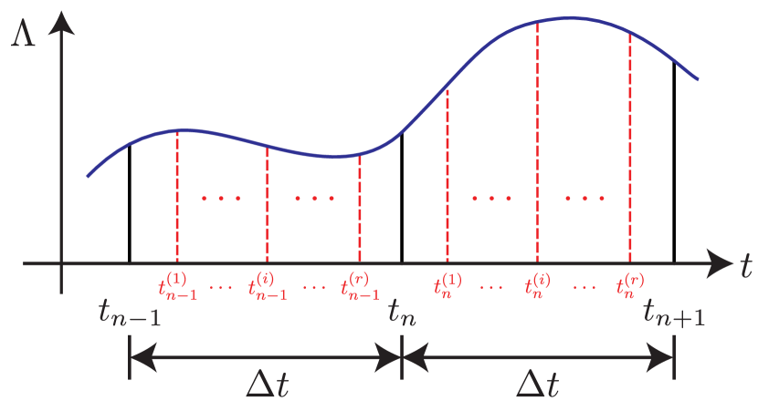
Figure 1.— The time discretization used for the Galerkin-Gauss-Lobatto (GGL) variational integrator. The action is approximated using the Gauss-Lobatto quadrature method, where for each interval $\Delta t$, the area under the nonconservative Lagrangian is approximated by the weighted sum of the Lagrangian, $\Lambda(q_{\pm},\dot{q}_{\pm},t)$, evaluated at each of the $(r+2)$ quadrature points. This quadrature rule (and the variational integrator) is accurate up to order $(2r+2)$. The generalized velocities $\dot{q}_{\pm}$ are approximated using the derivative of the $(r+1)$th-order interpolating function at each quadrature point.

We then have the approximation $\dot{q}_{n,\pm}(t)\simeq\dot{\phi}_{n,\pm}(t)$, which can be conveniently evaluated at the quadrature points using the derivative matrix (see e.g. Boyd, 2001, 2015),

$$D_{ij}=\begin{cases}\hfil-{(r+1)(r+2)}/({2\Delta t})&\qquad i=j=0\\ \hfil{(r+1)(r+2)}/({2\Delta t})&\qquad i=j=r+1\\ \hfil 0&\qquad i=j\neq 0,r+1\\ \hfil\displaystyle\frac{2P_{r+1}(x_{i})}{P_{r+1}(x_{j})(x_{i}-x_{j})\Delta t}&\qquad i\neq j\end{cases}$$ (5)

such that

$$\dot{\phi}_{n,\pm}(t_{n}^{(i)})=\sum_{j=0}^{r+1}D_{ij}\,q_{n,\pm}^{(j)}\equiv\dot{\phi}_{n,\pm}^{(i)}$$ (6)

where for notational compactness we define $t_{n}^{(0)}\equiv t_{n}$, $t_{n}^{(r+1)}\equiv t_{n+1}$, and $q_{n,\pm}^{(i)}\equiv q_{\pm}(t_{n}^{(i)})$.

Using Gauss-Lobatto quadrature, any integral functional $\int Fdt$ [for example $F\in\{\Lambda,L,K\}$] has a discrete-quadrature approximation on the time interval $[t_{n},t_{n+1}]$. This discrete functional $F_{d}^{n}$ is

$$F_{d}(q_{n,\pm},\{q_{n,\pm}^{(i)}\}_{i=1}^{r},q_{n+1,\pm},t_{n}) \equiv\sum_{i=0}^{r+1}w_{i}F(q_{n,\pm}^{(i)},\dot{\phi}_{n,\pm}^{(i)},t_{n}^{(i)})$$

$$\equiv F_{d}^{n},$$ (7)

where the Gauss-Lobatto quadrature weights $w_{i}$ are given by

$$w_{i}\equiv\frac{\Delta t}{(r+1)(r+2)[P_{r+1}(x_{i})]^{2}}.$$ (8)

Now we approximate the action over an interval $[t_{0},t_{N+1}]$,

$${\cal S}[t_{0},t_{N+1}] =\int_{t_{0}}^{t_{N+1}}\Lambda(q_{\pm},\dot{q}_{\pm},t)dt$$

$$={\cal S}_{d}[t_{0},t_{N+1}]+{\cal O}(\Delta t^{2r+3}),$$ (9)

where the discretized action is defined as

$${\cal S}_{d}[t_{0},t_{N+1}]\equiv\sum_{n=0}^{N}\Lambda_{d}(q_{n,\pm},\{q_{n,\pm}^{(i)}\}_{i=1}^{r},q_{n+1,\pm},t_{n}).$$ (10)

We refer to this discretization choice as the Galerkin-Gauss-Lobatto (GGL) method (Farr & Bertschinger, 2007).

The discrete action ${\cal S}_{d}[t_{0},t_{N+1}]$ from (10) can then be extremized over values $q_{n,-}$ and $q_{n,-}^{(i)}$, and the physical limit imposed, to generate the discretized equations of motion for each $n\in[1,N]$,

$$\left[\frac{\partial\Lambda_{d}^{n-1}}{\partial q_{n,-}}+\frac{\partial\Lambda_{d}^{n}}{\partial q_{n,-}}\right]_{\rm PL} =0,$$ (11a)

$$\left[\frac{\partial\Lambda_{d}^{n}}{\partial q_{n,-}^{(i)}}\right]_{\rm PL} =0,$$ (11b)

since from Figure 1, we see that each $q_{n,-}^{(i)}$ only contributes to a single $\Lambda_{d}^{n}$ in the discretized action (10), while each $q_{n,-}$ appears in both $\Lambda_{d}^{n-1}$ and $\Lambda_{d}^{n}$.

In terms of $L_{d}^{n}$ and $K_{d}^{n}$, the equations of motion are

$$\frac{\partial L_{d}^{n-1}}{\partial q_{n}}+\frac{\partial L_{d}^{n}}{\partial q_{n}}+\left[\frac{\partial K_{d}^{n-1}}{\partial q_{n,-}}+\frac{\partial K_{d}^{n}}{\partial q_{n,-}}\right]_{\rm PL} =0$$ (12a)

$$\frac{\partial L_{d}^{n}}{\partial q_{n}^{(i)}}+\left[\frac{\partial K_{d}^{n}}{\partial q_{n,-}^{(i)}}\right]_{\rm PL} =0.$$ (12b)

We now introduce the discrete momenta $\pi_{n}$, defining the nonconservative (slimplectic) GGL variational integrator map $(q_{n},\pi_{n})\rightarrow(q_{n+1},\pi_{n+1})$, by splitting the equation of motion (12a) into

$$\pi_{n} \equiv-\left[\frac{\partial\Lambda_{d}^{n}}{\partial q_{n,-}}\right]_{\rm PL} ={} -\frac{\partial L_{d}^{n}}{\partial q_{n}}-\left[\frac{\partial K_{d}^{n}}{\partial q_{n,-}}\right]_{\rm PL},$$ (13a)

$$\pi_{n+1} \equiv\left[\frac{\partial\Lambda_{d}^{n}}{\partial q_{n+1,-}}\right]_{\rm PL} ={} \frac{\partial L_{d}^{n}}{\partial q_{n+1}}+\left[\frac{\partial K_{d}^{n}}{\partial q_{n+1,-}}\right]_{\rm PL},$$ (13b)

$$0 =\left[\frac{\partial\Lambda_{d}^{n}}{\partial q^{(i)}_{n,-}}\right]_{\rm PL} ={} \frac{\partial L_{d}^{n}}{\partial q_{n}^{(i)}}+\left[\frac{\partial K_{d}^{n}}{\partial q_{n,-}^{(i)}}\right]_{\rm PL}.$$ (13c)

Given initial values of $(q_{n},\pi_{n})$, the values of $q_{n+1}$ are determined implicitly by (13a), while the values for the $q_{n}^{(i)}$ intermediate points are given implicitly by equation (13c) for $i\in\{1\ldots r\}$. The final momenta $\pi_{n+1}$ can then be determined explicitly from (13b).

Noether’s theorem for conservative actions can be shown to generalize to nonconservative systems where the corresponding Noether currents evolve in time due to a non-zero K (Galley, Tsang, & Stein, 2014). One can show that for continuous symmetries of the conservative action, which remain after discretization, discrete Noether currents will also evolve due to $K_{d}$. Thus, translational or rotational symmetries, for example, will generate discrete momenta that evolve according to $K_{d}$, up to round off and bias error (Brouwer, 1937; Rein & Spiegel, 2015). Additional error compared to the physical evolution is only due to the discretization of the action.

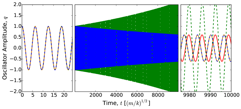
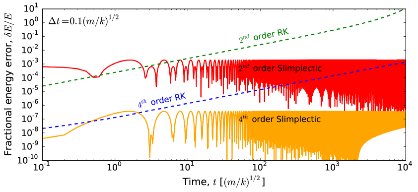
Figure 2.— Top: Numerical solutions for the damped harmonic oscillator, described by $L=m\dot{q}^{2}/2-kq^{2}/2$, $K=-\lambda\dot{q}_{+}q_{-}$, with $\lambda=10^{-4}(mk)^{1/2}$, and fixed time steps $\Delta t=0.1(m/k)^{1/2}$. Initial conditions were taken to be $q(0)=1$ and $\dot{q}(0)=0$. The $2$nd order RK solution, shown in green, is unstable for these parameters and diverges significantly. The $4$th-order RK solution (blue-dashed) cannot be readily distinguished from the $4$th-order slimplectic solution (solid-orange) in this plot. The $2$nd-order slimplectic solution, (solid-red), gives nearly the correct amplitude after $\sim 10^{5}$ time steps, as the energy evolution is accurately followed, though a phase shift is evident. Bottom: The fractional energy error relative to the energy given by the analytic solution at each time. We see that while initially the RK and slimplectic energy errors are comparable at each order, the RK energy errors grow roughly linearly with time, while the slimplectic energy error remains bounded.

The GGL discretization does not preserve the time-shift symmetry preventing energy evolution from being precisely tracked. However, the fractional energy error tends to be oscillatory and bounded by a resolution and order-dependent constant. We will defer more detailed discussion of Noether current evolution to a longer followup paper in the interests of space.

The resulting slimplectic maps are accurate up to order $2r+2$. For $r=0$, where no intermediate steps are used, the quadrature method is the trapezoid rule, and the variational integrator is 2nd-order and equivalent to the Störmer-Verlet “leap-frog” integrator (Wendlandt & Marsden, 1997).

It is well known that 2nd-order “leap-frog” integrators can be used for dissipative systems, by inserting a dissipative “kick” force into the “kick-drift-kick” ansatz, resulting in good energy and momentum evolution properties. Our approach explains why this simple modification works in the 2nd-order system, as it is equivalent to the lowest order slimplectic GGL method (see also Lew et al., 2004, for a similar Lagrange-d’Alembert approach). The slimplectic method allows this to be generalized to higher orders and general nonconservative systems.

4. Code and Examples

We have developed a simple python code, slimplectic, that is publicly available and generates the fixed-time-step slimplectic GGL integrators described above, for use in characterizing the numerical technique. The code generates slimplectic solvers of arbitrary order $(2r+2)$ given sympy (SymPy Dev Team, 2014) expressions for $L(q,\dot{q},t)$ and $K(q_{\pm},\dot{q}_{\pm},t)$. This demonstration code is designed to work for arbitrary $L$ and $K$, and thus has not been optimized as would be appropriate for specific problems. In particular, the equations of motion (13) are solved with standard root-finders, rather than a problem-specific iteration method, to be more generally applicable.

As a basic example in Figure 2 we compare Runge-Kutta (RK) and slimplectic integration of a simple damped harmonic oscillator, for both 2nd and 4th-order methods. Below we also present two basic astrophysical examples of non-conservative interactions. All examples are available as ipython notebooks in our public repository.⁵

4.1. Poynting-Robertson Drag

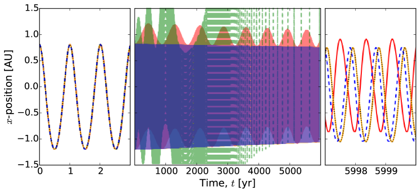
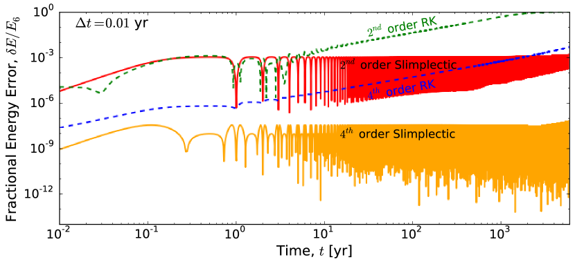
Figure 3.— Top: Evolution of the Cartesian x-coordinate for orbital motion of a particle experiencing Poynting-Robertson drag due to radiation from a solar-type star, with particle density $\rho=2$ g cm^-3 and particle size $d=5\times 10^{-2}$ cm. The particle has initial semi-major axis of 1AU, and initial eccentricity of $0.2$. With a fixed-time-step of $\Delta t=0.01$ yr, the 2nd-order RK integrator (green-dashed) is unstable, while the 2nd-order slimplectic integrator (red) behaves much more accurately, despite significant (numerical) precession over a $\sim$1000 year timescale. The 4th-order integrators (RK, blue-dashed; slimplectic, orange) have similar long-term amplitude evolution without visible numerical precession. The phase errors (not shown) of the RK integrators grow $\propto t^{2}$, while the slimplectic integrators have phase error $\propto t$ (see Preto & Tremaine, 1999). Bottom: Fractional energy error (compared to a 6th-order slimplectic integration) for the system described above. The RK errors grow roughly linearly in time, while the slimplectic errors are bounded. There is a slight turn-up in the 4th-order slimplectic error envelope, most likely due to the build up of round-off, bias, or action-discretization error.

We first examine the orbital motion of a dust particle experiencing Poynting-Robertson drag (Burns et al., 1979) due to radiation from a solar type star, starting with a semi-major axis of 1AU in an eccentric ($e=0.2$) orbit. The Lagrangian for this system is

$$L=\frac{1}{2}m\dot{\mathbf{q}}^{2}+(1-\beta)\frac{GM_{\odot}m}{|{\mathbf{q}}|},$$ (14)

where $m$ is the dust particle’s mass, and ${\mathbf{q}}$ its position. The dimensionless factor

$$\beta\equiv\frac{3L_{\odot}}{8\pi c\rho\,GM_{\odot}d}\simeq 0.058\left(\frac{\rho}{2\,{\rm g}\,{\rm cm}^{-3}}\right)^{-1}\left(\frac{d}{10^{-3}{\rm cm}}\right)^{-1},$$ (15)

is the ratio between forces due to radiation pressure and gravity, where $L_{\odot}$ and $M_{\odot}$ are the solar luminosity and mass, $\rho$ and $d$ are the density and size of the dust grain. The nonconservative potential which generates the correct Poynting-Robertson drag force is (for $|\dot{\mathbf{q}}|\ll c$) found as the virtual work from the known force,

$$K=-\frac{\beta GM_{\odot}m}{c\,{\mathbf{q}}_{+}^{2}}\left[\dot{{\mathbf{q}}}_{+}\cdot{\mathbf{q}}_{-}+\frac{1}{{\mathbf{q}}_{+}^{2}}(\dot{{\mathbf{q}}}_{+}\cdot{\mathbf{q}}_{+})({\mathbf{q}}_{+}\cdot{\mathbf{q}}_{-})\right].$$ (16)

Methods to determine or derive $K$ are discussed in (Galley et al., 2014). The first term in square brackets above gives the usual drag term, while the second term is due to the Doppler shift caused by radial motion.

The system was integrated for $6000$ years using 2nd and 4th-order RK (green and blue dashed) and slimplectic (red and orange solid) methods with time-steps of $\Delta t=0.01$ yr. The results and discussion are shown in Figure 3.

4.2. Gravitational Radiation Reaction

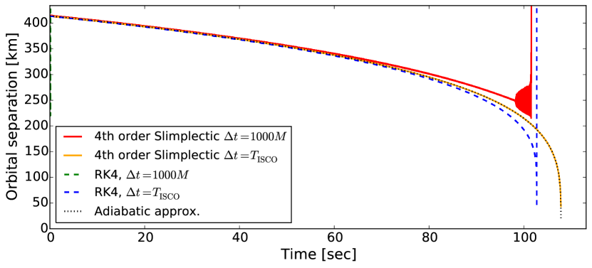
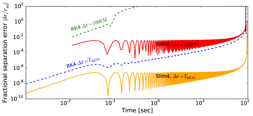
Figure 4.— Top: PN radiation reaction, including only the 2.5PN dissipative terms through $K$. Each of the methods (RK and slimplectic GGL) are 4th order with fixed timesteps of $\Delta t=1000M$ and $\Delta t=T_{\rm ISCO}$. The integration methods blow up when the orbital time-scale is comparable to the time step, though the slimplectic method performs significantly better than the RK method for the same time steps; for the $1000M$ time-step the RK method is immediately unstable.
Bottom: Relative error in the orbital radius compared to the analytic adiabatic-approximation solution.

We also consider two $1.4M_{\odot}$ neutron stars inspiraling from gravitational wave emission. This example demonstrates (fixed-time-step) integrators for systems where the orbital dynamics can change quickly due to nonconservative effects. In the post-Newtonian (PN) approximation, leading-order conservative dynamics for the orbital separation, ${\mathbf{q}}$, are described by Newtonian gravity

$$L=\frac{1}{2}\mu\dot{\mathbf{q}}^{2}+\frac{\mu M}{|{\mathbf{q}}|},$$ (17)

where $M=m_{1}+m_{2}=2.8M_{\odot}$ is the total mass, $\mu=m_{1}m_{2}/M=0.7M_{\odot}$ is the reduced mass, and $G=c=1$.

Dissipative effects from radiation reaction first appear at PN order $(|\dot{\mathbf{q}}|/c)^{5}$ (or 2.5PN) and are described by $K$, which has been calculated in Galley & Leibovich (2012); Galley & Tiglio (2009). After order-reduction,

$$K={} \frac{16}{5}\nu^{2}M^{4}\frac{(\dot{\mathbf{q}}_{+}\cdot{\mathbf{q}}_{-})}{|{\mathbf{q}}_{+}|^{4}}-\frac{48}{5}\nu^{2}M^{3}\frac{|\dot{\mathbf{q}}_{+}|^{2}(\dot{\mathbf{q}}_{+}\cdot{\mathbf{q}}_{-})}{|{\mathbf{q}}_{+}|^{3}}$$

$${}+24\nu^{2}M^{3}\frac{(\dot{\mathbf{q}}_{+}\cdot{\mathbf{q}}_{+})^{2}(\dot{\mathbf{q}}_{+}\cdot{\mathbf{q}}_{-})}{|{\mathbf{q}}_{+}|^{5}}$$

$${}+\frac{16}{15}\nu^{2}M^{4}\frac{(\dot{\mathbf{q}}_{+}\cdot{\mathbf{q}}_{+})({\mathbf{q}}_{+}\cdot{\mathbf{q}}_{-})}{|{\mathbf{q}}_{+}|^{6}}$$

$${}+\frac{144}{5}\nu^{2}M^{3}\frac{|\dot{\mathbf{q}}_{+}|^{2}(\dot{\mathbf{q}}_{+}\cdot{\mathbf{q}}_{+})({\mathbf{q}}_{+}\cdot{\mathbf{q}}_{-})}{|{\mathbf{q}}_{+}|^{5}}$$

$${}-40\nu^{2}M^{3}\frac{(\dot{\mathbf{q}}_{+}\cdot{\mathbf{q}}_{+})^{3}({\mathbf{q}}_{+}\cdot{\mathbf{q}}_{-})}{|{\mathbf{q}}_{+}|^{7}}\,,$$ (18)

where $\nu=\mu/M=1/4$. A physically consistent simulation should go to the same PN order in $L$ and $K$. Here, instead, we use the leading order in each as a toy model to focus on the numerical method.

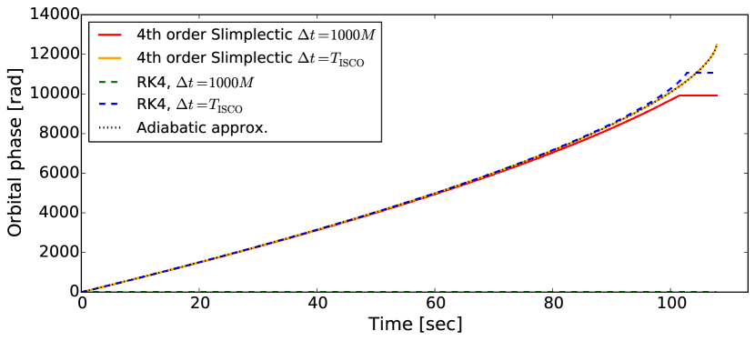
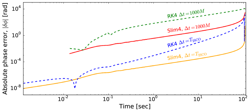
Figure 5.— Top: The phase evolution of the integrators for the PN radiation reaction depicted in Figure 4.
Bottom: Absolute orbital-phase errors. In this example, both slimplectic integrators (phase error $\propto t$), track the orbital phase much better than the equivalent RK integrators (phase error $\propto t^{2}$).

In Figures 4 and 5 we examine the 4th-order RK and slimplectic integrators for different choices of time steps, $\Delta t=1000M$ and $\Delta t=T_{\rm ISCO}\simeq 92M$, the orbital period at the innermost stable circular orbit. The initial orbital separation is $r_{0}=100M\approx 414$km and corresponds to an orbital frequency of $\approx 11.5$Hz. We compare our numerical results to analytic solutions to our toy PN equations in the adiabatic regime,

$$r_{\rm ad}(t)\!=\!\left(r_{0}-\frac{256}{5}\nu M^{3}t\right)^{\!1/4}{\hskip-7.22743pt},~{}\phi_{\rm ad}(t)\!=\!\frac{r_{0}^{5/2}-r_{\rm ad}^{5/2}(t)}{32\nu M^{5/2}}\,,$$

where the orbital period is assumed to be much smaller than the radiation reaction time scale for the inspiral (Blanchet, 2014).

All integrators begin to fail when the orbital period becomes roughly comparable to the time-step, although the slimplectic integrators can get significantly closer to this limit than the RK method (the RK integrator with time-step $\Delta t=1000M$ immediately becomes unstable). In our followup paper, we will demonstrate an adaptive time-stepping scheme that will allow efficient slimplectic integrations that also precisely evolve the energy.

5. Discussion

We have developed a new method of numerical integration that combines the nonconservative action principle of Galley (2013); Galley et al. (2014) with the variational-integrator approach of Marsden & West (2001). These “slimplectic” integrators allow nonconservative effects to be included in the numerical evolution, while still possessing the major benefits of normally conservative symplectic integrators, particularly the accurate long-term evolution of momenta and energy.

The discrete equations of motion are found by varying a discretized nonconservative action and implicitly define the slimplectic mapping $(q_{n},\pi_{n})\rightarrow(q_{n+1},\pi_{n+1})$. Different choices of discretization generate different variational integrators. Here we have focused on implementing the Galerkin-Gauss-Lobatto (GGL) discretization, and demonstrating its long-term accuracy using the damped harmonic oscillator, Poynting-Robertson drag on a small particle, and a gravitational radiation-reaction toy problem. Our results also explain why the modification of the 2nd-order “kick-drift-kick” ansatz to include dissipative forces performs so accurately, as this is equivalent to the lowest order version of the slimplectic GGL method.

We have developed a demonstration python code, slimplectic,⁵ which generates slimplectic integrators for arbitrary Lagrangians and nonconservative potentials. Readers are encouraged to test different physical systems of interest using this publicly available code, but to separately implement problem specific optimizations, particularly when solving the implicit equations of motion.

Acknowledgments — We thank A. Cumming, A. Archibald, D. Tamayo, D.P. Hamilton, M.C. Miller, and the referee, W. Farr, for useful discussion. D.T. was supported by the Lorne Trottier Chair in Astrophysics and Cosmology and CRAQ. C.R.G. was supported in part by NSF grants CAREER PHY-0956189 and PHY-1404569 at Caltech. L.C.S. was supported by NASA through Einstein Postdoctoral Fellowship Award Number PF2-130101.

References

- Blanchet (2014) Blanchet, L. 2014, Living Reviews in Relativity, 17, 2
- Boyd (2001) Boyd, J. 2001, Chebyshev and Fourier Spectral Methods: Second Revised Edition, Dover Books on Mathematics (Dover Publications)
- Boyd (2015) —. 2015, Errata in second edition of Chebyshev and Fourier Spectral Methods, http://www-personal.umich.edu/~jpboyd/errata_dover2dedition.pdf, [Online; accessed 02-Apr-2015]
- Brouwer (1937) Brouwer, D. 1937, AJ, 46, 149
- Brown (2006) Brown, J. D. 2006, Phys. Rev. D, 73, 024001
- Burns et al. (1979) Burns, J. A., Lamy, P. L., & Soter, S. 1979, Icarus, 40, 1
- Cordeiro et al. (1996) Cordeiro, R. R., Gomes, R. S., & Vieira Martins, R. 1996, Celestial Mechanics and Dynamical Astronomy, 65, 407
- Farr (2009) Farr, W. M. 2009, Celestial Mechanics and Dynamical Astronomy, 103, 105
- Farr & Bertschinger (2007) Farr, W. M., & Bertschinger, E. 2007, ApJ, 663, 1420
- Galley (2013) Galley, C. R. 2013, Physical Review Letters, 110, 174301
- Galley & Leibovich (2012) Galley, C. R., & Leibovich, A. K. 2012, Phys. Rev. D, 86, 044029
- Galley & Tiglio (2009) Galley, C. R., & Tiglio, M. 2009, Phys. Rev. D, 79, 124027
- Galley et al. (2014) Galley, C. R., Tsang, D., & Stein, L. C. 2014, ArXiv e-prints, arXiv:1412.3082
- Ge & Marsden (1988) Ge, Z., & Marsden, J. E. 1988, Phys. Lett. A, 133, 134
- Gladman et al. (1991) Gladman, B., Duncan, M., & Candy, J. 1991, Celestial Mechanics and Dynamical Astronomy, 52, 221
- Hamilton et al. (1999) Hamilton, D. P., Rauch, K., & Burns, J. A. 1999, in Bulletin of the American Astronomical Society, Vol. 31, AAS/Division of Dynamical Astronomy Meeting #31, 1223
- Kane et al. (1999) Kane, C., Marsden, J. E., & Ortiz, M. 1999, Journal of mathematical physics, 40, 3353
- Levison & Duncan (1994) Levison, H. F., & Duncan, M. J. 1994, Icarus, 108, 18
- Lew et al. (2003) Lew, A., Marsden, J. E., Ortiz, M., & West, M. 2003, Archive for Rational Mechanics and Analysis, 167, 85
- Lew et al. (2004) Lew, A., Marsden, J. E., Ortiz, M., & West, M. 2004, International Journal for Numerical Methods in Engineering, 60, 153
- Malhotra (1994) Malhotra, R. 1994, Celestial Mechanics and Dynamical Astronomy, 60, 373
- Marsden & West (2001) Marsden, J. E., & West, M. 2001, Acta Numerica 2001, 10, 357
- Mikkola (1997) Mikkola, S. 1997, Celestial Mechanics and Dynamical Astronomy, 68, 249
- Preto & Tremaine (1999) Preto, M., & Tremaine, S. 1999, AJ, 118, 2532
- Rein & Spiegel (2015) Rein, H., & Spiegel, D. S. 2015, MNRAS, 446, 1424
- Rein & Tamayo (2015) Rein, H., & Tamayo, D. 2015, ArXiv e-prints, arXiv:1506.01084
- SymPy Dev Team (2014) SymPy Dev Team. 2014, SymPy: Python library for symbolic mathematics
- Wendlandt & Marsden (1997) Wendlandt, J. M., & Marsden, J. E. 1997, Physica D Nonlinear Phenomena, 106, 223
- Wisdom & Holman (1991) Wisdom, J., & Holman, M. 1991, AJ, 102, 1528
- Zhang & Hamilton (2007) Zhang, K., & Hamilton, D. P. 2007, Icarus, 188, 386