Calibration of Lévy Processes using Optimal Control of Kolmogorov Equations with Periodic Boundary Conditions

Abstract

We present an optimal control approach to the problem of model calibration for Lévy processes based on a non parametric estimation procedure. The calibration problem is of considerable interest in mathematical finance and beyond. Calibration of Lévy processes is particularly challenging as the jump distribution is given by an arbitrary Lévy measure, which form a infinite dimensional space. In this work, we follow an approach which is related to the maximum likelihood theory of sieves [21]. The sampling of the Lévy process is modelled as independent observations of the stochastic process at some terminal time $T$. We use a generic spline discretization of the Lévy jump measure and select an adequate size of the spline basis using the Akaike Information Criterion (AIC) [13].

The numerical solution of the Lévy calibration problem requires efficient optimization of the log likelihood functional in high dimensional parameter spaces. We provide this by the optimal control of Kolmogorov’s forward equation for the probability density function (Fokker-Planck equation). The first order optimality conditions are derived based on the Lagrange multiplier technique in a functional space. The resulting Partial Integral-Differential Equations (PIDE) are discretized, numerically solved and controlled using scheme a composed of Chang-Cooper, BDF2 and direct quadrature methods. For the numerical solver of the Kolmogorov’s forward equation we prove conditions for non-negativity and stability in the $L^{1}$ norm of the discrete solution. To set boundary conditions, we argue that any Lévy process on the real line can be projected to a torus, where it again is a Lévy process. If the torus is sufficiently large, the loss of information is negligible.

MSC (2010): 93E10 (primary) 49K20, 60G51, 62G05 (secondary)

Key words: Optimal control of PIDE, Kolmogorov equations, Fokker-Planck equation, Lévy processes, non-parametric maximum likelihood method, Akaike information criterion, financial data.

1 Introduction

Lévy processes play a large rôle in contemporary mathematical finance [15], but also in many areas of physics, see e.g. [2, 26]. A real valued Lévy process is a stochastic process $Y(t)$ that has increments $Y(t)-Y(s)$, $t\geq s$, that are independent of the past. The increments are also stationary in the sense that the probability distribution of the increment only depends on the time difference $t-s$. Furthermore, $Y(0)=0$ and a stochastic continuity condition for $t=0$ holds, see e.g. [2]. Under the given conditions, the characteristic function of $Y(t)$ is given by the Lévy Khinchine representation

$$\mathbb{E}\left[e^{iY(t)k}\right]=e^{t\psi(k)}$$ (1)

$\mathbb{E}[\cdot]$ stands for the expected value. $\psi(k)$ is a conditionally positive definite function [8] that has the following representation in terms of the canonical triplet $(b,\sigma^{2},\nu)$:

$$\psi(k)=ibk-\frac{\sigma^{2}}{2}k^{2}+\int_{\mathbb{R}\setminus\{0\}}\left(e^{isk}-1-isk1_{\{|s|\leq 1\}}(s)\right)d\nu(s).$$ (2)

$b,\sigma^{2}\in\mathbb{R}$ are constants, $\sigma^{2}\geq 0$, and the Lévy measure $\nu$ is a positive measure on $\mathbb{R}\setminus\{0\}$ such that

$$\int_{\mathbb{R}\setminus\{0\}}\min(1,s^{2})d\nu(s)<\infty.$$ (3)

In Eq. (2) $1_{\{|s|\leq 1\}}(s)$ is the characteristic function of the set $\{|s|\leq 1\}$ which takes the value $1$ on this set and $0$ otherwise.

The calibration problem for Lévy processes consists of the estimation of the canonical triplet $(b,\sigma^{2},\nu)$ given the observation $Y(t_{j})$ of the process’ trajectory $Y(t)$ at some prescribed times $t_{j}$, $j=1,\ldots,L$. For instance, $Y(t)$ could be the process of log-Returns of some asset and $t_{j}$ could be the closing time of the $j$-th trading day (’historic low frequency data’). As the $j$-th increment of the process $Y_{j}=Y(t_{j})-Y(t_{j-1})$ has the same distribution as $Y(T)$, if $T=t_{j}-t_{j-1}$, from a statistical point of view this is equivalent to the $L$-fold independent observation of the terminal values $Y(T)$ at time $T$.

$Y(t)$ can also be understood as the solution to the Stochastic Differential Equation (SDE) of jump-diffusion type

$$dY(t)=bdt+\sigma dB(t)+\int_{\{|y|\leq 1\}}y\tilde{N}(dt,dy)+\int_{\mathbb{R}\setminus\{|y|>1\}}yN(dt,dy),~{}~{}Y(0)=0.$$ (4)

Here $B(t)$ is a standard Brownian motion and $N((t,t+\Delta t],A)\sim{\rm Po}(\nu(A)\Delta t)$ is the random counting measure of jumps of height in the set $A\subseteq\mathbb{R}$ in the time interval $(t,t+\Delta t]$. ${\rm Po}(\lambda)$ stands for the Poisson distribution with intensity $\lambda$ and $\tilde{N}((t,t+\Delta t],A)=N((t,t+\Delta t],A)-\nu(A)\Delta t$ is the compensated or Martingale jump measure for small jumps, where we require $A\subset\mathbb{R}\setminus\{|x|\leq\varepsilon\}$ for some $\varepsilon>0$, see [2] for further details.

The calibration problem for Lévy processes, respectively the solution of (4), unfortunately is ill posed: The collection of all Lévy measures $\nu$ is infinite dimensional, while only $L$ observations are available. Direct application of the maximum likelihood principle in this situation leads to severe over-fitting issues [21]. In many applications, one chooses families of Lévy measures $\nu(\bar{\alpha})$ that depend only on a finite dimensional parameter vector $\bar{\alpha}$, see e.g. [24]. Furthermore, one often restricts to such parametrizations, where the density $f(x,T,\bar{\alpha})$ of the probability distribution of $Y(t)$ can be calculated explicitly or at low numerical cost. One then assumes that the true distribution of $Y(t)$ is inside the prescribed set and uses the maximum likelihood approach for calibration [19]. This assumption might however not be justified and give rise to modelling errors.

As a non-parametric alternative, one can use generic parametrizations for the density of the Lévy measure $\nu$ that can be refined depending on the amount of data available. This gives rise to a hierarchy – or sieve [21] – of maximum likelihood problems with a finite number of parameters. If a suitable finite parametrization has been chosen, it remains to solve the maximum likelihood estimate at a given level of parametrization. One also has to determine this level based on the quality and also stability of the fits obtained. The resulting densities can no longer be calculated analytically. Also, solution of the maximum likelihood problem gives rise to high dimensional optimization problems.

The maximum likelihood method requires a parametric representation of the probability density functions (PDF). The PDF can however be obtained as a solution to the Kolmogorov forward equation (Fokker Planck equation). The parameters $\bar{\alpha}$ then enter in this equation via coefficients in the generator of the semigroup [2]. If the Lévy measure $\nu$ is not zero, the generator of both these equations does not only contain a 2nd order partial differential operator, but also an integral operator of convolution type. This places the model calibration problem in the framework of optimal control problems with partial integral differential equations (PIDE) constraints.

Indeed, we know that the Kolmogorov forward equation is representative of a stochastic process described in terms of SDEs such as that one of Eq. (4), where the set of parametrization for the approximation of the PDF, would correspond to a set of controls of the stochastic dynamic equation, so that, jointly to the maximum likelihood problem, it corresponds to a stochastic optimal control problem. The classical way to deal with the optimal control of stochastic process is by the Dynamic Programming principle and the related Hamilton-Jacobi-Bellman equation for stochastic processes [9]. However, this problem has been recently framed as a constrained PDE optimization problem, where the PDE is the Fokker-Planck, i.e. Kolmogorov forward, equation [3, 4, 5]. Following this framework, the solution of the maximum likelihood problem, i.e. the stochastic optimization, is found by solving the first order optimality conditions in a functional space, that is the optimality system consisting of two PIDEs, named forward and backward (or adjoint) equations, plus an optimality condition.

This optimality system can be numerically solved by a gradient-based iterative algorithm as follows. The Kolmogorov forward equation has a set of control parameters in order to maximize the log-Likelihood functional for its terminal value. These controls involve the Kolmogorov backward equation (adjoint equation) with suitable terminal condition, corresponding to the log-likelihood functional. Hence, given an initial approximation of the unknown parametrization, first solve the forward equation, then set up the terminal condition and solve the adjoint one. With both the forward and adjoint solutions, by using the optimality condition equation the gradient is computed. Then with a descending gradient technique, such as a non linear conjugate gradient method, found a better approximation of the control parameters and repeat until the satisfying accuracy for the parametrization is found.

Since this maximum likelihood problem could have an high dimensional space ad a huge number $L$ of observations, a fast, stable and enough accurate numerical solver for the PIDE is required. In our case the Kolmogorov forward equation is a PIDE of parabolic differential operator type. Such kind of PIDEs are, e.g., investigated in the option pricing models as a generalization of the Black-Scholes equation. The first difficulty to numerically solve this equation is the integral. In fact, in the case of using a fully implicit method, it would lead to solve a dense system of equation, for this reason implicit-explicit (IMEX) or operator splitting methods can be applied to bypass this problem (see [18, 10, 16]). The solution of the Kolmogorov forward equation is a probability density function that is non negative with constant integral over the domain. Such properties must be owned from the discrete solution too. The Chang-Cooper (CC) is a non-negative and conservative numerical method that has been used to solve the classical Fokker-Planck equation [14, 4, 11]. Here, we use a numerical method that can be classified as IMEX, since we use the CC method with an implicit time difference scheme for the differential operators of our PIDE, and evaluate the integral operator at the previous time step solution, i.e. in an explicit way. We prove for the resulting numerical solver: conservativeness, non-negativity and stability in the $L^{1}$-norm. The numerical solver for the adjoint equation is obtained directly from the solver for the forward equation by using the “discretize then optimize” approach to the optimization problem.

Finally, we quote, that for related work with vanishing Lévy measure see e.g. [4, 12], and for estimation procedures based on non parametric approximations of the empirical characteristic function see e.g. [7]. An approach based on the method of moments and asymptotic expansions of Lévy densities can be found in [22].

The article is organised as follows: In the following Section 2 we describe the hierarchy, of estimation problems. We shall show that the estimation problems that can actually be solved numerically can come arbitrarily close, at increasing computational cost, to the fully general Lévy estimation problem. We also show that the use of periodic boundary conditions in the Kolmogorov equations can be understood in terms of mapping the original Lévy process on the real line to a derived Lévy process on the torus.

In Section 3, we set up the maximum likelihood estimation problem for a given parametrization and derive Kolmogorov’s forward (Fokker-Planck) equation and its adjoint (Kolmogorov backward) equation with terminal conditions set by the log-Likelihood objective functional. This maximum likelihood estimation problem is solved in the framework of the Fokker-Planck optimal control of stochastic processes, as a constrained PDE optimal control problem.

In Section 4 the discretization for Kolmogorov’s equations and the optimal control scheme is derived following a Chang-Cooper and IMEX approach. In particular we prove the structural properties of the numerical solution, i.e. conservativeness, non-negativity and stability.

Section 5 gives numerical tests for the consistency of the proposed procedure based on simulated data. We propose to use Akaike’s information criterion (AIC) [13] to choose an adequate parametrization from the hierarchy of spline parametrizations for density of the Lévy measure. Three different tests are performed: We first fit data that are simulated from a given distribution within our hierarchy of Lévy distributions. The fits obtained are shown to be of very good quality and AIC-selection criterion reproduces almost the original parametrization. As a second test we fit simulated data from a bi-directional Gamma process, i.e. the difference of two independent Gamma processes [2], which is not inside one of the parametrizations of degree $N_{\Theta}$, but can be approximated by those. The bi-directional Gamma process is augmented by a small diffusive component and projected to the torus. The AIC selection criterion and the fitting results again reproduce the final distribution of this process rather adequately. As a final test, we select financial data from the German stock exchange DAX in a period between April 1998 and March 2002 and consider daily log-returns over 1000 trading days. This period represents a rather stable period for the DAX with an almost constant level of the volatility. After projection, the AIC based method selects a six-parameter spline approximation of the Lévy measure density. The resulting fits again give a decent reproduction of the empirical distribution.

Our conclusions and an outlook are given in the final Section 6.

2 A Hierarchy of Parametrizations for Maximum Likelihood Estimation of Lévy Data

The estimation problem for the Lévy measure $\nu$ is plagued by several issues. Here we take a step by step approach towards the derivation of a hierarchy of estimation problems that approximate the original one.

Let $f(x|\bar{\alpha})=f(x|\bar{\alpha},N_{\Theta})$, $\bar{\alpha}\in\mathbb{R}^{N_{\Theta}}$, be a family of probability density functions with variable dimension $N_{\Theta}$ of the parameter set $\bar{\alpha}$, and let $f(x)$ be the (unknown) probability density of $Y_{t}$.

For $N_{\Theta}$ fixed, we apply the Maximum Likelihood method to select an estimated value $\hat{\alpha}$ based on increasing sample size. It is known from the general theory of Maximum Likelihood [19] that the estimated $\hat{\alpha}$ converges almost surely to the true value $\bar{\alpha}$, provided $f(x)=f(x|\bar{\alpha},N_{\Theta})$ holds.

This leaves the question open, which parametrization – or which value for $N_{\Theta}$– one should choose. We solve this problem by maximizing the Akaike Information Criterion (AIC). Maximizing the AIC corresponds to minimizing (asymptotically) the expected Kulback-Leibler distance, or relative entropy, between the true distribution $f(x)$ and its parametric estimate $f(x|\bar{\alpha},N_{\Theta})$. See [13][Chapter 6] for a detailed derivation.

Let us now define the parametrizations with $N_{\Theta}$ parameters. We intend to show that, for sufficiently large $N_{\theta}$, we can approximate the original Lévy distribution to an arbitrary precision. This requires several steps of approximation:

Truncating small and large jumps.

The total mass of the Lévy measure, $\lambda=\nu(\mathbb{R}\setminus\{0\})$, can be infinite. This quantity defines the average number of jumps per unit time of the associated Lévy process [2]. The easiest way to deal with this is to truncate small jumps by setting $\nu_{\varepsilon}=1_{\{|s|>\varepsilon\}}\nu$ which is a finite measure by equation (3). Using (3) and dominated convergence, one can moreover prove that $\psi_{\varepsilon}(k)\to\psi(k)$ for $k\in\mathbb{R}$ as $\varepsilon\searrow 0$. Here $\psi_{\varepsilon}(k)$ is given by (2) with $\nu$ replaced by $\nu_{\varepsilon}$. By the continuity theorem of Paul Lévy, see e.g. [6, Theorem 23.8], this then implies (weak) convergence in law of the respective probability distributions.

At the same time, a finite Lévy measure $\nu$ permits one to re-parametrize $\psi(k)$ of Eq. (2) via

$$\psi(k)=ibk-\frac{\sigma^{2}}{2}k^{2}+\int_{\mathbb{R}\setminus\{0\}}\left(e^{isk}-1\right)d\nu(s)$$ (5)

with $b\to b-\int_{\mathbb{R}\setminus\{0\}}s1_{\{|s|\leq 1\}}(s)d\nu(s)$. In the following we assume $\nu$ to be finite and use parametrization (5). The last term in (5) now has the structure of a compound Poisson distribution, i.e. $Y(t)$ can be represented as $Z(t)+\sum_{j=1}^{N(t)}U_{j}$ where $Z\sim\mathcal{N}(bt,\sigma^{2}t)$ is normally distributed, $N(t)\sim{\rm Po}(\lambda t)$ is Poisson distributed with intensity $\lambda t$ and $U_{j}$ are i.i.d. random variables with distribution given by the normalized Lévy measure, $U_{j}\sim\lambda^{-1}\nu$. Also $Z(t),N(t)$ and $U_{j}$ are all stochastically independent.

With a similar argument, we can cut off large jumps by replacing $\nu$ with $1_{\{|s|\leq\varepsilon^{-1}\}}\nu$. Also in this case, in the limit $\varepsilon\searrow 0$, the truncated Lévy distributions converge in law to the non truncated one. In the following we thus assume that the support of $\nu$ is contained in some finite interval $[\Omega_{a},\Omega_{b}]$. The appropriate size of this region can be estimated e.g. by the Chebyshev’s inequality using empirical mean and variance from the data.

Regularizing the Lévy measure.

Given a non negative, continuously differentiable function $\chi$ with compact support such that $\int_{\mathbb{R}}\chi(x)dx=1$, and setting $\chi_{\varepsilon}(x)=\frac{1}{\varepsilon}\chi(\frac{x}{\varepsilon})$, we define $\varrho_{\varepsilon}(s)=\chi_{\varepsilon}*\nu(s)=\int_{\mathbb{R}\setminus\{0\}}\chi_{\varepsilon}(s-\xi)d\nu(\xi)$. We consider the regularised measures $d\nu_{\varepsilon}(s)=\varrho_{\varepsilon}(s)ds$. Inserting this measure in (5), using Fubini’s theorem and dominated convergence, one easily shows that $\psi_{\varepsilon}(k)\to\psi(k)$. This again implies convergence of the related probability distributions in law.

Spline approximation of the densities.

Let thus $d\nu(s)=\varrho(s)ds$ with $\rho(s)$ non negative, continuously differentiable and with compact support. Let $\theta_{j}$, $j=1,\ldots,n+1$, be a collection of uniform grid points in $\mathbb{R}$ such that the support of $\varrho(x)$ is covered and $\theta_{j}-\theta_{j-1}=\Delta$. Define $\varrho_{\Delta}(s)$ by the linear interpolation between points $(\theta_{j},\varrho(\theta_{j}))$. Again, one easily sees that $\varrho_{\Delta}(s)$ converges to $\varrho(s)$ as $\Delta\searrow 0$. Also, for small $\Delta$, the functions $\varrho_{\Delta}(s)$ have support in a fixed compact interval and are uniformly bounded by the maximum value of $\varrho(s)$. If we insert measures $d\nu_{\Delta}(s)=\varrho_{\Delta}(s)d\nu(s)$ into (5), this expression converges to the related one with $d\nu(s)=\varrho(s)ds$. This suffices to prove that an approximation of the probability distributions (in law) is feasible with 1st order spline densities.

Fixing drift and diffusion terms.

One might or might not like to include the drift and diffusion term determined by $b$ and $\sigma^{2}$ into the estimation problem. Although, in general, these quantities have to be estimated, here we keep a small fixed value for $\sigma^{2}$ for reasons of numerical stability of the Kolmogorov equations. As long as this value underestimates the true diffusion, this corresponds to a splitting of the Lévy process $Y(t)=Z(t)+L(t)$ into stochastically independent components where $Z(t)$ is determined by the purely Gaussian Lévy triplet $(b,\sigma^{2},0)$. $L(t)$ will be a Lévy process that contains drift, the excess diffusion and jumps. However, the distribution of $L(t)$ at time $T$ can be approximated in the sense of convergence in law by compound Poisson distributions without drift and Lévy terms. The explicit construction can e.g. be found in [8]. We can thus approximate our estimation problem to arbitrary accuracy with a problem where drift and diffusion take fixed values. We also note that a non vanishing diffusion implies the existence of a probability density function $f(x,t)$ for the distribution of $Y(t)$.

Periodic boundary conditions from the projection to a torus.

Another problem with the Kolmogorov forward equation is the issue of boundary conditions. We have already shown that we can approximate the estimation problem by one where the Lévy measure $\nu$ has support inside a large interval $[\Omega_{a},\Omega_{b}]$. Let $\Omega$ be the torus $[\Omega_{a},\Omega_{b}]$ with the end points of the interval identified. Let $K=\Omega_{b}-\Omega_{a}$, then define the operator $+_{K}$ as $x+_{K}y:=(x+y)\mod(K)$ a group operation on $\Omega$, with $(\cdot)\mod(\cdot)$ the modulus operation. Let furthermore

$$\phi:(\mathbb{R},+)\to(\Omega,+_{K})$$ (6)

be the group homomorphism defined by $\phi(x)=(x)\mod(K)$. Let $X(t)=\phi(Y(t))$ be a stochastic process on $\Omega$. If $Y(t)$ is a Lévy process on the group $(\mathbb{R},+)$, the same applies to $X(t)$ with respect to the group $(\Omega,+_{K})$. Note that in the definition of Lévy processes only the group structure of $(\mathbb{R},+)$ enters. Lévy processes are naturally defined on locally compact Abelian groups like $(\mathbb{R},+)$ or also $(\Omega,+_{K})$, see [8]. Let us now consider the characteristic function of the $\Omega$-valued process $X(t)$ at time $t$. By the periodicity of $\Omega$, only $k$ values from $\frac{2\pi}{K}\mathbb{Z}$ are needed. To derive a Lévy - Kinchine formula (2) for $X(t)$ on $\Omega$ from that of $Y(t)$ on $\mathbb{R}$, we consider for such values of $k$

$$\mathbb{E}\left[e^{iX(t)k}\right] = \mathbb{E}\left[e^{i\phi(Y(t))k}\right]$$ (7)

$$= \mathbb{E}\left[e^{iY(t)k}\right]=e^{t\psi(k)}.$$

Inserting (5), we obtain

$$\psi(k) = ibk-\frac{\sigma^{2}}{2}k^{2}+\int_{\mathbb{R}\setminus\{0\}}\left(e^{isk}-1\right)d\nu(s)$$

$$= ibk-\frac{\sigma^{2}}{2}k^{2}+\int_{\mathbb{R}\setminus\{0\}}\left(e^{i\phi(s)k}-1\right)d\nu(s)$$

$$= ibk-\frac{\sigma^{2}}{2}k^{2}+\int_{\Omega\setminus\{0\}}\left(e^{isk}-1\right)d\phi_{*}\nu(s),$$

with $\phi_{*}\nu$ the image measure on $\nu$ under $\phi$. Note that under the hypothesis that $\nu$ has support in $[\Omega_{a},\Omega_{b}]$, $\nu$ can be reconstructed from $\phi_{*}\nu$ as $\nu=\phi^{-1}_{*}\phi_{*}\nu$, where $\phi^{-1}:\Omega\to\mathbb{R}$ is the natural embedding. Using this, we identify $\nu$ and $\phi_{*}\nu$ in the following.

Summing up, we consider the maximum likelihood parameter estimation problem with fixed $b,\sigma^{2}$, a piecewise linear density function with $N_{\Theta}$ grid points for the finite Lévy measure and periodic boundary conditions on $\Omega$. By refining the grid for the linear interpolation, enlarging the size of the torus and letting the fixed diffusion go to zero, we can approximate the distribution of any Lévy process with one of our candidate processes in the topology set by weak convergence in law. This constitutes the hierarchy of maximum likelihood estimation procedures.

3 Kolmogorov Equations and Optimality for the Log-Likelihood

In this section we formulate the optimization problem for the maximum likelihood parameters estimation. The maximum likelihood estimator as an optimizing objective functional is given together to the Kolmogorov forwards PIDE as constraints. The optimality system is written by using the Lagrange multipliers method in a functional space, by also including the Karush-Kuhn-Tucker conditions for the non negativity of the optimizing parameters.

Objective functional and forward equation.

Let the $L$ independent sample values $X_{1},\ldots,X_{L}$ be given, and $X_{l}\in\Omega,\quad l=1,\ldots,L$, where $\Omega=[\Omega_{a},\Omega_{b}]$. These values can e.g. be obtained as $X_{l}=\phi(Y_{l})$, where $\phi(\cdot)$ is the group homomorphism defined in Eq. (6) and $Y_{l}$ is the Lévy process on $\mathbb{R}$. We deal with the problem to find the PDF of $X(T)$ such that it best fits with the sample values. For this purpose we consider the maximum likelihood problem in the framework of PIDE-constrained optimization: We have to find the maximum likelihood estimator

$$\max_{\bar{\alpha}}J(f,\bar{\alpha}),$$ (9)

with respect to the parametrization of the measure given by $\bar{\alpha}$, where

$$J(f,\bar{\alpha})=\frac{1}{L}\sum_{l=1}^{L}\log(f(X_{l},T,\bar{\alpha})),$$ (10)

is the (normalized) log-Likelihood with the constraint given by the following Kolmogorov forward (Fokker-Planck) equation for the Lévy process $X(t)$ on the torus $\Omega$ with Lévy data $(b,\sigma^{2},\nu_{\bar{\alpha}})$ using the parametrization (5) and $d\nu_{\bar{\alpha}}(s)=\sum_{j=1}^{N_{\Theta}}\alpha_{j}\Theta_{j}(s)ds$:

$$\left\{\begin{array}[]{l}\partial_{t}f(x,t)+b\partial_{x}f(x,t)-\frac{\sigma^{2}}{2}\partial_{x}^{2}f(x,t)-\int_{\Omega}\sum_{j=1}^{N_{\Theta}}\alpha_{j}(f(x+s,t)-f(x,t))\Theta_{j}(s)ds=0\\ \\ f(x,0)=f_{0}(x)\\ \\ f(\Omega_{a},t)=f(\Omega_{b},t),\qquad\partial_{x}f(\Omega_{a},t)=\partial_{x}f(\Omega_{b},t),\\ \end{array}\right.$$ (11)

where $f(x,t)$ represent the PDF of the process at time $t$. This PIDE is defined in the interval of time $t\in[0,T]$, and with periodic boundary conditions on $\Omega_{a}=\Omega_{b}$. Here $\Theta_{j}(s)$ is a set of triangular shaped basis for the set of continuous functions that are linear on $(\theta_{j-1},\theta_{j})$, see the preceding section,

$$\Theta_{j}(s)=1+(s-\theta_{j})/\Delta\qquad s\in[\theta_{j}-\Delta,\theta_{j}]$$

$$\Theta_{j}(s)=1-(s-\theta_{j})/\Delta\qquad s\in[\theta_{j},\theta_{j}+\Delta],$$

where $\theta_{j}=\Omega_{a}+\Delta(j-1)$ for $j=1,\ldots N_{\Theta}+1$, are the points of a discrete uniform mesh of step size $\Delta=(\Omega_{b}-\Omega_{a})/N_{\Theta}$ defined on the domain. The periodicity $\Theta_{1}(s)\equiv\Theta_{N_{\Theta}+1}(s)$ is assumed.

The existence and uniqueness of the solution of the Fokker-Planck equation (11) is well established, also for initial conditions belonging to the class of measures [8].

The optimality system.

If we write the mapping $\bar{\alpha}\rightarrow f(\bar{\alpha})$ between the maximization parameters and the PDF, then we introduce the so-called reduced cost functional $\hat{J}(\bar{\alpha})=J(f(\bar{\alpha}),\bar{\alpha})$, so that the maximization problem becomes

$$\max_{\bar{\alpha}}\hat{J}(\bar{\alpha})=\max_{\bar{\alpha}}J(f(\bar{\alpha}),\bar{\alpha})$$ (12)

A local maxima $\bar{\alpha}^{*}$ for $\hat{J}$ can be found by solving the optimality system obtained by vanishing the variations of the following Lagrangian functional

$$\mathcal{L}(f,p,\bar{\alpha},\bar{\pi})= \frac{1}{L}\sum_{l=1}^{L}\log(f(X_{l},T,\bar{\alpha}))+\int_{0}^{T}\!\!\int_{\Omega}\bigg{[}\partial_{t}f(x,t)+b\partial_{x}f(x,t)-\frac{\sigma^{2}}{2}\partial_{x}^{2}f(x,t)$$

$$-\sum_{j=1}^{N_{\Theta}}\alpha_{j}\int_{\Omega}(f(x+s,t)-f(x,t))\Theta_{j}(s)ds\bigg{]}p(x,t)dx\,dt-\sum_{j=1}^{N_{\Theta}}\pi_{j}\alpha_{j},$$ (13)

where $\bar{\pi}=(\pi_{1},\ldots,\pi_{N_{\Theta}})$ and $\bar{\alpha}$ fulfil the usual Karush-Kuhn-Tucker (KKT) conditions $\pi_{j}\alpha_{j}=0$ and $\pi_{j}\geq 0$. These are important to include the non-negativity constraints for the control variables. Note that if the condition $\alpha_{j}\geq 0$ is violated for some $j\in\{1,\ldots,N_{\Theta}\}$, the density of the measure $d\nu_{\bar{\alpha}}(s)$ is negative in a neighbourhood of $\theta_{j}$ and thus is not a Lévy measure any more. The sum $\sum_{j=1}^{N_{\Theta}}\pi_{j}\alpha_{j}$ should be extended only on the active constraints, i.e. when $\alpha^{*}_{j^{\prime}}=0$. For those values of $j$ on the maximum where $\alpha^{*}_{j}>0$ we have $\pi^{*}_{j}=0$.

First we calculate the variation $\mathcal{L}(f+\delta f)-\mathcal{L}(f)$ for the adjoint equation. In the following the variations are calculated separately for each addend of the r.h.s. We get

$$-\sum_{j=1}^{N_{\Theta}}\alpha_{j}\int_{0}^{T}\int_{\Omega}\int_{\Omega}(-\delta f(x,t))\Theta_{j}(s)p(x,t)ds\,dx\,dt$$

$$=\sum_{j=1}^{N_{\Theta}}\alpha_{j}\int_{0}^{T}\int_{\Omega}\Big{(}\int_{\Omega}\Theta_{j}(s)ds\Big{)}\delta f(x,t)p(x,t)\,dx\,dt.$$ (14)

For the term $-\sum_{j}\alpha_{j}\int_{0}^{T}\int_{\Omega}\big{(}\int_{\Omega}\delta f(x+s,t)\Theta_{j}(s)ds\big{)}p(x,t)\,dx\,dt$ we apply the substitution $y=x+s$, then exchange $x\leftrightarrow y$, so that it recasts to $-\sum_{j}\alpha_{j}\int_{0}^{T}\int_{\Omega}\big{(}\int_{\Omega}p(y,t)\Theta_{j}(x-y)dy\big{)}\delta f(x,t)dx\,dt$. Then, again, we substitute $s=x-y$ and, by inserting also the former term, we get

$$-\int_{0}^{T}\!\!\int_{\Omega}\Big{[}\sum_{j=1}^{N_{\Theta}}\alpha_{j}\int_{\Omega}(p(x-s,t)-p(x))\Theta_{j}(s)ds\Big{]}\delta f(x,t)dx\,dt.$$ (15)

For the variation of the time derivative, integrating by parts, one obtains

$$\int_{\Omega}\delta f(x,t)\,p(x,t)|_{0}^{T}dx-\int_{0}^{T}\partial_{t}p(x,t)\,\delta f(x,t)dxdt.$$ (16)

The variation $\delta f(x,0)=0$ holds because of the Cauchy initial condition, while the variation in $T$ can be defined in some points $X_{l}$. Next, we integrate by parts the term with the first order derivative in $x$ and obtain $b\int_{0}^{T}(\delta f(x,t)p(x,t))|_{\Omega_{a}}^{\Omega_{b}}dt-b\int_{\Omega}\partial_{x}p\,\delta fdx\,dt$. Due to periodicity in the first term, $\delta f(\Omega_{a},t)(p(\Omega_{b},t)-p(\Omega_{a},t))$ has to be zero, hence $p(\Omega_{b},t)=p(\Omega_{a},t)$.

From the diffusive term we get

$$-\frac{\sigma^{2}}{2}\int_{0}^{T}\!\!\int_{\Omega}\partial_{x}^{2}\delta fp(x,t)dxdt=-\frac{\sigma^{2}}{2}\int_{0}^{T}[\partial_{x}\delta fp-\delta f\partial_{x}p]_{\Omega_{a}}^{\Omega_{b}}dt+\int_{\Omega}\partial_{x}^{2}p(x,t)dxdt.$$ (17)

The first boundary term is zero because of the periodic condition of the variation of the derivative of $f$ at the boundaries, and because of the previous periodic condition on $p$. The second is analogous and has to vanish, we therefore get the continuity condition $\partial_{x}p(\Omega_{a},t)=\partial_{x}p(\Omega_{b},t)$.

By collecting all the terms under double integral, we get the adjoint equation. The remaining boundary term $\int_{\Omega}\delta f(x,T)p(x,T)dx$ will be considered below.

To calculate the variation on $f$ in the functional $J$ we perform an additional integration in space, so that

$$\dfrac{1}{L}\sum_{l=1}^{L}\int_{\Omega}\log(f(x,T))\delta(x-X_{l})dx,$$ (18)

where $\delta(.)$ is the $\delta-$Dirac measure, then variate $f(x,T)+\delta f(x,T)$, hence

$$\int_{\Omega}\log(f(x,T)+\delta f(x,T))\delta(x-X_{l})dx$$

$$=\int_{\Omega}(\log(f(x,T))+\delta f(x,T)/f(x,T))\delta(x-X_{l})dx,$$ (19)

so that the first order terms plus the remaining boundary, give

$$\dfrac{1}{L}\sum_{l=1}^{L}\int_{\Omega}\dfrac{\delta f(x,T)}{f(x,T)}\delta(x-X_{l})dx+\int_{\Omega}p(x,T)\delta f(x,T)dx.$$ (20)

This expression have to be zero for each $\delta f(x,T)$. It represents the terminal condition for the adjoint equation: that is $p(X_{l},T)=-1/(Lf(x_{l},T))$, and $p(x,T)=0,$ if $x\neq\{X_{1},\ldots,X_{L}\}$. In case of multiplicity of $X_{l}$ the condition becomes $p(X_{l},T)=-1/(L\sum_{l^{\prime}}f(X_{l^{\prime}},T))$, with $l^{\prime}$ running on the multiplicity value.

Summarizing, the adjoint equation (Kolmogorov’s backward equation) is as follows:

$$\left\{\begin{array}[]{l}-\partial_{t}p(x,t)-b\,\partial_{x}p(x,t)-\dfrac{\sigma^{2}}{2}\partial_{x}^{2}p(x,t)-\int_{\Omega}\sum_{j=1}^{N_{\Theta}}\alpha_{j}(p(x-s,t)-p(x,t))\Theta_{j}(s)ds=0\\ \\ p(x,T)=-\frac{1}{L}\sum_{l=1}^{L}\delta(x-X_{l})/f(X_{l},T)\\ \\ p(\Omega_{a},t)=p(\Omega_{b},t),\quad\partial_{x}p(\Omega_{a},t)=\partial_{x}p(\Omega_{b},t).\end{array}\right.$$ (21)

We note that by reverting the sign of the time we get the same PIDE as the forward equation (up to a reflection of the drift and jump direction), hence this equation has a unique solution, also for the non regular final value problem [8].

Second, we variate in Eq.(3) the fitting parameters $\mathcal{L}(\alpha_{j}+\delta\alpha_{j})-\mathcal{L}(\alpha_{j})$, from which we found the optimality equations:

$$-\pi_{j^{\prime}}-\int_{0}^{T}\!\!\int_{\Omega}\int_{\Omega}(f(x+s,t)-f(x,t))p(x,t)\Theta_{j}(s)\,ds\,dx\,dt=0,\qquad j=1,\ldots,N_{\Theta},$$ (22)

where $j^{\prime}$ runs on the set of values where $\alpha^{*}_{j^{\prime}}=0$. Note that the active $\pi_{j^{\prime}}$ do not change the gradient, but simply balance non-zero gradient components that point to the directions where the inequality constraint $\alpha_{j^{\prime}}\geq 0$ is violated. As in our case we deal with simple box-constraints on the $\alpha_{j}$ themselves, we can set those components of the negative gradient equal to zero that correspond to an active index $j^{\prime}$ and are negative, when determining the update. This then accounts for the effect of the $\pi_{j^{\prime}}$, see e.g. [20, 25].

The $1^{\mbox{st}}$ order necessary optimality system consists of the Eqs. (11), (21) and (22). Its solution gives values $\alpha_{1}^{*},\ldots,\alpha_{N_{\Theta}}^{*}$ that are candidates for maximizing the functional (10). Note that maximum likelihood fits in most cases do not correspond to convex optimization problems and one always has to account for the perils of local minima that are sub-optimal globally.

Forward equation in flux form.

The forward equation (11), can be written in flux form: $\partial_{t}f(x,t)=\partial_{x}\mathcal{F}(x,t)$, where $\mathcal{F}(x,t)$ is the flux defined as

$$\mathcal{F}(x,t)=-bf(x,t)+\frac{\sigma^{2}}{2}\partial_{x}f(x,t)+\sum_{j=1}^{N_{\Theta}}\alpha_{j}\int_{\Omega}\Big{(}\int_{-s}^{0}f(x-y,t)dy\Big{)}\Theta_{j}(s)ds.$$ (23)

By using $\partial_{x}\int_{-s}^{0}f(x-y)dy=\int_{-s}^{0}f^{\prime}(x-y)dy=\int_{x}^{x+s}f^{\prime}(z)dz=f(x+s)-f(x)$, it is easy to verify that Eq. (23) is equivalent to Eq. (11). Further, from the conservation of the total probability, it follows that the flux has the periodic boundary condition $\mathcal{F}(\Omega_{a},t)=\mathcal{F}(\Omega_{b},t)$. From this we immediately get the periodic condition on the first derivative $\partial_{x}f(\Omega_{a},t)=\partial_{x}f(\Omega_{b},t)$.

4 Numerical Scheme

The numerical solution of the optimality system is found by a non linear gradient conjugate iterative procedure [23, 29, 4]. At each iteration the solution of two PIDEs, the forward and the adjoint one, must be found. In particular the structural properties of the PDF solution must be satisfied, as well as a stability condition of the PIDEs numerical scheme solver.

For the numerical discretization of the Kolmogorov forward equation we use the Chang-Cooper scheme (CC) [14], joint to a 2nd order backward differentiation formula (BDF2) for the discrete time operator. The CC method was proposed for a Fokker-Planck resp. Kolmogorov equation [4] without the integral term. It is stable, second-order accurate, non-negative, and conservative numerical scheme [4, 11].

The CC method is used for the differential operators, the integral term is treated separately according to an IMEX methodology. We denote the following $B=-b$ and $C={\sigma^{2}}/{2}$, then the Kolmogorov forward equation reads as follows

$$\partial_{t}f(x,t)=\partial_{x}F(x,t)+\int_{\Omega}\sum_{j=1}^{N_{\Theta}}\alpha_{j}(f(x+s,t)-f(x,t))\Theta_{j}(s)ds,$$ (24)

where

$$F(x,t)=B\,f(x,t)+C\partial_{x}f(x,t).$$ (25)

Consider a uniform grid of size $h$ on the space domain $\{\Omega_{h}\}_{h>0}$ given by $\Omega_{h}=\{x\in\mathbb{R}:x_{i}=i\,h+\Omega_{a},i=0,\ldots,N,h=(\Omega_{b}-\Omega_{a})/N\}$ and a uniform grid on the time domain $I_{\delta t}=\{t\in[0,T]:t_{m}=m\,\delta t,m=0,\ldots,N_{T},\delta t=T/N_{T}\}$. Let $f_{i}^{m}\approx f(x_{i},t_{m})$ denote the approximated values of the continuous solution of the FPE. We employ the following discretization of (23)

$$\partial_{BD}^{-}f^{m+1}_{i}=\frac{1}{h}(F_{i+1/2}^{m+1}-F_{i-1/2}^{m+1})+Q(f^{m}_{i};\bar{\alpha}),$$ (26)

where

$$\partial_{BD}^{-}f^{m}_{i}=\dfrac{3f^{m}_{i}-4f^{m-1}_{i}+f^{m-2}_{i}}{2\delta t},$$ (27)

is the BDF2 operator. $Q(f^{m}_{i};\bar{\alpha})$ is the sum of the integrals of Eq. (23) calculated with the mid-point scheme

$$Q(f^{m}_{i};\bar{\alpha})=h\sum_{j=1}^{N_{\Theta}}\alpha_{j}\sum_{k=1}^{N}\hat{f}_{ik}^{m}\theta_{jk}-af_{i}^{m},$$ (28)

where $\bar{\alpha}=(\alpha_{1},\ldots,\alpha_{N_{\Theta}})$, $\hat{f}_{ik}^{m}\approx(f(x_{i}+s_{k},t_{m}))_{\Omega_{h}}$ represents the translated $f_{i}^{m}$ by the value $s_{k}\in\Omega_{h}$ and continued by periodicity, $\theta_{jk}=\Theta_{j}(s_{k})$,

$$a=h\sum_{j=1}^{N_{\Theta}}\alpha_{j}\sum_{k=1}^{N}\theta_{jk}\approx\sum_{j=1}^{N_{\Theta}}\alpha_{j}\int_{\Omega}\Theta_{j}(s)\,ds.$$ (29)

Note also that the summation starts from $k=1$, because the point $k=0$ is the same of that $k=N$. Therefore, the solution at a new time step is calculated by solving the following equation for the unknown $f^{m+1}_{i}$

$$3f^{m+1}_{i}-\frac{2{\delta t}}{h}(F_{i+1/2}^{m+1}-F_{i-1/2}^{m+1})=4f^{m}_{i}-f^{m-1}_{i}+{\delta t}\,Q(f^{m}_{i};\bar{\alpha}),$$ (30)

with the initial condition

$$f^{0}_{i}=f_{0,i}.$$ (31)

This scheme is based on the fluxes at $N$ cell boundaries. The partial flux at the position $x_{i+h/2}$ is computed as follows

$$F_{i+1/2}^{m+1}=\left[(1-\delta)B+\frac{1}{h}C\right]\,f^{m+1}_{i+1}-\left(\frac{1}{h}C-\delta B\right)\,f^{m+1}_{i}.$$ (32)

This formula results from the following linear convex combination of $f$ at the points $i$ and ${i+1}$:

$$f^{m+1}_{i+1/2}=(1-\delta)\,f^{m+1}_{i+1}+\delta\,f^{m+1}_{i},\qquad\delta\in[0,1].$$ (33)

The idea of implementing this combination was proposed by Chang and Cooper in [14] and it was motivated with the need to guarantee positive solutions that preserve the equilibrium configuration. Indeed, the CC method is related to exponential fitting methods, such as that one proposed by Allen and Southwell [1], and by the Scharfetter-Gummel discretization scheme [28]. The value of the parameter $\delta$ is $\delta=1/w-1/(\exp(w)-1)$, where $w=h\,B/C$, which can be shown to be monotonically decreasing from $1$ to $0$ as $w$ goes from $-\infty$ to $\infty$. Notice that with the choice of $\delta$ given above, the numerical scheme shares the same properties of the continuous FP equation that guarantee positiveness and conservativeness. This is a special case of the CC scheme because in the general one, the functions $B$ and $C$ may depends on $(x,t)$, hence also $\delta$ may depend on $(x,t)$, too. Both the CC scheme [11] and the mid-point are second order accurate, then a second order numerical scheme results.

Let $f^{m}=(f^{m}_{1},\ldots,f^{m}_{N})^{\dagger}$ be the discrete solution at the time $t_{m}$, with $f_{0}^{m}$ omitted due to periodicity, and $\beta=C/h-\delta B$. The action of the finite difference operator for $F^{m}$ in Eq. (26) reads as matrix $A$ whose elements are defined by

$$A_{i,i}=-\beta(1+\omega)/h,\quad A_{i,i-1}=\beta/h,\quad A_{i,i+1}=\omega\beta/h,\quad A_{1,N}=\beta/h,\quad A_{N,1}=\omega\beta/h,$$ (34)

where $\beta=B/(\omega-1)$, $\omega=\exp(hB/C)$. Hence, $Af^{m}:=(F_{i+1/2}^{m}-F_{i-1/2}^{m})/h$, and then the Eq. (30) can be written in matrix form, as follows

$$Mf^{m+1} =4f^{m}-f^{m-1}+{\delta t}\,Q(f^{m};\bar{\alpha}),$$ (35)

$$\mbox{where }M :=3I-2\,\delta t\,A$$ (36)

is the matrix coefficients related to Eqs. (30) and (32). We note that this method needs of a second starting point, that can be calculated by using a first order Euler scheme with a smaller time step size than $\delta t$.

The implicit Euler scheme for the Eqs. (24) and (32) is

$$(I-\delta tA)f^{m}=f^{m-1}+{\delta t}\,Q(f^{m-1};\bar{\alpha}).$$ (37)

These two numerical schemes own some properties that can be easily proved, but we list here as remarks.

Remark 1.

The Euler-CC scheme (37) to Eqs. (24) and (32), defined in the periodic domain $\Omega_{h}$, is conservative.

In fact, $\sum_{i=1}^{N}A_{i,j}=0,\;\forall j$, and $\sum_{i=1}^{N}Q(f_{i}^{m},\bar{\alpha})=0$ because the set of values of $f_{i}^{m}$ are the same as $\hat{f}_{ik}^{m}$, being the last only translated by $k$. Hence, $\sum_{i=1}f^{m}_{i}=\sum_{i=1}f^{m-1}_{i}$.

Remark 2.

Provided that $\sum_{i=1}f^{m}_{i}=\sum_{i=1}f^{m-1}_{i}$, then the BDF2-CC scheme (35) to Eqs. (24) and (32), defined on the periodic domain $\Omega_{h}$, is conservative. In fact for the same constraints on $A$ and $Q$ as above, we get the identity $3\sum_{i=1}f^{m+1}_{i}=4\sum_{i=1}f^{m}_{i}-\sum_{i=1}f^{m-1}_{i}=3\sum_{i=1}f^{m}_{i}$.

The positivity of the numerical scheme is proved by using the theorem for the class of $M$-matrix [27]. Given a positive matrix $E$, $E_{ij}\geq 0$, we say that $M=sI-E$ is a non singular $M$-matrix if $s>\rho(E)$, where $\rho(E)$ is the spectral radius of $E$. A non singular $M$-matrix has the important property

$$\mbox{$M$ is non singular $M$-matrix}\Rightarrow M^{-1}\geq 0.$$ (38)

Theorem 1.

Let $\delta t\leq 1/a$, with $a$ defined in (29), then the Euler scheme (37) to Eq. (24), defined in the periodic domain $\Omega_{h}$, is positive preserving.

Proof.

The argument is as follows: let $R$ the matrix operator such that
$Rf^{m}=h\sum_{j=1}^{N}\alpha_{j}\sum_{k=1}^{N}\theta_{jk}\hat{f}_{ik}^{m}$. Such a matrix is non negative because $\alpha_{j}$ and $\theta_{jk}$ are. The numerical scheme (37) can be recast as

$$\left(\left(1+\frac{\delta t\beta}{h}(1+\omega)\right)I-\delta t\tilde{A}\right)f^{m}=(1-a\,\delta t)f^{m-1}+\delta tRf^{m-1},$$ (39)

where $\tilde{A}=A-\mbox{diag}(A)$ is a positive matrix. Provided that $f^{m-1}\geq 0$ and $\delta t\leq 1/a$ the r.h.s. is a non negative vector. We observe that the matrix on the l.h.s is always diagonal dominant, hence it has a convergent regular splitting and consequently is an $M$-matrix [27]. Therefore, $(I-\delta tA)^{-1}$ is non negative and $f^{m}$ will be too. ∎

In order to prove the positivity of the BDF2 numerical scheme (35), we need of the following Lemma that gives a lower bound to the velocity of decreasing of the solution.

Lemma 1.

Let the vector $f^{m}\in\mathbb{R}^{N}$ be given non negative. Take a number $\xi>1$, then the solution $f^{m+q}$ calculated with the Euler scheme of Eq. (37) after $q$ time steps satisfies the following inequality

$$f^{m+q}\geq f^{m}/\xi^{q},$$

provided that ${\delta t}<\dfrac{\xi-1}{a\xi+\beta(1+\omega)/h}$, with parameters defined in Eq. (34).

Proof.

A proof is given for a particular case in [11] (see also Refs. therein). Here we prove it as follows. Given $f^{m}$ and $f^{m+1}$ calculated with (37), let define $v=\xi f^{m+1}-f^{m}$. By applying the operator $I-{\delta t}A$, we get $(I-{\delta t}A)v=(\xi I-(I-{\delta t}A))f^{m}+{\delta t}\xi Q(f^{m};\bar{\alpha})$, i.e.

$$(I-{\delta t}A)v=((\xi-1-{\delta t}(\beta(1+\omega)/h+a\xi))I+{\delta t}\tilde{A}+{\delta t}\xi R)f^{m},$$

where $\tilde{A}=A-\mbox{diag}(A)$ is a positive matrix. Now provided the bound for ${\delta t}$, then the r.h.s. is positive and from Th. 1 we get that $v\geq 0$. By iterating that inequality $q$ times, we get the thesis. ∎

Remark 3.

The upper bound on ${\delta t}$ in Lemma 1 results to be ${\delta t}<1/a$ for $\xi>1$, hence the condition on the Lemma is stricter than those on non negativity of Thm. 1.

Now we show a Lemma similar to Lemma 1 valid for the BDF2 scheme.

Lemma 2.

Let $1<\xi<3$ and ${\delta t}\leq h(\xi-1)(3-\xi)/(a\xi h+2\beta(1+\omega))$ be the time step size of the numerical scheme of Eq. (35) that generates the sequence of vectors $f^{m}$ for $m=2,3,...$ from the starting vectors $f^{0},f^{1}$. If there exists $m^{*}$ such that $\xi f^{m^{*}+1}-f^{m^{*}}\geq 0$ and $f^{m^{*}}\geq 0$, then $\xi f^{m+1}-f^{m}\geq 0$ for all $m>m^{*}$.

Proof.

We apply the operator $(3I-2{\delta t}A)$ to $v=\xi f^{m+2}-f^{m+1}$,

$$(3I-2{\delta t}A)v=\xi(3I-2{\delta t}A)f^{m+2}-(3I-2{\delta t}A)f^{m+1}$$

and use Eq. (35) to the first term on the r.h.s. to get

$$(3I-2{\delta t}A)v=[4\xi-3-{\delta t}(a\xi+2\beta(1+\omega)/h)]f^{m+1}-\xi f^{m}+{\delta t}(2\tilde{A}+\xi R)f^{m+1},$$

where $\tilde{A}=A-\mbox{diag}(A)$ is a positive matrix. We know that $(3I-2{\delta t}A)$ is an $M$-matrix and its inverse is always non-negative. Also $2\tilde{A}+\xi R$ is non negative. Hence, we can prove non negativity of $v$, provided that

$$4\xi-3-{\delta t}(a\xi+2\beta(1+\omega)/h)\geq\xi^{2},$$

for a value $m=m^{*}$, because of the hypothesis $\xi f^{m^{*}+1}-f^{m^{*}}\geq 0$, that also states that $f^{m^{*}+1}\geq 0$. The last inequality is just the bound on ${\delta t}$ in the assertion that gives a positive value for ${\delta t}$ only when $1<\xi<3$. ∎

Indeed, this Lemma proves positivity of the numerical solution of Eq. (35), provided that $f^{0}\geq 0$, and $\xi f^{1}-f^{0}\geq 0$. $f^{1}$ is the second starting value of the numerical scheme, that can be calculated with the Euler scheme (37).

Theorem 2.

Let $f^{0}\geq 0$ the discrete initial condition (31), and let $f^{1}$ the second starting value calculated with the Euler scheme (37) with an appropriate time step, such that $\xi f^{1}-f^{0}\geq 0$, for $1<\xi<3$. Then, the BDF2 scheme (35) to Eq. (24), defined in the periodic domain $\Omega_{h}$, is positive preserving for the solution $f^{m}$, with $m>1$.

Proof.

The proof is an application of the Lemmas 1 and 2. ∎

In order to establish the stability of the discrete numerical schemes of Eqs. (35) and (37), we need inequalities of the form $\|f^{m+1}\|\leq K\|f^{m}\|$ evaluated in a suitable norm with $K$ possibly less or equal than $1$. We prove that it realizes for the $1$-norm with $K=1$.

Theorem 3.

Let the positivity condition of Theorem 1 be fulfilled, i.e. ${\delta t}\leq 1/a$. Then, the Euler scheme (37) is stable in the $1$-norm, that is $\|f^{m}\|_{1}\leq\|f^{m-1}\|_{1}$ for all $m$.

Proof.

Let $r={\delta t}\,\beta/h$ and invert the matrix operator at l.h.s., then Eq. (39) reads as

$$f^{m}=\dfrac{\left(I-\dfrac{r\tilde{A}}{1+r(1+\omega)}\right)^{-1}}{1+r(1+\omega)}[(1-a\,\delta t)f^{m-1}+\delta tRf^{m-1}].$$

Now we observe that

$$\left\|\left(I-\dfrac{r\tilde{A}}{1+r(1+\omega)}\right)^{-1}\right\|_{1}\leq\left(1-\left\|\dfrac{r\tilde{A}}{1+r(1+\omega)}\right\|_{1}\right)^{-1}=1+r(1+\omega).$$

Hence,

$$\|f^{m}\|_{1}\leq\|(1-a\,\delta t)f^{m-1}+{\delta t}\,Rf^{m-1}\|_{1}.$$

Since ${\delta t}\leq 1/a$, all the components of the vectors inside the norm at the r.h.s. are positive, so that the modulus for the evaluation of the $1$-norm can be removed. Using $\sum_{i=1}^{N}Q(f_{i}^{m},\bar{\alpha})=0$ as in Rem. 1, we get the statement of the theorem. ∎

Now we can prove the stability of the numerical scheme with BDF2 integration of Eq. (35).

Theorem 4.

Let the positivity condition of the Theorem 2 be fulfilled, i.e. let ${\delta t}$ be the time step size of the numerical scheme of Eq. (35), $f^{0}\geq 0$ the discrete initial condition (31) and $f^{1}$ the second starting value evaluated at the time ${\delta t}$. If there exists a real number $\xi$ such that $f^{1}\geq f^{0}/\xi$ with $1<\xi<3$ and ${\delta t}\leq h(\xi-1)(3-\xi)/(a\xi h+2\beta(1+\omega))$, then the BDF2 scheme (35) is stable in the $1$-norm, that is $\|f^{m}\|_{1}\leq\|f^{m-1}\|_{1}$ for all $m$.

Proof.

The numerical scheme (35) can be written as

$$Mf^{m+1}=(4-\zeta)f^{m}+(\zeta-a{\delta t})f^{m}-f^{m-1}+{\delta t}Rf^{m},$$

where $R$ is defined as in Thm. 1. We apply $M^{-1}$ and evaluate the $1$-norm to both sides. Following the same calculations as in Thm. 3, we get that $\|M^{-1}\|_{1}=1/3$.

From the bound on ${\delta t}$, we note that

$$a\,{\delta t}<(\xi-1)(3-\xi)/\xi\leq 4-2\sqrt{3}<0.536.$$ (40)

This means that for all $\zeta$ in the interval $5-2\sqrt{3}<\zeta<3$, it is $\zeta-a\,{\delta t}=\xi$ with $\xi\in(1,3)$. Now we have that $f^{m}\geq 0$ by virtue of the positivity condition, $(\zeta-a\,{\delta t})f^{m}-f^{m-1}\geq 0$ by our assumptions, and $4-\zeta>0$, hence is guaranteed that the sum in the r.h.s. is a non negative vector and the modulus in the calculation of the $1$-norm can be removed. Using the property given in Rem. 1, we conclude that $\|f^{m+1}\|_{1}\leq\|f^{m}\|_{1}$. ∎

Remark 4.

Indeed, in the stability Theorem 4 the equality $\|f^{m+1}\|_{1}=\|f^{m}\|_{1}$ holds. In fact, because of the conservativeness from Rem. 2 we have $\sum_{i=1}f^{m+1}_{i}=\sum_{i=1}f^{m}_{i}$, and under the non negativity condition of Theorem 2 all the components of the vectors $f^{m+1}_{i},f^{m}_{i}$ are non negative, so that the previous conservativeness identity corresponds to the 1-norm equivalence. Further, we can state that for these numerical schemes the conservativeness and the non negativity imply the stability of the discrete operator.

Remark 5.

We can finally conclude from the Lax equivalence theorem, that for regular solutions of the Kolmogorov forward equation $f(x,t),(x,t)\in[\Omega,T]$, provided that the hypothesis of Thm. 4, then the numerical scheme of Eq. (35) yields discrete solutions that are second order convergent in time and space.

Remark 6.

The non negativity conditions of for the Euler scheme of Lemma 1 and BDF2 of Lemma 2, can be correspondingly written as

$${\delta t}\leq\dfrac{\xi-1}{a\,\xi+B\coth(h\,B/(2C))/h}$$

and

$${\delta t}\leq\dfrac{(\xi-1)(3-\xi)}{a\xi+2B\coth(h\,B/(2C))/h}.$$

We note that for $h\rightarrow 0$ or $B\rightarrow 0$ the upper bound for ${\delta t}$ scales as $h^{2}/C$. For $C\rightarrow 0$ it scales as $h/B$.

Adjoint equation.

The discrete adjoint equation can be found by discretizing the Lagrangian function of Eq. (3) and then performing the variations on the discrete variables. This is know as the discretize-then-optimize approach (see Ref. [4] for details). This technique yields the following discrete adjoint equation

$$M^{\dagger}p^{m}=4p^{m+1}-p^{m+2}+{\delta t}\tilde{Q}(p^{m+1};\bar{\alpha}),$$ (41)

where $M^{\dagger}$ is the transpose of $M$, and $\tilde{Q}(p^{m+1};\bar{\alpha})=h\sum_{j=1}^{N_{\Theta}}\alpha_{j}\sum_{k=1}^{N}\tilde{p}_{ik}^{m}\theta_{jk}-ap_{i}^{m}$, with $\tilde{p}_{ik}^{m}\approx(p(x_{i}-s_{k},t_{m}))_{\Omega_{h}}$.

The numerical stability is given by the same condition for the forward equation, since the transpose of the operator $M$ has the same eigenvalues, but in this case the non negativity and conservativeness property are not required.

Care has to be taken for the discrete terminal condition, since it can not be defined through the Eq. (21) for the presence of the $\delta$-Dirac measure. For this purpose we discretize the term (18) as follows

$$\dfrac{1}{L}\sum_{l=1}^{L}\sum_{i=1}^{N}\int_{x_{i}-1/2}^{x_{i}+1/2}\log(f(x,T))\delta(x-X_{l})dx=\dfrac{1}{L}\sum_{l=1}^{L}\sum_{i=1}^{N}\log(f(\hat{x}_{i},T))1_{\{X_{l}\in[x_{i}-1/2,x_{i}+1/2)\}},$$

where $\hat{x}_{i}$ are the points of the integral average theorem. Then we use the approximation $f(\hat{x}_{i},T)\approx f_{i}^{N_{T}}$, so that, by performing the variation $\delta f_{i}^{N_{T}}$ on this discrete functional, we get the discrete terminal condition

$$p^{N_{T}}_{i}=p_{T,i}=-\dfrac{1}{L}\sum_{l=1}^{L}1_{\{X_{l}\in[x_{i}-1/2,x_{i}+1/2)\}}/f_{i}^{N_{T}},\quad i=1,\dots,N.$$ (42)

According to Eq. (21), it completes the formulation of the discrete adjoint problem.

Discrete gradient.

The discrete of the reduced gradient related to the optimality condition of Eq. (22) is calculated with the mid-point quadrature formula. Each component $j$ is given by

$$(D_{\bar{\alpha}}\hat{J})_{j}:=-\delta t\,h^{2}\sum_{m=0}^{N_{T}}\sum_{i=1}^{N}\sum_{k=1}^{N}(\hat{f}^{m}_{ik}-f^{m}_{i})p_{i}^{m}\theta_{jk},$$ (43)

where $(D_{\bar{\alpha}}\hat{J})_{j}\approx(\nabla_{\bar{\alpha}}\hat{J})_{j}$.

Non linear conjugate gradient method.

The availability of the discrete gradient allows us to implement a non linear conjugate gradient scheme (NLCG) in order to solve the optimization problem (12). NLCG represents an extension of the linear conjugate gradient method to non-quadratic problems [23, 29, 4].

The optimality system is solved by implementing the gradient given by the following algorithm:

Algorithm 1 (Evaluation of the Gradient at $\bar{\alpha}$).

1. Solve the discrete FP equation (30) with given initial condition (31);

2. Solve the discrete adjoint FP equation (41) with terminal condition (42);

3. Compute the approximated discrete gradient $D_{\bar{\alpha}}\hat{J}$ by using (43);

4. End.

in a NLCG scheme. The search directions are recursively as

$$d_{k+1}=-g_{k+1}+\beta_{k}\,d_{k},$$ (44)

where $k=0,1,2,\ldots$ in this paragraph stands for the iteration index, $g_{k}=D_{\bar{\alpha}}\hat{J}(\bar{\alpha}_{k})$ is the numerical gradient, with $d_{0}=-g_{0}$. Let $\bar{\alpha}_{k}$ an estimation of the best rates at the iteration $k$, the next one for a minimum point are given by

$$\bar{\alpha}_{k+1}=\bar{\alpha}_{k}+\xi_{k}\,d_{k},$$ (45)

where $\xi_{k}>0$ is a steplength obtained with a line-search that satisfies the Armijo condition of sufficient decrease of $\hat{J}$’s value as follows

$$\hat{J}(\bar{\alpha}_{k}+\xi_{k}\,d_{k})\leq\hat{J}(\bar{\alpha}_{k})+\delta\,\xi_{k}\,{(\nabla\hat{J}(\bar{\alpha}_{k}),d_{k})_{U}},$$ (46)

where $0<\delta<1/2$; see [25]. Notice that we use the inner product of the $U=\mathbb{R}^{n}$ space.

For the formula of $\beta_{k}$ we use the formulation due to Dai and Yuan [17]

$$\beta_{k}^{DY}=\frac{(g_{k+1},g_{k+1})_{U}}{(d_{k},y_{k})_{U}},$$ (47)

where $y_{k}=g_{k+1}-g_{k}$.

Summarizing, the NLCG scheme is implemented as follows

Algorithm 2 (NLCG Scheme).

• Input: initial approx. $\bar{\alpha}_{0}$, $d_{0}=-\nabla\hat{J}(\bar{\alpha}_{0})$, index $k=0$, maximum $k_{max}$, tolerance $tol$.

  1. While ($k<k_{max}$ && $\|g_{k}\|_{\mathbb{R}^{\ell}}>tol$ ) do

  2. Search the steplength $\xi_{k}>0$, by sequentially shrinking, along $d_{k}$ satisfying (46);

  3. Set $\bar{\alpha}_{k+1}=\bar{\alpha}_{k}+\xi_{k}\,d_{k}$. i.e. Eq. (45), according to the KKT condition, the eventually negative components of $\bar{\alpha}_{k+1}$ are set to $0$.

  4. Compute $g_{k+1}=\nabla{\hat{J}}(\bar{\alpha}_{k+1})$ using Algorithm 1;

  5. Compute $\beta_{k}^{DY}$ given by (47);

  6. Let $d_{k+1}=-g_{k+1}+\beta_{k}^{DY}\,d_{k}$, i.e. Eq (44)

  7. Set $k=k+1$;

  8. End while

Correction factor for the logarithm in the objective.

The numerical evaluation of the functional of Eq. (10) has the problem of the logarithm in the points $X_{l}$ where the PDF at the final time has vanishing values. Hence, the functional is replaced as follows

$$J_{\epsilon}(f,\bar{\alpha})=\frac{1}{L}\sum_{l=1}^{L}\log(\max(\epsilon,f(X_{l},T,\bar{\alpha}))),$$ (48)

with $\epsilon=10^{-12}$.

Nearest grid point for sample values

The discrete PDF is defined on the mesh grid $\Omega_{h}$, the sample values $X_{l}$ used for the evaluation of the PDF are approximated to the nearest values of the space mesh grid $\Omega_{h}$. This approximation affects both the value of the functional and the terminal condition for the adjoint equation.

Von Mises distribution.

The initial distribution $f_{0}(x)$ of Eq.(11) is set as the following von Mises distribution

$$\rho(x;\mu,\kappa)=\frac{e^{\kappa\cos(2\pi(x-\mu-\Omega_{a})/(\Omega_{b}-\Omega_{a})-\pi)}}{2\pi I_{0}(\kappa)},$$ (49)

where $I_{0}(.)$ is the modified Bessel function of order $0$, and $\kappa$ is the concentration parameter that should be taken large in order to approximate the Dirac delta function in zero as initial data for the forward PIDE.

5 Numerical Tests

In this section we perform the non parametric estimation of Lévy density distribution function, that is to find the value $\bar{\alpha}=(\alpha_{1},\ldots,\alpha_{N_{\Theta}})$ such that best fits with the given data. We present two validation test cases and one application case to finance.

Testing for Consistency.

We perform a numerical test on the consistency of our estimation procedure. According to the maximum likelihood technique, consistency here means that, if we fix a parametrization $N_{\Theta}$ and the parameter values, we can (approximately) reconstruct these values form our estimation procedure and maximization of the AIC, provides that a sufficiently large sample from the true distribution is given. We simulate such a sample using pseudo random realizations for the Lévy process $X(t)$. Details on the simulation methods can be found e.g. in [24].

However note that in our case, cyclic boundary conditions have to be taken into account. The data setting for our test case is as follows: the space domain $\Omega=[-\pi,\pi)$, the final time $T=1$, the initial von Mises distribution has center $\mu=0$ and wideness $\kappa=400$, the drift of the stochastic process is $b=0$ and the Gaussian volatility is $\sigma=\sqrt{0.02}$. The setting for the numerical solution is: space grid size $N=420$, time grid size $N_{T}=250$. The setting for the optimization is critical, we found the following parameters by the experience: initial approximation of the parameter rates $\bar{\alpha}_{0}=(0.1,0.1,\ldots)$, constant of the Armijo condition $\delta=0.1$, initial step-length of point 2. of Algorithm 2 is set to $\xi_{k}=0.5$ and shrink by a factor $0.3$, $\xi_{k+1}=0.3\xi_{k}$.

As a first test, we perform a fit for a set of $L=10^{5}$ values generated by a Monte Carlo algorithm for a simulated Lévy process on the circle, with the following five values of the jump rates: $\hat{\alpha}=\{3,2,1,0.5,0.25\}$. We solve the fitting problem, i.e. calculating the estimates to $\alpha_{1},\ldots,\alpha_{N_{\Theta}}$, for different numbers of interpolatory functions: $N_{\Theta}=3,\ldots,7$. The center $\theta_{1},\ldots,\theta_{N_{\Theta}}$ of the basis functions $\Theta_{j}(x)$ are equally spaced in the domain $(-1,1)$ at the places $\theta_{j}=-1+j\Delta$, $j=1,\ldots,N_{\Theta}$, $\Delta=2/(N_{\Theta}+1)$, this means the basis functions do not cover all the domain $\Omega$. In the following table the calculated value of $\{\alpha_{j}\}$ for each problem are reported versus $N_{\Theta}$

	$N_{\Theta}=3$	$N_{\Theta}=4$	$N_{\Theta}=5$	$N_{\Theta}=6$	$N_{\Theta}=7$
$\alpha_{1}$	3.4502	3.1771	2.9746	2.8580	2.8452
$\alpha_{2}$	1.1089	1.5577	1.8100	1.9922	2.1003
$\alpha_{3}$	0.4505	0.6576	1.0198	1.3025	1.5083
$\alpha_{4}$		0.3362	0.4951	0.7607	1.0077
$\alpha_{5}$			0.2490	0.3946	0.6137
$\alpha_{6}$				0.2042	0.3428
$\alpha_{7}$					0.1847

We see the good match for $N_{\Theta}=5$ with the original rates $\hat{\alpha}$. In Figs. 3,3 and 3 we can also appreciate the good data fitting between the calculated PDF and the histograms of the simulated Monte Carlo data, for the proposed optimization problem with $N_{\Theta}=3,5,6$.

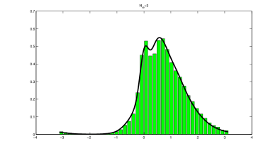
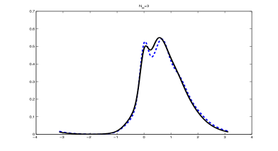
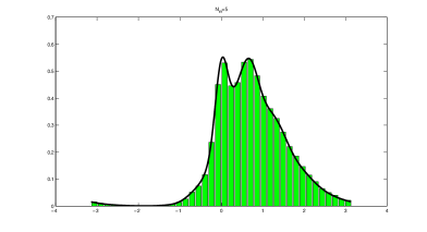
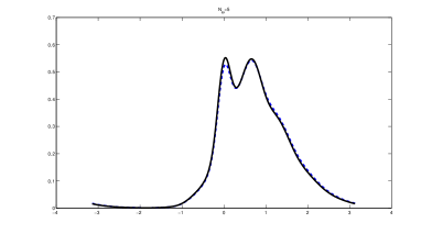
Figure 1: Left. Result of the data fitting with $N_{\Theta}=3$ rates. Histograms: experimental Lévy data collected in $40$ bins. Solid line calculated PDF. Right. Dashed line calculated PDF with the original $5$ rates.

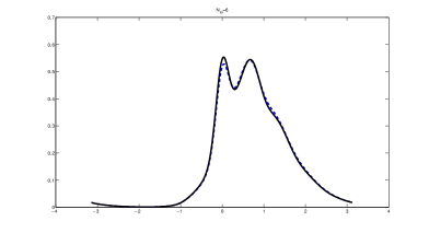
Figure 2: Result of the data fitting with $N_{\Theta}=5$ rates. Histograms: experimental Lévy data collected in $40$ bins. Solid line calculated PDF. Right. Dashed line calculated PDF with the original $5$ rates.

Figure 3: Result of the data fitting with $N_{\Theta}=6$ rates. Histograms: experimental Lévy data collected in $40$ bins. Solid line calculated PDF. Right. Dashed line calculated PDF with the original $5$ rates.

Another interesting problem is the selection of the number of parameters $N_{\Theta}$ and the corresponding basis functions $\Theta_{j}$ for the best data fit. In Fig. 4 we depict the result of the Akaike’s Information Criterion (AIC) [13], given by

$$AIC(N_{\Theta})=LJ(f,\bar{\alpha}^{*})-\log(N_{\Theta}).$$ (50)

A common choice in statistics is to pick that parametrization that maximises the AIC. We can see that criterion gives the value $N_{\Theta,opt}=6$, while the correct value is $5$. The difference in the AIC is however rather small for $N_{\Theta}$ between 5 and 7.

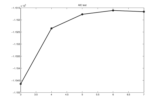
Figure 4: Test for the appropriate regularisation with Akaike’s Information Criterion

Fitting Data from a bi-directional gamma process.

In the second test we fit the final position at $T=1$ of $10^{5}$ samples of a stochastic process with the jumps distributed according a bi-directional gamma process with Lévy measure $\nu$ on $\mathbb{R}$ given by the density [2]

$$d\nu(s)=A\frac{e^{-\beta|s|}}{|s|}ds.$$ (51)

Here $A>0$ is the so-called shape parameter and $\beta$ is the rate parameter. Note that this is not a finite measure, so we are out of the compound Poisson class, and the trajectory of the bidirectional gamma process as infinitely many (small) jumps. In [2] only the unidirectional Gamma process is described. Let $Y^{+}(t)$ be such a unidirectional gamma process, then the Lévy measure is

$$d\nu_{+}(s)=A\frac{e^{-\beta s}}{s}1_{\{s>0\}}(s)ds\mbox{ and }f_{Y^{+}(t)}(y)=\frac{\beta^{At}}{\Gamma(At)}y^{At-1}e^{-\beta y}1_{\{y>0\}}(y).$$ (52)

Let thus $Y^{+}(t)$ and $Y^{-}(t)$ be two independent copies of the Gamma process, then

$$Y(t)=Y^{+}(t)-Y^{-}(t)$$ (53)

is our bi-directional gamma process, which is the jump part of our Lévy process that also includes diffusion as in the first experiment. If we project $Y(t)$ to the torus $[-\pi,\pi]$, the effect on the projected Levy measure $\phi_{*}\nu$, see (2), of the projected Lévy process $X(t)=\phi(Y(t))$ is

$$d\phi_{*}\nu(s)=\left(\sum_{n=0}^{\infty}A\frac{e^{-\beta(|s|+n\pi)}}{|s|+n\pi}\right)ds=\frac{A}{\pi}e^{-\beta|s|}\left(\sum_{n=0}^{\infty}\frac{e^{-\beta\pi n}}{\frac{|s|}{\pi}+n}\right)ds.$$ (54)

Using

$$\sum_{n=0}^{\infty}\frac{e^{-qc}}{p+n}=e^{-q}\Phi(e^{-q},1,p),~{}~{}p\not=0,q>0,$$ (55)

with $\Phi(z,s,a)$ the Lerch transcendent, for $p=|s|/\pi$ and $q=\beta\pi$, we get

$$d\phi_{*}\nu(s)=\frac{A}{\pi}e^{-\beta(|s|+\pi)}\Phi\left(e^{-\beta\pi},1,\frac{|s|}{\pi}\right)ds$$ (56)

as the Lévy measure on the torus for the projected bi-directional Gamma process.

In the simulations data are generated by scaling the rate parameter such that $1/\beta=1$, and setting the shape to $A=0.5$. Finally, the data $Y(t)$ are projected to the torus $[-\pi,\pi)$. In Fig. 5 we report the result of the AIC test the fit with $N_{\Theta}=9$ basis functions centered to $\theta_{j}=(-1+2(j-1)/9)\pi,j=1,\ldots 9$, whose the calculated rates are $\bar{\alpha}=(0,0.0417,0.0235,0.1529,0.8827,0.8616,0.1517,0.0316,0.0396)$. We conclude that our procedure results in high quality fits, even for Lévy distributions that are not part of our hierarchy of parametrizations, but can only be approximated by these.

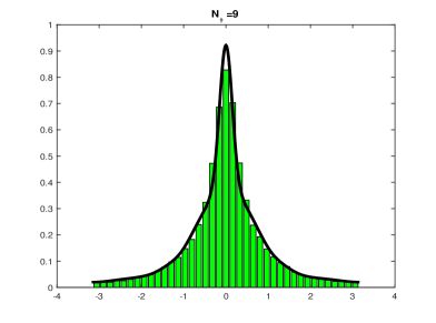
Figure 5: Left, AIC test for the Gamma test. Right, fit with $N_{\Theta}=9$ basis functions.

Financial Data.

As an example from a real world problem we report the result of fitting of the German Stock Exchange (DAX) index, which is publicly available, e.g. from the Yahoo Finance, see Figure 6 left panel. Within the data of all closing quotes between April 1998 and March 2015, there are several periods of elevated volatility, so called volatility bursts. Obviously, this contradicts the description of the market with an exponential levy model $S(t)=e^{Y(t)}$ [2, 15, 24], as the statistical law of $Y(t)-Y(s)$ does not only depend on $t-s$. In order to avoid the pitfalls of time dependent (or stochastic [15, 24]) volatility, we identify a period of comparatively stable volatility of 1000 trading days between April 1998 and February 2002, see the right panel of Figure 6. This data set has a small drift value $b=6.787\times 10^{-4}$ which corresponds to the increased value of the stocks of 67% nominal interest rate in 1000 trading days (followed by severe losses in the subsequent period). The empirical daily volatility (i.e. standard deviation of daily log-returns) in this period of time is $\sigma=9.304\times 10^{-3}$. The obvious absence of axial symmetry prohibits a Gaussian (Black-Scholes) market model from the outset. Our goal is to find a suitable description of this sample with an exponential Lévy market model from our hierarchy of parametrizations.

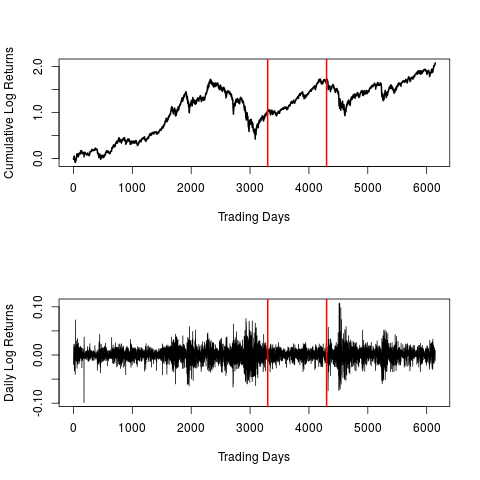
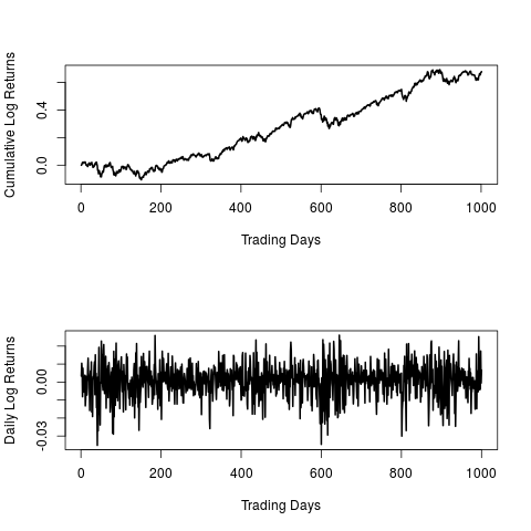
Figure 6: Cumulative and daily log-returns of the DAX index between 26/11/1990 and 05/03/2015 (left panel) 16/4/1998 and 4/02/2002 (right panel). The vertical lines on the left panel correspond to the time period on the right panel, downloaded from finance.yahoo.com

The data has been mapped to the $[-\pi,\pi]$ torus, by rescaling and ’wrapping’ the daily log-Returns below/above 3%, i.e. $[\Omega_{a},\Omega_{b}]=[-0.03,0.03]$. Three data sets, all of them negative, were situated outside this band . The drift value is adapted to a re-scaled torus $[-\pi,\pi)$. Thus the drift on the torus of length $2\pi$ is $b=6.787\times 10^{-4}\pi/0.03=0.07017$.

One fourth of the total empirical variance $8.655\cdot 10^{-5}$ is attributed for the ’fixed’ diffusion, compare Section 2, which yields a coefficient for the Laplace operator equals to $\pi^{2}\mbox{(empirical Variance)}/(0.03)^{2}/4/2=0.2372$ on the torus rescaled to $[-\pi,\pi)$.

With this setting we calculated the fitting of the distribution, with equally spaced basis functions in the interval $[-\pi,\pi)$. In Fig. 7 (left panel) we report the result of the AIC test and the fit with $N_{\Theta}=6$ (right panel). The selected basis functions are centred at $\theta_{j}=(-1+(j-1)/3)\pi,j=1,\ldots 6$, whose the calculated rates are $\bar{\alpha}=(0,0,0.484,0.223,0.304,0)$. Although only three parameters are different from zero, the AIC is maximized at $N_{\Theta}=6$. That the AIC at $N_{\Theta}=3$ is lower is explained by the fact, that the more localized basis functions in the $N_{\Theta}=6$-basis are more adequate to fit the data. It is also a misinterpretation that the chosen parametrization misses an effective description with three parameters, since the position of the grid points are additional parameters. Note that the zero entries of the 1st, 2nd and 6th slot $\bar{\alpha}$ actually correspond to small positive values and only represented as zero when rounded to the 3rd digit.

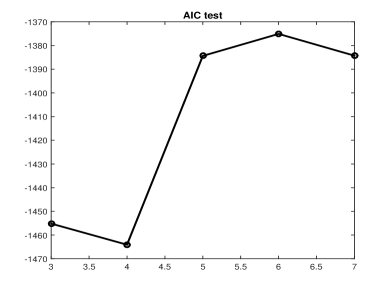
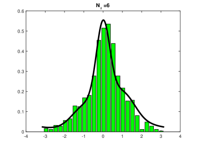
Figure 7: Left, AIC for the maximum likelihood estimate as a function of parameters for the DAX data (left). Right density for the Maximum-Likelihood fit with $N_{\Theta}=6$ basis functions, corresponding to the maximal AIC.

6 Conclusion and Outlook

In the present article, we demonstrate the use of optimal control for PIDE for the non parametric estimation of Lévy processes. Here the PIDE is given by Kolmogorov’s forward equation which allows one to calculate the terminal distribution of the Lévy process at time $T$. The objective functional is the log-likelihood evaluated on a sample of terminal values of the Lévy process.

Based on the study of Lévy distributions, we set up approximate estimation problems that can be tackled by maximum likelihood estimation along with model selection based on Akaike’s information criterion (AIC). As the density of Lévy probability distributions in most cases can not be determined analytically, numerical solutions of the Kolmogorov forward equation (Fokker-Planck equation) and its backward (adjoint) analogue are needed for the efficient maximization of the log-likelihood functional.

For the numerical solution of the optimality system we used the Chang-Cooper method with a mid-point quadrature rule and second order backward time differentiation formula. This numerical scheme is second order accurate and conservative, and we found conditions for stability and positivity of the numerical solution. We use a non linear conjugate gradient method to find the optimality condition.

We have shown that this method works for spline discretizations of the density of the Lévy measure with symmetric boundary conditions for up to 11 parameters. The results consistently fit simulated data from the family of discretizations itself. The same turns out to be true from Lévy processes that only can be approximated by such discretizations, if the number of parameters goes to infinity, like the gamma process. Here the AIC provides an effective mechanism to choose an adequate discretization at a given sample size. Finally, we have demonstrated that also real-world, financial data can be effectively fitted using our strategy.

The future potential of this solution lies in the fact that, unlike FFT / spectral based calibration procedures that are widely used in financial engineering [7, 15, 24], the present approach naturally generalizes to processes that originate as the solution of Stochastic Differential Equations (SDE) with state dependent coefficients. Such local volatility models are frequently used in contemporary financial engineering.

In this work, we used historic and low frequency data for non parametric model calibration. High frequency historical data and implicit volatility data [15, 24] are natural candidates to set up new objective functionals for related control problems that go beyond the control of the terminal distribution.

Another relevant problem is the notorious occurrence of local minima in the maximum likelihood estimation. We expect this to be more severe, when the number of parameters significantly increases. An interesting hybrid approach would combine the robustness of non-parametric spectral calibration methods as a sort of pre-conditioner with the highly efficient maximum likelihood estimation.

Acknowledgements: We would like to thank Alfio Borzi for interesting discussions and hospitality at the University of Würzburg.

References

- [1] D.N. Allen, R.V. Southwell, Relaxation methods applied to determine the motion, in 2-D, of a viscous fluid past a fixed cylinder, Quart-J. Mech. Appl. VIII, 2 (1955) 129-145.
- [2] D. Applebaum, Lévy Processes and Stochastic Calculus, Cambridge University Press, Cambridge, 2004.
- [3] M. Annunziato, A. Borzì, Optimal control of probability density functions of stochastic processes, Math. Model. and Analysis, 15 (2010) 393–407.
- [4] M. Annunziato, A. Borzì, A Fokker-Planck control framework for multidimensional stochastic processes, J. of Comp. and App. Math., 237 (2013) 487–507.
- [5] M. Annunziato, A. Borzì, F. Nobile, R. Tempone, On the Connection between the Hamilton-Jacobi-Bellman and the Fokker-Planck Control Frameworks. Appl. Mathematics, 5 (2014) 2476–2484.
- [6] H. Bauer, Probability Theory, (translated edition) De Gruyter 1995.
- [7] D. Belomestny, M. Reiß, Spectral Calibration of Exponential Lévy Models, Finance Stoch 10 (2006) 449-474.
- [8] G. Berg, C. Forst, Potential Theory on Locally Compact Abelian Groups, Springer Berlin - Heidelberg - New York, 1975.
- [9] D. Bertsekas, Dynamic Programming and Optimal Control, Vols. I and II, Athena Scientific, 2007.
- [10] M. Briani, R. Natalini, G. Russo, Implicit-explicit numerical schemes for jump-diffusion processes, Calcolo 44 (2007) 33–57.
- [11] M. Mohammadi, A. Borzì, Analysis of the Chang-Cooper discretization scheme for a class of Fokker-Planck equations. Journal of Numerical Mathematics (2014). to appear.
- [12] A. Borzi, V. Schulz, Computational Optimization of Systems Governed by Partial Differential Equations, SIAM, Philadephia 2012.
- [13] K. P. Burnham, D. R. Anderson, Model Selection and Multimodel Inference: A Practical Information-Theoretic Approach. Springer, New York, 2002.
- [14] J.S. Chang, G. Cooper, A practical scheme for Fokker-Planck equations, J. Comput. Phys. 6 (1970) 1–16.
- [15] R. Cont, P. Takov, Financial Modeling with Jump Processes, Chapman & Hall, Boca Raton - London - New York - Washington D.C., 2004.
- [16] R. Cont, E. Voltchkova, A finite difference scheme for option pricing in jump diffusion and exponential Lévy models, SIAM J. Numer. Anal. 43 (2005) 1596–1626.
- [17] Y.H. Dai, Y. Yuan, A nonlinear conjugate gradient with a strong global convergence property, SIAM J. Optim. 10 (1999) 177–182.
- [18] Daniel J. Duffy, Numerical Analysis of Jump Diffusion Models: A Partial Differential Equation Approach, Wilmott Magazine (2009) 68–73.
- [19] T. S. Fergusson, A Course in Large Sample Theory, Chapman & Hall, Boca Raton - London - New York - Washington D.C., 1996.
- [20] T. L. Friesz, Dynamic Optimization and Differential Games, Springer New York - Dortrecht - Heidelberg - London 2010.
- [21] S. Geman, C.-H. Hwang, non-parametric Maximum Likelihood Estimation by the Method of Sieves, Ann. of Statistics 10, No. 2 (1982) 401-414.
- [22] H. Gottschalk, B. Smii, H. Thaler, The Feynman graph representation for the convolution semigroup and its applications to Lévy statistics, Bernoulli 14, No. 2 (2008), 322-351.
- [23] J.C. Gilbert, J. Nocedal, Global convergence properties of conjugate gradient methods for optimization, SIAM J. Optim. 2 (1992), 21–42.
- [24] S. Iacus, Option Pricing and Estimation of Financial Models with R, Wiley, Chichester, 2011.
- [25] J. Nocedal, S.J. Wright, Numerical Optimization, Springer, New York, 1999.
- [26] L. A. Sakhonovich, Lévy Processes, Integral Equations, Statistical Physics: Connections and Interactions, Birkhäuser, Basel, 2012.
- [27] R.J. Plemmons, M-matrix characterizations. I-nonsingular M-matrices, Linear Algebra and its Applications. 18 No. 2 (1977) 175–188.
- [28] D. L. Scharfetter and H. K. Gummel, Large signal analysis of a silicon Read diode, IEEE Trans. Electron. Dev., 16 (1969) 64–77.
- [29] D.F. Shanno, Conjugate gradient methods with inexact searches, Math. Oper. Res. 3 (1978) 244–256.