Large-scale optimization-based non-negative
computational framework for diffusion equations:
Parallel implementation and performance studies
   
An e-print of the paper is available on arXiv: 1506.08435.

Authored by

J. Chang

Graduate Student, University of Houston.

S. Karra

Staff Scientist, Los Alamos National Laboratory.

K. B. Nakshatrala

Department of Civil & Environmental Engineering
University of Houston, Texas 77204–4003.
phone: +1-713-743-4418, e-mail: knakshatrala@uh.edu
website: http://www.cive.uh.edu/faculty/nakshatrala

This figure shows the fate of chromium after 180 days using the single-field Galerkin formulation. The white regions indicate the violation of the non-negative constraint.

Abstract.

It is well-known that the standard Galerkin formulation, which is often the formulation of choice under the finite element method for solving self-adjoint diffusion equations, does not meet maximum principles and the non-negative constraint for anisotropic diffusion equations. Recently, optimization-based methodologies that satisfy maximum principles and the non-negative constraint for steady-state and transient diffusion-type equations have been proposed. To date, these methodologies have been tested only on small-scale academic problems. The purpose of this paper is to systematically study the performance of the non-negative methodology in the context of high performance computing (HPC). PETSc and TAO libraries are, respectively, used for the parallel environment and optimization solvers. For large-scale problems, it is important for computational scientists to understand the computational performance of current algorithms available in these scientific libraries. The numerical experiments are conducted on the state-of-the-art HPC systems, and a single-core performance model is used to better characterize the efficiency of the solvers. Our studies indicate that the proposed non-negative computational framework for diffusion-type equations exhibits excellent strong scaling for real-world large-scale problems.

1. INTRODUCTION

The modeling of flow and transport in subsurface is vital for energy, climate and environmental applications. Examples include CO₂ migration in carbon-dioxide sequestration, enhanced geothermal systems, oil and gas production, radio-nuclide transport in a nuclear waste repository, groundwater contamination, and thermo-hydrology in the Arctic permafrost due to the recent climate change [15, 23, 10, 17]. Several numerical codes (e.g., FEHM [40], TOUGH [37], PFLOTRAN [22]) have been developed to model flow and transport in subsurface at reservoir-scale. These codes typically solve unsteady Darcy equations for flow and advection-diffusion equation for transport. The predictive capability of a numerical simulator depends on the robustness of the underlying numerical methods. A necessary and essential requirement is to satisfy important mathematical principles and physical constraints. One such property in transport and reactive-transport problems is that the concentration of a chemical species cannot be negative. Mathematically, this translates to the satisfaction of the discrete maximum principle (DMP) for diffusion-type equations. Subsurface flow and transport applications typically encounter geological media that are highly heterogeneous and anisotropic in nature, and it is well-known that the classical finite element (or finite volume and finite difference, for that matter) formulations do not produce non-negative solutions on arbitrary meshes for such porous media [6, 24, 35, 32].

Several studies over the years have focused on the development of methodologies that enforce the DMP and ensure non-negative solutions [35, 32, 36, 33]. However, these studies did not address how these methods can be used for realistic large-scale subsurface problems that have millions of grid nodes. Furthermore, complex coupling between different physical processes as well as the presence of multiple species amplify the degrees-of-freedom (i.e., the number of unknowns). The aim of this paper is to develop a parallel computational framework that solves anisotropic diffusion equations on general meshes, ensures non-negative solutions, and can be employed to solve large-scale realistic problems.

Large-scale problems can be tackled by using recent advancements in high-performance computing (HPC) methods and toolkits that can be used on the state-of-the-art supercomputing architecture. One such toolkit is PETSc [3], which provides data structures and subroutines for setting up structured and unstructured grids, parallel communication, linear and non-linear solvers, and parallel I/O. These high-level data structures and subroutines help in faster development of parallel application codes and minimize the need to program low-level message passing, so that the domain scientists can focus more on the application. To this end, we develop a non-negative parallel framework by leveraging the existing capabilities within PETSc. Our framework ensures the DMP for anisotropic diffusion by using lower-order finite elements and the optimization-based approach in [35, 24, 32]. The TAO toolkit [31], which is built on top of PETSc, is used for solving the resulting optimization problems. The robustness of the proposed framework will be demonstrated by solving realistic large-scale problems.

The rest of this paper is organized as follows. In Section 2, we present the governing equations and the classical single-field Galerkin finite element formulation for steady-state and transient diffusion equations. The optimization-based method to ensure non-negative concentrations is also outlined in this section. In Section 3, the parallel implementation procedure using PETSc and TAO is presented. We also highlight the relevant data structures used in this study and present a pseudo algorithm describing our parallel framework. In Section 4, a performance model loosely based on the roofline model is outlined. This model is used to estimated the efficiency with respect to computing hardware of currently available solvers within PETSc and TAO. In Section 5, we first verify our implementation using a 3D benchmark problem from the literature and present a detailed performance study using the proposed model. Then, we study a large-scale three-dimensional realistic problem involving the transport of chromium in the subsurface and document the numerical results of the non-negative methodology with the classical single-field Galerkin formulation. Conclusions are drawn in Section 6.

2. GOVERNING EQUATIONS AND ASSOCIATED NON-NEGATIVE NUMERICAL METHODOLOGIES

Let $\Omega\subset\mathbb{R}^{nd}$ be a bounded open domain, where “$nd$” is the number of spatial dimensions. The boundary of the domain is denoted by $\partial\Omega=\overline{\Omega}-\Omega$, which is assumed to be piecewise smooth. A spatial point is denoted by $\mathbf{x}\in\overline{\Omega}$. The gradient and divergence operators with respect to $\mathbf{x}$ are, respectively, denoted as $\mathrm{grad}[\cdot]$ and $\mathrm{div}[\cdot]$. As usual, the boundary is divided into two parts: $\Gamma^{\mathrm{D}}$ and $\Gamma^{\mathrm{N}}$. $\Gamma^{\mathrm{D}}$ is that part of the boundary on which Dirichlet boundary conditions are prescribed, and $\Gamma^{\mathrm{N}}$ is the part of the boundary on which Neumann boundary conditions are prescribed. For mathematical well-posedness, we assume $\Gamma^{\mathrm{D}}\cup\Gamma^{\mathrm{N}}=\partial\Omega$ and $\Gamma^{\mathrm{D}}\cap\Gamma^{\mathrm{N}}=\emptyset$. The unit outward normal to boundary is denoted as $\widehat{\mathbf{n}}(\mathbf{x})$. The diffusivity tensor is denoted by $\mathbf{D}(\mathbf{x})$, which is assumed to symmetric, bounded above and uniformly elliptic. That is,

$$\mathbf{D}(\mathbf{x})=\mathbf{D}^{\mathrm{T}}(\mathbf{x})\quad\forall\mathbf{x}\in\Omega$$ (2.1)

and there exists two constants $\mathrm{0<\xi_{1}\leq\xi_{2}<+\infty}$ such that

$$\xi_{1}\mathbf{y}^{\mathrm{T}}\mathbf{y}\leq\mathbf{y}^{\mathrm{T}}\mathbf{D}(\mathbf{x})\mathbf{y}\leq\xi_{2}\mathbf{y}^{\mathrm{T}}\mathbf{y}\quad\forall\mathbf{x}\in\Omega\;\mathrm{and}\;\forall\mathbf{y}\in\mathbb{R}^{nd}$$ (2.2)

2.1. Governing equations for steady-state response

We shall denote the steady-state concentration field by $c(\mathbf{x})$. The governing equations can be written as follows:

$$- \mathrm{div}[\mathbf{D}(\mathbf{x})\mathrm{grad}[c]]=f(\mathbf{x}) \mathrm{in}\;\Omega$$ (2.3a)

$$c(\mathbf{x})=c^{\mathrm{p}}(\mathbf{x}) \mathrm{on}\;\Gamma^{\mathrm{D}}$$ (2.3b)

$$- \mathbf{\widehat{n}}(\mathbf{x})\cdot\mathbf{D}(\mathbf{x})\mathrm{grad}[c]=q^{\mathrm{p}}(\mathbf{x}) \mathrm{on}\;\Gamma^{\mathrm{N}}$$ (2.3c)

where $f(\mathbf{x})$ is the volumetric source/sink, $c^{\mathrm{p}}(\mathbf{x})$ is the prescribed concentration, and $q^{\mathrm{p}}(\mathbf{x})$ is the prescribed flux. For uniqueness, we assume $\Gamma^{\mathrm{D}}\neq\emptyset$.

2.1.1. Maximum principle and the non-negative constraint

The above boundary value problem is a self-adjoint second-order elliptic partial differential equation (PDE). It is well-known that such PDEs possess an important mathematical property – the classical maximum principle [8]. The mathematical statement of the classical maximum principle can be written as follows: If $c(\mathbf{x})\in C^{2}(\Omega)\cap C^{0}(\overline{\Omega})$, $\partial\Omega=\Gamma^{\mathrm{D}}$, and $f(\mathbf{x})\leq 0$ in $\Omega$ then

$$\max_{\mathbf{x}\in\overline{\Omega}}c(\mathbf{x})=\max_{\mathbf{x}\in\partial\Omega}c^{\mathrm{p}}(\mathbf{x})$$ (2.4)

Similarly, if $f(\mathbf{x})\geq 0$ in $\Omega$ then

$$\min_{\mathbf{x}\in\overline{\Omega}}c(\mathbf{x})=\min_{\mathbf{x}\in\partial\Omega}c^{\mathrm{p}}(\mathbf{x})$$ (2.5)

To make our presentation on maximum principles simple, we have assumed stronger regularity on the solution (i.e., $c(\mathbf{x})\in C^{2}\cap C^{0}(\overline{\Omega})$), and assumed that Dirichlet boundary conditions are prescribed on the entire boundary. However, maximum principles requiring milder regularity conditions on the solution, even for the case when Neumann boundary conditions are prescribed on the boundary, can be found in literature (see [30, 29]).

If $f(\mathbf{x})\geq 0$ in $\Omega$ and $c^{\mathrm{p}}(\mathbf{x})\geq 0$ on the entire $\partial\Omega$ then the maximum principle implies that $c(\mathbf{x})\geq 0$ in the entire domain, which is the non-negativity of the concentration field.

2.1.2. Single-field Galerkin weak formulation

The following function spaces will be used in the rest of this paper:

$$\mathcal{U} :=\left\{c(\mathbf{x})\in H^{1}(\Omega)\;\big{|}\;c(\mathbf{x})=c^{\mathrm{p}}(\mathbf{x})\;\mathrm{on}\;\Gamma^{\mathrm{D}}\right\}$$ (2.6)

$$\mathcal{W} :=\left\{w(\mathbf{x})\in H^{1}(\Omega)\;\big{|}\;w(\mathbf{x})=0\;\mathrm{on}\;\Gamma^{\mathrm{D}}\right\}$$ (2.7)

where $H^{1}(\Omega)$ is a standard Sobolev space [1]. The single-field Galerkin weak formulation corresponding to equations (2.3a)–(2.3c) reads: Find $c(\mathbf{x})\in\mathcal{U}$ such that we have

$$\mathcal{B}(w;c)=L(w)\quad\forall w(\mathbf{x})\in\mathcal{W}$$ (2.8)

where the bilinear form and linear functional are, respectively, defined as

$$\mathcal{B}(w;c) :=\int_{\Omega}\mathrm{grad}[w(\mathbf{x})]\cdot\mathbf{D}(\mathbf{x})\mathrm{grad}[c(\mathbf{x})]\;\mathrm{d}\Omega$$ (2.9a)

$$L(w) :=\int_{\Omega}w(\mathbf{x})f(\mathbf{x})\;\mathrm{d}\Omega+\int_{\Gamma^{\mathrm{N}}}w(\mathbf{x})q^{\mathrm{p}}(\mathbf{x})\;\mathrm{d}\Gamma$$ (2.9b)

Since $\mathbf{D}(\mathbf{x})$ is symmetric, by Vainberg’s theorem [13], the single-field Galerkin weak formulation given by equation (2.8) is equivalent to the following variational problem:

$$\mathop{\mathrm{minimize}}_{c(\mathbf{x})\in\mathcal{U}}\quad\frac{1}{2}\mathcal{B}(c;c)-L(c)$$ (2.10)

2.1.3. A methodology to enforce the maximum principle for steady-state problems

Our methodology is based on the finite element method. We decompose the domain into “$Nele$” non-overlapping open element sub-domains such that

$$\overline{\Omega}=\bigcup_{e=1}^{Nele}\overline{\Omega}^{e}$$ (2.11)

(Recall that a superposed bar denotes the set closure.) The boundary of $\Omega^{e}$ is denoted by $\partial\Omega^{e}:=\overline{\Omega}^{e}-\Omega^{e}$. We shall define the following finite dimensional vector spaces of $\mathcal{U}$ and $\mathcal{W}$:

$$\mathcal{U}^{h} :=\left\{c^{h}(\mathbf{x})\in\mathcal{U}\;\big{|}\;c^{h}(\mathbf{x})\in C^{0}(\overline{\Omega}),c^{h}(\mathbf{x})\big{|}_{\Omega^{e}}\in\mathbb{P}^{k}(\Omega^{e}),e=1,\cdots,Nele\right\}$$ (2.12a)

$$\mathcal{W}^{h} :=\left\{w^{h}(\mathbf{x})\in\mathcal{W}\;\big{|}\;w^{h}(\mathbf{x})\in C^{0}(\overline{\Omega}),w^{h}(\mathbf{x})\big{|}_{\Omega^{e}}\in\mathbb{P}^{k}(\Omega^{e}),e=1,\cdots,Nele\right\}$$ (2.12b)

where $k$ is a non-negative integer, and $\mathbb{P}^{k}(\Omega^{e})$ denotes the linear vector space spanned by polynomials up to $k$-th order defined on the sub-domain $\Omega^{e}$. The finite element formulation for equation (2.8) can be written as: Find $c^{h}(\mathbf{x})\in\mathcal{P}^{h}$ such that we have

$$\mathcal{B}(q^{h};c^{h})=L(q^{h})\quad\forall q^{h}(\mathbf{x})\in\mathcal{Q}^{h}$$ (2.13)

It has been documented in the literature that the above finite element formulation violates the maximum principle and the non-negative constraint [24, 35, 32].

We now outline an optimization-based methodology that satisfies the maximum principle and the non-negative constraint on general computational grids. To this end, we shall use the symbols $\preceq$ and $\succeq$ to denote component-wise inequalities for vectors. That is, for given any two vectors $\boldsymbol{a}$ and $\boldsymbol{b}$

$$\boldsymbol{a}\preceq\boldsymbol{b}\quad\mbox{means that }\quad a_{i}\leq b_{i}\;\forall i$$ (2.14)

The symbol $\succeq$ can be similarly defined as well. Let $<\cdot;\cdot>$ denote the standard inner-product in Euclidean space. After finite element discretization, the discrete equations corresponding to equation (2.13) take the form

$$\boldsymbol{K}\boldsymbol{c}=\boldsymbol{f}$$ (2.15)

where $\boldsymbol{K}$ is a symmetric positive definite matrix, $\boldsymbol{c}$ is the vector containing nodal concentrations, and $\boldsymbol{f}$ is the force vector. Equation (2.15) is equivalent to the following minimization problem

$$\mathop{\mbox{minimize}}_{\boldsymbol{c}\in\mathbb{R}^{ndofs}}\quad\frac{1}{2}\langle\boldsymbol{c};\boldsymbol{K}\boldsymbol{c}\rangle-\langle\boldsymbol{c};\boldsymbol{f}\rangle$$ (2.16)

where “$ndofs$” denotes the number of degrees of freedom for concentration. Equation (2.15) can lead to unphysical negative solutions.

Following [32, 24], a methodology corresponding to equation (2.16) that satisfies the non-negative constraint can be written as follows:

$$\mathop{\mbox{minimize}}_{\boldsymbol{c}\in\mathbb{R}^{ndofs}}\quad\frac{1}{2}<\boldsymbol{c};\boldsymbol{K}\boldsymbol{c}>-<\boldsymbol{c};\boldsymbol{f}>$$ (2.17a)

$$\mbox{subject to}\quad\boldsymbol{0}\preceq\boldsymbol{c}$$ (2.17b)

where $\boldsymbol{0}$ is a vector of size $ndofs$ containing zeros. Since $\boldsymbol{K}$ is positive definite, equation (2.17) has a unique global minimum [4]. Several robust numerical methods can be used to solve equation (2.17), which include active set strategy, interior point methods [4]. In this paper, to solve the resulting optimization problems, we shall use the parallel optimization toolkit TAO [31], which has the active-set Newton trust region (TRON) and quasi-Newton-based bounded limited memory variable metric (BLMVM) algorithms.

2.2. Governing equations for transient response

We shall denote the time by $t\in[0,\mathcal{I}]$, where $\mathcal{I}$ denotes the length of the time interval of interest. We shall denote the time-dependent concentration by $c(\mathbf{x},t)$. The initial boundary value problem can be written as follows:

$$\frac{\partial c}{\partial t}=\mathrm{div}[\mathbf{D}(\mathbf{x})\mathrm{grad}[c]]+f(\mathbf{x},t) \quad\mathrm{in}\;\Omega\times(0,\mathcal{I})$$ (2.18a)

$$c(\mathbf{x},t)=c^{\mathrm{p}}(\mathbf{x},t) \quad\mathrm{on}\;\Gamma^{\mathrm{D}}\times(0,\mathcal{I})$$ (2.18b)

$$- \widehat{\mathbf{n}}(\mathbf{x})\cdot\mathbf{D}(\mathbf{x})\mathrm{grad}[c]=q^{\mathrm{p}}(\mathbf{x},t) \quad\mathrm{on}\;\Gamma^{\mathrm{N}}\times(0,\mathcal{I})$$ (2.18c)

$$c(\mathbf{x},0)=c_{0}(\mathbf{x}) \quad\mathrm{in}\;\Omega$$ (2.18d)

where $c_{0}(\mathbf{x})$ is the prescribed initial concentration, $f(\mathbf{x},t)$ is the time-dependent volumetric source/sink, $c^{\mathrm{p}}(\mathbf{x},t)$ is the time-dependent prescribed concentration on the boundary, and $q^{\mathrm{p}}(\mathbf{x},t)$ is the prescribed time-dependent flux on the boundary.

2.2.1. Maximum principle and the non-negative constraint

The maximum principle of a transient diffusion equation asserts that the maximum can occur only on the boundary of the domain or in the initial condition if $f(\mathbf{x},t)\leq 0$ and $\Gamma^{\mathrm{D}}=\partial\Omega$. Mathematically, a solution to equations (2.18a)–(2.18a) will satisfy:

$$c(\mathbf{x},t)\leq\max\left[\max_{\mathbf{x}\in\Omega}c_{0}(\mathbf{x}),\max_{\mathbf{x}\in\partial\Omega}c^{\mathrm{p}}(\mathbf{x},t)\right]\quad\forall t$$ (2.19)

provided $f(\mathbf{x},t)\leq 0$. Similarly, the minimum will occur either on the boundary or in the initial condition if $f(\mathbf{x},t)\geq 0$. That is, if $f(\mathbf{x},t)\geq 0$ then a solution to equations (2.18a)–(2.18a) satisfies:

$$c(\mathbf{x},t)\geq\min\left[\min_{\mathbf{x}\in\Omega}c_{0}(\mathbf{x}),\min_{\mathbf{x}\in\partial\Omega}c^{\mathrm{p}}(\mathbf{x},t)\right]\quad\forall t$$ (2.20)

If $f(\mathbf{x},t)\geq 0$ in $\Omega$, $c^{\mathrm{p}}(\mathbf{x},t)\geq 0$ on the entire $\partial\Omega$, and $c_{0}(\mathbf{x})\geq 0$ in $\Omega$ then the maximum principle implies that $c(\mathbf{x},t)\geq 0$ in the entire domain at all times, which is the non-negative constraint for the concentration field for transient problems.

2.2.2. A methodology to enforce the maximum principle for transient problems

We divide the time interval of interest into $\mathcal{N}$ sub-intervals. That is,

$$[0,\mathcal{I}]:=\bigcup_{n=0}^{\mathcal{N}}[t_{n},t_{n+1}]$$ (2.21)

where $t_{n}$ denotes the $n$-th time-level. We assume that the time-step is uniform, which can be written as:

$$\Delta t=t_{n+1}-t_{n}$$ (2.22)

Following the recommendation provided in [34] to meet maximum principles, we employ the backward Euler method for temporal discretization. We shall denote the nodal concentrations at the $n$-th time-level by $\boldsymbol{c}^{(n)}$. We shall denote the minimum and maximum values for the concentration by $c_{\mathrm{min}}$ and $c_{\mathrm{max}}$, which will be provided by the maximum principle and the non-negative constraint. At each time-level, one has to solve the following convex quadratic program:

$$\mathop{\mathrm{minimize}}_{\boldsymbol{c}^{(n+1)}}\quad\frac{1}{2}\langle{\boldsymbol{c}^{(n+1)}};\widetilde{\boldsymbol{K}}\boldsymbol{c}^{(n+1)}\rangle-\langle{\boldsymbol{c}^{(n+1)}};\widetilde{\boldsymbol{f}}^{(n+1)}\rangle$$ (2.23a)

$$\mbox{subject to}\quad c_{\mathrm{min}}\mathbf{1}\preceq\boldsymbol{c}^{(n+1)}\preceq c_{\mathrm{max}}\mathbf{1}$$ (2.23b)

where

$$\widetilde{\boldsymbol{K}}:=\frac{1}{\Delta t}\boldsymbol{M}+\boldsymbol{K}$$ (2.24)

$$\widetilde{\boldsymbol{f}}^{(n+1)}:=\boldsymbol{f}^{(n+1)}+\frac{1}{\Delta t}\boldsymbol{M}\boldsymbol{c}^{(n+1)}$$ (2.25)

In the above equation, $\boldsymbol{M}$ is the capacity matrix [34].

3. PARALLEL IMPLEMENTATION

3.1. PETSc and TAO

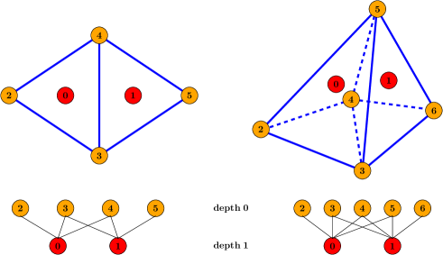
(a) Optimal 2D and 3D elements

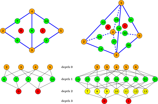
(b) Interpolated 2D and 3D elements

Figure 1. Representation of mesh points within the DMPlex data structure and their associated directed acyclic graphs

We leverage on existing scientific libraries such as PETSc and TAO to formulate our large-scale computational framework. PETSc is a suite of data structures and routines for the parallel solution of scientific applications. It also provides interfaces to several other libraries such as Metis/ParMETIS[16] and HDF5 [38] for mesh partitioning and binary data format handling respectively. The Data Management (DM) data structure is used to manage all information including vectors and sparse matrices and compatible with binary data formats. To handle unstructured grids in parallel, a subset of the DM structure called DMPlex (see [21, 20, 3]), as shown in Figure 1, uses the direct acyclic graph to organize all mesh information. This topology enables the freedom to mix and match various non vertex-based discretization such as the two-point flux finite volume method and the classical mixed formulations based on the lowest-order Raviart Thomas finite element space.

Another important feature within PETSc is TAO. The TAO library has a suite of data structures and routines that enable the solution of large-scale optimization problems. It can support any data structure or solver within PETSc. Our non-negative methodology will use both the Newton-Trust Region (TRON) and Bounded Limited-Memory Variable-Metric (BLMVM) solvers available within TAO. BLMVM is a quasi-Newton method that uses projected gradients to approximate the Hessian, which is useful for problems where the hessian is too complicated or expensive to compute. Other optimization algorithms such as TRON and the Gradient Projected Conjugate Gradient (GPCG) typically require Hessian information and more memory, but they are expected to converge more rapidly than BLMVM. Further details regarding the implementation of these various methods may be found in [31] and the references within.

3.2. Finite element implementation

PETSc abstractions for finite elements, quadrature rules, and function spaces have also been recently introduced and are suitable for the mesh topology within DMPlex. They are built upon the same framework as the Finite element Automatic Tabulator (FIAT) found within the FEniCS Project [18, 26, 27]. The finite element discretizations simply need the equations, auxiliary coefficients (e.g., permeability, diffusivity, etc.), and boundary conditions specified as point-wise functions. We express all discretizations in nonlinear form so let $\boldsymbol{r}$ and $\boldsymbol{J}$ denote the residual and Jacobian respectively.

Following the FEM model outlined in [19], we consider the weak form that depends on fields and gradients. The residual evaluation can be expressed as:

$$\boldsymbol{w}^{\mathrm{T}}\boldsymbol{r}(\boldsymbol{c})\sim\int_{\Omega^{e}}\left[w\cdot\mathcal{F}_{0}\left(c,\nabla c\right)+\nabla w\cdot\boldsymbol{\mathcal{F}}_{1}(c,\nabla c)\right]\mathrm{d}\Omega=0$$ (3.1)

where $\mathcal{F}_{0}(c,\nabla c)$ and $\boldsymbol{\mathcal{F}}_{1}(c,\nabla c)$ are user-defined point-wise functions that capture the problem physics. This framework decouples the problem specification from the mesh and degree of freedom traversal. That is, the scientist need only focus on providing point function evaluations while letting the finite element library take care of meshing, quadrature points, basis function evaluation, and mixed forms if any. The discretization of the residual is written as:

$$\boldsymbol{r}(\boldsymbol{c})=\mathop{\huge\boldsymbol{\mathsf{A}}}_{e=1}^{Nele}\left[\begin{array}[]{lr}\boldsymbol{N}^{\mathrm{T}}&\boldsymbol{B}^{\mathrm{T}}\end{array}\right]\boldsymbol{W}\left[\begin{array}[]{l}\mathcal{F}_{0}(c_{q},\nabla c_{q})\\ \boldsymbol{\mathcal{F}}_{1}(c_{q},\nabla c_{q})\end{array}\right]$$ (3.5)

where $\boldsymbol{\mathsf{A}}$ represents the standard assembly operator, $\boldsymbol{N}$ and $\boldsymbol{B}$ are matrix forms of basis functions that reduce over quadrature points, $\boldsymbol{W}$ is a diagonal matrix of quadrature weights (including the geometric Jacobian determinant of the element), and $c_{q}$ is the field value at quadrature point $q$. The Jacobian of (3.5) needs only the derivatives of the point-wise functions:

$$\boldsymbol{J}(\boldsymbol{c})=\mathop{\huge\boldsymbol{\mathsf{A}}}_{e=1}^{Nele}\left[\begin{array}[]{lr}\boldsymbol{N}^{\mathrm{T}}&\boldsymbol{B}^{\mathrm{T}}\end{array}\right]\boldsymbol{W}\left[\begin{array}[]{ll}\mathcal{F}_{0,0}&\mathcal{F}_{0,1}\\ \boldsymbol{\mathcal{F}}_{1,0}&\boldsymbol{\mathcal{F}}_{1,1}\end{array}\right]\left[\begin{array}[]{c}\boldsymbol{N}\\ \boldsymbol{B}\end{array}\right],\quad\left[\mathcal{F}_{i,j}\right]=\left[\begin{array}[]{ll}\frac{\partial\mathcal{F}_{0}}{\partial c}&\frac{\partial\mathcal{F}_{0}}{\partial\nabla c}\\ \frac{\partial\boldsymbol{\mathcal{F}}_{1}}{\partial c}&\frac{\partial\boldsymbol{\mathcal{F}}_{1}}{\partial\nabla c}\end{array}\right](c_{q},\nabla c_{q})$$ (3.13)

The point-wise functions corresponding to the weak form in (2.9) would be:

Create/input DAG on rank 0

Create/input cell-wise velocity on rank 0

if size $>$ 1 then

     Partition mesh among all processors

end if

Refine distributed mesh if necessary

Create PetscSection and FE discretization

Set $n=0$ and $\boldsymbol{c}^{(0)}=10^{-8}$

Insert Dirichlet BC constraints into $\boldsymbol{c}^{(0)}$

Compute Jacobian $\boldsymbol{J}$

while true do $\triangleright$ Begin time-stepping scheme

     Compute Residual $\boldsymbol{r}^{(n)}$

     if Classical Galerkin then $\triangleright$ Solve without non-negative methodology

         $\boldsymbol{c}^{(n+1)}=\boldsymbol{c}^{(n)}-\boldsymbol{J}\backslash\boldsymbol{r}^{(n)}$

     else$\triangleright$ Solve with non-negative methodology

         TaoSolve() for $\boldsymbol{c}^{(n+1)}$ based on equations (3.18) and (3.19)

     end if

     if steady-state or $(n)==$ total number of time steps then

         break

     else

         $n+=1$

     end if

end while

Algorithm 1 Pseudocode for the large-scale transport solver

$$\mathcal{F}_{0}=-f(\mathbf{x}),\quad\boldsymbol{\mathcal{F}}_{1}=\mathbf{D}(\mathbf{x})\nabla c_{q}$$ (3.14a)

$$\mathcal{F}_{0,0}=0,\quad\mathcal{F}_{0,1}=0,\quad\boldsymbol{\mathcal{F}}_{1,0}=\mathbf{0},\quad\boldsymbol{\mathcal{F}}_{1,1}=\mathbf{D}(\mathbf{x})$$ (3.14b)

Similarly, the point-wise functions for the transient response are:

$$\mathcal{F}_{0}=\dot{c}_{q}-f(\mathbf{x},t),\quad\boldsymbol{\mathcal{F}}_{1}=\mathbf{D}(\mathbf{x})\nabla c_{q}$$ (3.15a)

$$\mathcal{F}_{0,0}=\frac{1}{\Delta t},\quad\mathcal{F}_{0,1}=0,\quad\boldsymbol{\mathcal{F}}_{1,0}=\mathbf{0},\quad\boldsymbol{\mathcal{F}}_{1,1}=\mathbf{D}(\mathbf{x})$$ (3.15b)

where $\dot{c}_{q}$ denotes the time derivative. A similar discretization is used to project the Neumann boundary conditions into the residual vector. Assuming a fixed time-step, $[\mathcal{F}_{i,j}]$ and the Jacobian in equation (3.13) do not change with time and have to be computed only once. If $n$ denotes the time level ($n$ = 0 denotes initial condition) then the residual and Jacobian can be defined as:

$$\boldsymbol{r}^{(n)}\equiv\boldsymbol{r}(\boldsymbol{c}^{(n)})$$ (3.16)

$$\boldsymbol{J}\equiv\boldsymbol{J}(\boldsymbol{c}^{(0)})$$ (3.17)

To enforce the non-negative methodology, the following objective function $b$ and gradient function $\boldsymbol{g}$ is provided:

$$b=\frac{1}{2}\boldsymbol{c}^{(n+1)}\cdot\boldsymbol{J}\boldsymbol{c}^{(n+1)}+\boldsymbol{c}^{(n+1)}\cdot\left[\boldsymbol{r}^{(n)}-\boldsymbol{J}\boldsymbol{c}^{(n)}\right]$$ (3.18)

$$\boldsymbol{g}=\boldsymbol{J}\left[\boldsymbol{c}^{(n+1)}-\boldsymbol{c}^{(n)}\right]+\boldsymbol{r}^{(n)}$$ (3.19)

BLMVM relies only on the above two equations, whereas TRON needs the Hessian which is equivalent to $\boldsymbol{J}$. Algorithm 1 outlines the steps taken in our computational framework.

4. PERFORMANCE MODELING

PETSc is a constantly evolving open-source library that brings out new features and algorithms almost every day. It has capabilities to interface with a large number of other open-source software and linear algebra packages. However, it is not always known which of these algorithms will have the best performance across multiple distributed memory HPC systems, especially if these packages have little documentation and have to be used as black-box solvers. Computational scientists would like to know which solvers or algorithms to use for their specific need before running jobs on the state-of-the-art HPC systems. The first and the trivial metric to look for in answering this question is the time-to-solution for a given solver or optimization method. However, additional information is needed in order to quantify the hardware and algorithmic efficiency as well as the potential scalability across multiple cores in the strong sense.

Table 1. List of HPC systems used in this study

	Mustang (MU)	Wolf (WF)
Processor	AMD Opteron 6176	Intel Xeon E5-2670
Clock rate	2.3 GHz	2.6 GHz
FLOPs/cycle	4	8
Sockets per compute node	2	2
NUMA nodes per socket	2	1
Cores per socket	12	8
Total cores (compute nodes)	38400 (1600)	9856 (616)
Memory per compute node	64 GB	64 GB
L1 cache per core	128 KB	32 KB
L2 cache per core	512 KB	256 KB
L3 cache per socket	12 MB	20 MB
Interconnect	40 Gb/s	40 Gb/s

Hardware specifications of HPC systems significantly impact the performance of any numerical algorithm. Ideally we want our simulations to consume as little wall-clock time as possible as the number of processing cores increases (i.e., achieving good speedup), but several other factors including compiler vectorization, cache locality, memory bandwidth, and code implementation may drastically affect the performance. Table 1 lists the hardware specifications of the two HPC systems (Mustang and Wolf) that are used in our numerical experiments. The Mustang HPC system consists of relatively older generation of processors so it is expected to not perform as well. One could simply measure wall-clock time across multiple compute nodes on the respective HPC machines and determine the parallel efficiency of a certain algorithm, but we are interested in quantifying how different algorithms behave sequentially and what kind of parallel performance to expect before running numerical simulations on supercomputers. The wall-clock time of any simulation can generally be summed up as a function of three things: the workload, transfer of data between the memory and CPU register, and interprocess communication. Hardware efficiency in this context is defined as the amount of time spent performing work over waiting on memory fetching and cache registers to free up.

The limiting factor of performance for numerical methods on modern computing architectures is upper-bounded by the memory bandwidth. That is, the floating point performance given by FLOPS/s will never reach the theoretical peak performance (TPP). This limitation is particularly important for iterative solvers and optimization methods that rely on numerous sparse matrix-vector (SpMV) multiplications (see [28] and the references within). The frequent use of SpMV allows for little cache reuse and will result in a large number of very expensive cache misses. Such behavior is important to document when determining how efficient a scientific code is, so performance models such as the Roofline Model [39, 25], which measures memory transfers, have been used to better quantify the efficiency with respect to the hardware. Performance models in general can help application developers identify bottlenecks and indicate which areas of the code can be further optimized. In other words, the code can be designed so that it maximizes the full benefits of the available computing resources. In the next section, we will demonstrate that such models can also be used to predict the parallel efficiency of various optimization solvers on the two very different LANL HPC systems. The key parameter for these performance models is the Arithmetic Intensity (AI) which is defined as:

$$\mbox{AI}=\frac{\mbox{Total FLOPS}}{\mbox{Total Bytes Transferred}}$$ (4.1)

where the Total Bytes Transferred (TBT) metric denotes the amount of bandwidth needed for a given floating point operation. The AI serves as a multiplier to the actual memory bandwidth and creates a “roofline” for the estimation of ideal peak performance. A cache model is needed in order to properly define the TBT.

Table 2. Commonly used PETSc operations and their respective Total Bytes Transferred. Here we note $X,Y,Z$ as vectors with $i=1,\cdots,N$ entries, $a$ is a scalar value, and $nz$ denotes the total number of non-zeros. We assume that the sizes of integers and doubles are 4 and 8 bytes respectively.

PETSc function	Operation	Total Bytes Transferred
VecNorm()	$a=\sqrt{\sum^{N}_{i}X(i)^{2}}$	$8(N+1)$
VecDot()	$a=\sum^{N}_{i}X(i)*Y(i)$	$8(2N+1)$
VecCopy()	$Y\leftarrow X$	$8(2N)$
VecSet()	$Y(i)=a$	$8(2N)$
VecScale()	$Y=a*Y$	$8(2N)$
VecAXPY()	$Y=a*X+Y$	$8(3N)$
VecAYPX()	$Y=X+a*Y$	$8(3N)$
VecPointwiseMult()	$Z(i)=X(i)*Y(i)$	$8(3N)$
MatMult()	SpMV	$4(N+nz)+8(2N+nz)$

To this end, we propose a roofline-like performance model where the TBT assumes a “perfect cache” – each byte of the data needs to be fetched from DRAM only once. This assumption enables us to predict a slightly more realistic upper bound of the peak performance than by simply comparing to the TPP. Table 2 lists the key PETSc functions used for the solvers and their respective estimates of TBT based on the perfect cache assumption. The formula for SpMV follows the procedure outlined in [9]. We assume that the TBT formula for operations also involving a sparse matrix and vector like the incomplete lower-upper (ILU) factorization to be the same as MatMult(). Estimating the TBT for other important operations like the sparse matrix-matrix and triple matrix products (which are important for multi-grid methods) is an area of future work. In short, our AI formulation relies on the following four key assumptions:

1. All floating-point operations (add, multiply, square roots, etc.) are treated equally and equate to one FLOP count.

2. There are no conflict misses. That is, each matrix and vector element is loaded into cache only once.

3. Processor never waits on a memory reference. That is, any number of loads and stores are satisfied in a single cycle.

4. Compilers are capable of storing scalar multipliers in the register only for pure streaming computations.

Therefore, the efficiency based on this new roofline-like performance model as:

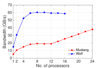
(a)

Figure 2. Estimated memory bandwidth of a single Mustang and Wolf compute node based on the STREAMS Triad Benchmark

$$\mbox{Efficiency (\%)}=\frac{\mbox{Measured FLOPS/s}}{\mathrm{min}\left\{\begin{array}[]{l}\mbox{TPP}\\ \mathrm{AI}\times\mbox{STREAMS}\end{array}\right.}\times 100$$ (4.4)

where the numerator is reported by the PETSc program and the denominator is the ideal performance upper-bounded by both the TPP and the product of AI and STREAMS bandwidth. STREAMS Triad [14] is one of the most popular benchmarks for determining the achievable memory performance of a given machine. Figure 2 denotes the estimated memorybandwidth as a function of number of cores on a single Mustang and Wolf node. It is interesting to note that although the Wolf node has a greater bandwidth, there is no performance gain past eight cores. This means that an optimal use of a Wolf compute node for memory-bandwidth bound algorithms would be eight cores, whereas one would still see some performance gains when using all 24 cores on a Mustang node.

The performance model that uses equation (4.4) is a serial model so the STREAMS metric for the Mustang and Wolf systems are 5.65 GB/s and 15.5 GB/s respectively. It should be noted that this performance model does account for cache effects. That is, it does not quantify the useful bandwidth sustained for some level of cache. The true hardware and algorithmic efficiency is not be reflected by this model, so our aim is to show relative performance between select PETSc and TAO solvers. Comparing the AI and the measured FLOPS/s with the STREAMS bandwidth will give us a better understanding of how high-performing the PETSc and TAO solvers are for select problems.

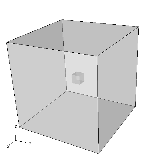
(a) Location of the hole

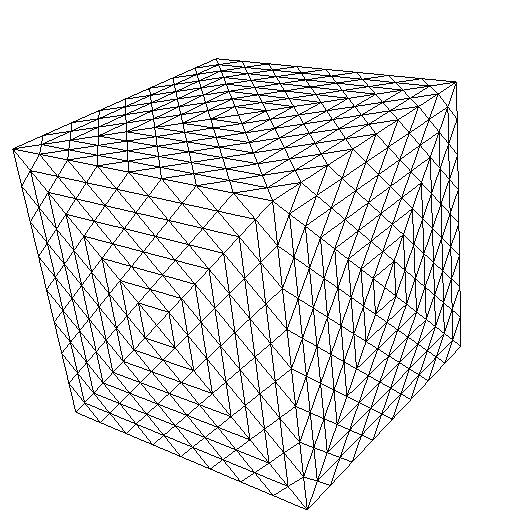
(b) Mesh type A

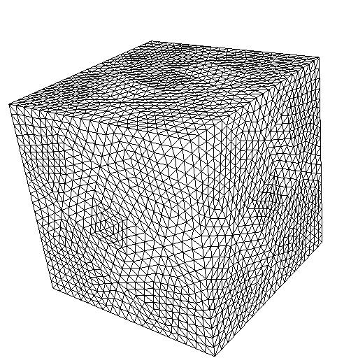
(c) Mesh type B

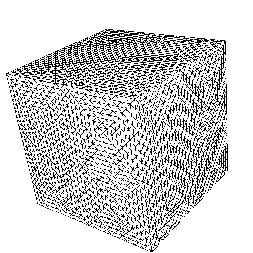
(d) Mesh type C

Figure 3. Cube with a hole: pictorial description and the associated unstructured grids.

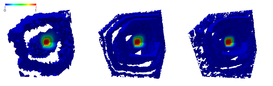
(a)

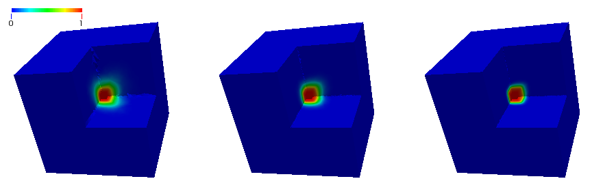
(b)

Figure 4. Cube with a hole: numerical solution for cases A1 (left), B2 (middle), and C3 (right) using the Galerkin formulation (top row) and non-negative methodology (bottom row).

5. REPRESENTATIVE NUMERICAL RESULTS

In this section, we compare the performance of our non-negative methodology using the TAO solver to that of the Galerkin formulation using the Krylov Subspace (KSP) solver. We examine the performance using two problems:

1. a unit cube with a hole under steady-state, and

2. a transient Chromium transport problem.

The diffusivity tensor is assumed to depend on the flow velocity through

$$\mathbf{D}(\mathbf{x})=\left(\alpha_{T}\|\mathbf{v}\|+D_{M}\right)\mathbf{I}+(\alpha_{L}-\alpha_{T})\frac{\mathbf{v}\otimes\mathbf{v}}{\|\mathbf{v}\|}$$ (5.1)

where $\alpha_{L}$, $\alpha_{T}$, and $D_{M}$ denote the longitudinal dispersivity, transverse dispersivity and molecular diffusivity, respectively. We employ the conjugate gradient method and the block Jacobi/ILU(0) preconditioner for solving the linear system from the Galerkin formulation and employ TAO’s TRON and BLMVM methods for the non-negative methodology. The relative convergence tolerances for both KSP and TAO solvers are set to $10^{-6}$, and $\Delta t$ for the transient response in the Chromium problem is initially set to 0.2 days. For strong-scaling studies shown here, we used OpenMPI v1.6.5 for message passing and bound processes to cores while mapping by sockets. ParaView[2] and VisIt[5] were used to generate all contour and mesh plots.

Remark 1.

Throughout the paper, the non-negative methodology that we refer to, is in fact a discrete maximum principle preserving methodology, in that, along with the non-negative constraint we also enforce that the concentrations are less than or equal to 1.

5.1. Anisotropic diffusion in a unit cube with a cubic hole

Let the computational domain be a unit cube with a cubic hole of size $[4/9,5/9]\times[4/9,5/9]\times[4/9,5/9]$. The concentration on the outer boundary is taken to be zero and the concentration on the interior boundary is taken to be unity. The volumetric source is taken as zero (i.e., $f(\mathbf{x})=0$). The velocity vector field for this problem is chosen to be

$$\mathbf{v}(\mathbf{x})=\mathbf{e}_{x}+\mathbf{e}_{y}+\mathbf{e}_{z}$$ (5.2)

Table 3. Cube with a hole: list of various mesh type and refinement level combinations used

Case	Mesh type	Refinement level	Tetrahedrons	Vertices
A1	A	1	199,296	36,378
B1	B	1	409,848	75,427
C1	C	1	793,824	140,190
A2	A	2	1,594,368	278,194
B2	B	2	3,278,784	574,524
C2	C	2	6,350,592	1,089,562
A3	A	3	12,754,994	2,175,330
B3	B	3	26,230,272	4,483,126
C3	C	3	50,804,736	9,172,044

Table 4. Cube with a hole: minimum and maximum concentrations for each case

Case	Min. concentration	Max. concentration	% nodes violated
A1	-0.0224825	1.00000	9,518/36,378 $\rightarrow$ 26.2%
B1	-0.0139559	1.00000	32,247/43,180 $\rightarrow$ 42.8%
C1	-0.0125979	1.00000	57,272/140,190 $\rightarrow$ 40.9%
A2	-0.0311518	1.00103	82,983/278,194 $\rightarrow$ 29.2%
B2	-0.0143857	1.00000	255,640/574,524 $\rightarrow$ 44.9%
C2	-0.0119539	1.00972	453,766/1,089,562 $\rightarrow$ 41.6%
A3	-0.0258559	1.00646	643,083/2,175,330 $\rightarrow$ 29.6%
B3	-0.0115908	1.00192	2,073,934/4,483126 $\rightarrow$ 46.3%
C3	-0.0096186	1.00545	4,932,551/9,172,044 $\rightarrow$ 53.8%

Table 5. Cube with a hole: wall-clock times (seconds) on Mustang for each solver

Case	Galerkin	TRON1	TRON2	TRON3	BLMVM
A1	0.337	0.933	0.981	1.14	2.62
B1	0.790	1.72	2.06	2.71	5.04
C1	2.24	4.34	5.80	7.74	13.5
A2	7.21	15.2	21.7	32.5	72.0
B2	15.4	30.0	43.7	57.5	109
C2	40.4	67.8	113	118	286
A3	121	225	414	599	1167
B3	315	498	1061	1344	2524
C3	997	1539	2490	4365	9679

Table 6. Cube with a hole: wall-clock times (seconds) on Wolf for each solver

Case	Galerkin	TRON1	TRON2	TRON3	BLMVM
A1	0.126	0.388	0.396	0.449	1.01
B1	0.314	0.720	0.853	1.07	2.03
C1	0.888	1.91	2.47	3.31	5.71
A2	2.58	6.34	8.74	12.8	26.2
B2	5.90	12.9	17.8	22.8	46
C2	16.2	30.1	47.3	48.9	133
A3	48.0	98.4	129	247	609
B3	107	171	342	435	1060
C3	281	467	870	1245	3131

The diffusion parameters are set as: $\alpha_{L}=1$, $\alpha_{T}=0.001$, and $D_{M}=0$. The pictorial description of the computational domain and the three mesh types composed of 4-node tetrahedrons are shown in Figure 3. We consider three unstructured mesh types with three levels of element-wise mesh refinement, giving us nine total case studies of increasing problem size as shown in Table 3. We ran a total of five different simulations for this study:

• Galerkin with CG/block Jacobi

• TRON1: with KSP tolerance of $10^{-1}$

• TRON2: with KSP tolerance of $10^{-2}$

• TRON3: with KSP tolerance of $10^{-3}$

• BLMVM

The TRON solvers also use the CG and block Jacobi preconditioner but with different KSP tolerances. Numerical results for both the Galerkin formulation and the non-negative methodologies for some of the mesh cases are shown in Figure 4. The top row of figures arise from the Galerkin formulation where the white regions denote negative concentrations, and the bottom row arise from either TRON or BLMVM. Details concerning the violation of the DMP for each case study can be found in Table 4. Concentrations both negative and greater than one arise for all case studies. Moreover, simply refining the mesh does not resolve these issues; in fact, refinment worsens the violation. These numerical results indicate that our computational framework can successfully enforce the DMP for diffusion problems with highly anisotropic diffusivity.

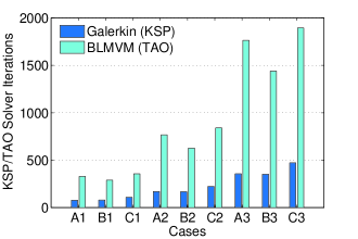
(a)

Figure 5. Cube with a hole: solver iterations needed for Galerkin and BLMVM.

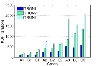
(a)

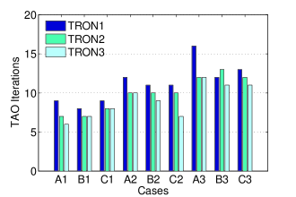
(b)

Figure 6. Cube with a hole: KSP (left) and TAO (right) solver iterations needed for TRON.

5.1.1. Performance modeling

We first consider the wall-clock time spent in the solvers on a single core. Table 5 and 6 depict the solver time for each mesh, and we first note that Mustang system requires significantly more wall-clock time to obtain a solution than Wolf; this behavior is expected due to the difference in HPC hardware specifications listed in Table 1, specifically, Mustang has the lower clock rate and lower bandwidth (as determined through STREAMS Triad). It can also be seen that the various non-negative solvers consume varying amounts of wall-clock time. BLMVM can require as much as ten times the amount of wall-clock time as the standard Galerkin method. TRON on the other hand, does not consume nearly as much time but tightening the KSP tolerances will gradually increase the amount of time. We are interested in determine why these optimization solvers consume more wall-clock time, whether it be mostly due to additional workload associated with optimization-based techniques or due to the presence of relatively more complicated and expensive data structures compared to the standard solvers used for the Galerkin formulation. The first step is noting the total KSP and TAO iterations needed and how they vary with respect to problem size. Figure 5 depicts the KSP and TAO iterations for the Galerkin and BLMVM methods respectively. It is well-known that block Jacobi (also known as ILU(0)) requires more iterates as the size of the problem increases. In other words, the solver may exhibit poor scaling for extremely large problems, but we see that the BLMVM algorithm has an even poorer scaling rate of the solver iterates. For the TRON solvers, we document both the KSP and TAO iterates as shown in Figure 6. We see that tightening the KSP tolerance increases the number of KSP iterates but requires slightly fewer TAO iterates. This behavior indicates that the more accurate the computed gradient projection is, the fewer optimization loops the solver has to perform.

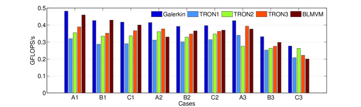
(a) Mustang

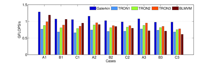
(b) Wolf

Figure 7. Cube with a hole: measured floating-point rate (FLOPS/s) on a single core.

(a)

Figure 8. Cube with a hole: arithmetic intensity for all solvers and all cases on a single processor.

We also examine the measured floating-point rate provided by the PETSc performance logs, as shown in Figure 7, of all five solvers across their respective machines, and the floating point performance decreases as the problem size grows. One could compare these numbers to the TPP and see that the hardware efficiencies are no greater than $5\%$, but it is difficult to draw any other conclusions with regard to the computational performance. The calculated AI, based on our proposed performance model, is shown in Figure 8. It is interesting to note that the AI remains largely invariant with problem size unlike the wall-clock time, solver iterations, and floating point rates. According to the perfect cache model, the Galerkin formulation’s AI is greater than any of the non-negative methodologies. The optimization-based algorithm based on TAO’s BLMVM solver has significantly more streaming/vector operations which explains the relatively lower AI. Using these metrics in equation (4.4) as well as the STREAMS Triad bandwidth of one core as shown in Figure 2, the estimated roofline-based efficiencies are shown in Figure 9. Although the raw floating-point rate of BLMVM is lower than the Galerkin method, the roofline model suggests that BLMVM is actually more efficient in the hardware sense. The TRON methods have much lower floating-point rates, but these metrics can be improved or “gamed” by tightening the KSP tolerances. This behavior leads us to believe that there is some latency associated with setting up the data structures needed to compute gradient descent projections.

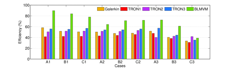
(a) Mustang

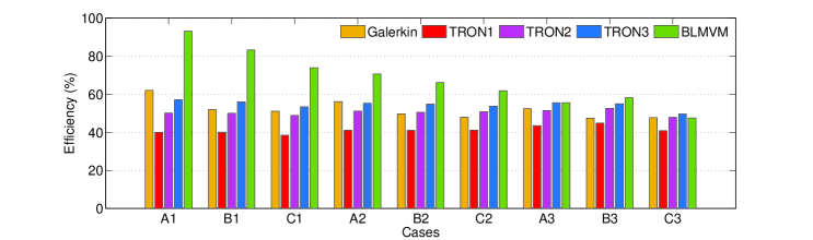
(b) Wolf

Figure 9. Cube with a hole: estimated floating-point efficiency with respect to the arithmetic intensity and measured memory bandwidth from STREAMS.

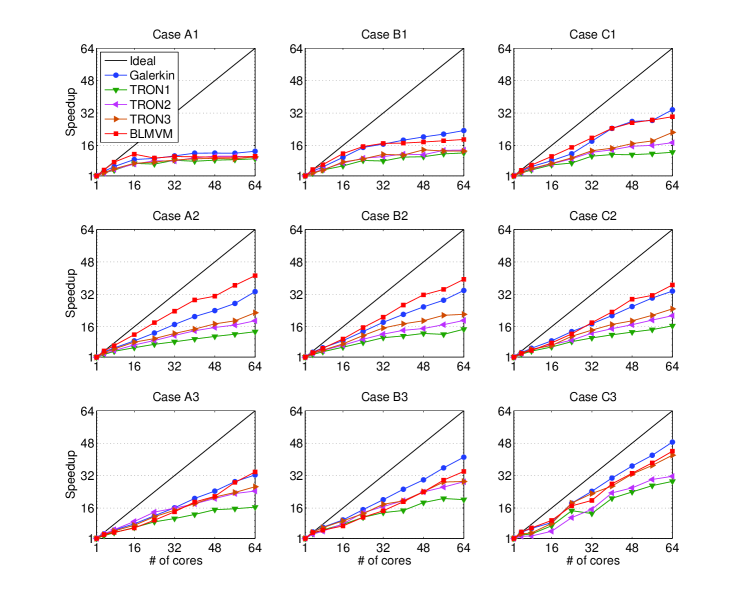
(a)

Figure 10. Cube with a hole: speedup for all 9 mesh cases up to 64 processors on the Mustang system (16 cores per node).

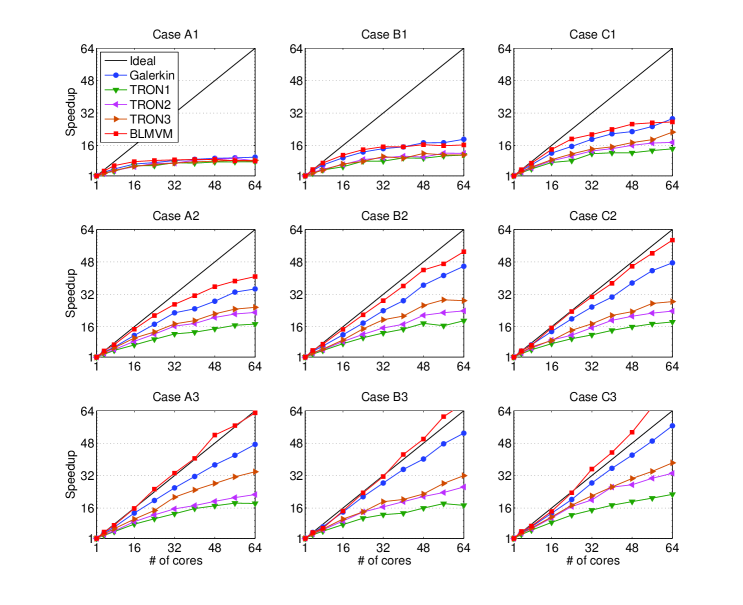
(a)

Figure 11. Cube with a hole: speedup for all 9 mesh cases up to 64 cores on the Wolf system (8 cores per node).

5.1.2. Strong-scaling

The metric of most interest to many computational scientists is the strong-scaling potential of any numerical framework. We conduct strong-scaling studies to measure the speedup of all nine case studies over 64 cores. Four Mustang nodes with 16 cores each and 8 Wolf nodes with 8 cores each are allocated for this study. We do not fully saturate the compute nodes because the STREAMS benchmark indicates that there is little or no gain in memory performance when using a full node. Figure 10 depicts the speedup on the Mustang system, and Figure 11 depicts the speedup on the Wolf system. First, we note that the parallel efficiency (actual speedup over ideal speedup) increases with problem size due to Amdahl’s Law. We also note that Wolf exhibits better strong-scaling due to the faster speedups for the same test studies. For all problems and machines, the TRON simulations are slightly less efficient in the parallel sense but can be improved by tightening the KSP tolerances. Interestingly, the BLMVM algorithm not only has the best roofline efficiency but also the best parallel speedup. We can infer from these results that although BLMVM is the more efficient optimization in the hardware sense, TRON is more efficient in the algorithmic sense due to its lesser time-to-solution. Our study has shown that one can draw correlations between the performance models conducted on a single-core and the actual speedup across multiple distributed memory nodes. As future solvers and algorithms are implemented within PETSc, we can use this performance model to assess how efficient they are in both the hardware and algorithmic sense and how efficiently they will scale in a parallel setting.

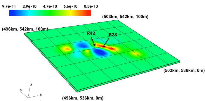
(a)

Figure 12. Chromium plume migration in the subsurface: Permeability field (m²) and the locations of the pumping well (R28) and contaminant source (R42).

5.2. Transport of chromium in subsurface

Table 7. Chromium plume migration in the subsurface: parameters

Parameter	Value
$\alpha_{L}$	100 m
$\alpha_{T}$	0.1 m
Contaminant source (R42)	$1\times 10^{-4}$ kg/m2s2
$\Delta t$	0.2 days
Domain size	7000 km$\times$6000 km$\times$100 m
$D_{M}$	$1\times 10^{-9}$ m2/s
Permeability	Varies
Pumping well (R28)	-0.01 kg/m2s2
Total hexahedrons	1,984,512
Total vertices	2,487,765
$\mathbf{v}$	Varies with position
Viscosity	3.95$\times 10^{-5}$ Pa s

(a)

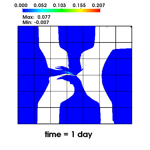
(b)

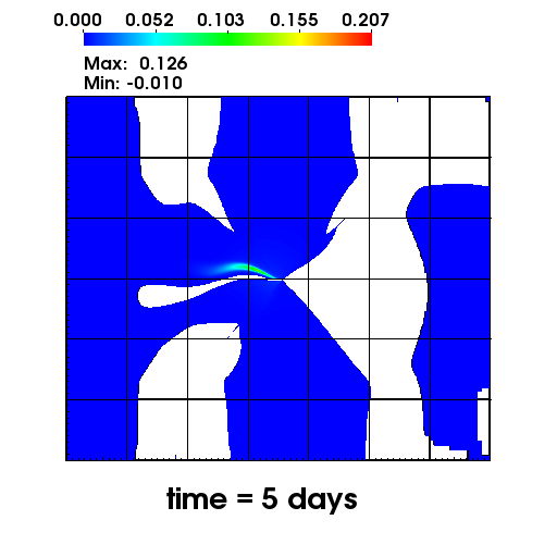
(c)

(d)

(e)

(f)

Figure 13. Chromium plume migration in the subsurface: concentrations at select times using the Galerkin formulation.

(a)

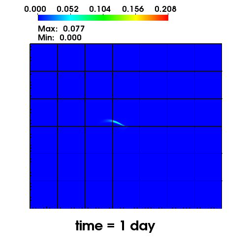
(b)

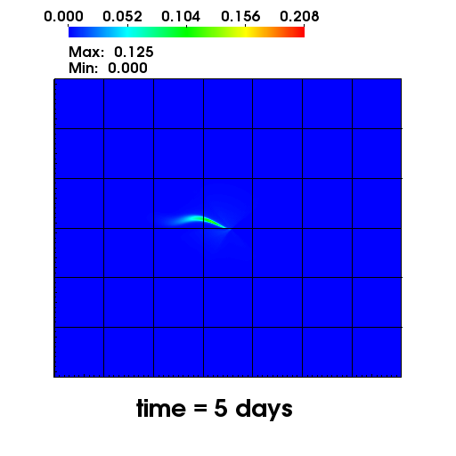
(c)

(d)

(e)

(f)

Figure 14. Chromium plume migration in the subsurface: concentrations at select times using the non-negative methodology.

Subsurface clean-up due to anthropogenic contamination is a big challenge [7]. Remediation studies [10, 11] need accurate predictions of transport of the involved chemical species, which are obtained using limited data at monitoring wells and through numerical simulations. To accurately predict the fate of the contaminant, a transport solver that: a) is robust, in that it will not give unphysical solutions, and b) can handle field-scale scenarios, is needed. The computational framework that is proposed in this paper is an ideal candidate for such problems. We now consider a realistic large-scale problem to predict the fate of chromium in the Los Alamos, New Mexico area. The chromium was released into the Sandia canyon in the 50s up to early 70s. Back then chromium was used as an anti-corrosion agent for the cooling towers at a power plant at the Los Alamos National Laboratory (see [12] and references therein for details).

Here we study the effectiveness of our proposed framework to this real-world scenario of predicting the extent of chromium plume. The following is a conceptual model domain that is considered: A domain of size $[496,503]\mathrm{km}\times[536,542]\mathrm{km}\times[0,100]\mathrm{m}$ with the permeability field (m²) as shown in Figure 12. R42 in Figure 12 is estimated to be the contaminant source location and a pumping well is located at R28. The parameters used for this problem are shown in Table 7, and we employ the following boundary conditions:

$$c^{\mathrm{p}}(x=496\mathrm{km},y,z)=c^{\mathrm{p}}(x=503\mathrm{km},y,z)=c^{\mathrm{p}}(x,y=536\mathrm{km},z)=c^{\mathrm{p}}(x,y=542\mathrm{km},z)=0$$ (5.3)

For this highly heterogeneous problem, we employ PETSc’s algebraic multi-grid preconditioner (GAMG) and couple this with the TRON algorithm for the non-negative solver. Our goal is to examine its strong-scaling potential across 1024 cores. We first solve the steady flow equation (based on mass balance and Darcy’s model to relate pressure and mass flux) with the pumping well located at R28. Cell-wise velocity is obtained from the resulting pressure field and used to calculated element-wise dispersion tensor. We then solve the transient diffusion problem (with tensorial dispersion) with a constant contaminant source located at R40 for up to 180 days. The concentrations at select time levels for Galerkin formulation and non-negative methodology are shown in Figures 13 and 14, respectively. Negative concentrations arise with the Galerkin formulation even as the solution approaches steady-state.

Figure 15 depicts the amount of wall-clock time with respect to the number of cores at the first time level. We see here that the demonstrates good parallel performance across 1024 cores with up to 35 percent parallel efficiency. Unlike the previous benchmark problem, we consider a case where we completely saturate a Wolf node by using all 16 cores and notice that the performance is slightly worse than using a partially saturated node (8 cores). This change of behavior can be attributed to the lack of memory performance improvement one achieves when using all 16 cores as shown in Figure 2. Interprocess communication becomes a major component of the Wolf simulations so the parallel scalability gets worse the more efficiently TRON conducts its work. Nonetheless, the higher quality computing resources of a Wolf node results in faster solve times than the solve time on Mustang even with lesser parallel efficiency.

Another metric of interest is the number of solver iterations required for convergence across various number of MPI processes. Figure 16 depicts the number of KSP solver iterations and TAO solver iterations across 1024 cores, and we notice that there are significant fluctuations. This trend is largely attributed to the accumulation of numerical round-offs from the TRON algorithm. One can reduce these fluctuations by tightening the solver tolerances, but the strong-scaling remains largely unaffected even for the results shown. This study suggests that the proposed non-negative methodology using TRON with GAMG preconditioning is suitable for large-scale transient heterogeneious and anisotropic diffusion equations.

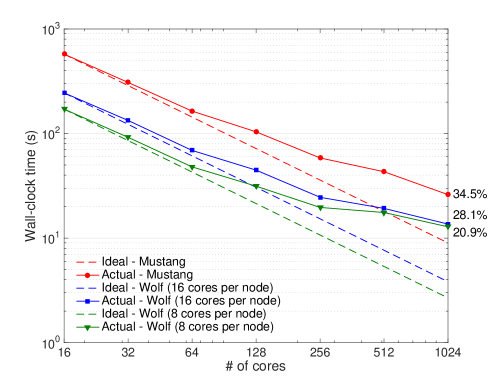
(a)

Figure 15. Chromium plume migration in the subsurface: wall-clock time of the TRON optimization solver with multi-grid preconditioner (GAMG) versus number of processors after the first time level. Two Wolf cases are considered, where we fully saturate a compute node (16 cores) and where we partially saturate a compute node (8 cores per node). The parallel efficiency with respect to 16 cores is shown on the right hand side.

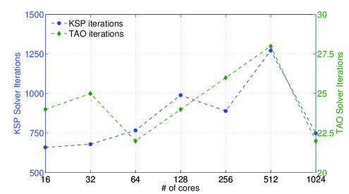
(a)

Figure 16. Chromium plume migration in the subsurface: number of KSP (left hand side) and TAO (right hand side) solver iterations for the TRON optimization solver versus number of cores after the first time level.

6. CONCLUDING REMARKS

We presented a parallel non-negative computational framework suitable for solving large-scale steady-state and transient anisotropic diffusion equations. The main contribution is that the proposed parallel computational framework satisfies the discrete maximum principles for large-scale diffusion-type equations even on general computational grids. The parallel framework is built upon PETSc’s DMPlex data structure, which can handle unstructured meshes, and TAO for solving the resulting optimization problems from the discretization formulation. We have conducted systematic performance modeling and strong-scaling studies to demonstrate the efficiency, both in the parallel and hardware sense of the computational framework. The robustness of the proposed framework has been illustrated by solving a large-scale realistic problem involving the transport of chromium in the subsurface at Los Alamos, New Mexico. Future areas of research include: (a) extending the proposed parallel framework to advective-diffusive and advective-diffusive-reactive systems, and (b) posing the discrete problem as a variational inequality, which will be valid even for non-self-adjoint operators, and use other PETSc capabilities to solve such variational inequalities.

References

- [1] R. J. Adams and J. J. F. Fournier. Sobolev Spaces, volume 140. Academic press, 2003.
- [2] U. Ayachit. The ParaView Guide: A Parallel Visualization Application. Kitware, 2015.
- [3] S. Balay, S. Abhyankar, M. F. Adams, J. Brown, P. Brune, K. Buschelman, V. Eijkhout, W. D. Gropp, D. Kaushik, M. G. Knepley, L. C. McInnes, K. Rupp, B. F. Smith, S. Zampini, and H. Zhang. PETSc users manual. Technical Report ANL-95/11 - Revision 3.6, Argonne National Laboratory, 2015.
- [4] S. Boyd and L. Vandenberghe. Convex Optimization. Cambridge University Press, Cambridge, UK, 2004.
- [5] H. Childs, E. Brugger, B. Whitlock, J. Meredith, S. Ahern, D. Pugmire, K. Biagas, M. Miller, C. Harrison, G. H. Weber, H. Krishnan, T. Fogal, A. Sanderson, C. Garth, E. W. Bethel, D. Camp, O. Rübel, M. Durant, J. M. Favre, and P. Navrátil. VisIt: An End-User Tool For Visualizing and Analyzing Very Large Data. In High Performance Visualization–Enabling Extreme-Scale Scientific Insight, pages 357–372. 2012.
- [6] P. G. Ciarlet and P-A. Raviart. Maximum principle and uniform convergence for the finite element method. Computer Methods in Applied Methods and Engineering, 2:17–31, 1973.
- [7] US EPA. Cleaning up the nation’s waste sites: Markets and technology trends. Technical Report EPA 542-R-04-015, 2004.
- [8] L. C. Evans. Partial Differential Equations. American Mathematical Society, Providence, Rhode Island, USA, 1998.
- [9] W. D. Gropp, D. K. Kaushik, D. E. Keyes, and B. F. Smith. Toward realistic performance bounds for implicit CFD codes. In Proceedings of Parallel CFD ‘99, pages 233–240. Elsevier, 1999.
- [10] G. E. Hammond and P. C. Lichtner. Field-scale model for the natural attenuation of uranium at the Hanford 300 Area using high-performance computing. Water Resources Research, 46:W09602, 2010.
- [11] D. R. Harp and V. V. Vesselinov. Contaminant remediation decision analysis using information gap theory. Stochastic Environmental Research and Risk Assessment, 27(1):159–168, 2013.
- [12] J. M. Heikoop, T. M. Johnson, K. H. Birdsell, P. Longmire, D. D. Hickmott, E. P. Jacobs, D. E. Broxton, D. Katzman, V. V. Vesselinov, M. Ding, D. T. Vanimana, S. L. Reneaua, T. J. Goering, J. Glessnerb, and A. Basu. Isotopic evidence for reduction of anthropogenic hexavalent chromium in Los Alamos National Laboratory groundwater. Chemical Geology, 373:1–9, 2014.
- [13] K. D. Hjelmstad. Fundamentals of Structural Mechanics. Springer Science+Business Media, Inc., New York, USA, second edition, 2005.
- [14] J. McCalpin. STREAM: sustainable memory bandwidth in high performance computers, 1995. https://www.cs.virginia.edu/stream/.
- [15] S. Karra, S. L. Painter, and P. C. Lichtner. Three-phase numerical model for subsurface hydrology in permafrost-affected regions (PFLOTRAN-ICE v1.0). The Cryosphere, 8(5):1935–1950, 2014.
- [16] G. Karypis and V. Kumar. A fast and highly quality multilevel scheme for partitioning irregular graphs. SIAM Journal on Scientific Computing, 20:359–392, 1999.
- [17] S. Kelkar, K. Lewis, S. Karra, G. Zyvoloski, S. Rapaka, H. Viswanathan, P. K. Mishra, S. Chu, D. Coblentz, and R. Pawar. A simulator for modeling coupled thermo-hydro-mechanical processes in subsurface geological media. International Journal of Rock Mechanics and Mining Sciences, 70:569–580, 2014.
- [18] R. C. Kirby. FIAT: Numerical Construction of Finite Element Basis Functions, chapter 13. Springer, 2012.
- [19] M. G. Knepley, J. Brown, K. Rupp, and B. F. Smith. Achieving High Performance with Unified Residual Evaluation. arXiv:1309.1204, September 2013.
- [20] M. G. Knepley and D. A. Karpeev. Mesh algorithms for PDE with vieve I: Mesh distribution. Scientific Programming, 17:215–230, 2009.
- [21] M. Lange, M. G. Knepley, and G. J. Gorman. Flexible, scalable mesh and data management using PETSc DMPlex. In Proceedings of the 3rd International Conference on Exascale Applications and Software, EASC ‘15, pages 71–76. University of Edinburgh, 2015.
- [22] P. C. Lichtner, G. E. Hammond, C. Lu, S. Karra, G. Bisht, B. Andre, R. T. Mills, and J. Kumar. PFLOTRAN user manual: A massively parallel reactive flow and transport model for describing surface and subsurface processes. Technical Report Report No.: LA-UR-15-20403, Los Alamos National Laboratory, 2015.
- [23] P. C. Lichtner and S. Karra. Modeling multiscale-multiphase-multicomponent reactive flows in porous media: Application to CO2 sequestration and enhanced geothermal energy using pflotran. In R. Al-Khoury and J. Bundschuh, editors, Computational Models for CO2 Geo-sequestration & Compressed Air Energy Storage, pages 81–136. CRC Press, http://www.crcnetbase.com/doi/pdfplus/10.1201/b16790-6, 2014.
- [24] R. Liska and M. Shashkov. Enforcing the discrete maximum principle for linear finite element solutions of second-order elliptic problems. Communications in Computational Physics, 3(4):852–877, 2008.
- [25] Y. J. Lo, S. Williams, B. V. Straalen, T. J. Ligocki., M. J. Cordery, N. J. Wright, M. W. Hall, and L. Oliker. Roofline: an insightful visual performance model for multicore architectures. High Performance Computing Systems. Performance Modeling, Benchmarking, and Simulation, 8966:129–148, 2015.
- [26] A. Logg. Efficient Representation of Computational Meshes. International Journal of Computational Science and Engineering, 4:283–295, 2009.
- [27] A. Logg, K. A. Mardal, and G. N. Wells. Automated Solution of Differential Equations by the Finite Element Method. Springer, 2012.
- [28] D. A. May, J. Brown, and L. L. Laetitia. pTatin3D: High-performance methods for long-term lithospheric dynamics. In Proceedings of the International Conference for High Performance Computing, Network, Storage and Analysis, SC ‘14, pages 274–284. IEEE Press, 2014.
- [29] M. K. Mudunuru and K. B. Nakshatrala. On enforcing maximum principles and achieving element-wise species balance for advection-diffusion-reaction equations under the finite element method. Journal of Computational Physics, 305:448–493, 2016.
- [30] M. K. Mudunuru and K. B. Nakshatrala. On mesh restrictions to satisfy comparison principles, maximum principles, and the non-negative constraint: Recent developments and new results. Mechanics of Advanced Materials and Structures, DOI: 10.1080/15502287.2016.1166160, 2016.
- [31] T. Munson, J. Sarich, S. Wild, S. Benson, and L. C. McInnes. TAO 2.0 users manual. Technical Report ANL/MCS-TM-322, Mathematics and Computer Science Division, Argonne National Laboratory, 2012. http://www.mcs.anl.gov/tao.
- [32] H. Nagarajan and K. B. Nakshatrala. Enforcing the non-negativity constraint and maximum principles for diffusion with decay on general computational grids. International Journal for Numerical Methods in Fluids, 67:820–847, 2011.
- [33] K. B. Nakshatrala, M. K. Mudunuru, and A. J. Valocchi. A numerical framework for diffusion-controlled bimolecular-reactive systems to enforce maximum principles and the non-negative constraint. Journal of Computational Physics, 253:278–307, 2013.
- [34] K. B. Nakshatrala, H. Nagarajan, and M. Shabouei. A numerical methodology for enforcing maximum principles and the non-negative constraint for transient diffusion equations. Communications in Computational Physics, 19:53–93, 2016.
- [35] K. B. Nakshatrala and A. J. Valocchi. Non-negative mixed finite element formulations for a tensorial diffusion equation. Journal of Computational Physics, 228:6726–6752, 2009.
- [36] G. S. Payette, K. B. Nakshatrala, and J. N. Reddy. On the performance of high-order finite elements with respect to maximum principles and the nonnegative constraint for diffusion-type equations. International Journal for Numerical Methods in Engineering, 91:742–771, 2012.
- [37] K. Pruess. The TOUGH codes—a family of simulation tools for multiphase flow and transport processes in permeable media. Vadose Zone Journal, 3(3):738–746, 2004.
- [38] The HDF Group. Hierarchical Data Format, version 5, 1997-2015. http://www.hdfgroup.org/HDF5/.
- [39] S. Williams, A. Waterman, and D. Patterson. Roofline: an insightful visual performance model for multicore architectures. Communications of the ACM, 52:65–76, 2009.
- [40] G. Zyvoloski. FEHM: A control volume finite element code for simulating subsurface multi-phase multi-fluid heat and mass transfer. Los Alamos Unclassified Report LA-UR-07-3359, 2007.