IPMU15-0097

Statistics of Flux Vacua for Particle Physics

Taizan Watari

Kavli Institute for the Physics and Mathematics of the Universe, University of Tokyo, Kashiwa-no-ha 5-1-5, 277-8583, Japan

1 Introduction

Flux compactification of F-theory/Type IIB string theory generates discretum of vacua in the complex structure parameter space, making it possible to count vacua and argue statistics of some of observables in the low-energy effective theories [1, 2]. It is virtually impossible to work out the vacuum for each one of individual flux configurations in practice, but this difficulty can be overcome in an approximate treatment of this problem introduced by Ashok–Denef–Douglas [3, 4]. Their treatment becomes a very powerful tool, when used for F-theory compactifications [2, 5], since one can estimate the number of flux vacua that lead to low-energy effective theories with a given set of 7-brane gauge groups and the number of generations of matter fields. It turns out [6] that the number of flux vacua is reduced in the order of $10^{-O(100)}$ generically as we require the rank of 7-brane gauge group to be higher by one. Focusing on an ensemble of flux vacua with a given 7-brane gauge group, one further finds that the number of flux vacua follows the Gaussian distribution on the number of generations $N_{\rm gen}$, with the variance $\left\langle{N_{\rm gen}^{2}}\right\rangle$ not more than O(1).

Obviously the analysis method above can be applied also to more refined and practical problems. It often happens in model building that more than one theoretically and phenomenologically consistent idea (model) has been proposed for a given phenomenon, and one cannot say which is better within the framework of low-energy effective field theory. By counting the number of flux vacua that realise various ideas and comparing the numbers, however, one can introduce a measure of naturalness on those consistent ideas. Such attempts have been made often in Type IIB compactifications so far; we are returning to this program by using F-theory compactifications so that we can address questions involving non-Abelian/Abelian gauge groups in the low-energy effective theories.

There are two kinds of naturalness/statistics questions. Note first that a low-energy effective theory is specified by providing a set of model data; a set of data consists of algebraic data (e.g. symmetry), topological data (e.g., matter multiplicity) and moduli data (i.e. coupling constants, symmetry breaking scale, etc.). Since a choice of algebraic and topological data is discrete in nature, we ask such questions as how much fraction of flux vacua survives when a certain symmetry is imposed. Section 3 is devoted to this category of problems. Moduli data, on the other hand, show up as continuous parameters in effective theories, and the flux vacua statistics need to be presented as a continuous distribution on the parameter space. This question is addressed by using F-theory compactification in section 4.

Section 3 deals with

• dimension-4 proton decay: spontaneous R-parity violation (v.s. $\mathbb{Z}_{2}$ symmetry),

• SU(5) unification v.s. $\mathop{\rm SU}(3)\times\mathop{\rm SU}(2)\times\mathop{\rm U}(1)$ without unification.

We do not get our hands on discrete symmetry in this article; we just estimate statistical cost of introducing an extra U(1) symmetry, which is relevant to both of the physics questions above. Section 4 begins with a recap of [37, 39]; observations made in these articles—originally in Type IIB context—holds readily in F-theory compactifications. We then discuss

• distribution of symmetry breaking scale of an approximate U(1) symmetry,

• two solutions to the hierarchical structure problem of Yukawa matrices.

The first and last of the four subjects above are found in the list of possible applications in [6]. The appendix A is a brief review note on two constructions of fourfold geometry for F-theory compactifications with a U(1) symmetry; the appendix B provides a little more details about SU(6) unification models with up-type Yukawa coupling in F-theory than in the literature. Monodromy of four-cycles in a fourfold is studied in the appendix C.2, as we need the result in section 4.1.

2 A Quick Review of the Formulation

Suppose that one is interested in estimating the number of flux vacua which have a given set of algebraic and topological properties in the effective theory below the Kaluza–Klein scale. Once we specify topology of the base threefold $B_{3}$ and of the divisor class $S\subset B_{3}$ supporting unification gauge group (7-brane), we can think of a family of non-singular Calabi–Yau fourfolds $\hat{Y}_{4}$ with elliptic fibration over $B_{3}$ consistent with the set of algebraic properties one is interested in. Let ${\cal M}_{*}$ be the space of complex structure parameters for this family. Statistics of flux vacua should turn out as a scatter plot on this parameter space ${\cal M}_{*}$. When the ensemble of topological flux configurations is replaced by its continuous approximation [3, 4], the scatter plot of vacua turns into a vacuum distribution function (an $(m,m)$-form on ${\cal M}_{*}$; $m:={\rm dim}_{\mathbb{C}}{\cal M}_{*}$). Ashok–Douglas [3] introduced vacuum index density $d\mu_{I}$, to which individual flux vacua contribute by $\pm 1$ (rather than by $+1$). It is also an $(m,m)$-form on ${\cal M}_{*}$ under the continuous approximation, and is much easier to compute [3, 4]. For this practical reason, we also use the vacuum index density $d\mu_{I}$ in this article, instead of the vacuum density.

The vacuum index density turns out to have the following expression [3, 4, 2, 5]:

$$d\mu_{I}\sim\left\{\begin{array}[]{ll}\frac{(2\pi L_{*})^{K/2}}{(K/2)!}&{\rm if~{}}K\ll L_{*}\\ \frac{K^{L_{*}}}{L_{*}!}&{\rm if~{}}L_{*}\ll K\end{array}\right\}\times\rho_{I},\qquad\rho_{I}={\rm det}_{m\times m}\left(-\frac{R}{2\pi i}+\frac{\omega}{2\pi}{\bf 1}_{m\times m}\right).$$ (1)

Here, $R$ is the curvature two-form of $T{\cal M}_{*}$ and $\omega$ the Kähler form on ${\cal M}_{*}$. $K$ is the dimension of an Affine subspace

$$\left\{G_{\rm fix}+\Delta G\;|\;\Delta G\in H_{\rm scan}\right\}\subset H^{4}(\hat{Y}_{4};\mathbb{R})$$ (2)

in which the four-form flux is scanned freely; $H_{\rm scan}$ is a vector subspace of $H^{4}(\hat{Y}_{4};\mathbb{R})$, and $K:={\rm dim}_{\mathbb{R}}H_{\rm scan}$. $L_{*}$ is the upper bound on the 3-brane charge that the scanning component of the four-form flux $\Delta G$ contributes to. See [6] for more detailed explanations. For the ensemble of fluxes above to correspond to an inclusive enough ensemble of effective theories with a given set of algebraic and topological data, $H_{\rm scan}$ need to contain the primary horizontal component

$$\left[H^{4,0}(\hat{Y}_{4};\mathbb{C})+{\rm h.c.}\right]\oplus\left[H^{3,1}(\hat{Y}_{4};\mathbb{C})+{\rm h.c.}\right]\oplus H^{2,2}_{H}(\hat{Y}_{4};\mathbb{R}).$$ (3)

This condition on the minimum inclusiveness of flux ensemble is also known to be a necessary and sufficient condition for the formula of $\rho_{I}$ in (1) to hold in F-theory compactification [2, 5]. This means that

$$K\geq K_{0}:=2(1+h^{3,1})+h^{2,2}_{H}.$$ (4)

Specific physics questions of one’s interest determine how inclusive an ensemble of flux vacua one wants to pay attention to, and how large a subspace of $H^{2,2}_{V}(\hat{Y}_{4};\mathbb{R})\oplus H^{2,2}_{RM}(\hat{Y}_{4};\mathbb{R})$ should be included in $H_{\rm scan}$; the choice of $K-K_{0}$ is discussed in an application to the spontaneous R-parity violation scenario in section 3.1; see also [5, 6].

As the integral $\int\rho_{I}$ over a fundamental domain of ${\cal M}_{*}$ usually turns out to be a value of order unity, we can just use the prefactor in (1) as an estimate of the number of flux vacua that have a set of algebraic and topological data specified at the beginning; we just use this prefactor for the study in section 3. The distribution $\rho_{I}$ can be used to study statistical distribution of coupling constants / Lagrangian parameters within a class of low-energy effective theories with a given set of algebraic and topological properties; this $\rho_{I}$ is used for the study in section 4.

One needs to keep in mind that the distribution as well as the estimate of the number of flux vacua here does not require that the vacuum expectation value (vev) of superpotential is much smaller than the Planck-sclae-cubed; large fraction of vacua have AdS supersymmetry. Stabilisation of Kähler moduli is not studied either. For these reasons and for other reasons stated elsewhere in this article, the formula (1) should be regarded only as partial information of statistical distribution of observables in string landscapes.

3 Fraction of Flux Vacua with Enhanced Symmetries

3.1 Statistical Cost of Spontaneous R-parity Violation

Dimension-4 proton decay problem in supersymmetric Standard Models can be avoided, for example, by either imposing a $\mathbb{Z}_{2}$-symmetry (matter/R-parity) or assuming spontaneous breakdown of a U(1) symmetry triggered by a non-zero Fayet–Iliopoulos parameter (spontaneous R-parity violation). When we assume that the $\mathbb{Z}_{2}$ symmetry originates from a $\mathbb{Z}_{2}$ symmetry of a geometry for compactification, complex structure parameters of the geometry need to be in a special sub-locus for enhancement of the $\mathbb{Z}_{2}$ symmetry [7], and the flux vacua that end up in such a sub-locus will constitute small fraction of all the flux vacua [8] (see also a remark at the end of this section 3.1). The spontaneous R-parity violation scenario (see [9, 10, 11] for its string implementation) also requires tuning, because we need a U(1) symmetry. This tuning should be translated into restriction on flux configuration. In this section 3.1, we estimate the fraction of flux configurations that have an extra U(1) symmetry. Comparing the faction of flux vacua for the spontaneous R-parity violation and that for matter/R-parity, one could argue which is solution to the dimension-4 proton decay problem is more “natural” in terms of flux vacua statistics.

There are two different ways to implement an extra U(1) symmetry in F-theory compactifications. One is to assume a 7-brane locus $S\times\mathbb{R}^{3,1}$ with an SU(6) or SO(10) gauge group, and introduce a U(1) flux on the complex surface $S$, so that the symmetry is broken from SU(6) or SO(10) to $\mathop{\rm SU}(3)_{C}\times\mathop{\rm SU}(2)_{L}\times\mathop{\rm U}(1)_{Y}\times\mathop{\rm U}(1)$ [9, 11]. The other [17, 18, 19] is to get an extra U(1) symmetry by assuming a Calabi–Yau fourfold with a non-trivial Mordell–Weil group [20]. In the latter implementation, more variety is available in the choice of U(1) charge assignment than those that follow from Heterotic string geometric (supergravity) compactification [21, 22, 23].

…………………………………………………….

To get started, let us first take a moment to consider how one should choose $H_{\rm scan}$ for this problem. We address this question by working on a few concrete examples. First of all, the base threefold is set to be $B_{3}=\mathbb{P}^{1}\times\mathbb{P}^{2}$, and we require $\mathop{\rm SU}(5)$ 7-branes along a divisor $S=H_{\mathbb{P}^{1}}={\rm pt}\times\mathbb{P}^{2}$ in $B_{3}$. There is a wide variety in constructing families of Calabi–Yau fourfolds with a non-trivial Mordell–Weil group [23], but we just pick up only two of them to work on; in both of the two constructions, a Calabi–Yau fourfold $Y_{4}$ is obtained as a hypersurface of an ambient space that has a toric surface fibration over the base manifold $B_{3}$; the fibre surface is a blow-up of $WP^{2}_{[1:2:3]}$ in one of the two, and it is $F_{1}=dP_{1}$ in the other. The appendix A provides a brief summary note of the facts about the two constructions.

In the first construction (see the appendix A.0.1), where ${\rm Bl}_{[1:0:0]}WP^{2}_{[1:2:3]}$ is the fibre of the ambient space, the vertical component of $H^{2,2}$, namely, $H^{2,2}_{V}(\hat{Y}_{4};\mathbb{Q})$, is of 11 dimensions. Four among them are generated by

$$\sigma_{0}\cdot H_{\mathbb{P}^{1}},\qquad\sigma_{0}\cdot H_{\mathbb{P}^{2}},\qquad H_{\mathbb{P}^{1}}\cdot H_{\mathbb{P}^{2}},\qquad H_{\mathbb{P}^{2}}\cdot H_{\mathbb{P}^{2}},$$ (5)

where $\sigma_{0}$ is a zero section of $\pi:\hat{Y}_{4}\longrightarrow B_{3}$ and $H_{\mathbb{P}^{2}}$ the hyperplane divisor of $\mathbb{P}^{2}$. Four other generators are the vanishing two-cycles of rank-4 SU(5) symmetry fibred over $H_{\mathbb{P}^{2}}|_{S}$:

$$E_{a}\cdot H_{\mathbb{P}^{2}}\qquad\qquad(a=1,2,3,4),$$ (6)

where $E_{a}$’s are the Cartan divisors of SU(5). All the three remaining generators are vanishing cycles associated with charged matter fields; two are for $\bar{\bf 5}_{-2}$ and $\bar{\bf 5}_{+3}$ representations of the $\mathop{\rm SU}(5)\times\mathop{\rm U}(1)$ symmetry, and the last one for the ${\bf 1}_{5}$ representation. The dimension of the remaining (i.e., non-horizontal non-vertical) component is determined by using the formula of [6]; it turns out that $h^{2,2}_{RM}=0$.

How should we choose $H_{\rm scan}$, then? First of all, the four-form $\Delta G$ needs to stay away from the 8 four-cycles listed in (5, 6) in order not to break SO(3,1) and SU(5) unification symmetry. Secondly, the net chirality “$N_{\rm gen}$” of $\bar{\bf 5}_{-2}$ and $\bar{\bf 5}_{+3}$ need to be fixed, which means that the integral of a four-form over these two cycles need to have values designated by a phenomenology (low-energy) model of interest. Therefore, there should not be scanning of $\Delta G$ in the 8+2 dimensions of $H^{2,2}_{RM}(\hat{Y};\mathbb{R})\oplus H^{2,2}_{V}(\hat{Y}_{4};\mathbb{R})$. The net chirality of the ${\bf 1}_{5}$ field, however, may be chosen arbitrarily, as they do not appear in the low-energy spectrum in the spontaneous R-parity violation scenario. Thus, this means that the four-form flux quanta can be scanned also in a one dimensional subspace of $H^{2,2}_{RM}(\hat{Y};\mathbb{R})\oplus H^{2,2}_{V}(\hat{Y}_{4};\mathbb{R})$ for the question we are facing. This brings us to

$$K=K_{0}+1.$$ (7)

Let us also work on one more construction of non-trivial Mordell–Weil group, where the ambient space of $\hat{Y}_{4}$ has $F_{1}$ fibre (see a review in the appendix A.0.2). The construction comes with topological choice of two divisors $\kappa^{1}$ and $\kappa^{2}$ on $B_{3}$; we stick to the same choice of $(B_{3},[S])$ as before for now. The choice of the divisor classes change the topological class of various matter curves, but U(1) charge assignment is not affected. When the two divisors are parameterised by

$$\kappa^{1}=a_{1}H_{\mathbb{P}^{1}}+a_{2}H_{\mathbb{P}^{2}},\qquad\kappa^{2}=b_{1}H_{\mathbb{P}^{1}}+b_{2}H_{\mathbb{P}^{2}},$$ (8)

we focus our attention to

$$b_{1}=0,\quad a_{1}=1,2,\quad 0\leq a_{2},b_{2},\quad 0\leq 6+a_{2}-2b_{2},\quad 0\leq 6-2a_{2}+b_{2},$$ (9)

since some of the coefficients $A_{0,1}$, $A_{1,0}$, $B_{-1,1}$, $B_{0,0}$, $b_{1,-1|2}$, $C_{-2,1}$, $c_{-1,0|1}$, $c_{0,1|3}$ and $c_{1,-2|5}$ in the defining equation of $\hat{Y}_{4}$ (54, 55, 62) would vanish identically otherwise. We further focus on cases with $a_{2}=0$, when the non-singular fourfold $\hat{Y}_{4}$ remains a flat fibration over $B_{3}$, and the low-energy spectrum is guaranteed to be free from tensionless string (cf [24]). This means that $0\leq b_{2}\leq 3$.

We studied geometry associated with $H^{2,2}(\hat{Y}_{4})$ carefully for $a_{1}=1$ and $0<b_{2}<3$. The non-vertical and non-horizontal component $H^{2,2}_{RM}(\hat{Y}_{4})$ turns out to be trivial, which follows from the formula in [6]. The vertical component $H^{2,2}_{V}(\hat{Y}_{4};\mathbb{R})$ has 13 independent generators. The five independent generators other than those in (5, 6) all correspond to the vanishing cycles associated with charged matter fields. Three correspond to $\bar{\bf 5}_{0}$, $\bar{\bf 5}_{1}$ and $\bar{\bf 5}_{-1}$, and two others to ${\bf 1}_{1}$ and ${\bf 1}_{2}$. Repeating the same argument as in the case of the first construction, we find that $H_{\rm scan}$ has a dimension

$$K=K_{0}+2.$$ (10)

Spontaneous R-parity violation is a little special in that the U(1) symmetry exerts some controlling power on types of interactions in the low-energy effective theory even after it is broken spontaneously at high-energy (primarily for dimension-4 operators, not necessarily on non-renormalisable operators; see [10] for discussion). Chirality is not well-defined any more, however, for SU(5)-neutral U(1)-charged matter fields after the spontaneous breaking of the U(1). Without the chirality protection, they do not survive in the low-energy spectrum. For this reason, when we count the number of flux vacua that realise spontaneous R-parity violation scenario, it is appropriate that the flux quanta changing the net chirality of SU(5)-neutral U(1)-charged fields should be scanned, as we have discussed above in detail. Some part of the vertical component of $H^{2,2}(\hat{Y}_{4})$ therefore contributes to the dimension $K$ of the scanning space of flux $H_{\rm scan}$, and $K>K_{0}$.

…………………………………………………….

Let us now study the statistical cost of an extra U(1) symmetry. An easiest way to do that is to compute $L_{*}$ and $K$ for some concrete choices of $(B_{3},[S])$, and work out the prefactor of (1). Comparing the prefactor for the case with an SU(5)$\times$U(1) symmetry with the one for the case with just SU(5) unification, we can estimate the tuning cost of the spontaneous R-parity violation scenario. We will take this experimental approach first, by using $B_{3}=\mathbb{P}^{1}\times\mathbb{P}^{2}$ and $S=H_{\mathbb{P}^{1}}$ as before, and then discuss later how the tuning cost depends on the choice of $(B_{3},[S])$.

It takes extra efforts to compute the dimension of the horizontal component $h^{2,2}_{H}$ (by using the formula in [6]) and $\chi(\hat{Y}_{4})$ (which are used for $L_{*}$ in (1)), but there is a short-cut for such choices as $B_{3}=\mathbb{P}^{1}\times\mathbb{P}^{2}$. So long as $h^{3,1}(\hat{Y}_{4})\gg h^{1,1}(\hat{Y}_{4})$ holds, which is the case for the topology of $(B_{3},[S])$ we chose above, $H^{2,2}(\hat{Y}_{4})$ is dominated by the horizontal component, i.e.,

$$h^{2,2}(\hat{Y}_{4})\sim h^{2,2}_{H}(\hat{Y}_{4})\gg h^{2,2}_{V}(\hat{Y}_{4}),\quad h^{2,2}_{RM}(\hat{Y}_{4}),$$ (11)

as experience in [6] shows. This is enough to see that [2, 6]

$$L_{*}\sim\frac{\chi(\hat{Y}_{4})}{24}\sim\frac{b_{4}}{24}\sim\frac{K}{24},\qquad\frac{K^{L_{*}}}{(L_{*})!}\sim\exp\left[\frac{b_{4}(\hat{Y}_{4})}{24}\ln(24)\right].$$ (12)

Furthermore, if one is interested only in the ratio of two prefactors $K^{L*}/(L_{*})!$ (relative tuning cost) in such geometries with $h^{3,1}\gg h^{1,1}$, a relation [25]

$$h^{2,2}=4(h^{3,1}+h^{1,1})+44-2h^{2,1}$$ (13)

implies that $\Delta h^{2,2}\sim 4\Delta h^{3,1}$, and $\Delta b_{4}\sim 6\Delta h^{3,1}$. All these combined allows us to estimate the relative tuning cost by [6]

$$\exp\left[\frac{\ln(24)}{4}\times(\Delta h^{3,1})\right]$$ (14)

Numerically, $[\ln(24)]/4\simeq 0.8$. The fraction of flux vacua with an enhanced symmetry is determined in this expression by the number of complex structure parameters to be tuned.

Now we only need to compute $h^{3,1}$’s and compare.

$$WP_{[1:2:3]}\mbox{-fibred, ~{}no~{}gauge~{}group} h^{3,1}=3277,$$ (15)

$$WP_{[1:2:3]}\mbox{-fibred, ~{}SU(5)~{}gauge~{}group} h^{3,1}=2148,$$ (16)

which are the reference values of $h^{3,1}$ for $(B_{3},[S])$ we have chosen. In the spontaneous R-parity violation scenario realised in a rank-5 unification,

$$WP_{[1:2:3]}\mbox{-fibred, ~{}SO(10)~{}gauge~{}group} h^{3,1}=2138,$$ (17)

$$WP_{[1:2:3]}\mbox{~{}fibred, ~{}SU(6)~{}gauge~{}group} h^{3,1}\sim 1900.$$ (18)

The values of $h^{3,1}$ are taken from [6] for SU(5) and SO(10), and the value for SU(6) is computed in the appendix B. Among the Mordell–Weil implementations of the extra U(1), we have also computed $h^{3,1}$ for the two constructions referred to earlier (and reviewed in the appendix A):

$${\rm Bl}_{[1:0:0]}WP^{2}_{[1:2:3]}\mbox{-fibred} h^{3,1}=932,$$ (19)

$$F_{1}\mbox{-fibred,~{}no.2} h^{3,1}=7(b_{2})^{2}-12b_{2}+372,\qquad(a_{1}=1,\quad 0<b_{2}<3).$$ (20)

It turns out, for the $(B_{3},[S])$ we chose, that the cost of Mordell–Weil implementations of spontaneous R-parity violation comes at the order of $e^{-1000}$, relatively to generic SU(5) unification; the number of flux vacua is reduced that much by requiring an extra U(1) symmetry through existence of a non-trivial section. In the other group of implementations, namely rank-5 unifications with U(1) flux, the cost comes out as something like $e^{-10}$ for SO(10) and $e^{-200}$ for SU(6). All these cost estimates have been read out by comparing $h^{3,1}$ in (17–20) with that in (16).

It is tempting to argue, based on the numerical experiment for a single choice of $(B_{3},[S])$ though, that the Mordell–Weil implementations of an extra U(1) tend to be much more costly than those through unification with one rank higher. Plausible explanation will be that the Mordell–Weil implementations require more parameters to be tuned, because existence of an extra section restrain geometry over the entire base manifold $B_{3}$; the implementations through rank-5 unification, on the other hand, require higher order of vanishing of some sections along a divisor in $B_{3}$, which is a condition only on semi-local geometry. It is desirable, however, that this argument is either confirmed (or refuted instead) by $h^{3,1}$ computation for other constructions of Calabi–Yau’s with a non-trivial Mordell–Weil group, and for other choices of $(B_{3},[S])$.

…………………………………………………….

Studies show [26] that Calabi–Yau fourfolds eligible for supersymmetric compactification of F-theory are distributed almost evenly in the $h^{3,1}\gg h^{1,1}$ corner and $h^{3,1}\ll h^{1,1}$ corner of the $h^{3,1}$–$h^{1,1}$ plane; this fits very well with an observation that a morphism of elliptic fibration to some threefold is allowed for large fraction of Calabi–Yau fourfolds with various topology [27]. Such a choice as $B_{3}=\mathbb{P}^{1}\times\mathbb{P}^{2}$, which we used for the numerical experiment above, ends up in the corner of $h^{3,1}\gg h^{1,1}$, and hence the estimates of the fraction of flux vacua with an extra U(1) symmetry is hardly typical values for all the possible topological choices of $(B_{3},[S])$.

It is not hard to find out how things go in the $h^{3,1}$–$h^{1,1}$ plane for various choices of $(B_{3},[S])$, if we maintain $K$ close to $K_{0}$. Along a $h^{3,1}+h^{1,1}={\rm const}$ line in the $h^{3,1}$–$h^{1,1}$ plane, the Euler number $\chi\sim 2(h^{3,1}+h^{1,1})+h^{2,2}\sim 6(h^{3,1}+h^{1,1})$ and the value of $L_{*}\sim\chi/24$ do not change much, but the value of $K_{0}\sim 2[1+h^{3,1}]+h^{2,2}_{H}$ increases toward the $h^{3,1}\gg h^{1,1}$ corner. The prefactor in (1) is an increasing function of $K$ for a given $L_{*}$, regardless of whether $L_{*}\ll K$ or $L_{*}\gg K$. The more Fano-like $B_{3}$ is, the ampler sections are available to $(-K_{B})^{\otimes{\rm positive}}$, the larger $h^{3,1}$ is, and the larger the number of flux vacua is, after all. When a stack of SU(5) 7-branes is required along $S\subset B_{3}$, more sections (and hence $h^{3,1}$, and the flux vacua) are lost when $B_{3}$ is more Fano like; the loss is severer, if $c_{1}(N_{S|B_{3}})$ is “positive”. The relative tuning cost is higher for Fano-like $B_{3}$, with positive $c_{1}(N_{S|B_{3}})$. Experience in [6] shows that the number of remaining flux vacua (i.e., those with an SU(5) symmetry) tends to be larger in Fano-like $B_{3}$ and positive $c_{1}(N_{S|B_{3}})$, despite the severer tuning cost for SU(5) 7-branes. The same story will hold, even when $\mathop{\rm SU}(5)\times\mathop{\rm U}(1)$ symmetry is required instead.

Let us note that the qualitative argument above is naive in various respects. First, we set $K=K_{0}$ above for simplicity, but there is a large room for $K-K_{0}$, when $B_{3}$ is far from being Fano, and $c_{1}(N_{S|B_{3}})$ far from being “positive”. Such a set-up is possible in F-theory compactification [28, 26], and it is known in such cases that there can be many other 7-branes with non-Abelian gauge groups, and $h^{1,1}\gg h^{3,1}$ for the fourfolds. It is then expected from experience in [6] that $h^{2,2}_{V}\gg h^{2,2}_{H}$. One then need to ask how much four-form flux can be introduced in the vertical component $H^{2,2}_{V}(\hat{Y}_{4};\mathbb{Q})$ without breaking SO(3,1) symmetry and supersymmetry (if one wishes); based on an answer to this technical question, one can then wonder how inclusive an ensemble of low-energy effective theory one is interested in, and how large $(K-K_{0})$ is. Secondly, particle physics with SU(5) unification is not all we need in this universe. Some source of supersymmetry breaking needs to be present. While anti-D3 branes may be able to play some role, dynamical supersymmetry breaking in a non-Abelian gauge theory (e.g. the 3-2 model in [29]) might also be at work. The tuning-cost-free non-Abelian gauge group in the non-Higgsable cluster may have something to do with dynamical supersymmetry breaking. Thirdly, the Kähler moduli need to be stabilised without a tachyon. U(1) fluxes change the effective number of Kähler moduli to be stabilised non-perturbatively, through the Fayet–Iliopoulos D-term potential (primitiveness condition of the flux). Finally, inflation or cosmological evolution in general may introduce some preference in the choice of $(B_{3},[S])$. All these issues are beyond the scope of this article.

……………………………………………………

This article does not try to estimate the fraction of flux vacua with an unbroken matter/R-parity symmetry. If one is to argue which one of R-parity and spontaneous R-parity violation is more natural solution to the dimension-4 proton decay problem in terms of flux vacua statistics, we also need an estimate for the R-parity scenario. Although there are earlier works on this issue in the context of Type IIB orientifold compactifications (e.g. [8]), further study in F-theory is desirable. It is worth reminding ourselves that the fact that $L_{*}\ll K$ in cases of $h^{3,1}\gg h^{1,1}$ may have an important implication to this issue. Continuous approximation to the space of fluxes in [3, 4] is fairly good when $K\ll L_{*}$; intuitively, as in [30], that is when the radius-square ($L_{*}$) of a $K$-dimensional “sphere” is much larger than the number of dimensions $K$. In the case with $L_{*}\ll K$ (which is the case at least when $h^{1,1}\ll h^{3,1}$), however, much larger fraction of flux configurations may end up with special points in the complex structure parameter space (sometimes with an accidental discrete symmetry) than expected in the continuous approximation [4, 31].

3.2 GUT’s and $\mathop{\rm SU}(3)\times\mathop{\rm SU}(2)\times\mathop{\rm U}(1)$

Pursuit of supersymmetric SU(5) unification is a primary motivation to study F-theory compactification. Doublet–triplet splitting problem motivates compactification in the geometric phase (supergravity regime), rather than stringy regime, because it is solved in a simple way by topology (hypercharge line bundle or Wilson line) on an internal space [32]; the up-type Yukawa coupling of the form ${\bf 10}^{ij}{\bf 10}^{kl}{\bf 5}^{m}\epsilon_{ijklm}$ hints at algebra of the exceptional Lie group $E_{6,7,8}$ [9]. There is no direct experimental evidence (such as proton decay) so far for unification, however; certainly renormalisation group of the minimal supersymmetric Standard Model (MSSM) is consistent with gauge coupling unification, but we do not know for sure what the particle spectrum is like at energy scale higher than TeV. If one does not take SU(5) unification seriously, then string vacua based on CFT’s with a non-geometric target space are perfectly qualified; we do not have to require that $E_{6,7,8}$ algebra be relevant for “compactification” either.

With this perspective in mind, it makes sense to ask a question which is more popular in the ensemble of supersymmetric vacua of F-theory compactification in the geometric phase, SU(5) unification or MSSM without unification. If there are more MSSM vacua without unification than those with SU(5) unification within the landscape of F-theory, the MSSM vacua will surely outnumber those with unification in the entire string landscape, which includes string vacua based on non-geometric CFT’s. Democracy, or simple majority rule, may not be the ultimate vacuum selection principle of string theory, but this question will still be of interest for those who are concerned about particle physics.

It is necessary, before answering the question above, to think what unification means. The motivation of unified theory at the very beginning [33] was to explain quantisation of hypercharges. This charge quantisation is achieved in any realisation of the Standard Model in F-theory/Type IIB string theory, however. Even when the U(1) hypercharge is not embedded into a larger non-Abelian group, charges of $(p,q)$ strings (or M2-branes) are determined by algebraic topology, and the charges turn out to be quantised. Charge quantisation is therefore not a distinction criterion of, or motivation for, unification from the perspective of string theory.

Let us list up a couple of criteria for unified theories:

• $\mathop{\rm SU}(3)_{C}\times\mathop{\rm SU}(2)_{L}\times\mathop{\rm U}(1)_{Y}$ originates from a single stack of branes,

• all of $\mathop{\rm SU}(3)_{C}$, $\mathop{\rm SU}(2)_{L}$ and $\mathop{\rm U}(1)_{Y}$ are understood in a semi-simple brane configuration

• gauge coupling unification is explained automatically,

• matter fields in some of the five irreducible representations of the Standard Model, $({\bf 3},{\bf 2})_{1/6}$, $(\bar{\bf 3},{\bf 1})_{-2/3}$, $(\bar{\bf 3},{\bf 1})_{+1/3}$, $({\bf 1},{\bf 2})_{-1/2}$ and $({\bf 1},{\bf 1})_{+1}$, are localised in the same locus in the internal space.

SU(5) GUT models discussed in section 3.1 satisfy all of those criteria. On the other hand, none of those criteria are satisfied, if $\mathop{\rm SU}(3)_{C}$ and $\mathop{\rm SU}(2)_{L}$ come from 7-branes on topologically different divisors $S_{3}$ and $S_{2}$, respectively, and $\mathop{\rm U}(1)_{Y}$ from a non-trivial section in the Mordell–Weil group.

There will be another class of constructions of supersymmetric Standard Models in F-theory compactifications. In Calabi–Yau orientifold compactification of Type IIB string theory, configuration of six intersectiong D7-branes may give rise to a $\mathop{\rm U}(3)_{C}\times\mathop{\rm U}(2)_{L}\times\mathop{\rm U}(1)_{Y}$ gauge group, and its anomaly-free subgroup may be identical to the Standard Model gauge group. One should keep in mind here that the 7-brane tadpole cancellation condition requires more D7-branes and O7-planes than the minimal set of six D7-branes for $\mathop{\rm U}(3)\times\mathop{\rm U}(2)\times\mathop{\rm U}(1)$. In F-theory language, the combination of four $A$-branes and a pair of $B$ and $C$-branes needs to be used as a package (while allowing deformation and intersection), and the elliptic fibration should look like the Seiberg–Witten geometry for $\mathop{\rm SU}(N_{c}=2)$ $N_{f}=4$ gauge theory (with mass perturbation) glued together, for any curve in $B_{3}$. In Type IIB language, it seems as if an extra U(1) symmetry is always obtained from one more D7-brane without an extra tuning, but F-theory picture reveals that this is so only because the monodromy of two-cycles is reduced, when they are encapsulated in a larger SO group of the D7–O7 brane system. For this reason, F-theory lift of MSSM in intersecting D7-branes satisfies the second criterion of unification.

Let us use $B_{3}=\mathbb{P}^{1}\times\mathbb{P}^{2}$, as before, and quantify the number of flux vacua of those different implementations of the Standard Model, so that we can compare. Here, we do not pay attention to the dimension-4 proton decay problem or any other phenomenological requirements. For SU(5) unification, we already have a result,

$$h^{3,1}=3277\longrightarrow h^{3,1}=2148,\qquad\Delta h^{3,1}=-1129\qquad{\rm for~{}}\mathop{\rm SU}(5)\quad{\rm on}\quad S=H_{\mathbb{P}^{1}}.$$ (21)

If we deform this Calabi–Yau fourfold further so that only $\mathop{\rm SU}(3)\times\mathop{\rm SU}(2)$ remains unbroken, the two gauge group factors are localised on divisors $S_{3}$ and $S_{2}$ both of which belong to the same divisor class as $S=H_{\mathbb{P}^{2}}$.

$$h^{3,1}=3277\longrightarrow h^{3,1}=2149,\qquad\Delta h^{3,1}=-1128\qquad S_{3}\sim S_{2}\sim H_{\mathbb{P}^{1}}.$$ (22)

We can go back to the family of fourfolds for SU(5) unification by suppressing one deformation parameter corresponding to $H^{0}(S;N_{S|B_{3}})=H^{0}(\mathbb{P}^{2};{\cal O})$ in this case. Therefore, the tuning cost for the unbroken U(1) hypercharge symmetry is obtained by $-\Delta h^{3,1}=1$ in (14) in the case of SU(5) unification.

In case we require SU(3) and SU(2) 7-branes on two divisors, $S_{3}$ and $S_{2}$, respectively, in different divisor classes in $B_{3}$, back of the envelope calculation reveals that

$$h^{3,1}=3277\longrightarrow h^{3,1}=2155, \Delta h^{3,1}=-1122 \qquad S_{3}=H_{\mathbb{P}^{1}},\quad S_{2}=H_{\mathbb{P}^{2}},$$ (23)

$$h^{3,1}=3277\longrightarrow h^{3,1}=2282, \Delta h^{3,1}=-995 \qquad S_{3}=H_{\mathbb{P}^{2}},\quad S_{2}=H_{\mathbb{P}^{1}}.$$ (24)

Comparing these $\Delta h^{3,1}$’s with that in (22), we see that the topological configuration of $\mathop{\rm SU}(3)\times\mathop{\rm SU}(2)$ does not make much difference in the fraction of flux vacua. If the hypercharge symmetry is obtained as a Mordell–Weil U(1) in addition to such $\mathop{\rm SU}(3)\times\mathop{\rm SU}(2)$ 7-brane configuration (cf [34]), $h^{3,1}$ will be reduced further by $1000$ or so, as we have experienced in section 3.1. The number of flux vacua does not depend very much on topological configuration of 7-branes for $\mathop{\rm SU}(3)_{C}\times\mathop{\rm SU}(2)_{L}$, but it does very much on how we obtain U(1)_Y.

How about the tuning cost of $\mathop{\rm U}(1)_{Y}$ in the case of intersecting D7-brane system? The six D7-branes for $\mathop{\rm U}(3)\times\mathop{\rm U}(2)\times\mathop{\rm U}(1)$ need to be implemented as a part of larger D7–O7 system forming an SO group, where 7-brane charges cancel. Thus, minimal tuning is not for a rank-4 gauge group, but for a brane system with a rank of gauge group higher than 4 in this implementation; the U(1) symmetry of this form is likely to come with a hidden tuning cost; it is highly desirable, though, to construct F-theory lift of IIB intersecting D7–O7 system, and carry out the same analysis, before drawing a conclusion.

The original motivation for unification—explaining quantisation of hypercharge—is no longer persuasive in string construction of particle physics, because it is explained without relying on unification. Unification may still have advantage in F-theory compactification in the geometric phase, in that the tuning cost for having an unbroken U(1) hypercharge in addition to $\mathop{\rm SU}(3)_{C}\times\mathop{\rm SU}(2)_{L}$ is small, in terms of flux vacua counting.

We should leave a cautionary remark on the $B_{3}$-dependence of this argument, however. Extra tuning cost for one extra rank of 7-brane gauge group has a behaviour shown in Figure 1, where the behaviour is qualitatively different for cases with “positive” $c_{1}(N_{S|B_{3}})$ and “negative” $c_{1}(N_{S|B_{3}})$, when one goes down the chain of $A_{n}=\mathop{\rm SU}(n+1)$ series or of $D_{n}=\mathop{\rm SO}(2n)$ series [6].

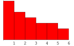
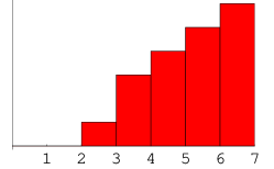
(a) $c_{1}(N_{S|B})>0$ ($A_{n},D_{n}$)		(b) $c_{1}(N_{S|B})<0$ ($A_{n},D_{n}$)

Figure 1: Extra tuning cost $-(\Delta L_{*})/(\Delta{\rm rank})$ decreases or increases for higher rank, depending on whether $c_{1}(N_{S|B_{3}})$ is positive or negative, as one goes down the $A_{n}$ or $D_{n}$ chain. $c_{1}(N_{S|B})$ is replaced by $K_{S}$ in the case of $E_{n}$ series.

When a divisor $c_{1}(N_{S|B_{3}})$ on $S$ is negative, in particular, it may happen sometimes that $\Delta L_{*}/\Delta{\rm rank}=0$ for a choice of 7-brane gauge group with a small rank; the rank of 7-brane gauge group can be large to some extent without losing the number of flux vacua. This is the phenomenon called non-Higgsable cluster [20, 28]. When either $\mathop{\rm SU}(3)_{C}$ or $\mathop{\rm SU}(2)_{L}$ or both are identified with 7-brane gauge groups in a non-Higgsable cluster [35], the tuning cost argument above is affected inevitably. In a family of fourfolds where the Mordell–Weil group is non-trivial everywhere on its complex structure parameter space [36], we cannot talk of relative statistical cost of requiring an extra U(1) symmetry; in such a case, we need to discuss relative tuning cost of U(1) through some transitions connecting such a family to another where the fourfolds have different topology, or to use the prefactor in (1) directly to estimate the number of flux vacua.

4 Distribution of Lagrangian Parameters

While the prefactor in the formula (1) can be used to estimate the number of flux vacua with a given set of algebraic and topological properties (i.e., symmetry, matter multiplicity etc.), the $(m,m)$-form $\rho_{I}$ in (1) can be used to “derive” distribution of Lagrangian parameters in such an ensemble of vacua. This is a source of rich information, as is evident already in its applications to Type IIB compactifications [37, 38]. In this section, we will discuss its F-theory applications in the context of particle physics.

It should be remembered, though, that the expression for $\rho_{I}$ was derived by assuming that the continuous approximation of the $K$-dimensional flux space is good, while the approximation is not good in the case of $K\gg L_{*}$. It may be that the distribution $\rho_{I}$ remains to have reasonable level of predictability, while the problem of bad approximation is mitigated, when the complex structure parameter space ${\cal M}_{*}$ is binned very coarsely, and $\rho_{I}$ is used only by being integrated over such a large bin. Justification is not given even to this hope, however. When one is interested in the choice of $(B_{3},[S])$ where $K\gg L_{*}$, one should keep this remark in mind.

4.1 Symmetry Breaking Scale of an Approximate U(1) Symmetry

In section 4.1, we work on an application of the distribution $\rho_{I}$ that extracts its potential power very well. Section 4.2 is devoted to a more problem-oriented application.

While it is not theoretically impossible to compute period integrals and evaluate $\rho_{I}$, it is not practical to do so, when there are O(1000) complex structure parameters. Fortunately, it is possible to learn essential features of the distribution $\rho_{I}$ without carrying out such computations, as experience in Type IIB applications indicates [37, 39]. First, the parameter space of complex structure ${\cal M}_{*}$ has a natural set of coordinates; in the case Calabi–Yau $n$-fold is given by a toric hypersurface, for example, we can use, for the coordinates of ${\cal M}_{*}$, various products of monomial coefficients that are invariant under rescaling, [40]. The distribution $\rho_{I}$ will show more or less uninteresting behaviour on these coordinates in ${\cal M}_{*}$, except at special loci in ${\cal M}_{*}$. $\rho_{I}$ exhibits singular behaviour in these coordinates, when the period integrals involve logarithm of those coordinates; only derivatives of logarithm introduce poles. Logarithm of such coordinates indicates that there is a non-trivial monodromy of cycles [39]. All these arguments above holds true for applications to Calabi–Yau fourfolds.

Consider a family of Calabi–Yau fourfolds $Y_{n=4}$ obtained as a hypersurface of an ambient space given by $WP_{[1:2:3]}$-fibration over some $B_{3}$;

$$X^{3}+Y^{2}+XYZA_{1}+X^{2}Z^{2}A_{2}+YZ^{3}A_{3}+XZ^{4}A_{4}+Z^{6}A_{6}=0,$$ (25)

with $A_{k}\in\Gamma(B_{n-1=3};{\cal O}_{B}(-kK_{B}))$. Let ${\cal M}_{*}$ be its parameter space of complex structure. Sitting within this family is a family of Calabi–Yau fourfolds with the ambient space replaced by ${\rm Bl}_{[1:0:0]}W\mathbb{P}_{[1:2:3]}$-fibration over $B_{3}$; the last term $Z^{6}A_{6}$ is simply dropped (followed by small resolution) to get to the sub-family given by (49), where there is a non-trivial section in $Y_{4}$, and hence a U(1) symmetry in the low-energy effective theory. Let ${\cal M}_{*}^{\mathop{\rm U}(1)}\subset{\cal M}_{*}$ be the locus of this sub-family. We study the behaviour of $\rho_{I}$ on ${\cal M}_{*}$ near the locus of this sub-family.

In the $A_{6}\longrightarrow 0$ limit, $Y_{4}$ has a curve of codimension-three conifold singularity, $X=Y=A_{3}=A_{4}=0$ [19]; this curve in $B_{3}$ is denoted by $\Sigma$. The conifold transition in such a limit was studied extensively in [41]. The genus of this curve is determined by

$$2g(\Sigma)-2=(-3K_{B})\cdot(-4K_{B})\cdot(-6K_{B})=72(c_{1}(TB_{3}))^{3}.$$ (26)

Incidentally, the parameter space ${\cal M}_{*}^{\mathop{\rm U}(1)}$ for this $A_{6}\longrightarrow 0$ limit is of complex codimension-$(-\Delta h^{3,1})$ in ${\cal M}_{*}$, where

$$(-\Delta h^{3,1})=h^{0}(B_{3};{\cal O}_{B}(-6K_{B}))-h^{0}(B_{3};{\cal O}_{B}(-3K_{B}))-h^{0}(B_{3};{\cal O}_{B}(-2K_{B}));$$ (27)

the first term is obviously the degree of freedom in $A_{6}$. The last two terms are there because only the $\epsilon_{1}$-term in the automorphism of the form

$$\delta Y=XZ\epsilon_{1}+Z^{3}\epsilon_{3},\qquad\delta X=Z^{2}\epsilon_{2},\qquad\epsilon_{k}\in\Gamma(B_{3};{\cal O}_{B}(-kK_{B}))$$ (28)

survives for $Y_{4}$ in the sub-family over ${\cal M}_{*}^{\mathop{\rm U}(1)}$. One can see that $(-\Delta h^{3,1})=g$, at least when $B_{3}$ is a Fano variety. Indeed, because the divisor $(-K_{B})$ is ample, Kodaira’s vanishing theorem implies that

$$h^{q}(B_{3};{\cal O}_{B}(-nK_{B}))=0\qquad\qquad{\rm for~{}}q>0,\quad n\geq 0.$$ (29)

Combining this theorem and the expression for $(-\Delta h^{3,1})$, we find that

$$(-\Delta h^{3,1})=36(c_{1}(TB_{3}))^{3}+1=g.$$ (30)

This agreement always holds at local level, but $(-\Delta h^{3,1})=g-\tilde{h}^{2,1}\leq g$ at global level [41]; the argument above shows that $\tilde{h}^{2,1}=0$ at least when $B_{3}$ is a Fano variety.

$6g-3$ topological four-cycles are identified in the local geometry of $Y_{4}$ [41], and all of them are lifted to topological cycles in $Y_{4}$, at least when $B_{3}$ is a Fano variety. Period integrals on these $6g-3$ four-cycles vanish when all the $g$ transverse coordinates of ${\cal M}_{*}^{\mathop{\rm U}(1)}\hookrightarrow{\cal M}_{*}$ are set to zero; see [41] and the appendix C. We found, in the appendix C.2, that there are at least $g$ independent generators of unipotent monodromy acting on these topological four-cycles, and the period integrals are of the form,

$$\Pi_{\widetilde{A}_{k}}\sim z_{k},\qquad\Pi_{\widetilde{C}^{k}}\sim c^{kl}z_{l}\ln(z^{\prime}s);$$ (31)

the $A_{6}\longrightarrow 0$ limit corresponds to $z_{1}=z_{2}=\cdots z_{g}=0$. It is then quite likely, as in [37, 39], that the $(m,m)$-form distribution $\rho_{I}$ on ${\cal M}_{*}$ has an asymptotic behaviour

$$\rho_{I}\approx\rho_{I}^{\mathop{\rm U}(1)}\wedge\rho_{I}^{\perp},\qquad\rho_{I}^{\perp}:=\prod_{k=1}^{g}\frac{dz_{k}\wedge d\bar{z}_{k}}{|z_{k}|^{2}(\ln(|z|^{2}))^{2}}\sim\prod_{k=1}^{g}d[{\rm arg}(z_{k})]\wedge\frac{d\ln(1/|z_{k}|^{2})}{[\ln(1/|z_{k}|^{2})]^{2}}$$ (32)

near ${\cal M}_{*}^{\mathop{\rm U}(1)}$. While derivation of the asymptotic form above is not as rigorous as it is desired to be, let us explore what this behaviour implies, if it is true.

The most important consequence is that the fraction of flux vacua with hierarchically small value of $\mathop{\rm U}(1)$ symmetry breaking parameter $|z_{k}|$ is not hierarchically small, but is only suppressed by some power of the logarithm of the hierarchy, $\ln(1/|z_{k}|^{2})$. That makes it much more natural to think of approximate U(1) symmetry in bottom-up model building. Secondly, though, it is likely that the U(1) symmetry is preserved approximately only if all the $|z_{k}|$’s are hierarchically small; that is, what really matters will be a fraction of flux vacua satisfying, say, $|z_{k}|^{2}<\delta$ for ${}^{\forall}k=1,\cdots,g$ for some small $\delta$. This then implies that only the fraction

$$\int_{{\cal M}_{*}^{\rm local};\leq\delta}\rho_{I}^{\perp}=\prod_{k}\left[\int_{\ln(1/\delta)}^{+\infty}\frac{d\ln(1/|z_{k}|^{2})}{[\ln(1/|z_{k}|^{2})}\right]=\frac{1}{[\ln(1/\delta)]^{g}}$$ (33)

of flux vacua in ${\cal M}_{*}$ has such an approximate U(1) symmetry. The value of $g(\Sigma)$ is often quite large; when $B_{3}=\mathbb{P}^{3}$, for example, $g=36\times 4^{3}+1$. Thus, the fraction of flux vacua decreases very quickly, when we require the approximate U(1) symmetry to be preserved for very hierarchically small $\delta$.

Let us take one more step and ask the following question. Although $\rho_{I}$ or (1) is presented in the form of a continuous distribution, it is originally a scatter plot on ${\cal M}_{*}$ of isolated flux vacua. What is the smallest value $\delta_{\rm min}$ of the approximately preserved U(1) symmetry in ${\cal M}_{*}\;\backslash\;{\cal M}_{*}^{\mathop{\rm U}(1)}$? This is a prototype of such questions as what the minimum symmetry breaking scale is for supersymmetry and flavour symmetry in string landscape.

A wild speculation will be to think as follows. When we set $\delta$ small enough, the fraction of flux vacua (33) becomes so small that it reaches the fraction of flux vacua on ${\cal M}_{*}^{\mathop{\rm U}(1)}$ among those on ${\cal M}_{*}$. The integral of $\rho_{I}^{\perp}$ over the normal coordinates of ${\cal M}_{*}^{\mathop{\rm U}(1)}\hookrightarrow{\cal M}_{*}$ in such a small region as $|z_{k}|^{2}<\delta$ may correspond to flux vacua that sit right on top of the ${\cal M}_{*}^{\mathop{\rm U}(1)}$ locus. This thought leads to a relation

$$\left[\frac{1}{\ln(1/\delta_{\rm min})}\right]^{g}=\exp\left[\frac{\ln(24)}{4}(\Delta h^{3,1})\right],$$ (34)

where (14)—valid for cases with $h^{3,1}\gg h^{1,1}$—was used in the right hand side. Geometry dependence through $g=-\Delta h^{3,1}$ drops out from this relation then, and we find that

$$\delta_{\rm min}\sim\exp\left[-e^{\frac{\ln(24)}{4}}\right].$$ (35)

This “prediction”, however, is not as powerful as it looks. We have to keep in mind the limited reliability in the value of “$\ln(24)/4$”, as remarked in footnote 12. It will not be still too bad to conclude that $\delta_{\rm min}$ will not be much smaller than

$$\exp[-e^{({\rm a~{}few})}]\approx\exp[-10]\approx 10^{-(3\mbox{-}4)},$$ (36)

provided all the speculative arguments leading to this conclusion are not wrong.

4.2 Statistical Cost of Yukawa Hierarchical Structure Problem

In section 4.2, we discuss the fraction of flux vacua that realise solutions to the hierarchical structure problem of Yukawa matrices. Each one of codimension-three singularity (matter-curve intersection) points in F-theory compactification for SU(5) unification gives rise to an approximately rank-1 Yukawa matrix, provided complex structure is generic [42, 43, 44, 45], but the up-type [resp. down-type and charged lepton] Yukawa matrix in the low-energy effective theory below the Kaluza–Klein scale receives contributions from all the “$E_{6}$”-type points [resp. $D_{6}$ type] on $S\subset B_{3}$. The number of “$E_{6}$”-type and $D_{6}$-type points are determined by topological intersection numbers, and are generically not equal to one [45, 46]. The approximately rank-1 nature of the Yukawa matrices at short distance in F-theory is therefore lost at energy scale below the Kaluza–Klein scale, at least in a generic flux vacuum. There have been proposed a few ideas, however, how to exploit the approximate rank-1 nature at short distance. We pick up two among them for the study in this section 4.2.

One of the two ideas is to tune parameters so that only a single “$E_{6}$”-type point contributes to the up-type Yukawa matrix in the effective theory below the Kaluza–Klein scale (and just one $D_{6}$-type point to the down-type Yukawa matrix); this idea was proposed originally in [43, 49] and the Yukawa matrices in this scenario have been studied carefully in [50, 44, 51]. In order to make sure that the low-energy Yukawa matrix receives contribution only from just one “$E_{6}$”-type point, it is safe to consider that splitting of matter curves is controlled by a U(1) symmetry [11, 18, 19].

It is true that, for the CKM mixing angles to be small, the single “$E_{6}$”-type point and the single $D_{6}$-type point should be at the same point in $S$, or at least be close enough [52]; this property does not follow from a U(1) symmetry (and matter curve factorisation). If one is happy to ignore this aspect in the mixing angle and to focus on the hierarchical structure of the Yukawa eigenvalues for now, then the study in section 3.1 as well as section 4.1 can be used to study statistical aspects of this idea of tuning. We will be brief in section 4.2.1 for this reason.

The other idea whose tuning we discuss in section 4.2.2 is a string-theory implementation of the idea of [54]. Sections of a line bundle on a torus $T^{2}$ (a term “magnetised torus” is sometimes used for this) is given by Theta functions, which become approximately Gaussian for large complex structure of $T^{2}$; the exponentially small tail of the Gaussian wavefunctions is used to create hierarchical structure among three copies of $(Q,\bar{U},\bar{E})={\bf 10}$, which leads to realistic mixing angles and hierarchy in Yukawa eigenvalues [53, 55]. See [56, 45] for more detailed account of the string implementation of this idea. In this idea, therefore, one assumes that the matter curve for $\mathop{\rm SU}(5)$-10 representation has a large complex structure parameter. We estimate how much fraction of flux vacua we lose by requiring this tuning in the complex structure parameter of the matter curve, by exploiting the “distribution” $\rho_{I}$.

4.2.1 Split Matter Curve under a U(1) Symmetry

Suppose that the matter curves $\Sigma_{({\bf 10})}$ and $\Sigma_{(\bar{\bf 5})}$ for the ${\bf 10}$ and $\bar{\bf 5}$ representations of Georgi–Glashow SU(5) unification are split into irreducible pieces, due to an extra unbroken U(1) symmetry originating from a non-trivial section. Let $\Sigma_{({\bf 10})}=\cup_{a}\Sigma_{({\bf 10});a}$ and $\Sigma_{(\bar{\bf 5})}=\cup_{b}\Sigma_{(\bar{\bf 5});b}$ be the irreducible decomposition protected by the U(1) symmetry. The idea of [43, 49] assumes, among other things, that there is a pair $\Sigma_{({\bf 10});a0}$ and $\Sigma_{(\bar{\bf 5});b0}$ such that they intersect transversely (i.e., “$E_{6}$”-type) just once in the SU(5) 7-brane locus $S$; the matter ${\bf 10}=(Q,\bar{U},\bar{E})$ are localised in $\Sigma_{({\bf 10});a0}$ and $H_{u}$ in $\Sigma_{(\bar{\bf 5});b0}$, respectively, so that the single transverse intersection point gives rise to the approximately rank-1 up-type Yukawa matrix at low-energy. It is an interesting question whether there are such Calabi–Yau fourfold geometries. The two constructions of fourfolds with a non-trivial Mordell–Weil group which we reviewed in the appendix A does not have enough freedom to accommodate such configuration of matter curves, but this is far from being a no-go. Given the variety of constructions for fourfolds with a non-trivial Mordell–Weil group [23], it may not be too bad to assume that there are constructions satisfying the assumption above. The rest of this section 4.2.1 is based on that assumption.

We have already estimated in section 3.1 the fraction of flux vacua that has an unbroken U(1) symmetry from a non-trivial Mordell–Weil group; factorisation of matter curves just follows as a consequence of the U(1) symmetry. Given the fact that the faction of such vacua depends on the choice of a construction of fourfolds with a non-trivial Mordell–Weil group, as well as on the choice of topology of $(B_{3},[S])$, we do not find it meaningful to estimate the cost at precision higher than in section 3.1. By using the results there, we conclude right away that the cost of extra U(1) symmetry to split the matter curves is something like

$$e^{-1000}\sim 10^{-{\cal O}(100)}\qquad\qquad{\rm for~{}}(B_{3},[S])=(\mathbb{P}^{1}\times\mathbb{P}^{2},H_{\mathbb{P}^{1}}).$$ (37)

The tuning cost estimated above should be compared against the naive estimate of the non-triviality of flavour structure of the Standard Model, first of all. Suppose that individual Yukawa eigenvalues are tuned to be small enough, one by one, by tuning the complex structure parameters by hand, and that these tunings for individual eigenvalues are can be carried out independently from each other. Then the total tuning cost of the hierarchical eigenvalues of the Standard Model by this naive individual tuning is estimated by

$$\left(\frac{\lambda_{c}}{\lambda_{t}}\frac{\lambda_{u}}{\lambda_{t}}\right)\left(\frac{\lambda_{e}}{\lambda_{\tau}}\frac{\lambda_{\mu}}{\lambda_{\tau}}\right)\approx\left(10^{-2}\cdot 10^{-4.5}\right)\times\left(10^{-1}\cdot 10^{-3.5}\right)=10^{-11}.$$ (38)

It is much easier, therefore, to obtain the semi-realistic hierarchical structure of Yukawa eigenvalues by just an accidental tuning, by chance of $10^{-11}$, than by matter-curve splitting under a Mordell–Weil U(1) symmetry, at least for choices of $(B_{3},[S])$ with $h^{3,1}\gg h^{1,1}$.

In fact, we may not have to require that the U(1) symmetry for matter curve splitting is exact. Higher precision is required for a U(1) symmetry in the application to the dimension-4 proton decay problem, but that is not the case in the application to flavour structure; the level of precision required for flavour physics is not more than $m_{e}/(174\;{\rm GeV})\sim 10^{-5.6}$. This motivates us to pay attention also to flux vacua with an approximate U(1) symmetry, where matter curves $\Sigma_{({\bf 10}}$ and $\Sigma_{(\bar{\bf 5})}$ are near the factorisation limit. Qualitative aspects of flux vacua distribution with an approximate U(1) symmetry in section 4.1 will remain the same, even after requiring an extra SU(5) symmetry on $S\subset B_{3}$, because the geometry of U(1) symmetry breaking (i.e., conifold transition) along a curve $s^{2}a_{3}=s^{3}a_{2}=0$ in $B_{3}$ in SU(5) models remains qualitatively the same as in the case without SU(5) unification, at least away from the GUT divisor $S\subset B_{3}$. An approximate U(1) symmetry is realised in much larger number of flux vacua than an exact U(1) symmetry is, and therefore the tuning problem for the hierarchical structure may be alleviated in this way.

It remains to be seen, however, to what extent the idea of [43, 49] works successfully even in the presence of a small symmetry breaking in the approximate U(1) symmetry. The question we asked at the end of section 4.1—the minimum symmetry breaking scale $\delta_{\rm min}$—may also become relevant in this context.

4.2.2 Gaussian Wavefunction due to Large Complex Structure

The second solution to the hierarchical structure problem of low-energy Yukawa matrices also requires tuning in one of the complex structure parameters. We use the distribution $\rho_{I}$ in (1) in order to estimate the fraction of flux vacua for this solution is.

As we have reminded ourselves at the beginning of section 4, the two important things in using $\rho_{I}$ are i) to identify the natural coordinates of the parameter space ${\cal M}_{*}$, and ii) to find out the locus of ${\cal M}_{*}$ where there is a unipotent monodromy on the four-cycles of $\hat{Y}_{4}$. Although we also need dictionary between the coordinates on ${\cal M}_{*}$ and parameters of the low-energy Lagrangian (Yukawa couplings in particular), this part has already been worked out in the literature at the level we need in the present context [14, 15, 42, 45].

The dictionary we use is the following. Let us use the base $B_{3}=\mathbb{P}^{1}\times\mathbb{P}^{2}$, and the SU(5) 7-brane locus $S={\rm pt}\times\mathbb{P}^{2}\subset B_{3}$ for concreteness. With generic choice of complex structure of a fourfold $\hat{Y}_{4}$ for SU(5) unification, the matter curve $\Sigma_{({\bf 10})}$ is an irreducible curve of genus 1, so that we can use the second solution. Let $\tau$ be the complex structure parameter of the genus one curve $\Sigma_{({\bf 10})}$. The $j$-invariant of an elliptic curve has an expansion

$$j\simeq e^{-2\pi i\tau}+744+{\cal O}(e^{2\pi i\tau})$$ (39)

which is convenient for large ${\rm Im}(\tau)$. Hierarchical Yukawa eigenvalues as well as small mixing angles in the CKM matrix follow, if ${\rm Im}(\tau)$ is parametrically large, or equivalently, the value of $|j(\Sigma_{({\bf 10})})|$ is exponentially large. This $j$-invariant of the genus one curve should be some modular function over the $m=h^{3,1}=2148$-dimensional space ${\cal M}_{*}$ of complex structure of this compactification for SU(5) unification.

The first task in this section 4.2.2 is to identify the natural coordinates on ${\cal M}_{*}$ and to find out how $j(\Sigma_{({\bf 10})})$ depends on these coordinates. The Calabi–Yau fourfold $\hat{Y}_{4}$ in question—for the choice of $(B_{3},[S])$—is given as a hypersurface of a toric variety:

$$y^{2}+x^{3}+ (a_{5|0}+sa_{5|1}+s^{2}a_{5|2})xy+(sa_{4|1}+s^{2}a_{4|2}+\cdots)x^{2}$$

$$+ (s^{2}a_{3|2}+s^{3}a_{3|3}+\cdots)y+(s^{3}a_{2|3}+\cdots)x+(s^{5}a_{0|5}+\cdots)=0,$$ (40)

where $s$ is the inhomogeneous coordinate of $\mathbb{P}^{1}$, and is regarded as the normal coordinate of $S\subset B_{3}$. We understand here that all the terms corresponding to interior lattice points of facets of the dual polytope are set to zero in this defining equation; the automorphism group action on the monomial coefficients is now gauge-fixed for the most part, and only the coordinate rescaling $(\mathbb{C}^{\times})^{4}$ acts on the coefficients. As a part of standard story in the toric hypersurface construction of Calabi–Yau manifolds, the complex structure parameter space ${\cal M}_{*}$ is given a natural set of coordinates; each one of them is in the form of

$$z_{a}:=\prod_{\tilde{\nu}_{\alpha}}(a_{\alpha})^{\tilde{\ell}^{a}_{\alpha}},$$ (41)

where $\alpha$ runs over the monomials in the defining equation, and $a$ labels linear relations $\sum_{\alpha}\tilde{\ell}^{a}_{\alpha}\tilde{\nu}_{\alpha}=0$ in the dual lattice $M$ of the toric data (e.g. [40]). In the case of $\hat{Y}_{4}$ we consider, there are 2148 such coordinates.

The matter curve $\Sigma_{({\bf 10})}$ is given by $a_{5|0}=0$, and $a_{5|0}$ is a cubic homogeneous function on $S\cong\mathbb{P}^{2}$:

$$a_{5|0}=a^{5|0}_{300}T^{3}+a^{5|0}_{210}T^{2}U+a^{5|0}_{201}T^{2}V+\cdots+a^{5|0}_{003}V^{3}.$$ (42)

None of the ten terms in this cubic form correspond to an interior point of a facet of the dual polytope, and hence we should retain all of them. Using the ten coefficients $a^{5|0}_{300},\cdots,a^{5|0}_{003}$, seven independent rescaling invariants (i.e., the coordinates of the form (41)) can be constructed. The $j$-invariant of $\Sigma_{({\bf 10})}$ should depend on the seven coordinates out of the 2148 coordinates of ${\cal M}_{*}$.

Before talking of how the $j$-invariant of a generic cubic curve of $\mathbb{P}^{2}$ depends on its monomial coefficients, let us have a look at the result for easier ones. When an elliptic curve is given in the Weierstrass form or Hesse form, the $j$-invariant is given in this way:

$$y^{2}=x^{3}+fx+g: \qquad j=4^{4}\times 27\frac{f^{3}}{4f^{3}+27g^{2}},$$ (43)

$$a_{1}X^{3}+a_{2}Y^{3}+a_{3}Z^{3}+a_{0}XYZ=0: \qquad j=-\frac{z(z-216)^{3}}{27(z+27)},\quad z:=\left(\frac{a_{0}^{3}}{a_{1}a_{2}a_{3}}\right).$$ (44)

The condition ${\rm Im}(\tau)\gg 1$ corresponds to the vanishing locus of the denominator, $4f^{3}+27g^{2}\simeq 0$ or $z+27\simeq 0$, or the discriminant locus, to put differently. When the defining equation is in the Jacobi form,

$$w^{2}=c_{0}u^{4}-c_{1}u^{3}+c_{2}u^{2}-c_{3}u+c_{4},$$ (45)

the discriminant locus is given by

$$6912c_{0}^{3}c_{4}^{3}-3456c_{0}^{2}c_{2}^{2}c_{4}^{2}+432c_{0}c_{2}^{4}c_{4}-5184c_{0}^{2}c_{1}c_{3}c_{4}^{2}$$

$$- 2160c_{0}c_{1}c_{2}^{2}c_{3}c_{4}-162c_{0}c_{1}^{2}c_{3}^{2}c_{4}+27c_{1}^{2}c_{2}^{2}c_{3}^{2}-108c_{1}^{3}c_{3}^{3}$$

$$- 729c_{1}^{4}c_{4}^{2}+3888c_{0}c_{1}^{2}c_{2}c_{4}^{2}-108c_{1}^{2}c_{2}^{3}c_{4}+486c_{1}^{3}c_{2}c_{3}c_{4}$$

$$- 729c_{0}^{2}c_{3}^{4}+3888c_{0}^{2}c_{2}c_{3}^{2}c_{4}-108c_{0}c_{2}^{3}c_{3}^{2}+486c_{0}c_{1}c_{2}c_{3}^{3}=0.$$ (46)

For the $j$-invariant of those curves to be exponentially large, which is what we want for phenomenology, then the discriminant needs to be exponentially small; that seems to be a general lesson from elliptic curves given by those different forms of defining equations.

The matter curve $\Sigma_{({\bf 10})}$ is given by a generic cubic (42) in $\mathbb{P}^{2}$, but this is not much different from all the elliptic curves above. Any generic cubic can be cast into the Jacobi form (45) (e.g., [57]; recent appearance in physics literature includes [58]). Using the discriminant locus of the Jacobi form (46), one can then detect the discriminant locus in the coefficients of the general cubic form, and hence in the complex structure parameter space ${\cal M}_{*}$ of F-theory compactification. This procedure is easier when such a point as $[T:U:V]=[0:0:1]$ is in the curve $a_{5|0}=0$ (i.e., $a^{5|0}_{003}=0$); the left-hand side of (46)—a homogeneous function of $c_{0,1,2,3,4}$ of degree 6—becomes a homogeneous function of $a^{5|0}_{***}$’s ($a^{5|0}_{003}=0$) of degree 12. The most general case, where $a^{5|0}_{003}$ does not necessarily vanish, can be reduced to the $a^{5|0}_{003}=0$ case above, by redefinition of the coordinates, $T\rightarrow T+solV$, $a^{5|0}_{300}sol^{3}+a^{5|0}_{201}sol^{2}+a^{5|0}_{102}sol+a^{5|0}_{003}=0$. It appears, then, that the expression (46) would involve a cubic root of a function of the coefficients $a^{5|0}_{***}$’s, but those terms cancel, and the expression of the discriminant turns into a form

$$\propto{\rm polynomial}_{1}\sqrt{{\rm polynomial}_{3}}+{\rm polynomial}_{2}.$$ (47)

The discriminant locus of the general cubic form should be the zero locus of an expression proportional to $({\rm polynomial}_{1})^{2}{\rm polynomial}_{3}-({\rm polynomial}_{2})^{2}$. This polynomial in the ten coefficients $a^{5|0}_{***}$ can be rewritten as a rational function of the seven coordinates $z_{a}$’s of ${\cal M}_{*}$ modulo an overall factor that is not relevant in the present context. Once again, this rational function of $z_{a}$’s needs to be exponentially small, in order for the solution to the hierarchical structure problem to work.

The complex structure parameter space ${\cal M}_{*}$ has a codimension-1 locus of ${\rm Im}(\tau)=\infty$, or equivalently $j(\Sigma_{({\bf 10})})=\infty$. Unless there is unipotent monodromy around this locus (an issue we come back to shortly), the distribution of $\rho_{I}$ will remain featureless around this locus, and the fraction of vacua for the phenomenological solution is estimated by how finely tuned the normal coordinate has to be for phenomenology. Hierarchically small Yukawa eigenvalues require that the value of the normal coordinate (the rational function in $z_{a}$’s) be hierarchically small. Because a single tuning of $1/j(\Sigma_{({\bf 10})})$ already does the job (including the CKM mixing angles), however, the total tuning cost in this solution will not be as severe as $10^{-11}$ (or $10^{-11}\times 10^{-4.5}$) estimate for the naive individual tunings in (38).

It is worth noting that the idea of [54] was to translate the hierarchically small values of Yukawa eigenvalues into a moderately large (but not hierarchically large) parameter in the exponent (like ${\rm Im}(\tau)$). In the F-theory implementation [55, 45] of this idea, however, the value of ${\rm Im}(\tau)$ is likely not to be the right measure of required fine-tuning, but the value of $1/j(\Sigma_{({\bf 10})})\sim e^{2\pi i\tau}$ is, in the statistics of F-theory flux vacua, according to the argument above.

Let us briefly have a look at whether the distribution $\rho_{I}$ on ${\cal M}_{*}$ has singularity at the $j(\Sigma_{({\bf 10})})=\infty$ locus; if it does, then the right measure of fine-tuning will not be $e^{2\pi i\tau}$ but $1/{\rm Im}(\tau)$. Certainly the ${\rm Im}(\tau)=i\infty$ point is the locus of unipotent monodromy of one-cycles on $\Sigma_{({\bf 10})}$. There may also be some unipotent monodromy among three-cycles in the matter surface for $\mathop{\rm SU}(5)$-${\bf 10}$ representation, because of the monodromy of one-cycles. The matter surface—a four-cycle—remains invariant in this limit, however. The author does not have a positive or negative evidence for non-trivial monodromy of four-cycles at the $j(\Sigma_{({\bf 10})})=\infty$ locus of the complex structure moduli space ${\cal M}_{*}$; positive evidence is necessary in order to avoid the conclusion in the previous paragraph.

Acknowledgements

The author thanks Andreas Braun, James Halverson, Bert Schellekens, Yuji Tachikawa, Tsutomu Yanagida and Timo Weigand for discussions and communications. He also owes a lot to the organisers and participants of workshops “Physics and Geometry of F-theory” at Max Planck Institute, Munich and “Stringphenomenology 2015” at IFT, Madrid. This work is supported in part by WPI Initiative and a Grant-in-Aid for Scientific Research on Innovative Areas 2303, MEXT, Japan.

Appendix A Fourfolds for $\mathop{\rm SU}(5)\times\mathop{\rm U}(1)$ Symmetry

This appendix is a brief summary note on Calabi–Yau fourfold geometry to be used for F-theory compactification when one wants to have $\mathop{\rm SU}(5)\times\mathop{\rm U}(1)$ symmetry in the effective theory below the Kaluza–Klein scale. There may be a few statements in the following that have not been written down in the literature, but those results can be derived by using procedure that has become almost standard these days. For this reason, only the results are stated, without detailed explanation.

In this article, we only consider elliptic fibration with a section for F-theory compactification; let $\hat{Y}_{n}$ be a non-singular Calabi–Yau $n$-fold, $\pi:\hat{Y}_{n}\longrightarrow B_{n-1}$ an elliptic fibration morphism, and we assume that there is a divisor $\sigma_{0}$ of $\hat{Y}_{n}$ which is one-to-one with the base $B_{n-1}$ under $\pi$, except in complex codimension-two loci in $B_{n-1}$. Low-energy effective theory has a U(1) symmetry, if the elliptic fibration $\pi:\hat{Y}_{n}\longrightarrow B_{n-1}$ has more sections than just a single section $\sigma_{0}$ [20].

We restrict our attention to cases where toric surfaces are used to construct the elliptic curve $E$ in the fibre. It is best to use a toric surface such as $WP_{[1:2:3]}$ and $F_{1}=dP_{1}$ (Hirzebruch surface), where the polytope $\widetilde{\Delta}_{F}\subset(\mathbb{Z}\oplus\mathbb{Z})\otimes\mathbb{R}=:N_{F}\otimes\mathbb{R}$ contains a vertex $\nu^{\prime}_{v}$ whose two neighbouring lattice points on $\widetilde{\Delta}_{F}$, denoted by $\nu^{\prime}_{a}$ and $\nu^{\prime}_{b}$, satisfy $\nu^{\prime}_{a}+\nu^{\prime}_{b}=\nu^{\prime}_{v}$ [60]; the divisor corresponding to $\nu^{\prime}_{v}$ then defines one point in $E$. In such toric surfaces as ${\rm Bl}_{[1:0:0]}WP_{[1:2:3]}$ and $F_{1}$ (whose toric data are shown in Table 1), there is one more independent divisor which can be chosen to be degree-1 on $E$;

divisor toric vectors in $N_{F}$ $D^{\prime}_{X}$ $\nu^{\prime}_{X}=(-1,0)$ $D^{\prime}_{Y}$ $\nu^{\prime}_{Y}=(0,-1)$ $D^{\prime}_{Z}$ $\nu^{\prime}_{Z}=(2,3)$ $D^{\prime}_{W}$ $\nu^{\prime}_{W}=(-1,-1)$	divisor toric vectors in $N_{F}$ $D^{\prime}_{0}$ $\nu^{\prime}_{0}=(0,1)$ $D^{\prime}_{\infty}$ $\nu^{\prime}_{\infty}=(0,-1)$ $D^{\prime}_{1}$ $\nu^{\prime}_{1}=(1,0)$ $D^{\prime}_{2}$ $\nu^{\prime}_{2}=(-1,1)$
(a) ${\rm Bl}_{[1:0:0]}WP_{[1:2:3]}$	(b) $F_{1}$

Table 1: Toric vectors in $N_{F}=\mathbb{Z}\oplus\mathbb{Z}$ for ${\rm Bl}_{[1:0:0]}WP_{[1:2:3]}$ (weighted projective space $WP^{2}_{[1:2:3]}$ blown up at one point) and a Hirzebruch surface $F_{1}=dP_{1}$. The two neighbouring lattice points of the polytope for $\nu^{\prime}_{Z}$ in (a) [resp. $\nu^{\prime}_{0}$ in (b)] are $(1,2)$ and $(1,1)$ [resp. $\nu^{\prime}_{1}$ and $\nu^{\prime}_{2}$], which sum up to be $\nu^{\prime}_{Z}$ [resp. $\nu^{\prime}_{0}$]; this means that $D^{\prime}_{Z}$ [resp. $D^{\prime}_{0}$] can be used as a section. Those two neighbouring points are both vertices of the polytope in (b), while they are not in (a); this makes it impossible to introduce the twisting by ${\cal O}_{B_{n-1}}(\kappa^{1,2})$ in the case (a) without introducing an unintended non-Abelian symmetry $\mathop{\rm SU}(3)\times\mathop{\rm SU}(2)$.

this divisor defines another point in $E$. When such a toric surface is fibred over some base $B_{n-1}$ to be an ambient space for $\hat{Y}_{n}$, those two points in $E$ become sections of the elliptic fibration. The rest of this note deals only with the two toric surfaces above. See [22] for other choices of toric surfaces to be fibred.

A.0.1 ${\rm Bl}_{[1:0:0]}WP_{[1:2:3]}$-fibred Ambient Space

A Calabi–Yau $n$-fold $Y_{n}$ is constructed as a hypersurface of an ambient space

$$\mathbb{P}_{\left\{\begin{array}[]{lccr}(-1&0&1&1)\\ (0&1&2&3)\end{array}\right\}}\left[{\cal O}_{B}\oplus K_{B}\oplus{\cal O}_{B}\oplus{\cal O}_{B}\right].$$ (48)

Here, the rank-4 fibre of the bundle over the base $B_{n-1}$ is made projective under the $\mathbb{C}^{\times}\times\mathbb{C}^{\times}$ action; one can choose two independent relations among the toric vectors in the form of $\sum_{i}\ell_{i}\nu^{\prime}_{i}=0\in N_{F}=\mathbb{Z}\oplus\mathbb{Z}$, such as $-\nu^{\prime}_{W}+\nu^{\prime}_{X}+\nu^{\prime}_{Y}=0$ and $\nu^{\prime}_{Z}+2\nu^{\prime}_{X}+3\nu^{\prime}_{Y}=0$, and define the corresponding $\mathbb{C}^{\times}$ actions as $(\lambda\in\mathbb{C}^{\times}):X_{i}\longrightarrow X_{i}\times\lambda^{\ell_{i}}$ for homogeneous coordinates $X_{i}$ corresponding to the toric divisors $D^{\prime}_{i}$. This ambient space is a ${\rm Bl}_{[1:0:0]}WP^{2}_{[1:2:3]}$-fibration over $B_{n-1}$.

A hypersurface $Y_{n}$ of this ambient space is given by an equation

$$X^{3}W^{2}+Y^{2}W+XYZWA_{1}+X^{2}Z^{2}WA_{2}+YZ^{3}A_{3}+XZ^{4}A_{4}=0,$$ (49)

where $A_{n}\in\Gamma(B_{n-1};{\cal O}_{B}(-nK_{B}))$ determines the complex structure of an elliptic fibred manifold $Y_{n}$. $X$, $Y$, $Z$ and $W$ are the homogeneous coordinates associated with divisors $D_{X}$, $D_{Y}$, $D_{Z}$ and $D_{W}$, respectively, which are the $D^{\prime}_{X}$, $D^{\prime}_{Y}$ $D^{\prime}_{Z}$ and $D^{\prime}_{W}$ divisors on the fibre, all over the base $B_{n-1}$. A section $D_{Z}|_{Y_{n}}$ is chosen as the zero section $\sigma_{0}$. Another section $\sigma_{1}=D_{W}|_{Y_{n}}=\{W=0\}|_{Y_{n}}$ does not intersect with the zero section $\sigma_{0}$. When the ambient space is blown down to the $WP_{[1:2:3]}$-fibred one, $D_{W}$ is mapped to $(x,y):=(XW/Z^{2},YW/Z^{3})=(0,0)$.

The $n$-fold $Y_{n}$ develops a complex codimension-two locus of $A_{4}$ singularity (when the fibre of the ambient space is blown down to $WP_{[1:2:3]}$), when we require

$$A_{n}=s^{n-1}a_{6-n},\qquad a_{n-1}\in\Gamma(B_{n-1};{\cal O}_{B}(-nK_{B}-(n-1)S))$$ (50)

for $n=1,\cdots,4$. $S$ is a divisor of $B_{n-1}$, and $s$ is a section of ${\cal O}_{B}(S)$ such that $S=\{s=0\}$. A non-singular $\hat{Y}_{n}$ is constructed by a standard process of $A_{4}$ singularity resolution, followed by small resolutions associated with loci of charged matter fields; Figure 2 (a) describes this process diagrammatically. Let this blow-up morphism be $\nu:\hat{Y}_{n}\longrightarrow Y_{n}$; we also use the same $\nu$ for the morphism between the corresponding ambient spaces.

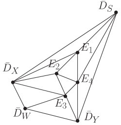
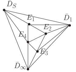
(a)		(b)

Figure 2: Blow-up procedure shown diagrammatically. Subdivision of a triangle using its centre of mass corresponds to a blow-up of the ambient space centred at a codimension-three locus, and a subdivision of an edge using its centre of mass to a blow-up of the ambient space centred at a codimension-two locus. These graphs can be seen as triangulation of cones, if the base $B_{n-1}$ is also toric, and the divisor $S$ a toric divisor, although we do not assume that $B_{n-1}$ is toric in this summary note. The diagram (a) is for the ${\rm Bl}_{[1:0:0]}WP^{2}_{[1:2:3]}$-fibred ambient space and (b) for the $F_{1}$-fibred ambient space. Note in (a) that the triangulation of $\bar{D}_{X}$-$E_{3}$-$\bar{D}_{Y}$-$\bar{D}_{W}$ resolves the conifold singularity associated with the $\mathop{\rm U}(1)$-charge $\pm 5$ matter field; the graph (b) is the same as the blow-up procedure in [61].

The zero section of $(\pi\cdot\nu):\hat{Y}_{n}\longrightarrow B_{n-1}$ is given by $\sigma_{0}:=\nu^{*}(D_{Z})|_{\hat{Y}_{n}}$; we will drop “$\nu^{*}$” or “$|_{\hat{Y}_{n}}$” in the following for simpler notations, however, unless subtleties are involved. Another section $\sigma_{1}\sim D_{W}$ for $\pi:Y_{n}\longrightarrow B_{n-1}$ defines a section in $\hat{Y}_{n}$ except subtleties in the fibre of $S\subset B_{n-1}$. When we set

$$\sigma^{\prime\prime}_{1}\sim\bar{D}_{W}-D_{Z}+K_{B}+(2E_{1}+4E_{2}+6E_{3}+3E_{4})/5,$$ (51)

where $\bar{D}_{W}$ is the proper transform of $D_{W}$ under $\nu:\hat{Y}_{n}\longrightarrow Y_{n}$, and $E_{1,2,3,4}$ the four exceptional divisors of $\nu:\hat{Y}_{n}\longrightarrow Y_{n}$, all of $\sigma^{\prime\prime}_{1}\cdot\sigma_{0}$ and $\sigma^{\prime\prime}_{1}\cdot E_{1,2,3,4}$ are mapped to the trivial divisor class in $B_{n-1}$ under $(\pi\cdot\nu)_{*}$. References for the statements up to this point include [62, 19, 63].

There are three distinct groups of $\mathop{\rm SU}(5)$-charged matter fields in this case [18], as summarised in Table 2.

bdle	repr.	curve def. eq.	curve div. class	vanishing cycle
${\bf 3}$	${\bf 10}_{-1}$	$a_{5}|_{S}=0$	$(-K_{B})|_{S}$	$(-E_{2}\cdot E_{4})|_{\hat{Y}_{n}}$
$\wedge^{2}{\bf 3}$	$\bar{\bf 5}_{-2}$	$(a_{4}a_{3}-a_{2}a_{5})|_{S}=0$	$(-3S-5K_{B})|_{S}$	$\left(-(\bar{D}_{Y}-K_{B}-E_{4})\cdot E_{3}\right)|_{\hat{Y}_{n}}$
$\wedge^{3}\bar{\bf 3}$	$\bar{\bf 5}_{+3}$	$a_{3}|_{S}=0$	$(-2S-3K_{B})|_{S}$	$(\bar{D}_{X}\cdot E_{3})|_{\hat{Y}_{n}}$

Table 2: Summary of geometry associated with the SU(5)-charged matter fields in the case of ${\rm Bl}_{[1:0:0]}WP^{2}_{[1:2:3]}$-fibred ambient space. The matter locus—codimension-1 in $S$—is given by the defining equation in the third column; this matter locus belongs to the divisor class on $S$ shown in the fourth column. The last column shows the corresponding class of vanishing cycle (complex codimension-two in $\hat{Y}_{n}$). The first column shows the representation of the $\mathop{\rm U}(3)$ structure group of the Higgs bundle on $S$.

The U(1)-charge of these $\mathop{\rm SU}(5)$-charged matter fields can be determined by using the topological class of $\sigma^{\prime\prime}_{1}$ in (51); the results—shown in Table 2—indicates that the U(1) symmetry generated by $\sigma^{\prime\prime}_{1}$ shows up as the U(1) part of the $\mathop{\rm U}(3)\subset E_{7}$ structure group of the Higgs bundle in the field theory local model (Katz–Vafa type field theory) on $S\times\mathbb{R}^{3,1}$ (cf [18, 19]). The 6D anomaly cancellation condition indicates that an SU(5)-neutral hypermultiplet with U(1)-charge $\pm 5$ is localised in the fibre of a codimension-two $a_{2}=a_{3}=0$ locus in $B_{n-1}$, and that they are all the matter fields charged under the $\mathop{\rm SU}(5)\times\mathop{\rm U}(1)$ symmetry (see [19, 64]).

This construction can be used for spontaneous R-parity violation. The hierarchical structure problem of Yukawa eigenvalues, however, cannot be solved by using this construction (without further symmetry or tuning of parameters), because all the “$E_{6}$”-type points on $S$ contribute to the up-type Yukawa matrix in the low-energy effective theory. See Figure 3 (a) for the configuration of matter curves.

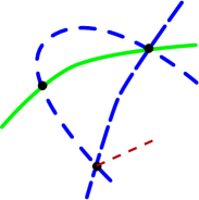
(a)		(b)

Figure 3: (colour online) Configuration of matter curves and interaction points on the SU(5) 7-brane $S$ shown schematically. The picture (a) is for the case of ${\rm Bl}_{[1:0:0]}WP^{2}_{[1:2:3]}$-fibred ambient space, and (b) for the case of $F_{1}$-fibred ambient space with the no.2 choice of the order of vanishing. Solid curve (green) is the matter curve for $\mathop{\rm SU}(5)$-10 representation in both (a) and (b). In the picture (a), the long dashed and dashed curves (both blue) are the matter curves for $\bar{\bf 5}_{3}$ and $\bar{\bf 5}_{-2}$, respectively. The dotted curve (red) is where SU(5)-neutral U(1)-charged fields are localised in $B_{3}$, “projected” on to $S$. In the picture (b), the long dashed, dashed, dotted and dash-dotted curves (all in blue) are the matter curves for $\bar{\bf 5}_{0}$, $\bar{\bf 5}_{-1}$, $\bar{\bf 5}_{1}$ and $\bar{\bf 5}_{2}$ representations, respectively. The “$E_{6}$”-type point for up-type Yukawa is indicated by a square (orange), while the point with $F_{1}$-fibre by a large circle (red).

A.0.2 $F_{1}$-fibred Ambient Space

$F_{1}=dP_{1}$ can be used as fibre of the ambient space, instead of ${\rm Bl}_{[1:0:0]}WP^{2}_{[1:2:3]}$, in constructing a Calabi–Yau $n$-fold with a non-trivial Mordell–Weil group. We then use an ambient space

$$\mathbb{P}_{\left\{\begin{array}[]{lccr}(1&1&0&0)\\ (0&1&1&1)\end{array}\right\}}\left[K_{B}\oplus{\cal O}_{B}\oplus{\cal O}_{B}(\kappa^{1})\oplus{\cal O}_{B}(\kappa^{2})\right],$$ (52)

where the fibre can be twisted by introducing two divisors $\kappa^{1}$ and $\kappa^{2}$ of the base $B_{n-1}$ [65]. The fibre is $F_{1}$; the four line bundles above correspond to the toric vectors $\nu^{\prime}_{0}$, $\nu^{\prime}_{\infty}$, $\nu^{\prime}_{1}$ and $\nu^{\prime}_{2}$ in Table 1 (b), respectively. The zero locus of the line bundles are the divisors denoted by $D_{0,\infty,1,2}$, and the corresponding homogeneous coordinates are denoted by $X_{0,\infty,1,2}$. There are linear equivalence relations

$$D_{1}-\kappa^{1}\sim D_{2}-\kappa^{2},\qquad D_{\infty}\sim D_{0}-K_{B}+D_{2}-\kappa^{2}.$$ (53)

An elliptic fibred Calabi–Yau $n$-fold $Y_{n}$ is given as a hypersurface of this ambient space by

$$X_{\infty}^{2}(A_{0,1}X_{1}+A_{1,0}X_{2})+X_{\infty}X_{0}(B_{-1,1}X_{1}^{2}+B_{0,0}X_{1}X_{2}+B_{1,-1}X_{2}^{2})$$

$$+X_{0}^{2}(C_{-2,1}X_{1}^{3}+C_{-1,0}X_{1}^{2}X_{2}+C_{0,-1}X_{1}X_{2}^{2}+C_{1,-2}X_{2}^{3})=0.$$ (54)

Complex structure of $Y_{n}$ is encoded in the choice of

$$A_{n_{1},n_{2}} \in\Gamma(B_{n-1};{\cal O}(n_{1}\kappa^{1}+n_{2}\kappa^{2})),$$

$$B_{n_{1},n_{2}} \in\Gamma(B_{n-1};{\cal O}(n_{1}\kappa^{1}+n_{2}\kappa^{2}-K_{B})),$$ (55)

$$C_{n_{1},n_{2}} \in\Gamma(B_{n-1};{\cal O}(n_{1}\kappa^{1}+n_{2}\kappa^{2}-2K_{B})).$$

We take $D_{0}$ ($X_{0}=0$ locus) as the zero section $\sigma_{0}$ of the elliptic fibration $\pi_{Y}:Y_{n}\longrightarrow B_{n-1}$. There is also a section corresponding to the degree-1 divisor $(D^{\prime}_{1}-D^{\prime}_{0})|_{E}$ of the fibre, which is denote by $\sigma_{1}$. It is geometrically given by

$$[X_{\infty}(B_{-1,1}X_{1}^{2}+\cdots+B_{1,-1}X_{2}^{2})+X_{0}(C_{-2,1}X_{1}^{3}+\cdots+C_{1,-2}X_{2}^{3})=0]-2[X_{\infty}=0],$$ (56)

and belongs to the divisor class $(D_{1}-D_{0}+\kappa^{2})$. Since

$$\pi_{Y*}(\sigma_{1}\cdot\sigma_{0})=[B_{sym}=0],$$ (57)

$$B_{sym}:=B_{1,-1}A_{0,1}^{2}-B_{0,0}A_{0,1}A_{1,0}+B_{-1,1}A_{1,0}^{2}\in\Gamma\left(B_{n-1};{\cal O}(\kappa^{1}+\kappa^{2}-K_{B})\right),$$ (58)

we take

$$\sigma^{\prime\prime}_{1}:=\sigma_{1}-[B_{sym}=0]-\sigma_{0}+K_{B}\sim(D_{1}-\kappa^{1}-2D_{0}+2K_{B})$$ (59)

as the generator of a U(1) symmetry in the low-energy effective theory.

The charge-$\pm 2$ matter fields under this U(1) symmetry are localised in the codimension-two locus of $B_{n-1}$ given by

$$B_{sym} =C_{sym}=0,$$ (60)

$$C_{sym} :=C_{1,-2}A_{0,1}^{3}-C_{0,-1}A_{0,1}^{2}A_{1,0}+C_{-1,0}A_{0,1}A_{1,0}^{2}-C_{-2,1}A_{1,0}^{3}\in\Gamma\left(B_{n-1};{\cal O}(\kappa^{1}+\kappa^{2}-2K_{B})\right).$$

Matter fields with charge $\pm 1$ are localised in a class $4(\kappa^{1}+\kappa^{2}-2K_{B})\cdot(-\kappa^{1}-\kappa^{2}-2K_{B})$. All that has been stated so far is the same as (or obvious generalisation of) [63, 21].

Let us consider a case where an $n$-fold $Y_{n}$ develops $A_{4}$ singularity at the $X_{\infty}=X_{1}=0$ point in the $F_{1}$ fibre over a divisor $S\subset B_{n-1}$, so that there is a stack of 7-branes for an SU(5) gauge theory along $S\subset B_{n-1}$. The sections $A_{n_{1},n_{2}}$, $B_{n_{1},n_{2}}$ and $C_{n_{1},n_{2}}$’s defining the complex structure of the $n$-fold $Y_{n}$ need to have certain order of vanishing along the divisor $S\subset B_{n-1}$ then. There are a couple of different choices, as shown in Table 3, at least in a study of local geometry.

choice	$A_{0,1}$	$A_{1,0}$	$B_{-1,1}$	$B_{0,0}$	$B_{1,-1}$	$C_{-2,1}$	$C_{-1,0}$	$C_{0,-1}$	$C_{1,-2}$
no.1	0	0	0	0	1	2	3	4	5
no.2	0	0	0	0	2	0	1	3	5
no.3	0	1	0	0	3	0	0	2	5
no.4	0	3	0	0	4	0	0	1	5

Table 3: The order of vanishing required for $A_{4}$ singularity.

The no.3 choice of the order of vanishing, however, may have a problem, when a global geometry is studied; at least in a few examples using compact toric ambient spaces, we found that the singular fibre over $S$ in a resolved $n$-fold $\hat{Y}_{n}$ becomes $I_{6}$ type of Kodaira classification unintentionally. The rest of this summary note focuses on the no.2 choice of the order of vanishing. It is not clear whether the choice of toric vectors in section 3 of [21] corresponds to any one of the order of vanishing in Table 3.

Under the no.2 choice of the order of vanishing, singular $Y_{n}$ can be made non-singular (denoted by $\hat{Y}_{n}$) by successive blow-ups of the ambient space; the same blow-up procedure as in [66], shown in Figure 3 (b), does the job in this case. The proper transforms of the divisor $D_{1}$, $D_{\infty}$ and $D_{S}=\pi_{Y}^{*}(S)$ are denoted by $\bar{D}_{1}$, $\bar{D}_{\infty}$ and $\bar{D}_{S}$, respectively.

$$D_{S}=\bar{D}_{S}+E_{1}+E_{2}+E_{3}+E_{4},\quad D_{1}=\bar{D}_{1}+E_{1}+2E_{2}+2E_{3}+E_{4},\quad D_{\infty}=\bar{D}_{\infty}+E_{1}+2E_{2}+3E_{3}+2E_{4}.$$

When we choose

$$\sigma^{\prime\prime}_{1}\sim(D_{2}-\kappa^{2}-2D_{0}+2K_{B})$$ (61)

as a U(1) generator, the conditions $(\pi_{Y}\cdot\nu)_{*}(\sigma_{0}\cdot\sigma^{\prime\prime}_{1})=(\pi_{Y}\cdot\nu)_{*}(E_{1,2,3,4}\cdot\sigma^{\prime\prime}_{1})=0\in{\rm Pic}(B_{n-1})$ are satisfied.

SU(5)-charged matter fields are localised in five distinct codimension-1 loci in $S$, as summarised in Table 4.

	matter curve def. eq. ($|_{S}=0$)	curve divisor class ($|_{S}$)	vanishing cycle ($|_{\hat{Y}_{n}}$)
${\bf 10}_{0}$	$B_{0,0}$	$-K_{B}$	$-E_{2}\cdot E_{4}$
$\bar{\bf 5}_{0}$	$(c_{1,-2|5}B_{0,0}^{2}-c_{0,-1|3}B_{0,0}b_{1,-1|2}+c_{-1,0|1}b_{1,-1|2}^{2})$	$\kappa^{1}-2\kappa^{2}-4K_{B}-5S$	$E_{3}\cdot(\bar{D}_{1}-E_{2}-K_{B})$
$\bar{\bf 5}_{-1}$	$A_{0,1}B_{0,0}^{2}-A_{1,0}B_{-1,1}B_{0,0}+C_{-2,1}A_{1,0}^{2}$	$\kappa^{2}-2K_{B}$	$-\bar{D}_{S}\cdot(D_{0}-E_{1}-K_{B})$
$\bar{\bf 5}_{1}$	$C_{-2,1}$	$-2\kappa^{1}+\kappa^{2}-2K_{B}$	$\bar{D}_{S}\cdot\bar{D}_{\infty}$
$\bar{\bf 5}_{2}$	$A_{1,0}$	$\kappa^{1}$	$\bar{D}_{S}\cdot(\kappa^{1}-\bar{D}_{1})$

Table 4: Summary of geometry associated with SU(5)-charged matter fields in the case of $F_{1}$-fibred ambient space, and the no.2 choice of the order of vanishing. See caption of Table 2.

There, we used the following notations, as in [67, 49]:

$$B_{1,-1}=:sb_{1,-1|1},\quad C_{-1,0}=:sc_{-1,0|1},\quad C_{0,-1}=:s^{3}c_{0,-1|3},\quad C_{1,-2}=:s^{5}c_{1,-2|5}.$$ (62)

The divisor classes of $\bar{\bf 5}$-representation matter fields sum up to be $(-8K_{B}-5S)|_{S}$, which is vital to the 6D box anomaly cancellation. There are also SU(5)-neutral, but U(1)-charged matter fields. Their location—codimension-two in $B_{n-1}$—is inferred by using the 6D anomaly cancellation conditions; we are led to the following solution:

$${\rm charge}~{}\pm 2 (\kappa^{1}+\kappa^{2}-K_{B})\cdot(\kappa^{1}+\kappa^{2}-2K_{B})-5S\cdot\kappa^{1}\subset B_{n-1},$$ (63)

$${\rm charge}~{}\pm 1 16K_{B}^{2}-4(\kappa^{1}+\kappa^{2})^{2}-10S\cdot(-\kappa^{1}+\kappa^{2}-2K_{B})\subset B_{n-1}.$$ (64)

A part of the $B_{sym}=C_{sym}=0$ locus for the charge-$\pm 2$ fields—$5S\cdot\kappa^{1}$—has been subtracted, which is reasonable because the $B_{sym}=C_{sym}=0$ conditions are satisfied automatically at $A_{1,0}=s=0$.

When F-theory is compactified to 3+1-dimensions in this way, by using a Calabi–Yau fourfold $\hat{Y}_{n=4}$, geometric configuration of the matter curves on $S$ is schematically like Figure 3 (b). Most of the intersection points of the matter curves in $S$ are one of the “$E_{6}$”-type, $D_{6}$ type and $A_{6}$-type, but none of those local descriptions apply to the intersection points where matter curves for ${\bf 10}_{0}$, $\bar{\bf 5}_{2}$ and $\bar{\bf 5}_{-1}$-representations meet. The fibre of $(\pi_{Y}\cdot\nu):\hat{Y}_{4}\longrightarrow B_{3}$ is a surface $F_{1}$ at such points in $B_{3}$. Tensionless strings may show up in the effective theory on 3+1-dimensions in this case [24]. For phenomenological purposes, it is thus safe to restrict our attention to cases where the divisor class $\kappa^{1}|_{S}$ is trivial (so that $A_{1,0}|_{S}$ remains non-zero on $S$).

This $\kappa^{1}|_{S}=0$ condition implies, first of all, that the $\bar{\bf 5}_{2}$–${\bf 5}_{-2}$ matter fields do not appear in the low-energy spectrum. When this set-up with a U(1) symmetry is used for spontaneous R-parity violation scenario, matter identification should be the following. First, the up-type Higgs needs to be identified with the doublet part of ${\bf 5}_{0}$ so that the up-type Yukawa couplings are generated. Secondly, for the charged lepton Yukawa couplings to be generated, $L$ and $H_{d}$ need to originate from $\bar{\bf 5}_{1}$ and $\bar{\bf 5}_{-1}$ or vice versa. $\bar{D}$’s of the supersymmetric Standard Models need to be on the same matter curve as $L$’s in order for the down-type Yukawa couplings to be generated.

The $\kappa^{1}|_{S}=0$ condition also implies that the splitting of the matter curve of $\bar{\bf 5}$ representation in this set-up cannot be used for the hierarchical structure problem of the up-type Yukawa matrix. In the absence of the matter curve of $\bar{\bf 5}_{2}$ matter field and of the interaction points indicated by a large circle (red) in Figure 3 (b), all the “$E_{6}$” type points arise in the form of ${\bf 10}_{0}$–${\bf 10}_{0}$–$\bar{\bf 5}_{0}$ interaction points at $c_{-1,0|1}=B_{0,0}=0$. Therefore, the result of [45, 46] that the number of “$E_{6}$”-type points is even still holds true.

Appendix B SU(6) 7-brane for Up-type Yukawa Coupling

Reference [9] introduced a class of F-theory compactification with a stack of SU(6) 7-branes at the divisor $S$ in the base $B_{n-1}$, which accommodates SU(5) unification and generates its up-type Yukawa couplings. Some details of the construction of this class of compactification were missing in [9], however. Thanks to the development in the study of F-theory since then, we can fill the missing details now.

Let us first note that the class of F-theory compactification with an SU(6) 7-brane locus above is somewhat different from general F-theory compactification characterised by the Tate condition for the $I_{6}$-type singular fibre. To see this, remember that the Tate condition for the $I_{6}$-type singular fibre in a non-singular elliptic fibration $\pi:\hat{Y}_{n}\longrightarrow B_{n-1}$ corresponds to the following set of the order of vanishing of the coefficients in the generalised Weierstrass form [67]:

$$0 = y^{2}+x^{3}+A_{1}xy+A_{2}x^{2}+A_{3}y+A_{4}x+A_{6},$$ (66)

$$A_{1}\sim s^{0},\quad A_{2}\sim s^{1},\quad A_{3}\sim s^{3},\quad A_{4}\sim s^{3},\quad A_{6}\sim s^{6};$$

here, $s\in\Gamma(B;{\cal O}_{B}(S))$, and the $\{s=0\}$ locus corresponds to the divisor $S$. It is thus convenient to write the Weierstrass equation in the following form:

$$y^{2}+x^{3}+a_{5}xy+a_{4}sx^{2}+a_{3}s^{3}y+a_{2}s^{3}x+a_{0}s^{6}=0.$$ (67)

where $a_{0,2,3,4,5}$ are holomorphic sections of appropriate line bundles on $B_{n-1}$.

When we consider F-theory compactification of this type to 3+1-dimensions, using a Calabi–Yau fourfold, straightforward analysis reveals that the matter curves in $S$ are given by

$$\Sigma_{(\wedge^{2}{\bf 6})}:\quad a_{5}|_{S}=0,\qquad\Sigma_{({\bf 6})}:\quad(a_{2}^{2}-a_{2}a_{5}a_{3}+a_{0}a_{5}^{2})|_{S}=0;$$ (68)

Katz–Vafa type field theory for these matter fields are SO(12) ($D_{6}$) and SU(7) ($A_{6}$) gauge theories, respectively. These two matter curves intersect at points $a_{5}|_{S}=a_{2}|_{S}=0$; physics around these points (including Yukawa couplings) is captured by a field theory with SO(14) ($D_{7}$) gauge group. We cannot expect an up-type Yukawa coupling of the form $\Delta W\sim{\bf 10}^{\cdot\cdot}{\bf 10}^{\cdot\cdot}{\bf 5}^{\cdot}\epsilon_{\cdot\cdot\cdot\cdot\cdot}$ in such a class of F-theory compactification [9, 68].

An idea of Ref. [9] is to use Heterotic compactification, and to translate and generalise it in the language of F-theory compactification. To be more explicit, imagine a Heterotic string compactification on an elliptic fibred Calabi–Yau threefold $(Z,S,\pi)$, where $\pi:Z\longrightarrow S$, with a vector bundle $V_{3}\oplus V_{2}$ whose structure group is $\mathop{\rm SU}(3)\times\mathop{\rm SU}(2)\subset E_{8}$. $V_{3}$ and $V_{2}$ are given by Fourier–Mukai transform of spectral data $(C_{3},{\cal N}_{3})$ and $(C_{2},{\cal N}_{2})$, where $C_{3}$ and $C_{2}$ are divisors of $Z$ that are 3-fold and 2-fold covering over $S$, respectively, and ${\cal N}_{3}$ and ${\cal N}_{2}$ are line bundles on $C_{3}$ and $C_{2}$, respectively. For generic complex structure of $Z$, the spectral surfaces $C_{3}$ and $C_{2}$ are given by

$$c_{0}+c_{2}x+c_{3}y=0,\qquad d_{0}+d_{2}x=0,$$ (69)

respectively, where

$$c_{k}\in\Gamma(S;{\cal O}_{S}(kK_{S}+\eta_{3})),\qquad d_{k}\in\Gamma(S;{\cal O}_{S}(kK_{S}+\eta_{2}))$$ (70)

for some divisors $\eta_{2,3}$ of $S$. The F-theory dual of this compactification should be given by $(Y_{4},B_{3})$, where the base threefold $B_{3}=\mathbb{P}\left[{\cal O}_{S}(6K_{S}+\eta_{3}+\eta_{2})\oplus{\cal O}_{S}\right]$ is a $\mathbb{P}^{1}$-fibration over $S$, and the elliptic fibre of $\pi:Y_{4}\longrightarrow B_{3}$ is given by [69, 14, 70, 42]

$$y^{2}=x^{3}+f_{0}xs^{4}+g_{0}s^{6}+(c_{0}s^{3}+c_{2}sx+c_{3}y)(d_{0}s^{2}+d_{2}x),$$ (71)

where $s$ is an inhomogeneous coordinate of the $\mathbb{P}^{1}$-fibre in $B_{3}\longrightarrow S$. Now, we generalise it to general $B_{3}$ and its effective divisor $S$, and define $\pi:Y_{4}\longrightarrow B_{3}$ by the same equation as above; the coefficients $f_{0}$, $g_{0}$, $c_{k}$’s and $d_{k}$’s, however, are promoted to holomorphic sections on $B_{3}$ as follows:

$$c_{k}\in\Gamma(B_{3};{\cal O}_{B}((k-4)K_{B}+a+(k-3)S)), f_{0}\in\Gamma(B_{3};{\cal O}_{B}(-4K_{B}-4S),$$ (72)

$$d_{k}\in\Gamma(B_{3};{\cal O}_{B}(-a+(k-2)(K_{B}+S))), g_{0}\in\Gamma(B_{3};{\cal O}_{B}(-6K_{B}-6S),$$ (73)

where $a$ is some divisor on $B_{3}$; this is a generalisation, in that the translation from Heterotic string compactification is reproduced by setting $(2K_{S}+\eta_{2})=-a|_{S}$ and $(6K_{S}+\eta_{2}+\eta_{3})=S|_{S}=c_{1}(N_{S|B_{3}})$.

One can read out from the discriminant and singularity of this generalised Weierstrass form that there are three distinct matter curves,

$$\Sigma_{(\wedge^{3}{\bf 6})}: d_{2}|_{S}=0,$$ (74)

$$\Sigma_{(\wedge^{2}{\bf 6})}: c_{3}|_{S}=0,$$ (75)

$$\Sigma_{({\bf 6})}: (c_{3}^{2}d_{0}^{3}+c_{2}^{2}d_{0}^{2}d_{2}-2c_{0}c_{2}d_{0}d_{2}^{2}+c_{0}^{2}d_{2}^{3}+c_{3}^{2}d_{0}d_{2}^{2}f_{0}-c_{3}^{2}d_{2}^{3}g_{0})|_{S}=0.$$ (76)

Those three curves intersect at $c_{3}|_{S}=d_{2}|_{S}=0$ points in $S$. We can choose the gauge group of the Katz–Vafa type field theory (field theory local model) around these matter curves to be $E_{6}$, $D_{6}$, $A_{6}$; physics around a $c_{3}|_{S}=d_{2}|_{S}=0$ point is described by an $E_{7}$ gauge theory; a non-trivial Higgs bundle background with the structure group $\mathop{\rm SU}(2)\times\mathop{\rm U}(1)\subset E_{7}$ breaks the $E_{7}$ symmetry down to SU(6); Yukawa coupling $\Delta W={\bf 6}\cdot\wedge^{2}{\bf 6}\cdot\wedge^{3}{\bf 6}$ is generated at each one of those $c_{3}|_{S}=d_{2}|_{S}=0$ points.

Such an SU(6) 7-brane in F-theory can be used for SU(5) unification by turning on a line bundle on $S$, so that the symmetry is reduced to SU(5); further breaking to the Standard Model gauge group is not impossible, although we stay away from such details. There are two possible particle identifications. The first possibility is to identify SU(5)-${\bf 10}$ matter fields with the $\wedge^{3}{\bf 6}$ representation of SU(6), and $H({\bf 5})$ within ${\bf adj}.$ of SU(6) [9]; the other possibility is to find the ${\bf 10}$ matter field in $\wedge^{2}{\bf 6}$ of SU(6), when the $H({\bf 5})$ field also has to come from the same $\wedge^{2}{\bf 6}$ representation of SU(6); the latter possibility was overlooked in [9]. In any one of those two possibilities, Yukawa couplings are generated along the entire matter curve ($\Sigma_{(\wedge^{3}{\bf 6})}$ or $\Sigma_{(\wedge^{2}{\bf 6})}$), not only at isolated points in the 7-brane $S$ (cf [15]). This makes it impossible to exploit the approximately codimension-1 nature of Yukawa matrices from isolated Yukawa points [42, 43, 44]. The idea of [55] (or something similar to the one in [45]) may still be implemented in the latter identification with a tuning $j(\Sigma_{(\wedge^{2}{\bf 6})})\gg 1$, it is desirable to have a separate study.

Before closing this section, we compute $h^{3,1}$ for Calabi–Yau fourfolds with such an SU(6) unification. We choose $(B_{3},[S])$ to be $B_{3}=\mathbb{P}^{1}\times\mathbb{P}^{2}$ and $[S]={\rm pt}\times\mathbb{P}^{2}$, so the result can be compared with $h^{3,1}$ for other classes of compactifications with a rank-5 symmetry (SO(10) and $\mathop{\rm SU}(5)\times\mathop{\rm U}(1)$) in the main text. The choice of $(B_{3},[S])$ above introduces a constraint $(3K_{S}+\eta_{2})+(3K_{S}+\eta_{3})=0$.

$(3K_{\mathbb{P}^{2}}+\eta_{2})$	$-2$	$-1$	0	1	2
$(3K_{\mathbb{P}^{2}}+\eta_{3})$	2	1	0	$-1$	$-2$
$h^{3,1}$	1918	1909	1905	1906	1912

Table 5: $h^{3,1}$ of Calabi–Yau fourfolds for SU(6) unification, provided $B_{3}=\mathbb{P}^{1}\times\mathbb{P}^{2}$ and $[S]={\rm pt}\times\mathbb{P}^{2}$.

See Table 5 for the results.

Appendix C Monodromy around the U(1)-enhancement Limit

C.1 $6g-3$ Topological Four-cycles

This appendix C begins with a brief review. We came to be interested in section 4.1 in a compact Calabi–Yau fourfold $Y_{4}$ with its complex structure parameter in ${\cal M}_{*}$ close to the ${\cal M}_{*}^{\mathop{\rm U}(1)}$ locus; $Y_{4}$ contains a local geometry of deformed conifold along a curve $\Sigma$, and this local geometry of $Y_{4}$ is modelled by a geometry $Y_{\rm local}$, which is explained shortly. Four-cycles in $Y_{\rm local}$ as well as their lift to the global geometry $Y_{4}$ was studied in [41]; results of [41] that we need in section 4.1 are reviewed here. The review is followed by analysis of monodromy of those cycles and period integrals.

The local geometry model $Y_{\rm local}$, which is denoted by $\widetilde{X}^{\flat}$ in [41], is realised as a hypersurface of the total space of a rank-4 vector bundle over a Riemann surface $\Sigma$,

$${\cal L}^{\otimes 3}\oplus{\cal L}^{\otimes 3}\oplus{\cal L}^{\otimes 2}\oplus{\cal L}^{\otimes 4}\longrightarrow\Sigma,$$ (77)

where the Riemann surface $\Sigma$ satisfies $6|(2g(\Sigma)-2)$, and ${\cal L}^{\otimes 6}=K_{\Sigma}$. The defining equation of $Y_{\rm local}$ in this ambient space is

$$YA_{3}=XA_{4}+A_{6};$$ (78)

$Y$, $A_{3}$, $X$ and $A_{4}$ are the coordinates of the rank-4 fibre of the bundle in (77), and

$$A_{6}\in\Gamma(\Sigma;K_{\Sigma})\cong\mathbb{C}^{g}=:{\cal M}_{*}^{\rm local}$$ (79)

governs the complex structure of this local geometry; this $A_{6}\in\Gamma(\Sigma;K_{\Sigma})$ descends from $A_{6}\in\Gamma(B_{3};{\cal O}_{B}(-6K_{B}))$ on the compact set-up by simple restriction on $\Sigma\subset B_{3}$. ${\cal L}^{\otimes 6}:={\cal O}_{\Sigma}(-6K_{B}|_{\Sigma})$ is the same as $K_{\Sigma}$, because of the adjunction formula for $\Sigma:=\left\{A_{3}=A_{4}=0\right\}\subset B_{3}$. The $g$-dimensional space ${\cal M}_{*}^{\rm local}$ is regarded as the $g$ directions normal to ${\cal M}_{*}^{\mathop{\rm U}(1)}$ in ${\cal M}_{*}$, at least when $B_{3}$ is a Fano variety.

Reference [41] identified $6g-3$ four-cycles in this local fourfold geometry $Y_{\rm local}$. Let $Z:=\partial\overline{Y_{\rm local}}$ be the boundary, which is a seven dimensional manifold over $\mathbb{R}$. Using a long exact sequence

$$0\longrightarrow H_{4}(Z;\mathbb{Z})\longrightarrow H_{4}(Y_{\rm local};\mathbb{Z})\longrightarrow H_{4}^{BM}(Y_{\rm local};\mathbb{Z})\longrightarrow H_{3}(Z;\mathbb{Z})\longrightarrow 0,$$ (80)

it turns out that both $H_{4}(Y_{\rm local};\mathbb{Q})$ and $H_{4}^{BM}(Y_{\rm local};\mathbb{Q})$ are of dimension $4g-3$; kernels and cokernels of the homomorphisms in the exact sequence above introduces a filtration structure

$$H_{4}(Y_{\rm local};\mathbb{Q}) \supset\left(H_{4}(Y_{\rm local};\mathbb{Q})\right)^{0}=:{\rm Span}_{\mathbb{Q}}\left\{\widetilde{A}_{i=1,\cdots,g},\widetilde{A}^{{}^{\prime}j=1,\cdots,g}\right\},$$ (81)

$$H_{4}(Y_{\rm local};\mathbb{Q})\;/\;\left(H_{4}(Y_{\rm local};\mathbb{Q})\right)^{0} =:{\rm Span}_{\mathbb{Q}}\left\{[\widetilde{B}_{\ell}]\;|\;\ell=1,\cdots,2g-3\right\},$$ (82)

and

$$H_{4}^{BM}(Y_{\rm local};\mathbb{Q}) \supset\left(H_{4}^{BM}(Y_{\rm local};\mathbb{Q})\right)^{0}=:{\rm Span}_{\mathbb{Q}}\left\{\widetilde{B}^{\prime}_{\ell}\;|\;\ell=1,\cdots,2g-3\right\},$$ (83)

$$H_{4}^{BM}(Y_{\rm local};\mathbb{Q})\;/\;\left(H_{4}^{BM}(Y_{\rm local};\mathbb{Q})\right)^{0} =:{\rm Span}_{\mathbb{Q}}\left\{[\widetilde{C}]^{i=1,\cdots,g},\;[\widetilde{C}^{\prime}]_{j=1,\cdots,g}\right\};$$ (84)

Overall, $2g+(2g-3)+2g$ four-cycles, $\widetilde{A}$’s, $\widetilde{B}$’s and $\widetilde{C}$’s are identified in either $H_{4}(Y_{\rm local})$ or $H_{4}^{BM}(Y_{\rm local})$. The intersection pairing $H_{4}(Y_{\rm local};\mathbb{Q})\times H_{4}^{BM}(Y_{\rm local};\mathbb{Q})\longrightarrow\mathbb{Q}$ vanishes on $\left(H_{4}(Y_{\rm local};\mathbb{Q})\right)^{0}\times\left(H_{4}^{BM}(Y_{\rm local};\mathbb{Q})\right)^{0}$.

The four-cycles $\tilde{A}_{i}$’s and $\widetilde{A}^{{}^{\prime}j}$’s are the nearly vanishing $S_{3}$ cycle (often referred to as the $A$-cycle) of deformed conifold fibred over the one-cycles $\alpha_{i}$’s and $\beta^{j}$ of the genus $g$ curve $\Sigma$. Four-cycles $\widetilde{B}_{\ell}$’s ($\ell=1,\cdots,2g-3$), on the other hand, are topologically $S_{4}$, and arise in the form of $S_{3}$ fibred over intervals $I_{\ell}$ on $\Sigma$; the interval $I_{\ell}$ ($\ell=1,\cdots,2g-3$) is stretched between a pair of points $p_{0},p_{\ell}\in\Sigma$, where $\left\{p_{0},p_{\ell=1,\cdots,2g-3}\right\}\subset\Sigma$ are the zeros of the section $A_{6}\in\Gamma(\Sigma;K_{\Sigma})$. Choice of the interval $I_{\ell}$ (between $p_{0}$ and $p_{\ell}$) comes with freedom of $+H_{1}(\Sigma;\mathbb{Z})$; this is how the filtration structure arises in $H_{4}(Y_{\rm local};\mathbb{Z})$; by choosing an interval $I_{\ell}$, a representative four-cycle $\widetilde{B}_{\ell}$ is chosen for a quotient class $[\widetilde{B}_{\ell}]$. Geometric description of the four-cycles $\widetilde{C}$’s is given later in this appendix.

Period integral is defined for all of these $6g-3$ four-cycles in $Y_{\rm local}$; their period integrals should depend on the $g$ independent moduli of ${\cal M}_{*}^{\rm local}$. Let $\{\lambda^{i}\}_{i=1,\cdots,g}$ be the 1-forms of $\Sigma$ normalised so that $\int_{\alpha_{i}}\lambda^{j}=\delta_{i}^{\;j}$. By parameterising $A_{6}$ on $\Sigma$ (and parameterising also ${\cal M}_{*}^{\rm local}$) as

$$A_{6}=\sum_{i}z_{i}\lambda^{i},$$ (85)

we can write down the period integrals for the four-cycles $\widetilde{A}$’s as

$$\Pi_{\widetilde{A}_{i}}=z_{i},\qquad\qquad\Pi_{\widetilde{A}^{{}^{\prime}j}}=\tau^{jk}z_{k},$$ (86)

where $\tau^{jk}:=\int_{\beta^{j}}\lambda^{k}$ is the period matrix of the curve $\Sigma$. The period integrals for the four-cycles $\widetilde{B}_{\ell}$’s are given by

$$\Pi_{\widetilde{B}_{\ell}}=\tilde{\mu}(p_{\ell})^{i}z_{i},$$ (87)

using the lift of Abel–Jacobi map

$$\tilde{\mu}:\Sigma\ni q\longmapsto\left(\int_{p_{0}}^{q}\lambda^{1},\int_{p_{0}}^{q}\lambda^{2},\cdots,\int_{p_{0}}^{q}\lambda^{g}\right)\in\mathbb{C}^{g};$$ (88)

although the Abel–Jacobi map itself depends only on the parameters in ${\cal M}_{*}^{\mathop{\rm U}(1)}$, dependence on the ${\cal M}_{*}^{\rm local}$ parameters in $\Pi_{\widetilde{B}_{\ell}}$ comes in through $p_{\ell}$’s as well as $z_{i}$’s. When the interval $I_{\ell}$ from $p_{0}$ to $p_{\ell}$ is changed by $H_{1}(\Sigma;\mathbb{Z})$, the period integral $\Pi_{\widetilde{B}_{\ell}}$ changes by $n^{i}\Pi_{\widetilde{A}_{i}}+m_{j}\Pi_{\widetilde{A}^{{}^{\prime}j}}$ for some $n^{i},m_{j}\in\mathbb{Z}$. This transformation constitutes a part of the modular group [41].

Some of the four-cycles $\widetilde{A}$’s in $H_{4}(Y_{\rm local})$ in the local geometry may not be regarded as topological cycles $H_{4}(Y_{4})$ in the global geometry; all the $\widetilde{A}$’s can be deformed to be topological cycles in $Z=\partial\overline{Y_{\rm local}}$, and such a four-cycle may, in principle, be obtained as a boundary of a five-cycle in $Y_{4}\backslash Y_{\rm local}$. The relation $(-\Delta h^{3,1})=g$ for the global geometry $Y_{4}$ (which holds at least when $B_{3}$ is a Fano), and its consequence $\tilde{h}^{2,1}=0$, in particular, implies that all of the $2g$ four-cycles $\widetilde{A}$’s remain to be topological four-cycles of the global geometry $Y_{4}$. Similarly, the four-cycles $\widetilde{C}$’s in $H_{4}^{BM}(Y_{\rm local})$ can be regarded as topological cycles of $Y_{4}$, only when their boundaries in $H_{3}(\partial\overline{Y_{\rm local}})$ are obtained also as boundaries of some cycles in $H_{4}^{BM}(Y_{4}\backslash\overline{Y_{\rm local}})$. The Poincare duality indicates, however, that all of these $2g$ four-cycles $\widetilde{C}$’s are also lifted to those in the global geometry $Y_{4}$, at least when $B_{3}$ is Fano. In the conifold transition at the $A_{6}\longrightarrow 0$ limit, those $2g+(2g-3)+2g$ topological four-cycles shrink, and one four-cycle ($\mathbb{P}^{1}$ for small resolution over the curve $\Sigma$) emerges in the global geometry $Y_{4}$; $-\Delta h^{3,1}=-\Delta h^{1,3}=g$, and $-\Delta h^{2,2}=(4g-3)-1=4(-\Delta h^{3,1}-\Delta h^{1,1})$. See [41] for more information.

C.2 Monodromy

In order to study monodromy of those four-cycles in the local geometry $Y_{\rm local}$, we assume that $\Sigma$ is a hyperelliptic curve in this appendix C.2:

$$t^{2}=P(s);\qquad P(s)=-\prod_{i=1}^{2g+2}(s-s_{i});$$ (89)

we further assume that all the $s_{i}$’s are real valued, and

$$0<s_{1}<s_{2}\ll s_{3}<s_{4}\ll\cdots\ll s_{2g-1}<s_{2g}\ll s_{2g+1}<s_{2g+2}.$$ (90)

although a higher genus curve $\Sigma$ is not always in the form of a hyperelliptic curve, complex structure of $\Sigma$ can be continuously deformed from the one chosen above; since we are interested primarily in questions of topological nature, it is enough to study for $\Sigma$ given above.

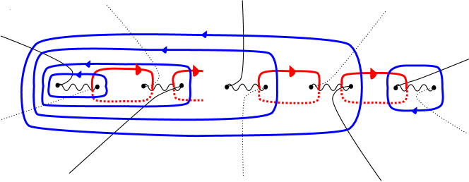
Figure 4: (colour online) A hyperelliptic curve $\Sigma$ is obtained by gluing together two sheets of this $s$-plane ($\mathbb{C}\cup\{\infty\}$) along the branch cuts (wavy lines) between $s_{1}$–$s_{2}$, $s_{3}$–$s_{4}$, $\cdots$, $s_{2g+1}$–$s_{2g+2}$; this picture is drawn for the case with $g=4$. Description of line bundles ${\cal L}^{\otimes k}$ requires branch cuts in the $U^{(s)}$ patch; the cuts for this purpose are drawn in thin (solid or dotted) lines in this figure. Thick grey (red) loops, from left to right, are the cycles $\alpha_{1}$, $\alpha_{2}$ (drawn partially), $\alpha_{g-1}$ and $\alpha_{g}$. Thick dark (blue) loops, from left to right, are $\beta^{1}$, $\beta^{2}$, $\beta^{g-1}$ and $\beta^{g}$; one more remaining loop in the thick dark (blue) line at the right end of this picture is $\beta^{{}^{\prime}g}$; $\beta^{g}$ and $\beta^{{}^{\prime}g}$ are isomorphic in $\Sigma$, but they are not within the $U^{(s)}$ patch.

Before getting into the study of monodromy, we first need to have a concrete construction of the cycles $\widetilde{C}^{i}$’s ($i=1,\cdots,g$), whose monodromy we are interested in. Math preparation is thus in order here. The line bundle $K_{\Sigma}={\cal L}^{\otimes 6}$ can be described by three Zariski open patches of $\Sigma$.

$$U^{(s)}:\quad t\neq 0,\infty;\qquad U^{(t)}:\quad P^{\prime}(s)\neq 0,\;s\neq\infty;\qquad U^{(\infty)}:\quad s\neq 0,s_{i}.$$ (91)

Sections of $K_{\Sigma}$ are written down in the form of $A=a^{(s)}ds$, $A^{(t)}dt$ and $A^{(\infty)}d(1/s)$ in the $U^{(s)}$, $U^{(t)}$ and $U^{(\infty)}$ patch, respectively; these trivialisation descriptions are identified by using transition functions:

$$a^{(t)}=\frac{2t}{P^{\prime}(s)}a^{(s)},\qquad a^{(\infty)}=(-s^{2})a^{(s)}.$$ (92)

$H^{0}(\Sigma;K_{\Sigma})$ is of $g$ dimensions, and are of the form

$$A_{6}^{(s)}ds=\frac{c_{0}+c_{1}s+\cdots+c_{g-1}s^{g-1}}{t}ds=\frac{c_{0}(1/s)^{g-1}+\cdots c_{g-1}}{(t/s^{g+1})}d(1/s)=A_{6}^{(\infty)}d(1/s).$$ (93)

The fibre coordinates $Y$ of ${\cal L}^{\otimes 3}$ and $X$ of ${\cal L}^{\otimes 2}$, for example, become $Y^{(s)}$, $Y^{(t)}$ and $Y^{(\infty)}$, and $X^{(s)}$, $X^{(t)}$ and $X^{(\infty)}$, respectively, in the trivialisation patches, and are identified between the overlapping patches as in

$$Y^{(t)}=\left(\frac{2t}{P^{\prime}(s)}\right)^{3/6}Y^{(s)},\qquad X^{(t)}=\left(\frac{2t}{P^{\prime}(s)}\right)^{2/6}X^{(s)}.$$ (94)

Branch cuts are introduced in these $U^{(s)}$, $U^{(t)}$ and $U^{(\infty)}$; see Figure 4 for the branch cuts in the $U^{(s)}$ patch; the coordinates $Y^{(s)}$ and $X^{(s)}$ at one point in $U^{(s)}\subset\Sigma$ and the coordinates $Y^{(s)^{\prime}}$ and $X^{(s)^{\prime}}$ at the same point that we reach after circling around a branch point (where $t=0$) by phase $+2\pi$ are identified through

$$Y^{(s)^{\prime}}=Y^{(s)}\times\zeta_{6}^{-3},\qquad X^{(s)^{\prime}}=X^{(s)}\times\zeta_{6}^{-2};\qquad\zeta_{6}:=e^{\frac{2\pi i}{6}}.$$ (95)

Fibre coordinates need to be identified through similar relations also across the branch cuts in $U^{(t)}$ and $U^{(\infty)}$. Equations (94) are made well-defined in this way. The same holds true also for the fibre coordinates $A_{3}$ and $A_{4}$.

Let us take a point $q\in U^{(s)}\subset\Sigma$. The local fourfold geometry $Y_{\rm local}$ has a three-dimensional fibre

$$Y^{(s)}A_{3}^{(s)}=X^{(s)}A_{4}^{(s)}+A_{6}^{(s)};$$ (96)

$Y^{(s)}$, $A_{3}^{(s)}$, $X^{(s)}$ and $A_{4}^{(s)}$ are coordinates, while $A_{6}^{(s)}$ is a parameter. This is a deformed conifold, and there is a canonical choice of compact three-cycle and a semi-canonical choice of non-compact three-cycle intersecting at one point; they are referred to as $A$-cycle and $B$-cycle; the choice of the $B$-cycle is not canonical, in that the $B$-cycle is deformed to be $B+A$ topologically, when the complex phase of the parameter $A_{6}^{(s)}$ changes as $A_{6}^{(s)}\longrightarrow A_{6}^{(s)}\times e^{i\alpha}$, $\alpha\in[0,2\pi]$, as well-known in deformed conifold.

Now, we are ready to provide description of the $2g$ remaining four-cycles, $\widetilde{C}^{i=1,\cdots,g}$ and $\widetilde{C}^{{}^{\prime}}_{j=1,\cdots,g}$ in $Y_{\rm local}$. Since this task is topological in nature, we can choose the parameter $A_{6}\in{\cal M}_{*}^{\rm local}$ arbitrarily; we choose it to be

$$A_{6}=A_{6}^{*}:=\epsilon\frac{(s-s_{*})^{g-1}}{t}ds,\qquad\qquad s_{2g+2}\ll s_{*}\in\mathbb{R}$$ (97)

for now. First of all, the cycles $\widetilde{A}_{i=1,\cdots,g}$ and $\widetilde{A}^{{}^{\prime}j=1,\cdots,g}$ are the $A$-cycle fibred over the one-cycles $\alpha_{i=1,\cdots,g}$ and $\beta^{j=1,\cdots,g}$ in $\Sigma$, as in the appendix C.1; see Figure 4 for how to choose the basis of $H_{1}(\Sigma;\mathbb{Z})$.

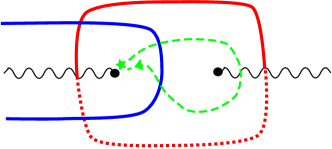
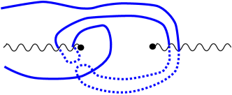
(a)		(b)

Figure 5: (colour online) (a) A loop $\gamma_{k}$ ($k=1,\cdots,g-1$) in the ${\cal M}_{*}^{\rm local}\cong\mathbb{C}^{g}$ parameter space is given by continuously changing the parameter $a_{k}$ in the $s$-plane, starting from $s=s_{2k}$, going around $s=s_{2k+1}$ and returning to $s=s_{2k}$, as shown by a dashed (green) arrow line in this picture. At the end of this deformation procedure, the loop $\beta^{k}$ has been deformed in the way shown in (b) by a thick solid (blue) line.

Secondly, for this choice of $A_{6}^{*}$, the cycles $\widetilde{B}_{\ell=1,\cdots,2g-3}$ are all located in the $s\sim s_{*}\gg s_{2g+2}$ region; we see after constructing $\widetilde{C}$’s that $\widetilde{B}_{\ell}$’s and $\widetilde{A}$–$\widetilde{C}$’s are mutually orthogonal in the intersection form. Finally, we claim that the $B$-cycle of the deformed conifold comes back to itself, not to $B+mA$ with $m\neq 0$, after a point $q\in\Sigma$ moves along any one of $\{\alpha_{i},\beta^{j}\}$. To verify this claim, first note that the loop $\beta^{k}$ crosses the branch cut in $U^{(s)}$ for $k$-times in the counter-clockwise direction; this means that the fibre coordinate of ${\cal L}^{\otimes a}$ at the end of a loop along $\beta^{k}$ is $\zeta_{6}^{-a\times k}=e^{-2\pi i\times\frac{a\cdot k}{6}}$ times the one at the beginning of the loop. The parameter $(A_{6}^{*})^{(s)}$, on the other hand, changes its phase by $e^{-2\pi ik}$ due to the factor $1/t$. Those two phases on both sides of (96) cancel, and there is no net change in the phase of the deformation parameter (not even a multiple of $2\pi$) along the loop $\beta^{k}$. Thus, the $B$-cycle comes back to itself. The $B$-cycle fibred over $\beta^{k}$ ($k=1,\cdots,g$) forms a four-cycle $\widetilde{C}^{k}$. Similarly, we note that the loop $\alpha_{k}$ crosse the branch cuts in $U^{(s)}$ for $(-1)$ times in the counter-clockwise direction. The parameter $(A_{6}^{*})^{(s)}$ changes its phase by $e^{+2\pi i}$ due to the factor $1/t$, on the other hand. Those two effects cancel, and there is no net change in the phase. Thus, the $B$-cycle comes back to itself at the end of the loop $\alpha_{k}$. This is how a four-cycle $\widetilde{C}^{{}^{\prime}}_{k}$ is obtained ($k=1,\cdots,g$). By construction, $\widetilde{A}_{i}\cdot\widetilde{C}^{j}=\delta_{i}^{\;j}$, $\widetilde{A}^{{}^{\prime}k}\cdot\widetilde{C}^{\prime}_{h}=\delta^{k}_{\;h}$, and the intersection number vanishes for all other combinations of $\widetilde{A}$’s and $\widetilde{C}$’s.

Finally, we study monodromy of those four-cycles in $Y_{\rm local}$. Monodromy is studied for loops departing and returning to a reference point in ${\cal M}_{*}^{\rm local}=\mathbb{C}^{g}$, and we choose

$$A_{6}=A_{6}^{**}:=\epsilon\frac{(s-s_{2})(s-s_{4})\cdots(s-s_{2(g-1)})}{t}ds$$ (98)

as the reference point., At this reference point, let $\widetilde{A}_{k}$ and $\widetilde{A}^{{}^{\prime}k}$ ($k=1,\cdots,g$) be the four-cycle given by the $A$-cycle along $\alpha_{k}$ and $\beta^{k}$, respectively. $g-1$ more four-cycles $\widetilde{C}^{k}$ ($k=1,\cdots,g-1$) are the $B$-cycle fibred over $\beta^{k}+k\alpha_{k}$ in $\Sigma$; this loop in $\Sigma$ crosses $+k$ times along $\beta^{k}$ and $k\times(-1)$ times along $k\alpha_{k}$, and there is no net change in the phase of $A_{6}^{**}$ along the loop. One more four-cycle, $\widetilde{C}^{g}$, is the $B$-cycle fibred over a one-cycle $\beta^{{}^{\prime}g}\sim\beta^{g}$ on $\Sigma$ shown in Figure 4. We will focus on monodromy associated with those $3g$ four-cycles.

It is convenient to adopt the following parameterisation of ${\cal M}_{*}^{\rm local}\cong H^{0}(\Sigma;K_{\Sigma})$:

$$A_{6}=\epsilon\frac{(s-a_{1})(s-a_{2})\cdots(s-a_{g-1})}{t}ds,\qquad\left\{(\epsilon,a_{1},\cdots,a_{g-1})\right\}\in\mathbb{C}^{g}.$$ (99)

The reference point $A_{6}^{**}$ corresponds to choosing $a_{k}=s_{2k}$ for $k=1,\cdots,g-1$. Loops $\gamma_{k}$ for $k=1,\cdots,g-1$ in ${\cal M}_{*}^{\rm local}$ are such that $a_{k}$ is changed continuously in the $s$-plane in the way designated in Figure 5 (a), while the value of $\epsilon$ and all other $a_{m}$’s ($m=1,\cdots,g-1$ but $m\neq k$) are held fixed. One can keep track of topology of the four-cycles $\widetilde{A}$’s and $\widetilde{C}$’s along the loop $\gamma_{k}$ in ${\cal M}_{*}^{\rm local}$, by deforming the one-cycles $\beta^{m}+m\alpha_{m}$ ($m=1,\cdots,g-1$) and $\beta^{{}^{\prime}g}$ so that the zero of $A_{6}^{(s)}$ is avoided. This is enough to conclude that all the $3g$ four-cycles, namely, $\widetilde{A}$’s, $\widetilde{A}^{\prime}$’s and $\widetilde{C}$’s, remain the same at the end of a loop $\gamma_{k}$ except $\widetilde{C}^{k}$. Furthermore, because the one-cycle $\beta^{k}$ needs to be deformed as in Figure 5 (b) at the end of the loop $\gamma_{k}$, there is a non-trivial monodromy

$$\gamma_{k}:\left(\widetilde{A}_{k},\widetilde{C}^{k}\right)\rightarrow\left(\widetilde{A}_{k},\widetilde{C}^{k}\right)\left(\begin{array}[]{cc}1&1\\ &1\end{array}\right),\qquad\left(\widetilde{A}_{m\neq k},\widetilde{A}^{{}^{\prime}j},\widetilde{C}^{m\neq k}\right)\rightarrow\left(\widetilde{A}_{m\neq k},\widetilde{A}^{{}^{\prime}j},\widetilde{C}^{m\neq k}\right).$$ (100)

We study monodromy along one more loop $\gamma_{\epsilon}$ in ${\cal M}_{*}^{\rm local}$, which is to change the phase of the parameter $\epsilon$ by $2\pi$, while all the $a_{m}$’s with $m=1,\cdots,g-1$ are held fixed. Topological cycles $\widetilde{A}_{k}$’s for $k=1,\cdots,g$ remain the same under the complex structure deformation along $\gamma_{\epsilon}$. Topological cycles $\widetilde{C}^{k}$’s are not, however. These cycles are all in the form of the $B$-cycle fibred over some one-cycle in $\Sigma$; after complex structure deformation along $\gamma_{\epsilon}$, the original $B$-cycle comes back as $B+A$-cycle. This means that

$$\gamma_{\epsilon}:\widetilde{C}^{k\neq g}\longmapsto\widetilde{C}^{k}+k\widetilde{A}_{k}+\widetilde{A}^{{}^{\prime}k},\qquad\widetilde{C}^{g}\longmapsto\widetilde{C}^{g}+\widetilde{A}^{{}^{\prime}g}.$$ (101)

This is enough to conclude that the period integrals depend on $\epsilon$ as

$$\Pi_{\widetilde{A}_{k}},\quad\Pi_{\widetilde{A}^{{}^{\prime}k}}\sim\epsilon,\qquad\Pi_{\widetilde{C}^{k\neq g}}\sim\left(\tau^{km}z_{m}+kz_{k}\right)\ln(\epsilon),\qquad\Pi_{\widetilde{C}^{g}}\sim\left(\tau^{gm}z_{m}\right)\ln(\epsilon).$$ (102)

It is a much more involved problem to determine the full monodromy group repreesnted on the space of $6g-3$ four-cycles, and also the period integrals. We do not do so in this article, since we do not need such a thorough analysis for the sketchy argument in the main text.

References

- [1] M. R. Douglas and S. Kachru, “Flux compactification,” Rev. Mod. Phys. 79 (2007) 733 [hep-th/0610102].
- [2] F. Denef, “Les Houches Lectures on Constructing String Vacua,” arXiv:0803.1194 [hep-th].
- [3] S. Ashok and M. R. Douglas, “Counting flux vacua,” JHEP 0401 (2004) 060 [hep-th/0307049].
- [4] F. Denef and M. R. Douglas, “Distributions of flux vacua,” JHEP 0405 (2004) 072 [hep-th/0404116].
- [5] A. P. Braun, Y. Kimura and T. Watari, “The Noether-Lefschetz problem and gauge-group-resolved landscapes: F-theory on K3 K3 as a test case,” JHEP 1404 (2014) 050 [arXiv:1401.5908 [hep-th]].
- [6] A. P. Braun and T. Watari, “Distribution of the Number of Generations in Flux Compactifications,” Phys. Rev. D 90 (2014) 12, 121901 [arXiv:1408.6156 [hep-ph]]; “The Vertical, the Horizontal and the Rest: anatomy of the middle cohomology of Calabi-Yau fourfolds and F-theory applications,” JHEP 1501 (2015) 047 [arXiv:1408.6167 [hep-th]].
- [7] S. Weinberg, “Supersymmetry at Ordinary Energies. 1. Masses and Conservation Laws,” Phys. Rev. D 26 (1982) 287; A. E. Faraggi, “Proton stability in superstring derived models,” Nucl. Phys. B 428 (1994) 111 [hep-ph/9403312].
- [8] M. Dine and Z. Sun, “R symmetries in the landscape,” JHEP 0601 (2006) 129 [hep-th/0506246]. M. Dine, “Naturalness Under Stress,” arXiv:1501.01035 [hep-ph].
- [9] R. Tatar and T. Watari, “Proton decay, Yukawa couplings and underlying gauge symmetry in string theory,” Nucl. Phys. B 747 (2006) 212 [hep-th/0602238].
- [10] M. Kuriyama, H. Nakajima and T. Watari, “Theoretical Framework for R-parity Violation,” Phys. Rev. D 79 (2009) 075002 [arXiv:0802.2584 [hep-ph]].
- [11] R. Tatar, Y. Tsuchiya and T. Watari, “Right-handed Neutrinos in F-theory Compactifications,” Nucl. Phys. B 823 (2009) 1 [arXiv:0905.2289 [hep-th]].
- [12] Y. Nir and N. Seiberg, “Should squarks be degenerate?,” Phys. Lett. B 309 (1993) 337 [hep-ph/9304307].
- [13] S. Cecotti, C. Cordova, J. J. Heckman and C. Vafa, “T-Branes and Monodromy,” JHEP 1107 (2011) 030 [arXiv:1010.5780 [hep-th]].
- [14] R. Donagi and M. Wijnholt, “Model Building with F-Theory,” Adv. Theor. Math. Phys. 15 (2011) 1237 [arXiv:0802.2969 [hep-th]].
- [15] C. Beasley, J. J. Heckman and C. Vafa, “GUTs and Exceptional Branes in F-theory - I,” JHEP 0901 (2009) 058 [arXiv:0802.3391 [hep-th]].
- [16] S. H. Katz and C. Vafa, “Matter from geometry,” Nucl. Phys. B 497 (1997) 146 [hep-th/9606086].
- [17] J. Marsano, N. Saulina and S. Schafer-Nameki, “Monodromies, Fluxes, and Compact Three-Generation F-theory GUTs,” JHEP 0908 (2009) 046 [arXiv:0906.4672 [hep-th]]; “Compact F-theory GUTs with U(1) (PQ),” JHEP 1004 (2010) 095 [arXiv:0912.0272 [hep-th]].
- [18] H. Hayashi, T. Kawano, Y. Tsuchiya and T. Watari, “More on Dimension-4 Proton Decay Problem in F-theory – Spectral Surface, Discriminant Locus and Monodromy,” Nucl. Phys. B 840 (2010) 304 [arXiv:1004.3870 [hep-th]].
- [19] T. W. Grimm and T. Weigand, “On Abelian Gauge Symmetries and Proton Decay in Global F-theory GUTs,” Phys. Rev. D 82 (2010) 086009 [arXiv:1006.0226 [hep-th]].
- [20] D. R. Morrison and C. Vafa, “Compactifications of F theory on Calabi-Yau threefolds. 2.,” Nucl. Phys. B 476 (1996) 437 [hep-th/9603161].
- [21] V. Braun, T. W. Grimm and J. Keitel, “New Global F-theory GUTs with U(1) symmetries,” JHEP 1309 (2013) 154 [arXiv:1302.1854 [hep-th]].
- [22] V. Braun, T. W. Grimm and J. Keitel, “Geometric Engineering in Toric F-Theory and GUTs with U(1) Gauge Factors,” JHEP 1312 (2013) 069 [arXiv:1306.0577 [hep-th]].
- [23] For examples, D. Klevers, D. K. Mayorga Pena, P. K. Oehlmann, H. Piragua and J. Reuter, “F-Theory on all Toric Hypersurface Fibrations and its Higgs Branches,” JHEP 1501 (2015) 142 [arXiv:1408.4808 [hep-th]], C. Lawrie, S. Schafer-Nameki and J. M. Wong, “F-theory and All Things Rational: Surveying U(1) Symmetries with Rational Sections,” arXiv:1504.05593 [hep-th], and references therein.
- [24] E. Witten, “Phase transitions in M theory and F theory,” Nucl. Phys. B 471 (1996) 195 [hep-th/9603150]. P. Mayr, “Mirror symmetry, N=1 superpotentials and tensionless strings on Calabi-Yau four folds,” Nucl. Phys. B 494 (1997) 489 [hep-th/9610162]. P. Candelas, D. E. Diaconescu, B. Florea, D. R. Morrison and G. Rajesh, “Codimension three bundle singularities in F theory,” JHEP 0206 (2002) 014 [hep-th/0009228].
- [25] S. Sethi, C. Vafa and E. Witten, “Constraints on low dimensional string compactifications,” Nucl. Phys. B 480 (1996) 213 [hep-th/9606122]. A. Klemm, B. Lian, S. S. Roan and S. T. Yau, “Calabi-Yau fourfolds for M theory and F theory compactifications,” Nucl. Phys. B 518 (1998) 515 [hep-th/9701023]. M. Kreuzer and H. Skarke, “Calabi-Yau four folds and toric fibrations,” J. Geom. Phys. 26 (1998) 272 [hep-th/9701175].
- [26] W. Taylor, “On the Hodge structure of elliptically fibered Calabi-Yau threefolds,” JHEP 1208 (2012) 032 [arXiv:1205.0952 [hep-th]]. L. B. Anderson and W. Taylor, “Geometric constraints in dual F-theory and heterotic string compactifications,” JHEP 1408 (2014) 025 [arXiv:1405.2074 [hep-th]]. J. Halverson and W. Taylor, “-bundle bases and the prevalence of non-Higgsable structure in 4D F-theory models,” arXiv:1506.03204 [hep-th].
- [27] J. Gray, A. S. Haupt and A. Lukas, “All Complete Intersection Calabi-Yau Four-Folds,” JHEP 1307 (2013) 070 [arXiv:1303.1832 [hep-th]]. J. Gray, A. S. Haupt and A. Lukas, “Topological Invariants and Fibration Structure of Complete Intersection Calabi-Yau Four-Folds,” JHEP 1409 (2014) 093 [arXiv:1405.2073 [hep-th]].
- [28] D. R. Morrison and W. Taylor, “Classifying bases for 6D F-theory models,” Central Eur. J. Phys. 10 (2012) 1072 [arXiv:1201.1943 [hep-th]]. D. R. Morrison and W. Taylor, “Non-Higgsable clusters for 4D F-theory models,” JHEP 1505 (2015) 080 [arXiv:1412.6112 [hep-th]].
- [29] I. Affleck, M. Dine and N. Seiberg, “Dynamical Supersymmetry Breaking in Four-Dimensions and Its Phenomenological Implications,” Nucl. Phys. B 256 (1985) 557.
- [30] R. Bousso and J. Polchinski, “Quantization of four form fluxes and dynamical neutralization of the cosmological constant,” JHEP 0006 (2000) 006 [hep-th/0004134].
- [31] O. DeWolfe, A. Giryavets, S. Kachru and W. Taylor, “Enumerating flux vacua with enhanced symmetries,” JHEP 0502 (2005) 037 [hep-th/0411061].
- [32] E. Witten, “Symmetry Breaking Patterns in Superstring Models,” Nucl. Phys. B 258 (1985) 75; “New Issues in Manifolds of SU(3) Holonomy,” Nucl. Phys. B 268 (1986) 79.
- [33] H. Georgi and S. L. Glashow, “Unity of All Elementary Particle Forces,” Phys. Rev. Lett. 32 (1974) 438.
- [34] L. Lin and T. Weigand, “Towards the Standard Model in F-theory,” Fortsch. Phys. 63 (2015) 2, 55 [arXiv:1406.6071 [hep-th]].
- [35] A. Grassi, J. Halverson, J. Shaneson and W. Taylor, “Non-Higgsable QCD and the Standard Model Spectrum in F-theory,” JHEP 1501 (2015) 086 [arXiv:1409.8295 [hep-th]].
- [36] M. R. Douglas, D. S. Park and C. Schnell, “The Cremmer-Scherk Mechanism in F-theory Compactifications on K3 Manifolds,” JHEP 1405 (2014) 135 [arXiv:1403.1595 [hep-th]]. D. R. Morrison and W. Taylor, “Sections, multisections, and U(1) fields in F-theory,” arXiv:1404.1527 [hep-th]. G. Martini and W. Taylor, “6D F-theory models and elliptically fibered Calabi-Yau threefolds over semi-toric base surfaces,” JHEP 1506 (2015) 061 [arXiv:1404.6300 [hep-th]].
- [37] A. Giryavets, S. Kachru and P. K. Tripathy, “On the taxonomy of flux vacua,” JHEP 0408 (2004) 002 [hep-th/0404243].
- [38] J. P. Conlon and F. Quevedo, “On the explicit construction and statistics of Calabi-Yau flux vacua,” JHEP 0410 (2004) 039 [hep-th/0409215].
- [39] T. Eguchi and Y. Tachikawa, “Distribution of flux vacua around singular points in Calabi-Yau moduli space,” JHEP 0601 (2006) 100 [hep-th/0510061].
- [40] D. Cox and S. Katz, “Mirror symmetry and algebraic geometry,” American Mathematical Society, 1999.
- [41] K. Intriligator, H. Jockers, P. Mayr, D. R. Morrison and M. R. Plesser, “Conifold Transitions in M-theory on Calabi-Yau Fourfolds with Background Fluxes,” Adv. Theor. Math. Phys. 17 (2013) 601 [arXiv:1203.6662 [hep-th]].
- [42] H. Hayashi, T. Kawano, R. Tatar and T. Watari, “Codimension-3 Singularities and Yukawa Couplings in F-theory,” Nucl. Phys. B 823 (2009) 47 [arXiv:0901.4941 [hep-th]].
- [43] J. J. Heckman and C. Vafa, “Flavor Hierarchy From F-theory,” Nucl. Phys. B 837 (2010) 137 [arXiv:0811.2417 [hep-th]].
- [44] S. Cecotti, M. C. N. Cheng, J. J. Heckman and C. Vafa, “Yukawa Couplings in F-theory and Non-Commutative Geometry,” arXiv:0910.0477 [hep-th].
- [45] H. Hayashi, T. Kawano, Y. Tsuchiya and T. Watari, “Flavor Structure in F-theory Compactifications,” JHEP 1008 (2010) 036 [arXiv:0910.2762 [hep-th]].
- [46] C. Cordova, “Decoupling Gravity in F-Theory,” Adv. Theor. Math. Phys. 15 (2011) 689 [arXiv:0910.2955 [hep-th]].
- [47] for example, W. Buchmuller, K. Hamaguchi, O. Lebedev and M. Ratz, “Supersymmetric Standard Model from the Heterotic String (II),” Nucl. Phys. B 785 (2007) 149 [hep-th/0606187].
- [48] J. L. Bourjaily, “Local Models in F-Theory and M-Theory with Three Generations,” arXiv:0901.3785 [hep-th].
- [49] J. Marsano, N. Saulina and S. Schafer-Nameki, “F-theory Compactifications for Supersymmetric GUTs,” JHEP 0908 (2009) 030 [arXiv:0904.3932 [hep-th]].
- [50] J. P. Conlon and E. Palti, “Aspects of Flavour and Supersymmetry in F-theory GUTs,” JHEP 1001 (2010) 029 [arXiv:0910.2413 [hep-th]].
- [51] F. Marchesano and L. Martucci, “Non-perturbative effects on seven-brane Yukawa couplings,” Phys. Rev. Lett. 104 (2010) 231601 [arXiv:0910.5496 [hep-th]]. C. C. Chiou, A. E. Faraggi, R. Tatar and W. Walters, “T-branes and Yukawa Couplings,” JHEP 1105 (2011) 023 [arXiv:1101.2455 [hep-th]]. A. Font, L. E. Ibanez, F. Marchesano and D. Regalado, “Non-perturbative effects and Yukawa hierarchies in F-theory SU(5) Unification,” JHEP 1303 (2013) 140 [JHEP 1307 (2013) 036] [arXiv:1211.6529 [hep-th]]. L. Aparicio, A. Font, L. E. Ibanez and F. Marchesano, “Flux and Instanton Effects in Local F-theory Models and Hierarchical Fermion Masses,” JHEP 1108 (2011) 152 [arXiv:1104.2609 [hep-th]]. A. Font, F. Marchesano, D. Regalado and G. Zoccarato, “Up-type quark masses in SU(5) F-theory models,” JHEP 1311 (2013) 125 [arXiv:1307.8089 [hep-th]].
- [52] L. Randall and D. Simmons-Duffin, “Quark and Lepton Flavor Physics from F-Theory,” arXiv:0904.1584 [hep-ph].
- [53] L. J. Hall, H. Murayama and N. Weiner, “Neutrino mass anarchy,” Phys. Rev. Lett. 84 (2000) 2572 [hep-ph/9911341]. N. Haba and H. Murayama, “Anarchy and hierarchy,” Phys. Rev. D 63 (2001) 053010 [hep-ph/0009174].
-
[54]
N. Arkani-Hamed and S. Dimopoulos,
“New origin for approximate symmetries from distant breaking in extra dimensions,”
Phys. Rev. D 65 (2002) 052003
[hep-ph/9811353].
N. Arkani-Hamed and M. Schmaltz, “Hierarchies without symmetries from extra dimensions,” Phys. Rev. D 61 (2000) 033005 [hep-ph/9903417]. - [55] L. J. Hall, M. P. Salem and T. Watari, “Quark and Lepton Masses from Gaussian Landscapes,” Phys. Rev. Lett. 100 (2008) 141801 [arXiv:0707.3444 [hep-ph]]. L. J. Hall, M. P. Salem and T. Watari, “Statistical Understanding of Quark and Lepton Masses in Gaussian Landscapes,” Phys. Rev. D 76 (2007) 093001 [arXiv:0707.3446 [hep-ph]]. L. J. Hall, M. P. Salem and T. Watari, “Neutrino mixing and mass hierarchy in Gaussian landscapes,” Phys. Rev. D 79 (2009) 025010 [arXiv:0810.2561 [hep-th]].
- [56] D. Cremades, L. E. Ibanez and F. Marchesano, “Computing Yukawa couplings from magnetized extra dimensions,” JHEP 0405 (2004) 079 [hep-th/0404229].
- [57] Math textbooks, such as I. Shafarevich, “Basic Algebraic Geometry,” Chapter I, section 1.4, Shpringer–Verlag, 1988.
- [58] M. Cvetic, D. Klevers and H. Piragua, “F-Theory Compactifications with Multiple U(1)-Factors: Constructing Elliptic Fibrations with Rational Sections,” JHEP 1306 (2013) 067 [arXiv:1303.6970 [hep-th]].
- [59] A. Hebecker, P. Mangat, F. Rompineve and L. T. Witkowski, “Tuning and Backreaction in F-term Axion Monodromy Inflation,” Nucl. Phys. B 894 (2015) 456 [arXiv:1411.2032 [hep-th]].
- [60] A. Grassi and V. Perduca, “Weierstrass models of elliptic toric hypersurfaces and symplectic cuts,” Adv. Theor. Math. Phys. 17 (2013) 741 [arXiv:1201.0930 [math.AG]].
- [61] T. W. Grimm and H. Hayashi, “F-theory fluxes, Chirality and Chern-Simons theories,” JHEP 1203 (2012) 027 [arXiv:1111.1232 [hep-th]].
- [62] M. Bershadsky, T. Pantev and V. Sadov, “F theory with quantized fluxes,” Adv. Theor. Math. Phys. 3 (1999) 727 [hep-th/9805056].
- [63] D. R. Morrison and D. S. Park, “F-Theory and the Mordell-Weil Group of Elliptically-Fibered Calabi-Yau Threefolds,” JHEP 1210 (2012) 128 [arXiv:1208.2695 [hep-th]].
- [64] D. S. Park and W. Taylor, “Constraints on 6D Supergravity Theories with Abelian Gauge Symmetry,” JHEP 1201 (2012) 141 [arXiv:1110.5916 [hep-th]].
- [65] P. Candelas and A. Font, “Duality between the webs of heterotic and type II vacua,” Nucl. Phys. B 511 (1998) 295 [hep-th/9603170].
- [66] M. Esole and S. T. Yau, “Small resolutions of SU(5)-models in F-theory,” Adv. Theor. Math. Phys. 17 (2013) 1195 [arXiv:1107.0733 [hep-th]].
- [67] M. Bershadsky, K. A. Intriligator, S. Kachru, D. R. Morrison, V. Sadov and C. Vafa, “Geometric singularities and enhanced gauge symmetries,” Nucl. Phys. B 481 (1996) 215 [hep-th/9605200].
- [68] D. Berenstein, “Branes versus GUTS: Challenges for string inspired phenomenology,” hep-th/0603103.
- [69] S. Katz, P. Mayr and C. Vafa, “Mirror symmetry and exact solution of 4-D N=2 gauge theories: 1.,” Adv. Theor. Math. Phys. 1 (1998) 53 [hep-th/9706110]. P. Berglund and P. Mayr, “Heterotic string / F theory duality from mirror symmetry,” Adv. Theor. Math. Phys. 2 (1999) 1307 [hep-th/9811217].
- [70] H. Hayashi, R. Tatar, Y. Toda, T. Watari and M. Yamazaki, “New Aspects of Heterotic–F Theory Duality,” Nucl. Phys. B 806 (2009) 224 [arXiv:0805.1057 [hep-th]].
- [71] R. Donagi and M. Wijnholt, “Higgs Bundles and UV Completion in F-Theory,” Commun. Math. Phys. 326 (2014) 287 [arXiv:0904.1218 [hep-th]].