Bounding the Heat Trace of a Calabi-Yau Manifold

arXiv:yymm.nnnnn [hep-th]

June 2015 

Email: marc-antoine.fiset@mail.mcgill.ca, johannes.walcher@mcgill.ca

1 Introduction

Perturbation theory approximates the space of solutions of string theory by the space of two-dimensional conformal field theories satisfying certain conditions on the chiral algebra, such as an appropriate central charge or extended supersymmetry, that allow a consistent coupling to two-dimensional gravity, and guarantee perturbative consistency and finiteness of the space-time theory [1, 2].

Non-perturbative quantum corrections [3] and dualities [4] change both the local and the global details of this picture of the space of string vacua, and will eventually stabilize even a non-supersymmetric vacuum [5]. However, these modifications do not address the central issue of finiteness of the String Landscape [6], which, in the absence of other principles, would provide a viable approach to string phenomenology [7].

In recent years, a revival of the conformal bootstrap program has led to remarkable progress on a priori constraints on the operator content of certain types of conformal field theories. Of particular interest for the space of string vacua are the results of Hellerman and Schmidt-Colinet [8], and Keller and Ooguri [9], SCHOK: Exploiting only the constraint of modular invariance of the torus partition function (and, in the supersymmetric case, of the elliptic genus), these works have shown that there exists an intimate relationship between the number of marginal and relevant operators in two-dimensional (super-)conformal field theories. Besides its phenomenological relevance as a starting point for phenomenological finiteness in string theory, a strict upper bound on the number of marginal operators of a SCFT of central charge $\hat{c}=3$ would imply the existence of an upper bound on the dimension of cohomology groups of Calabi-Yau threefolds (and hence their Euler number), which is a hopeful, but largely open, mathematical conjecture.

In the present note, we explore in some detail the geometric ramifications of the SCHOK bound, as it applies to conformal field theories defined as the infrared fixed point of a Calabi-Yau sigma model. On the one hand, marginal deformations of such a CFT are in one-to-one correspondence with certain elements of the cohomology groups of the underlying manifold [10]. The associated harmonic forms can be identified with the supersymmetric ground states in the Hilbert space, which can be reached by spectral flow from the chiral ring spanned by the marginal operators [10]. This data also controls the massless spectrum of the space-time theory that results upon compactification of the ten-dimensional super-string on the Calabi-Yau.

On the other hand, relevant operators of the CFT correspond to states with negative worldsheet energy, not far above the tachyonic ground state. In a supersymmetric string compactification, such states are eliminated by the GSO projection, and do not actually enter the space-time theory at all. Nevertheless, they are present in the conformal field theory before GSO projection, and, by the SCHOK argument, allow some control over the space of marginal operators that do survive the GSO projection, and hence, the massless spectrum.

An important feature of this situation is that while the number of marginal operators is of cohomological nature (“BPS”) and hence does not vary over the smooth part of the moduli space (corresponding to space-time theories without extra, non-perturbative, massless states), the number of relevant operators, and their conformal dimensions, are moduli-dependent quantities. It is natural to ask whether the freedom that results from this distinction can be exploited to yield additional information on the spectrum of such conformal field theories.

The main idea of the present paper goes back to a question that arose in [11]: Are there any interesting constraints on the number of relevant operators that depend on a geometric origin of the conformal field theory, but that are independent of other, topological data such as the number of marginal deformations? What sorts of constraints on the massless spectrum can be derived from these results?

In the perturbative $\alpha^{\prime}$- (large-volume/small-curvature) expansion of the sigma model, the lightest string states are those without any oscillators excited, i.e., they involve only the variables describing the motion of the center of mass of the string on the manifold. Therefore, the questions about the number of relevant operators of the conformal field theory become questions of classical spectral geometry. We claim two main results.

First, we will argue, following [11], that an upper bound on the trace of the heat kernel of the Calabi-Yau manifold at large temperature (or small time), possibly together with bounds on qualitatively similar quantities, would be a sufficient constraint on the light spectrum of the resulting CFT to complement the SCHOK bound. Importantly, this bound need not hold everywhere in the moduli space of Ricci-flat metrics (and we do not expect that it does), but it should be uniform in the topology of the manifold, in a sense that we will explain.

As far as we know, no bound of this nature is presently available in the spectral geometry literature. There exists, of course, a standard large temperature expansion of the trace of the heat kernel going back to Weyl. However, the asymptotic nature of this expansion makes it insufficient for bounding purposes: The expansion coefficients are integrals of local curvature invariants of higher and higher order, so that estimating the remainder requires rescaling the metric to smooth out regions of large curvature. This, however, requires that the volume be large, and implies that the leading Weyl term cannot be controlled in a uniform fashion.

To investigate this issue, we study the spectrum of the scalar Laplacian and the behaviour of the heat trace in the regime in which the manifold develops a curvature singularity, but without relying on the asymptotic expansion previously mentioned. For concreteness, we focus on the approach to the conifold singularity of a Calabi-Yau threefold [12] “from the resolved side”, but the structure of the argument will make it clear that more general singularities should not be very different. We formulate the problem in terms of spectral continuity under the confluence of Heun eigenfunctions. The high order WKB analysis of these solutions suggests an explanation of the smooth behaviour observed in the high curvature limit.

Our second result is then the conclusion that not only do regions of large curvature not prevent the existence of a uniform bound, but that in fact degenerations of the manifold could be a useful starting point to obtain a uniform bound on the number of relevant operators, as long as one makes sure that the curvature remains below string scale in order to control the perturbative and non-perturbative $\alpha^{\prime}$-corrections.

2 The SCHOK Bound

In a remarkable paper [8], Hellerman and Schmidt-Colinet have shown how modular invariance of the torus partition function can be exploited for the purpose of deriving universal bounds on state degeneracies and related thermodynamic quantities in 2-dimensional conformal field theories.

Among the many interesting results of [8] is the statement that a local conformal field theory of total central charge $c_{\rm tot}=c_{L}+c_{R}<48$ and without relevant operators (operators of conformal dimension strictly between $0$ and $2$) can have no more than

$$\frac{c_{L}+c_{R}}{48-c_{L}-c_{R}}{\it e}^{4\pi}-2$$ (2.1)

marginal operators (operators of conformal dimension exactly equal to $2$).

The basic idea for deriving (2.1) is to restrict the modular invariant torus partition function $\mathcal{Z}(\tau)$ to purely imaginary $\tau={\it i}\beta/(2\pi)$, for which $\mathcal{Z}(\tau)$ becomes the thermodynamic partition function $\mathcal{Z}(\beta)=\sum_{n}{\it e}^{-\beta E_{n}}$ at temperature $1/\beta$ , and to expand around the self-dual point $\beta=2\pi$. To first order, invariance under $\beta\to(2\pi)^{2}/\beta$ entails a vanishing derivative, i.e.,

$$\left.\frac{d}{d\beta}\right|_{\beta=2\pi}\mathcal{Z}(\beta)=\sum_{n}E_{n}{\it e}^{-2\pi E_{n}}=0$$ (2.2)

One then notes that for sufficiently small central charge, the marginal operators contribute states with positive energy in (2.2). This contribution must be balanced by the states of negative energy. Without relevant operators, the only state of negative energy is the vacuum. This observation then yields the bound (2.1). An immediate generalization of this statement that is implicit in [8] is the fact that the number of marginal operators is bounded from above in terms of the number of operators that are above a certain level of relevance. In fact, the above bound is only interesting when $c_{\rm tot}\gtrsim 18.27$ for otherwise the CFT necessarily has relevant operators, as shown in ref. [13]. For smaller values of the central charge, the more general bound still obtains.

These ideas have been developed in a quantitative way ref. [9]. Keller and Ooguri consider 2-dimensional conformal field theories with ${\cal N}=2$ worldsheet supersymmetry of central charge $\hat{c}=3$ and all R-charges in the Neveu-Schwarz sector integral. The strategy outlined above yields better results after organizing the contributions into the various representations of the ${\cal N}=2$ superconformal algebra extended by the spectral flow (the Odake algebra). As is well-known, exactly marginal operators in ${\cal N}=2$ SCFT arise from chiral and antichiral primary fields (BPS representations of the ${\cal N}=2$ algebra), and, as shown in [9], make a positive contribution to the suitably weighted vanishing partition function. When the ${\cal N}=2$ superconformal field theory describes the IR fixed point of a Calabi-Yau sigma model, the number of marginal operators from chiral or twisted chiral representations is given by the Hodge numbers $h^{2,1}$ and $h^{1,1}$ of the Calabi-Yau, respectively; so one uses this notation also for the generic such SCFT. On the other hand, for central charge $\hat{c}=3$, negative contributions to the partition function come only from non-BPS primaries of sufficiently small conformal dimension $\Delta_{\rm total}$. Balancing the positive and negative contributions yields a bound much as in the non-supersymmetric case.

The main result of [9] can be written in the form

$$\#\{\text{non-BPS primaries with $\Delta_{\rm total}\leq 0.655\ldots$}\}\geq\frac{1}{522.0\ldots}\bigl{(}h^{1,1}+h^{2,1}-492.6\ldots\bigr{)}$$ (2.3)

It states that the spectrum of conformal field theories with total Hodge number $h^{1,1}+h^{2,1}$ sufficiently large must contain non-BPS primary states of conformal dimension less than $0.655\ldots$, and that the number of such primary states grows at least linearly in the total Hodge number. Equivalently, the number of marginal operators is bounded from above by a linear function of the number of sufficiently relevant operators.

It is worthwhile pointing out that the bound (2.3) is not necessarily optimal. Other variants on the idea of [8] might yield further refinements of the basic bound. Our goal is to explore the question whether it is possible by independent methods to obtain a further upper bound on the number of relevant operators, which could then, in combination with the SCHOK bound, be used to bound the number of marginal deformations in absolute terms.

We note that if any of these sufficiently relevant non-BPS operators survived the GSO projection in string theory, they would give rise to tachyonic states in space-time. Although they do of course not survive the GSO projection, we will therefore refer to the operators on the LHS of (2.3) as “counter-factual tachyons”, or “tachyons” for short. For the following discussion of supplemental geometric bounds, it will be convenient to summarize and remember the SCHOK bound as the statement that for fixed central charge, there exist constants $C_{0}$, $C_{1}$ such that in any ${\cal N}=2$ SCFT of that given central charge, the number $N_{\rm marginal}$ of exactly marginal BPS operators is bounded linearly by the number of tachyons, i.e.,

$$N_{\rm marginal}<C_{0}+C_{1}\cdot N_{\rm tachyons}$$ (2.4)

Below, we will be mostly concerned with the regime $N_{\rm marginal},N_{\rm tachyons}\gg 1$. We can then drop $C_{0}$ from the above statement without penalty.

3 Reduction

The SCHOK bound (2.4) becomes even more interesting when we consider it not for isolated conformal field theories, but for the entire family parameterized by the vevs of the marginal operators. Indeed, while the LHS is constant in the smooth part of the moduli space of ${\cal N}=2$ SCFT, the RHS is a priori a strongly moduli dependent quantity. The inequality of course must hold everywhere on moduli space, and we can use this freedom to look for regions in the moduli space in which the number of relevant operators is especially small, or else easy to estimate and bound.

Consider in particular an ${\cal N}=2$ SCFT of $\hat{c}=3$ that can be deformed into a phase in which it can be defined by a supersymmetric sigma model into a Calabi-Yau threefold $X$. Then, the number of marginal operators is given by the dimensions of the Dolbeault cohomology groups $H^{1,1}(X)$, parameterizing Kähler deformations, and $H^{2,1}(X)$, parameterizing complex structure deformations. Together, $H^{1,1}(X)\oplus H^{2,1}(X)$ is the tangent space to the space of Ricci-flat Kähler metrics on $X$ (Yau’s theorem).

On the other hand, to leading order in the $\alpha^{\prime}$-expansion of the string worldsheet theory (this is, morally speaking, the “supergravity approximation”), any would-be tachyonic states must be understood to arise by “Kaluza-Klein reduction” of the center-of-mass motion of the string with at most one $\psi^{\mu}_{-1/2}$ oscillator excited. In first approximation, the conformal dimensions of primaries, $\Delta_{n}$, are given by the eigenvalues, $\lambda_{n}$, of the Laplacian acting on scalar or vector-valued wavefunctions on $X$,

$$\Delta_{n}=\alpha^{\prime}\lambda_{n}+\cdots$$ (3.1)

In the limit in moduli space in which the volume of $X$ becomes very large, the eigenvalues accumulate at zero, so that the bound (2.3) will be trivially satisfied. Indeed, the LHS is just the dimension of the moduli space, and of course constant in the limit.

Conversely, the bound becomes potentially stringent if we can deform the manifold to a region in the moduli space of Ricci-flat metrics in which the number of low-lying eigenvalues of the Laplace operator is small. Intuitively, this will happen for a manifold of small volume. Unfortunately, in the small volume limit, the supergravity approximation will break down, $\alpha^{\prime}$-corrections will become large, and we will not be able to estimate the number of tachyons by counting eigenvalues of geometric operators. (By flat space intuition, the light spectrum will be dominated by winding modes in this regime [14].)

The strategy we advocate is to look for an intermediate regime in which the supergravity approximation is valid (say, the curvature radius and volume of the manifold are large in string units) yet the manifold is not so large that the continuum of states has fully materialized. Of course, a bound on the number of relevant operators in the CFT that one might obtain in this regime will be far from optimal. On the other hand, assuming (3.1) reduces the problem to a question amenable to exact mathematical analysis, which we discuss in the following sections. The problem in this regime remains non-trivial and highlights what we believe are the essential challenges in bounding the number of relevant operators more generally.

The replacement of the 2-d sigma model by its point-particle approximation itself is difficult to justify rigorously. There exists substantial evidence for the conjecture that a Calabi-Yau sigma model flows to an ${\cal N}=2$ SCFT in the infrared that admits an independent, and mathematically rigorous, construction in certain cases. This evidence is based on a comparison of the massless spectrum, i.e., the cohomology of the manifold, which is BPS and therefore protected by supersymmetry against renormalization, and on the general structure of higher-order terms in the $\beta$-function of ${\cal N}=2$ sigma models. For the non-BPS spectrum however, the perturbative $\alpha^{\prime}$-expansion (3.1) is not expected to be better than standard asymptotic expansions in quantum field theory. On the other hand, and this is an important distinction to the discussion in the following sections, the corrections are local in target space, and expected to be uniformly suppressed under the assumption that the curvature radius is large in string units. Related issue in a similar regime, albeit with somewhat different aims, were discussed recently in [14].

4 On Uniform Bounds

Given (2.4), in order to bound the dimension of moduli space, $N_{\rm marginal}$, of ${\cal N}=2$ SCFTs, it is enough to find, in the moduli space of deformations of any given SCFT, a point or region in which $N_{\rm tachyons}$ is bounded by some universal constant. Let us recall that $N_{\rm tachyons}$ is defined as the number of primary states with conformal dimension below $0.655\ldots$, see (2.3).

As explained in the previous section, we will restrict to those ${\cal N}=2$ SCFTs which have a Calabi-Yau phase in their moduli space, and we will look for the relevant region in the vicinity of the large-volume regime. We will assume that the conformal dimensions of relevant operators in the CFT can be approximated by the low-lying eigenvalues of the Laplace operator of the Ricci-flat metric on the Calabi-Yau, eq. (3.1), given that the curvature radius is large in string units. We will for simplicity restrict to scalar wavefunctions. We expect vector-valued wavefunctions to behave qualitatively similarly as long as the manifold is simply connected. Forms of higher degree and other geometric operators are not expected to play a role since the corresponding modes are already massive in the flat space limit.

For the geometric analysis, it is sometimes convenient to study instead of the distribution of eigenvalues itself, its Laplace transform,

$$Z_{X}(t)=\sum_{n}{\it e}^{-t\lambda_{n}}={\rm Tr}{\it e}^{-t\Delta}$$ (4.1)

which is otherwise known as the trace of the heat kernel in the literature. We may intuitively identify it as the point-particle approximation to the full stringy partition function. Here,

$$\Delta=-\frac{1}{\sqrt{g}}\frac{\partial}{\partial x^{I}}g^{IJ}\sqrt{g}\frac{\partial}{\partial x^{J}}$$ (4.2)

is the (positive-definite) scalar Laplacian on $X$, with metric $g_{IJ}$.

To reformulate the bound in terms of $Z_{X}(t)$, we note that for any fixed $t_{*}$, $Z_{X}(t_{*})$ is bounded below by ${\it e}^{-1}$ times the number of eigenvalues smaller than $1/t_{*}$. Therefore, for $t_{*}=\alpha^{\prime}/0.655\ldots$, an upper bound on $Z_{X}(t_{*})$ implies an upper bound on $N_{\rm tachyons}$. In the regime of concern, we may then write the SCHOK bound (2.4) as

$$N_{\rm marginal}<{\it e}\cdot C_{1}\cdot Z_{X}(t_{*}).$$ (4.3)

Note that we are assuming that $X$ is large and weakly curved in string units, but that we are otherwise allowing arbitrary (Kähler and complex structure) deformations of the metric in order to make $Z_{X}(t_{*})$ as small as possible.

Then, as an approximation to an effective bound on the number of tachyons, we may ask the following mathematically sharp question:
Does there exist a constant $B$ such that for any diffeomorphism class of Calabi-Yau manifolds (of fixed dimension $3$), there exists a Ricci-flat Kähler metric on a representative $X$ with sufficiently large volume and curvature radius in string units, such that $Z_{X}(t_{*})<B$?
The bound is uniform in the topology of the manifold, in the sense that the constant $B$ is universal. The curvature radius should be (also uniformly) large in string units in order to be able to control the $\alpha^{\prime}$ corrections as explained above.

We have formulated this question in terms of the behaviour of $Z_{X}(t)$ for fixed $t=t_{*}$ and varying metric on $X$. However, the mathematical results more readily control $Z_{X}(t)$ for fixed $X$ and varying $t$. To fix ideas, let us recall here the most well-know result on eigenvalue asymptotics, Weyl’s law. It states that for fixed $X$, asymptotically as $t\to 0$,

$$Z_{X}(t)\sim(4\pi t)^{-\dim_{\mathbb{R}}(X)/2}\mathop{\rm vol}(X)+\ldots$$ (4.4)

We note right away that since (4.4) is only an asymptotic expansion for given $X$, it can not be used to bound $Z_{X}(t)$ directly by merely controlling the overall volume of $X$. Indeed, as we vary $X$, the expansion might be valid only for ever smaller values of $t$.

In order to facilitate the mathematical analysis, we will make one more reformulation. The eigenvalues of the Laplace operator scale as $R^{-2}$ under overall rescaling of the metric on $X$ by a factor of $R$. Therefore, $Z_{X}(t)$ depends only on the combination $t/R^{2}$. To make this explicit, it is convenient to separate the overall scale of the metric on $X$ from the remaining deformations. The moduli space ${\cal M}(X)$ of Ricci-flat Kähler metrics on a Calabi-Yau manifold is finite-dimensional and locally the product of the complex structure deformations and the Kähler cone. We will write it as

$${\cal M}(X)={\cal M}_{1}(X)\times{\mathbb{R}}_{+}$$ (4.5)

where ${\cal M}_{1}\ni m$ is the moduli space of manifolds of unit volume (in string units), and ${\mathbb{R}}_{+}\ni R$ parameterizes the overall scale. We will refer to the manifold with fixed moduli by $X_{m,R}$.

We can then reformulate the above question as follows:
Does there exist a constant $B$ and a scale $R_{*}\gg 1$ such that every diffeomorphism class of Calabi-Yau manifolds admits a metric representative $X_{m,R}$ with $R\approx R_{*}$ and radius of curvature of $X_{m,1}$ no smaller than $(\sqrt{\alpha^{\prime}}R_{*})^{-1}$ such that $$Z_{X_{m,R}}(t_{*})=Z_{X_{m,1}}(t_{*}/R^{2})<B?$$ (4.6)
In the remaining parts of this paper, we will write the LHS simply as $Z_{X}(t_{*})$, with the understanding that $X$ has volume 1 and that the (large) $R$-modulus is absorbed into $t_{*}$. We thus have the freedom to vary $t_{*}$ away from $\alpha^{\prime}/0.655\ldots$, but it should be remembered that it will ultimately be a fixed small parameter.

5 Large Volume Expansion and Curvature Singularities

The basic intuition about question (4.6) comes from Weyl’s law, which depends only on the volume of the manifold. To better understand which conditions could then possibly prevent the existence of a universal bound, we will begin by examining the higher-order terms in the asymptotic expansion. We will eventually find them to be insufficiently precise for our purposes. However, as we shall discuss momentarily, they exhibit the critical role played by curvature singularities pertaining to our question.

5.1 Heat trace asymptotics

Weyl’s law is the first term of a well-known series expansion in spectral geometry building up on pioneering work by Minakshisundaram and Pleijel. We consider the general heat trace ${\rm Tr}_{X}fe^{-t\Delta}$ on a smooth Riemannian manifold $X$. Here $f\in C^{\infty}(X)$ is an optional function used for localization [15]. For $f=1$, ${\rm Tr}_{X}fe^{-t\Delta}$ reduces to $Z_{X}(t)$. The general heat trace admits the following asymptotic expansion [15, 16]

$${\rm Tr}_{X}fe^{-t\Delta}\sim\frac{1}{t^{d}}\sum_{n=0}^{\infty}[a^{X}_{n}(f)+a^{\partial X}_{n}(f)]t^{n/2},\qquad t\to 0,$$ (5.1)

where $d=\dim_{\mathbb{R}}(X)$, $a^{X}_{2k+1}(f)=0$, and $a^{X}_{2k}(f)$ are curvature invariants of degree $k$ of $X$. The first few read

$$a_{0}^{X}(f) =\frac{1}{(4\pi)^{d/2}}\int_{X}f\sqrt{g}d^{d}x$$ (5.2)

$$a_{2}^{X}(f) =\frac{1}{(4\pi)^{d/2}}\frac{1}{6}\int_{X}Rf\sqrt{g}d^{d}x$$ (5.3)

$$a_{4}^{X}(f) =\frac{1}{(4\pi)^{d/2}}\frac{1}{360}\int_{X}[12\Delta R+5R^{2}-2R_{ij}R^{ij}+2R_{ijkl}R^{ijkl}]f\sqrt{g}d^{d}x$$ (5.4)

$$a_{6}^{X}(f) =\frac{1}{(4\pi)^{d/2}}\frac{1}{5040}\int_{X}[18\Delta^{2}R+17\nabla^{k}R\nabla_{k}R-2\nabla^{k}R_{ij}\nabla_{k}R^{ij}-4\nabla_{n}R_{jk}\nabla^{k}R^{jn}$$

$$+9\nabla^{n}R_{ijkl}\nabla_{n}R^{ijkl}+28R\Delta R-8R_{jk}\Delta R^{jk}+24R_{jk}\nabla^{k}\nabla_{n}R^{jn}+12R_{ijkl}\Delta R^{ijkl}$$

$$+\frac{35}{9}R^{3}-\frac{14}{3}RR_{ijkl}R^{ijkl}-\frac{208}{9}R_{jk}{R^{j}}_{n}R^{kn}+\frac{64}{3}R_{ij}R_{kl}R^{ikjl}-\frac{16}{3}{R^{j}}_{k}R_{jnli}R^{knli}$$

$$+\frac{44}{9}{R^{ij}}_{kn}R_{ijlp}R^{knlp}+\frac{80}{9}R^{ijkn}R_{ilkp}{{{R_{j}}^{l}}_{n}}^{p}]f\sqrt{g}d^{d}x.$$ (5.5)

As expected from Weyl’s law, $a_{0}^{X}(1)$ reduces to the volume of $X$. Some higher order coefficients are readily available in the literature, but they quickly become non-manageable for practical purposes. Following usual conventions, $R_{ijkl}$, $R_{ij}$, and $R$ (not to be confused with the volume modulus introduced above) are the Riemann, Ricci, and scalar curvatures, respectively. Indices are contracted with the metric $g$ and covariant derivatives are in the Levi-Civita connection. Note that for a Calabi-Yau manifold with Ricci flat metric, $a_{2}=0$ and the higher-order terms simplify significantly as well.

The terms $a^{\partial X}_{k}(f)=\int_{\partial X}...$ are integrated boundary invariants involving the curvature and the embedding of $\partial X\subset X$. Their precise expression depends on whether Dirichlet, Neumann, or mixed conditions are imposed at the boundary. For Dirichlet boundary conditions, the leading of these are [15]

$$a_{0}^{\partial X} =0$$ (5.6)

$$a_{1}^{\partial X} =-\frac{1}{(4\pi)^{(d-1)/2}}\frac{1}{4}\int_{\partial X}f\sqrt{h}d^{d-1}y.$$ (5.7)

We are using $h$ as the induced metric on $\partial X$.

In order to use the expansion (5.1) for the purpose of bounding $Z_{X}(t)$ as required in (4.6), we would need to estimate the remainder after truncation to some finite order. We are not aware of such estimates. But if, instead, we look at a possible bound on any given term (which would be enough if the series were convergent), it appears that the central problem is to control the behaviour of the heat trace in regions of high curvature (as compared to the volume, but low as compared to the string scale). In particular, a uniform bound could fail to exist if, under exploration of the large volume region in the moduli space (which we recall is the basic premise of our strategy), curvature singularities with uncontrolled contribution to the heat trace were unavoidable.

The conifold singularity [12] is both the proto-typical example of a curvature singularity of Calabi-Yau manifolds, and arises generically under deformation of the manifold. Certainly all standard constructions of Calabi-Yau manifolds known to us unavoidably lead to conifold singularities somewhere in their moduli space. Therefore, studying possible bounds on the trace of the heat kernel under the approach to the conifold singularity (from either the deformed or the resolved side) is a natural first test case for answering question (4.6).

5.2 Conifolds as local models for curvature

Since the resolved conifold is more symmetric, we exclusively treat it in our detailed analysis, with the expectation that other approaches to Calabi-Yau singularities are not qualitatively different. We will discuss the lessons that we learn for the general case in our concluding section. Certainly, the patching procedure, that we are about to explain, is simple enough that it carries readily to any model of curvature that one might want to examine. A further advantage of the conifold singularity is that the moduli problem becomes effectively one-dimensional.

Let us then assume that the Calabi-Yau metric on the compact boundary-free $X$ can be approached on some open $U\subset X$ by the resolved conifold metric [17, 18]

$$ds^{2}_{\hat{C}}=\frac{r^{2}+6\epsilon^{2}}{r^{2}+9\epsilon^{2}}dr^{2}+\frac{r^{2}}{9}\frac{r^{2}+9\epsilon^{2}}{r^{2}+6\epsilon^{2}}\Big{(}d\psi+\sum_{k=1}^{2}\cos\theta_{k}d\phi_{k}\Big{)}^{2}+\frac{r^{2}}{6}ds^{2}_{S^{2}_{(1)}}+\frac{r^{2}+6\epsilon^{2}}{6}ds^{2}_{S^{2}_{(2)}},$$ (5.8)

$$r\in\mathbb{R}^{+},\quad\psi\in[0,4\pi),\quad\theta_{k}\in[0,\pi),\quad\phi_{k}\in[0,2\pi)$$ (5.9)

The round metric on spheres are parameterized as $ds^{2}_{S^{2}_{(k)}}=d\theta_{k}^{2}+\sin^{2}\theta_{k}d\phi_{k}^{2}$. The only dimensionful coordinate, $r$, measures the distance in string units from the $S^{2}$ (of radius $\epsilon$) at the bottom of the geometry. At some $r_{\infty}\gg\epsilon$, the resolved conifold model effectively ceases to be valid, but the resolved metric is nevertheless assumed to interpolate smoothly to the unknown metric on $X\backslash U$.

As our metric is only explicit on $U\subset X$, it is convenient to require the accessory function $f$ to vanish on $X\backslash U$ and, on $U$, to equal $1$ for $r<r_{\infty}-\delta r$ ($\delta r\ll r_{\infty}$), to vanish for $r>r_{\infty}$, and to vary smoothly from $1$ to $0$ on the interval $[r_{\infty}-\delta r,r_{\infty}]$ (see fig. 1, left). With this choice, we have effectively excised the resolved conifold-like patch $\hat{C}$ from the compact threefold while maintaining the boundary contributions $a^{\partial X}_{n}(f)$ equal to $0$. On $X$, these terms would vanish for any $f\in C^{\infty}(X)$ because the space is boundary-free, while on $\hat{C}$ they vanish because our chosen $f$ is zero on $\partial\hat{C}$.

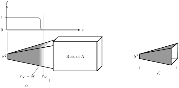
Figure 1: (left) Localization function on $X$ allowing a local study of the heat trace asymptotics; (right) Sharp cut-off at finite radius.

In practice, we however avoid dealing with a “fuzzy boundary” by declaring $\hat{C}$ to be the resolved conifold sharply truncated at $r=r_{\infty}$ (fig. 1, right). From now on, we deal with the heat trace $Z_{\hat{C}}(t,\epsilon)={\rm Tr}_{\hat{C}}e^{-t\Delta}$ on this space. Following (4.6), we address the prospect of bounding $Z_{\hat{C}}(t_{*},\epsilon)$ independently of $\epsilon$ in the limit $\epsilon\to 0$ for $t_{*}$ fixed but small.

5.3 Asymptotics on the resolved conifold

A side-effect of the cut-off is to generate spurious heat trace boundary contributions, which are ultimately of no interest. Assuming Dirichlet boundary conditions (a choice to which we will stick all along), the leading of these terms is a negative contribution:

$$a_{1}^{\partial\hat{C}}(1)=-\frac{\sqrt{\pi}}{216}r_{\infty}^{5}\sqrt{\left(1+\frac{6\epsilon^{2}}{r_{\infty}^{2}}\right)\left(1+\frac{9\epsilon^{2}}{r_{\infty}^{2}}\right)}.$$ (5.10)

However, the now well-posed geometry (sharply truncated) only differs superficially from the smoother one excised from $X$, so we expect bulk spectral behaviour to be the same. Except now, (5.2)–(5.5) can be conveniently used to calculate explicitly $a_{2n}^{\hat{C}}(1)$, $n=0,1,\ldots$ These are the bulk contributions attributable to the resolved conifold-like patch in the heat trace expansion on (the more untractable space) $X$. We have calculated them exactly up to order $6$:

$$a_{0}^{\hat{C}}(1) =\frac{r_{\infty}^{6}}{648}\left(1+\frac{9\epsilon^{2}}{r_{\infty}^{2}}\right)$$ (5.11)

$$a_{2}^{\hat{C}}(1) =0$$ (5.12)

$$a_{4}^{\hat{C}}(1) =\frac{r_{\infty}^{2}}{810}\left(1+\frac{6\epsilon^{2}}{r_{\infty}^{2}}\right)^{-4}\left(2+\frac{45\epsilon^{2}}{r_{\infty}^{2}}+\frac{360\epsilon^{4}}{r_{\infty}^{4}}+\frac{1080\epsilon^{6}}{r_{\infty}^{6}}\right)$$ (5.13)

$$a_{6}^{\hat{C}}(1) =\frac{1}{8505}\ln\left(1+\frac{r_{\infty}^{2}}{6\epsilon^{2}}\right)-\frac{1}{99225}\left(1+\frac{6\epsilon^{2}}{r_{\infty}^{2}}\right)^{-7}\left(284+\frac{11963\epsilon^{2}}{r_{\infty}^{2}}+\frac{214564\epsilon^{4}}{r_{\infty}^{4}}\right.$$

$$\qquad\left.+\frac{2127300\epsilon^{6}}{r_{\infty}^{6}}+\frac{12594960\epsilon^{8}}{r_{\infty}^{8}}+\frac{35789040\epsilon^{10}}{r_{\infty}^{10}}+\frac{544320\epsilon^{12}}{\epsilon^{12}}\right)$$ (5.14)

The dominant term $a_{0}^{\hat{C}}(1)$ is proportional to $\mathop{\rm vol}\hat{C}$; a consequence of Weyl’s law (4.4) applied here to $\hat{C}$ rather than $X$. The effect of the parameter $\hat{R}=(\mathop{\rm vol}\hat{C})^{1/6}$ was previously addressed above, so we might want to fix it in order to focus on the intrinsic effect of changing the radius of the $S^{2}$. More conveniently, we will allow it to vary continuously as $\epsilon\to 0$ and absorb the change of volume in $X\backslash U$ in such a way that $\mathop{\rm vol}X=1$ is constant all the way in the limit. The sub-leading term $a_{2}^{\hat{C}}(1)$ vanishes by virtue of Ricci-flatness, so the first non-trivial signature of finite $\epsilon$ emerges at order 4. It is noteworthy that $a_{4}^{\hat{C}}(1)$ is positive and bounded in the limit $\epsilon\to 0$.

The next term $a_{6}^{\hat{C}}(1)$ however starts exhibiting logarithmic divergence. A simple argument suggests the leading divergence as $\epsilon\to 0$ at higher orders. On the vanishing $S^{2}$ at $r=0$, the curvature behaves as $R\sim 1/\epsilon^{2}$. The curvature enters $a_{2k}^{\hat{C}}(1)$ through its $k$-th power, thus yielding a $\sim\epsilon^{-2k}$ behaviour. Finally, the volume integral contributes an extra shift of the power by the dimension:

$$a_{2k}^{\hat{C}}(1)\sim\epsilon^{6-2k},\qquad(k>3).$$ (5.15)

These remarks seemingly imply that, no matter how small we make $t_{*}$, as $\epsilon$ approaches $0$, $Z_{\hat{C}}(t_{*},\epsilon)$ will grow without bounds. If this were the case, we would at the least need to stay clear of any conifold singularities in the moduli space in order to obtain a bound of the type (4.6). For a single localized singularity such as on $\hat{C}$, this can be achieved by simply making the resolution parameter large enough. However, in the presence of numerous shrinkable 2- and 3-cycles in the complete manifold $X$, avoiding the formation of all the potential singularities could prevent the bound from being uniform in the topology of $X$.

On the other hand, the expansion itself is only guaranteed to be valid for fixed geometry and $t\to 0$. The question we have asked instead concerns the limit $\epsilon\to 0$ for small (but fixed) $t$. It is possible that $Z_{\hat{C}}(t,\epsilon)$, thought of as a function $\mathbb{R}_{\epsilon}^{+}\times\mathbb{R}_{\sqrt{t}}^{+}\to\mathbb{R}^{+}$, does not admit a joint expansion in ($\epsilon$,$\sqrt{t}$), but that it is still bounded despite what the expansion in one of the variables might lead us to suppose. Indeed, the general mathematical expectation (see for instance, [19]) is that the trace of the heat kernel is well-behaved on the (real) blow up of $\mathbb{R}_{\epsilon}^{+}\times\mathbb{R}_{\sqrt{t}}^{+}$ (fig. 2) at the origin. Proving such claims however involves dwelling into the realm of microlocal analysis (see in particular Melrose [20, 21]). An alternative route, described in the next section, is to take advantage of our explicit metric to examine the spectral properties of $\hat{C}$. This approach already provides compelling evidence for the existence of a bound, as we shall see.

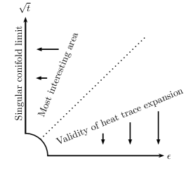
Figure 2: Domain of $Z_{\hat{C}}(t,\epsilon)$ blown up at the origin

5.4 Asymptotics on spaces with conical singularities

Let us close this section by pointing out that the analysis of the heat trace can be carried out as well on the singular conifold $C$ (i.e., in the limit $\epsilon=0$ itself). The question of whether the heat trace displays any kind of divergence as $\epsilon\to 0$ can then be reformulated as a question of continuity in the same limit.

The heat trace asymptotics on spaces with conical singularities was studied by Cheeger [22]. The first step of the analysis is to ensure that the eigenvalue problem is well-defined on the singular space. For the scalar problem, this can easily be verified by separation of variables and reduction to a one-dimensional problem, which we will study in the next section. Quite similarly, one can analyze the Laplacian on forms of arbitrary degree on a space with conical singularities. One finds that this operator is essentially self-adjoint (so the eigenvalue problem is well-defined by itself) unless the base of the cone has non-trivial middle-dimensional cohomology (in which case a choice of boundary condition at the singularity is required to make the problem well-defined).

Cheeger then showed that the heat trace (for forms of arbitrary degree) on a manifold with conical singularities admits an asymptotic expansion very similar in essence to (5.1) (see also [23] for an application to metric cones). Some of the terms of this expansion can be thought of as the above (5.2)–(5.5) having been “regulated” in order to tame the contribution from the infinite curvature at the tip. More precisely, a $u$-sized conical patch is removed from the manifold (much like we did in subsection 5.2) and the integrals in (5.2)–(5.5) are taken over the remaining space. In the limit $u\to 0$, the integrals do not converge but the infinite term can be unambiguously identified and subtracted. The finite part that is left is what enters the asymptotic expansion on the singular manifold. It is noteworthy that the infinite parts diverge as $\ln(u)$ (for $n=d$, where $d$ is the real dimension of the manifold) and $u^{d-k}$ (for $n>d$). This is strongly reminiscent of our situation (cf. (5.14),(5.15)).

We have not tried to make more precise the intuition that the finite parts in (5.11)–(5.14) are the relevant ones for the heat trace expansion in the singular limit $\epsilon=0$. However, the existence of the expansion at $\epsilon=0$ together with the general expectation mentioned above, is reasonable evidence that the divergence of the coefficients is merely an artifact of the asymptotic expansion for $t\to 0$ at fixed $\epsilon$, whereas the full heat trace can still be continuous in the limit $\epsilon\to 0$ for finite $t$. If this is the case, the asymptotic expansion on the singular manifold would be a useful starting point for estimating $Z_{\hat{C}}(t,\epsilon)$ on the resolution. With a resolution of order $1/R_{*}$, this estimate could be useful to establish a bound of the form (4.6) on $Z_{X}(t)$ for the complete manifold $X$.

An alternative argument against the persistence of the divergences goes as follows. In the degenerate case $\epsilon=0$, additional contributions to the $t$-independent terms and extra $\sim\ln t$ terms need to be added to the heat trace expansion (5.1) [22]. There is thus a qualitative discontinuity in the nature of the two expansions. The infinities might thus reflect the fact that the expansion ceases to be a valid representation of $Z_{\hat{C}}(t,\epsilon)$, rather than indicating a divergence in the heat trace itself. If the transition is indeed continuous, the infinities coming from the expansion at finite $\epsilon$ must conspire (through some re-summation of the divergent asymptotic series) to yield the logarithms and additional terms in the expansion for $\epsilon=0$.

6 Exact Spectral Analysis on Conifolds

Given the limitations of the asymptotic approach, we now consider more closely the spectrum of the scalar Laplacian on $\hat{C}$. The question of boundedness of $Z_{\hat{C}}(t,\epsilon)$ in the limit $\epsilon\to 0$ can be recast in a question about the behaviour of the eigenvalues in the same limit. Let us denote $N_{\hat{C}}(\lambda,\epsilon)$ the number of eigenvalues of $\Delta$ smaller than $\lambda$. We will call it the (full) counting function of the eigenvalues. Suppose it is bounded above (for $\epsilon$ small enough) by some function $B(\lambda)$ independent of $\epsilon$. Then the fact that $Z_{\hat{C}}(t,\epsilon)$ is the Laplace transform of the derivative of $N_{\hat{C}}(\lambda,\epsilon)$ with respect to $\lambda$ entails readily an upper bound on the heat trace itself. In terms of the individual eigenvalues, bounding the counting function is equivalent to having only finitely many eigenvalues dropping below any fixed (large enough) $\lambda$ as $\epsilon\to 0$.

In this section, we provide an analytical analysis of the eigenvalue problem and discuss its ramifications and limitations. In section 7, we come back to it using high-order WKB expansions. This approach and the above formulation in terms of $N_{\hat{C}}(\lambda,\epsilon)$ allow us to finally claim a positive answer to the question raised at the end of section 5.2.

6.1 Singular conifold

An advantage of considering first the singular conifold is that the eigenvalue problem of the scalar Laplacian on this space is completely amenable to separation of variables. Its solution, which we now briefly review, offers a benchmark to refer to when analyzing spaces resolving the singularity.

Upon setting $\epsilon=0$ in (5.8), $\hat{C}$ becomes manifestly the metric cone $C$ over $T^{1,1}$ (still truncated at a finite $r=r_{\infty}$). For cones, the eigenvalue problem splits into a “radial” differential equation, which determines the spectrum, and an eigenvalue problem on the base space. Letting the eigenfunctions be denoted

$$f^{n,m,l_{1},m_{1},l_{2},m_{2}}(r,\psi,\theta_{1},\phi_{1},\theta_{2},\phi_{2})=\text{R}^{n,m,l_{1},l_{2}}(r)\Psi^{m}(\psi)\prod_{k=1}^{2}\Theta_{k}^{m,l_{k},m_{k}}(\theta_{k})\Phi_{k}^{m_{k}}(\phi_{k}),$$ (6.1)

the radial equation,

$$\frac{1}{r^{5}}\frac{d}{dr}\left(r^{5}\frac{d}{dr}\text{R}^{m,l_{1},l_{2}}(r)\right)+\left(\lambda-\frac{\Lambda^{m,l_{1},l_{2}}}{r^{2}}\right)\text{R}^{m,l_{1},l_{2}}(r)=0,$$ (6.2)

is Bessel differential equation (up to the change of variable $r\to\sqrt{\lambda}r$ ($\lambda\neq 0$) and factorizing $(\sqrt{\lambda}r)^{-2}$ out of $\text{R}^{m,l_{1},l_{2}}(r)$). Requiring the eigenfunctions to be regular on $[0,r_{\infty}]$ and Dirichlet boundary condition at $r=r_{\infty}$ picks out the solution of the first kind

$$\text{R}^{m,l_{1},l_{2}}(r)\propto\frac{1}{\lambda r^{2}}J_{\sqrt{\Lambda^{m,l_{1},l_{2}}+4}}(\sqrt{\lambda}r).$$ (6.3)

The spectrum is determined from the strictly positive zeros of the Bessel function:

$$J_{\sqrt{\Lambda^{m,l_{1},l_{2}}+4}}(\sqrt{\lambda}r_{\infty})=0.$$ (6.4)

Here $\Lambda^{m,l_{1},l_{2}}$ are Laplacian eigenvalues on the base manifold $T^{1,1}$. Along with the eigenfunctions, they have been worked out in [18, 24, 25]:

$$\Lambda^{m,l_{1},l_{2}}=9m^{2}+\sum_{k=1}^{2}\Lambda_{k}^{m,l_{k}},\quad\Lambda_{k}^{m,l_{k}}=6[l_{k}(l_{k}+1)-m^{2}],$$ (6.5)

$$\Psi^{m}(\psi)=e^{im},\quad m\in\{-\min(l_{1},l_{2}),...,+\min(l_{1},l_{2})\}\text{ (integer increments)}$$ (6.6)

$$\Phi_{k}^{m_{k}}(\phi_{k})=e^{im_{k}},\quad m_{k}\in\{-l_{k},...,+l_{k}\}\text{ (integer increments)}$$ (6.7)

$$\Theta_{k}^{m,l_{k},m_{k}}(\theta_{k})=\left\{\begin{array}[]{l l}\sin^{m_{k}}\theta_{k}\cot^{m}\frac{\theta_{k}}{2}{}_{2}F_{1}({\scriptstyle-l+m_{k}},{\scriptstyle 1+l+m_{k}},{\scriptstyle 1+m_{k}-m_{~{}}},\sin^{2}\frac{\theta_{k}}{2})&m_{k}\geq m\\ \sin^{m}\theta_{k}\cot^{m_{k}}\frac{\theta_{k}}{2}{}_{2}F_{1}({\scriptstyle-l+m_{~{}}},{\scriptstyle 1+l+m_{~{}}},{\scriptstyle 1+m_{~{}}-m_{k}},\sin^{2}\frac{\theta_{k}}{2})&m_{k}\leq m\end{array}\right.$$ (6.8)

with either both $l_{k}\in\{0,1,2,...\}$ or both $l_{k}\in\{\frac{1}{2},\frac{3}{2},\frac{5}{2},...\}$, $k=1,2$.

Note that harmonic functions, corresponding to $\lambda=0$, are irrelevant here since the only solutions to $\Delta f=0$ (being thought of as the steady state source-free heat equation) are constant functions over $C$. The Dirichlet condition at the cut-off then picks up $f=0$, which has to be discarded.

6.2 Resolved conifold

Since the resolved and singular conifolds share the same $SU(2)_{l_{1},m_{1}}\times SU(2)_{l_{2},m_{2}}\times U(1)_{m}$ symmetry (at the level of the algebra), the eigenvalue problem on $\hat{C}$ is structurally identical to the above. Separation of variables yields again a complete solution and, in fact, the “angular” parts of the eigenfunctions remain unchanged (i.e., (6.5)–(6.8) are still valid). Moreover, the spectrum information is still encoded in a radial ordinary differential equation. It takes the form

$$\frac{1}{r^{3}(r^{2}+6\epsilon^{2})}\frac{d}{dr}\left(r^{3}(r^{2}+9\epsilon^{2})\frac{d}{dr}\text{R}^{m,l_{1},l_{2}}(r,\epsilon)\right)+\left(\lambda-\frac{\Lambda^{m,l_{1},l_{2}}(r,\epsilon)}{r^{2}}\right)\text{R}^{m,l_{1},l_{2}}(r,\epsilon)=0$$ (6.9)

where

$$\frac{\Lambda^{m,l_{1},l_{2}}(r,\epsilon)}{r^{2}}=\frac{\Lambda_{1}^{m,l_{1}}}{r^{2}}+\frac{\Lambda_{2}^{m,l_{2}}}{r^{2}+6\epsilon^{2}}+\frac{9m^{2}}{r^{2}}\frac{r^{2}+6\epsilon^{2}}{r^{2}+9\epsilon^{2}}.$$ (6.10)

Before exhibiting the exact solution to this differential equation, let us study certain limit cases. For $r\gg\epsilon$, the equation reduces to (6.2), so the general asymptotic solution is

$$\text{R}^{m,l_{1},l_{2}}(r,\epsilon)\sim\frac{c_{1}}{r^{2}}J_{\sqrt{\Lambda^{m,l_{1},l_{2}}+4}}(\sqrt{\lambda}r)+\frac{c_{2}}{r^{2}}Y_{\sqrt{\Lambda^{m,l_{1},l_{2}}+4}}(\sqrt{\lambda}r)\qquad(r\gg\epsilon),$$ (6.11)

just like in the singular case. For $r\ll\epsilon$, (6.9) is also a Bessel equation, but the eigenvalues get shifted and the effective dimension of the base changes from $5$ to $3$. The normalizable solution at $r=0$ is

$$\text{R}^{m,l_{1},l_{2}}(r,\epsilon)\sim\frac{1}{r}J_{\sqrt{\frac{2}{3}\Lambda_{1}^{m,l_{1}}+4m^{2}+1}}\bigg{(}\sqrt{\frac{2}{3}\lambda-\frac{\Lambda_{2}}{9\epsilon^{2}}}r\bigg{)}\qquad(r\ll\epsilon).$$ (6.12)

The complexity of our problem lies in understanding how to choose $c_{1},c_{2}$ (both real functions of $\epsilon,\lambda,l_{1},l_{2},m$) to patch up the two limiting behaviours. The solution for large $r$ eventually determines the spectrum upon evaluation at $r=r_{\infty}\gg\epsilon$ and it is not problematic in the limit $\epsilon\to 0$. However, the solution for small $r$ has $\epsilon$ in the denominator. One might thus suspect that the appropriate linear combination (i.e., the constants $c_{1},c_{2}$) behaves uncontrollably in the limit. On the other hand, the validity range of the latter expansion is of shrinking size as $\epsilon\to 0$, so we cannot really progress much further with this approach.

To get a broader picture, we now examine the exact solution of (6.9) by recasting the equation in terms of some new independent and dependent variables:

$$r\to x=-\frac{r^{2}}{9\epsilon^{2}}$$ (6.13)

$$\text{R}^{m,l_{1},l_{2}}(r,\epsilon)=x^{\frac{1}{2}\sqrt{\frac{2}{3}\Lambda_{1}^{m,l_{1}}+4m^{2}+1}-\frac{1}{2}}(1-x)^{m/2}H^{m,l_{1},l_{2}}(x,\epsilon).$$ (6.14)

The multiplicative function we have inserted in (6.14) is non-vanishing on $[-\frac{r_{\infty}^{2}}{9\epsilon^{2}},0)$ and regular on the closure of this interval, which is the domain of $H^{m,l_{1},l_{2}}(x,\epsilon)$. This function then still contains the full information about the spectrum. Substituting (6.13)–(6.14) in (6.9) yields

$$\frac{d^{2}H^{m,l_{1},l_{2}}(x,\epsilon)}{dx^{2}}+\left(\frac{\gamma^{m,l_{1}}}{x}+\frac{\delta^{m}}{x-1}-\beta\right)\frac{dH^{m,l_{1},l_{2}}(x,\epsilon)}{dx}-\frac{\alpha(\epsilon)x-q^{m,l_{1},l_{2}}(\epsilon)}{x(x-1)}H^{m,l_{1},l_{2}}(x,\epsilon)=0$$ (6.15)

where we have set

$$\alpha(\epsilon) =\frac{9\epsilon^{2}\lambda}{4},$$ (6.16)

$$\beta =0$$ (6.17)

$$\gamma^{m,l_{1}} =1+\sqrt{\frac{2}{3}\Lambda_{1}^{m,l_{1}}+4m^{2}+1}$$ (6.18)

$$\delta^{m} =m+1$$ (6.19)

$$q^{m,l_{1},l_{2}}(\epsilon) =\frac{3\epsilon^{2}\lambda}{2}+\frac{(m+1)}{2}\bigg{(}1+\sqrt{\frac{2}{3}\Lambda_{1}^{m,l_{1}}+4m^{2}+1}\bigg{)}-\frac{\Lambda_{1}^{m,l_{1}}}{12}-\frac{\Lambda_{2}^{m,l_{2}}}{4}-m^{2}-1$$ (6.20)

Eq. (6.15) is a standard form of the confluent Heun equation [26], a degenerate version of the generic second order equation with four regular singular points (at $x=0,1,a,\infty$). It is obtained from the general Heun equation by a “confluence process” (described e.g. in [27]), which merges the singularity at $x=a$ with that at $x=\infty$. This results in a rank-2 irregular singular point at infinity and leaves behind the finite regular singular points at $0$ and $1$. We will call $\text{HeunC}(\alpha,\beta,\gamma,\delta,q;x)$ the solution of (6.15) finite at $x=0$. It is normalized with the condition $\text{HeunC}(\alpha,\beta,\gamma,\delta,q;0)=1$. One can easily check that the $r\to 0$ behaviour of $\text{R}^{m,l_{1},l_{2}}(r,\epsilon)$ (cf. (6.14)) matches that derived from (6.12).

The connection between Heun equation and the resolved conifold comes with a light sense of déjà vu, as it occurred in related eigenvalue problems. For instance, Oota and Yasui [28] have exhibited its role in the spectrum of some five-dimensional toric Sasaki-Einstein manifolds (which include $T^{1,1}$ as a particular case). Eq. (6.15) also comes about in the Laplacian eigenvalue problem on the Eguchi-Hanson space [29]. This space can be thought of as a resolution of a singularity on Calabi-Yau twofolds.

Further confluent cases of Heun equation can be obtained from (6.15), yielding so-called double-confluent, biconfluent, and triconfluent Heun equations. One might anticipate that solutions to confluent versions of an equation can be obtained as limit cases of solutions to the original equation. Although this is possible, one should worry about possible qualitative discrepancies due to the various different ways in which the two points can approach each other [27]. For some cases, the spectra defined by the equations may be continuous [30]; for others, drastic non-analytic changes can be expected [31, 32].

These remarks take a critical importance regarding the question of convergence of the resolved conifold spectrum to that of the singular conifold. Indeed, the limit $\epsilon\to 0$ that we are interested in corresponds to yet another confluence process now taking the singular point at $1$ to that at $0$. This is better seen in terms of the variable $y=r^{2}=-9\epsilon^{2}x$:

$$\frac{d^{2}H(y)}{dy^{2}}+\left(\frac{\gamma}{y}+\frac{\delta}{y+9\epsilon^{2}}+9\epsilon^{2}\beta\right)\frac{dH(y)}{dy}+\frac{\lambda y/4+q}{y(y+9\epsilon^{2})}H(y)=0$$ (6.21)

(dropping explicit labels). The singular points of this equation on the punctured Riemann sphere are pictured on fig. 3 (left), while fig. 3 (right) shows those for $\epsilon=0$.

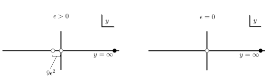
Figure 3: Regular ($\circ$) and irregular ($\bullet$) singular points of (6.21) in $\mathbb{C}_{y}$ for $\epsilon>0$ (left) and $\epsilon=0$ (right).

The question whether the confluence process occurring here causes uncontrolled behaviour or not is much more delicate than it seems a priori, as discussed in the literature afore-cited. Also, the most readily available asymptotic expansions of confluent Heun solutions are ill-suited to study the connection between (6.11) and (6.12) usefully. However, numerical tests strongly suggest that the transition

$$\frac{1}{r^{2}}J_{\sqrt{4+\Lambda^{m,l_{1}}}}(\sqrt{\lambda}r)\to\frac{1}{r^{2-\gamma^{m,l_{1}}}}(r^{2}+9\epsilon^{2})^{m/2}\text{HeunC}\Big{(}\alpha(\epsilon),0,\gamma^{m,l_{1}},\delta^{m},q^{m,l_{1},l_{2}}(\epsilon);-\frac{r^{2}}{9\epsilon^{2}}\Big{)}$$ (6.22)

undergone by the eigenfunction upon resolution of the singularity is continuous and sufficiently well behaved for the heat trace to be bounded in the limit $\epsilon\to 0$. We give, in the following section, an argument based on the full WKB expansion of (6.9).

7 Full WKB Expansions of Radial Counting Functions

Our argument is essentially the Bohr-Sommerfeld approximative quantization rule treated with some extra care. We thus need to recast the radial eigenvalue problem as a Schrödinger equation. Again, as a warm-up, we consider the singular case first.

In this section, we take advantage of our knowledge that the eigenvalues we are interested in arise from a collection of 1-d boundary value problems. In particular, instead of considering the full counting function

$$N_{\hat{C}}(\lambda,\epsilon)=\sum_{l_{1},l_{2},m}n_{l_{1},l_{2},m}(\lambda,\epsilon),$$ (7.1)

we focus on the individual functions $n_{l_{1},l_{2},m}(\lambda,\epsilon)$, which count the number of eigenvalues—with $l_{1},l_{2},m$ fixed—below $\lambda$. The sum is finite for any fixed value of $\lambda$ and the number of elements it contains is essentially bounded above by the volume in the space of quantum numbers, i.e., by Weyl’s law. We can thus concentrate on bounding each $n_{l_{1},l_{2},m}(\lambda,\epsilon)$ independently.

7.1 Singular conifold

Upon setting

$$\psi(r)=\psi^{m,l_{1},l_{2}}(r)=r^{5/2}\text{R}^{m,l_{1},l_{2}}(r),$$ (7.2)

eq. (6.2) becomes a Schrödinger equation:

$$\hbar^{2}\frac{d^{2}}{dz^{2}}\psi(z)=Q(z)\psi(z),\qquad Q(z)=V(z)-\lambda,$$ (7.3)

with $z=r$, $\hbar=1$, and the following radial confining potential:

$$V(z)=V^{m,l_{1},l_{2}}(z,0)=\begin{cases}\frac{1}{z^{2}}\left(\Lambda^{m,l_{1},l_{2}}+\frac{15}{4}\right)&0\leq z\leq r_{\infty}\\ \infty&\text{else.}\end{cases}$$ (7.4)

The WKB approximation to the bound states is obtained from the ansatz

$$\psi(z)=\exp\left[\frac{1}{\hbar}\sum_{k=0}^{\infty}\hbar^{k}S_{k}(z)\right]$$ (7.5)

by keeping only the first two terms in the series. Its validity increases as $\hbar\to 0$ or, for fixed $\hbar$ as $\lambda\to\infty$ [34]. The approximation is typically very precise on the whole range of the independent variable, except near the two turning points, defined by the condition $Q(z)=0$. Plugging (7.5) into the Schrödinger equation yields

$$S_{0}^{\prime}(z) =\pm\sqrt{Q(z)}$$ (7.6)

$$S_{1}^{\prime}(z) =-\frac{1}{4}\ln Q(z).$$ (7.7)

Careful matching of the oscillatory behaviour in the region where $\lambda>V(z)$ (i.e., $Q(z)<0$) with the exponential decay in the classically forbidden regions (beyond the turning points) yields the celebrated Bohr-Sommerfeld energy quantization rule:

$$\left(n+\frac{1}{2}\right)\hbar\pi\approx\int\sqrt{-Q(z)}dz,\qquad(n=0,1,2,\ldots).$$ (7.8)

The integral is taken from the smallest to the largest turning points.

Changing viewpoint, we can regard (7.8) as an approximation to the individual counting functions introduced above. In the case of the singular conifold, this expression is found to describe very accurately the distribution of the zeros of the Bessel function. Carrying out the integral, with the potential (7.4), gives

$$n_{l_{1},l_{2},m}(\lambda,0)\approx\frac{\sqrt{\mu^{2}-1/4}}{\pi}\left[\sqrt{\frac{\lambda r_{\infty}^{2}}{\mu^{2}-1/4}-1}-\arccos\left(\sqrt{\frac{\mu^{2}-1/4}{\lambda r_{\infty}^{2}}}\right)\right]-\frac{3}{4},$$ (7.9)

where $\mu=\sqrt{\Lambda^{m,l_{1},l_{2}}+4}$ is the order of the Bessel function giving rise to the spectrum. As a consistency check, it is possible to obtain precisely Weyl’s law for any metric cone, with all proportionality factors, from this formula (assuming only that the law holds on the base manifold) cf. appendix A. Ref. [35] also used a minor variant of this formula to obtain the second term of the expansion in the case of the 2-dimensional disc.

7.2 Resolved conifold

In the case of the resolved conifold, eq. (6.9) becomes a Schrödinger equation at the expense of a complicated change of variable necessary to remove the factor multiplying the eigenvalues:

$$r\to z=-i\sqrt{6}\epsilon\text{E}\Big{(}\frac{ir}{3\epsilon},\frac{\sqrt{6}}{2}\Big{)}.$$ (7.10)

It arises from the property

$$\frac{dz}{dr}=\sqrt{\frac{r^{2}+6\epsilon^{2}}{r^{2}+9\epsilon^{2}}}.$$ (7.11)

Here $\text{E}(x,k)$ denotes the incomplete elliptic integral of the second kind. Following this change of variable, we must substitute the dependent variable as

$$\psi(z)=\psi^{m,l_{1},l_{2}}(z,\epsilon)=\sqrt{r^{3}\sqrt{(r^{2}+6\epsilon^{2})(r^{2}+9\epsilon^{2})}}\text{R}^{m,l_{1},l_{2}}(z,\epsilon)$$ (7.12)

to obtain an equation in the form (7.3). The effective potential energy is conveniently written in terms of $r$, which should now be regarded as a function of $z$:

$$V^{m,l_{1},l_{2}}(z,\epsilon)=\frac{\Lambda^{m,l_{1},l_{2}}(r,\epsilon)}{r^{2}}+\frac{15r^{8}/4+90r^{6}\epsilon^{2}+765r^{4}\epsilon^{4}+2592r^{2}\epsilon^{6}+2187\epsilon^{8}}{r^{2}(r^{2}+6\epsilon^{2})^{2}(r^{2}+9\epsilon^{2})^{2}}\left(\frac{dz}{dr}\right)^{-2}.$$ (7.13)

(Of course, the potential is again infinite outside the range $0\leq r<r_{\infty}$.)

In the present case, the Bohr-Sommerfeld integral cannot be performed exactly as previously. We observe instead that the potential function reduces to (7.4) for $\epsilon=0$ (thus the choice of notations). Hence, the left turning point of the resolved problem limits to that of the singular problem, that is $\sqrt{(\Lambda^{m,l_{1},l_{2}}+15/4)/\lambda}$, when $\epsilon\to 0$. Since this is always strictly positive (albeit small), no divergence can be due to evaluation of (7.8) at the turning points. This holds regardless of the value of $\epsilon$.

If any discontinuity occurs in the confluence process, we should thus see its effects in the integrand only. Nothing of this kind occurs in the leading Bohr term as can be seen easily from the potential function (7.13). However, given the asymptotic analysis done on the heat trace in section 5, we could expect negative powers of $\epsilon$ to arise at higher orders.

Let us then consider the full formal solution of Schrödinger equation in terms of the WKB ansatz (7.5). The next terms after (7.6) can be obtained recursively from [34]

$$2S^{\prime}_{0}(z)S^{\prime}_{k}+S^{\prime\prime}_{k-1}(z)+\sum_{j=1}^{k-1}S^{\prime}_{j}S^{\prime}_{k-j}=0,\qquad(k=2,3,4,\ldots).$$ (7.14)

The leading of these corrections are

$$S^{\prime}_{2}(z) =\pm\left[\frac{Q^{\prime\prime}(z)}{8Q(z)^{3/2}}-\frac{5(Q^{\prime}(z))^{2}}{32Q(z)^{5/2}}\right],$$ (7.15)

$$S^{\prime}_{3}(z) =-\frac{Q^{\prime\prime}(z)}{16Q^{2}(z)}+\frac{5(Q^{\prime}(z))^{2}}{64Q^{3}(z)},$$ (7.16)

$$S^{\prime}_{4}(z) =\pm\left[\frac{Q^{\prime\prime\prime\prime}}{32Q^{5/2}}-\frac{7Q^{\prime}Q^{\prime\prime\prime}}{32Q^{7/2}}-\frac{19(Q^{\prime\prime})^{2}}{128Q^{7/2}}+\frac{221Q^{\prime\prime}(Q^{\prime})^{2}}{256Q^{9/2}}-\frac{1105(Q^{\prime})^{4}}{2048Q^{11/2}}\right].$$ (7.17)

It is easy to convince oneself that the structure of these expressions is qualitatively the same at any order: sums of ratios of derivatives of the shifted potential $Q(z)$ to powers of $Q(z)$. It is a known fact that odd terms are total derivatives and single-valued. The even terms all involve square roots of $Q(z)$. Thought of as complex functions, they have two branches (thus the $\pm$ signs). [34]

The two independent solutions obtained by summing all these terms are exact but generally divergent on the whole complex $z$ plane. They must be interpreted as asymptotic expansions of the true solutions. The Bohr-Sommerfeld rule is consequently understood as the first term of the full WKB expansion [36, 34]

$$\left(n+\frac{1}{2}\right)\sim\frac{1}{2\pi i}\oint\frac{1}{\hbar}\sum_{j=0}^{\infty}\hbar^{2j}S^{\prime}_{2j}(z)dz,\qquad\lambda\to\infty.$$ (7.18)

The contour encircles the two turning points, and no other singularity in the complex $z$ plane. The sign of the $S^{\prime}_{2j}(z)$ must be adjusted so that the integral is performed on a smooth branch whose cut connects the turning points on the real axis.

We now make our argument on boundedness of the counting functions $n_{l_{1},l_{2},m}(\lambda,\epsilon)$ and thus, by our previous discussion, of $Z_{\hat{C}}(t,\epsilon)$. We again identify $n$ in (7.18) as an individual counting function (corresponding to the quantum numbers $l_{1},l_{2},m$).

Unlike the Minakshisundaram-Pleijel heat trace expansion (cf. (5.1)), the full WKB expansion does not exhibit any divergence in the limit $\epsilon\to 0$. This can be seen after close inspection of (7.14), (7.13) and (7.11), and indicates that the singular space heat trace $Z_{C}(t)=Z_{\hat{C}}(t,0)$ can be used as a starting point to bound $Z_{\hat{C}}(t,\epsilon)$.

One may reasonably ask why we should trust the continuity of the WKB expansion more than the divergence of the heat trace expansion? As was discussed in section 5, the latter expansion is in fact ill-suited to our discussion as it is valid for $t\to 0$ and $\epsilon$ fixed, while we need the opposite regime. Also, and this is the key remark, its qualitative form changes discontinuously when $\epsilon=0$ (cf. subsection 5.4). This is not the case for the WKB expansion. Indeed, we saw in subsection 7.1 that WKB ideas can be usefully exploited to solve non-trivial questions even in the singular case. The qualitative form of the expansion is insensitive to the existence (or not) of a singularity. We conclude therefore that the conclusions drawn from (7.18) are in fact correct, and maintain that $Z_{\hat{C}}(t_{*},\epsilon)$ can be bounded above independently of $\epsilon$ in the limit $\epsilon\to 0$.

8 Discussion

We have argued in the previous section that the spectrum of the scalar Laplacian on the resolved conifold is continuous in the singular limit, as expected on general mathematical grounds. The main step in the argument is based on the analysis of the 1-dimensional radial Schrödinger equation that results after separation of variables. The divergence of the asymptotic expansion of the trace of the heat kernel is a remnant of the breakdown of the classical propagation across the singularity, while the quantum mechanical evolution is well-behaved at finite energy. This confirmation of physical intuition makes us confident that analogous statements should hold for more general singularities as well. An obvious next test case would be the deformed conifold, on which the wave equation is not reducible to a purely one-dimensional problem because of the smaller symmetry algebra.

We now wish to discuss the lessons for the question (4.6) that we proposed as a geometric supplement to the SCHOK bound (2.4) on the number of marginal deformations of a conformal field theory.

Since we are allowed to move around in the moduli space of Ricci-flat metrics, we can imagine approaching the question by speculating that a general compact Calabi-Yau manifold of complicated topology can, by deformation of the metric, be decomposed into flatter regions that are connected and/or terminated by regions of concentrated curvature, intuitively similar to what is possible for Riemann surfaces. The question is then whether the contribution to the heat trace from the curved regions can be estimated and bounded in a uniform fashion.

Now, had it turned out that the heat trace were in fact not continuous at the approach of a singularity, we would have had to stay at a finite distance from all singularities in the moduli space of metrics. Since we expect the number of singularities to increase with the dimension of the moduli space, it would be very delicate to find a region in which to bound the heat trace in very high-dimensional moduli spaces, and any resulting bound would unlikely be uniform.

Under the hypothesis of spectral continuity however, curvature singularities (at least those of the type we analyzed) do not in fact preclude a bound on the heat trace. On the contrary, if the manifold can in fact be simplified in the way described above, the singular limit could prove a useful starting point from which to estimate the heat trace on the smooth manifold. This has a chance of being uniform in the topology and the string scale.

Acknowledgments We thank Simeon Hellerman for asking the question which led to this research, as well as for collaboration at an initial stage. We would like to thank Dmitry Jakobson, Frédéric Rochon, and David Sher for valuable discussions related to the heat kernel expansion. This research was supported by an Alexander Graham Bell Canadian Graduate Scholarship (NSERC), a Bourse de maîtrise en recherche (FRQNT), funds provided by a Tier II Canada Research Chair, and an NSERC Discovery Grant.

Appendix A Weyl’s law for cones from WKB expansion

As an application of formula (7.9), we obtain here Weyl’s law for any $(d+1)$-dimensional metric cone $C_{B}$ over a $d$-dimensional manifold $B$ ($ds_{C_{B}}^{2}=dr^{2}+r^{2}ds_{B}^{2}$). As usual, we assume the cone is truncated at $r=r_{\infty}$. We use only the differential equation: the exact solution in terms of Bessel functions is unnecessary. We also assume that Weyl’s law is satisfied on the base, that is, if $\Lambda$ and $N_{B}(\Lambda)$ are respectively the eigenvalues and the counting function associated with the Laplacian $\Delta_{B}$ on the base, we have

$$N_{B}(\Lambda)\approx\left(\frac{\Lambda}{4\pi}\right)^{d/2}\frac{\mathop{\rm vol}(B)}{\Gamma(d/2+1)},\qquad(\Lambda\to\infty)$$ (A.1)

The goal is to derive this formula with $B$ replaced by $C_{B}$, $\Lambda$ by $\lambda$ (the eigenvalue of the full problem), and $d$ by $d+1$. This form of Weyl’s law is related to (4.4) through a Laplace transformation.

As discussed in the main text (cf. (6.2)), the eigenvalue problem for the Laplacian $\Delta_{C_{B}}$ reduces to the single differential equation

$$\frac{1}{r^{d}}\frac{d}{dr}\left(r^{d}\frac{d}{dr}R(r)\right)+\left(\lambda-\frac{\Lambda}{r^{2}}\right)R(r)=0.$$ (A.2)

The WKB method applied on this equation (rewritten in Schrödinger form) yields the quantization condition (7.9):

$$n\approx\frac{1}{\pi}\left[\sqrt{\lambda r_{\infty}^{2}-\mu^{2}+1/4}-\sqrt{\mu^{2}-1/4}\arccos\left(\sqrt{\frac{\mu^{2}-1/4}{\lambda r_{\infty}^{2}}}\right)\right]-\frac{3}{4}.$$ (A.3)

Here, $\mu=\sqrt{\Lambda+(d-1)^{2}/4}$ is the order of the Bessel equation in which (A.2) can be cast. We can regard this as an implicit expression of $\lambda$ as a function of the radial quantum number $n$ and the base space quantum numbers (encapsulated in $\Lambda$). Fixing a continuous value for $\lambda$, (A.3) can alternatively be regarded as a function of $\Lambda$ delimiting the region of phase space with energies below $\lambda$. To leading order, $N_{C_{B}}(\lambda)$ is then given by the volume of this region:

$$N_{C_{B}}(\lambda)\approx\int n(\Lambda)\big{|}_{\lambda}dN_{B}=\int n(\Lambda)\big{|}_{\lambda}\frac{dN_{B}(\Lambda)}{d\Lambda}d\Lambda.$$ (A.4)

The range of integration is determined as follows. Intuitively, the smallest positive value $\Lambda$ can take is reached when $n(\Lambda)\big{|}_{\lambda}$ is maximal (for fixed $\lambda$). This happens roughly when $\mu^{2}-1/4=0$. Conversely, the upper limit is obtained from the minimal (positive) value of $n(\Lambda)\big{|}_{\lambda}$. It will turn out to be sufficiently precise to consider this to happen when $\mu^{2}-1/4=\lambda r_{\infty}^{2}$.

Defining the integration variable $x=\sqrt{\frac{\mu^{2}-1/4}{\lambda r_{\infty}^{2}}}$, (A.1) gives (to leading order)

$$\frac{dN_{B}(\Lambda)}{d\Lambda}\approx(x\sqrt{\lambda}r_{\infty})^{d-2}\frac{d/2}{(4\pi)^{d/2}}\frac{\mathop{\rm vol}(B)}{\Gamma(d/2+1)}$$ (A.5)

and (A.4) becomes (dropping the shift by $3/4$)

$$N_{C_{B}}(\lambda) \approx\int_{0}^{1}\frac{\sqrt{\lambda}r_{\infty}}{\pi}\left[\sqrt{1-x^{2}}-x\arccos{x}\right](\sqrt{\lambda}r_{\infty})^{d}\frac{d}{(4\pi)^{d/2}}\frac{\mathop{\rm vol}(B)}{\Gamma(d/2+1)}x^{d-1}dx$$

$$=\frac{(\sqrt{\lambda}r_{\infty})^{d+1}}{\pi}\frac{d}{(4\pi)^{d/2}}\frac{\mathop{\rm vol}(B)}{\Gamma(d/2+1)}\int_{0}^{1}\left[\sqrt{1-x^{2}}-x\arccos{x}\right]x^{d-1}dx.$$ (A.6)

We immediately see that the power of $\lambda$ is as expected. The integral can be worked out analytically. It is straightforward to verify from here that the factors match Weyl’s law exactly. The volume arises as $\mathop{\rm vol}(C_{B})=r_{\infty}^{d+1}\mathop{\rm vol}(B)/(d+1)$.

References

- [1] P. Candelas, G. T. Horowitz, A. Strominger and E. Witten, “Vacuum Configurations for Superstrings,” Nucl. Phys. B 258, 46 (1985).
- [2] D. Friedan, E. J. Martinec and S. H. Shenker, “Conformal Invariance, Supersymmetry and String Theory,” Nucl. Phys. B 271, 93 (1986).
- [3] M. Dine and N. Seiberg, “Is the Superstring Weakly Coupled?,” Phys. Lett. B 162, 299 (1985).
- [4] E. Witten, “String theory dynamics in various dimensions,” Nucl. Phys. B 443, 85 (1995) [arXiv:hep-th/9503124].
- [5] S. Kachru, R. Kallosh, A. D. Linde and S. P. Trivedi, “De Sitter vacua in string theory,” Phys. Rev. D 68, 046005 (2003) [arXiv:hep-th/0301240].
- [6] L. Susskind, “The Anthropic landscape of string theory,” In *Carr, Bernard (ed.): Universe or multiverse?* 247-266 [arXiv:hep-th/0302219].
- [7] F. Denef and M. R. Douglas, “Computational complexity of the landscape. I.,” Annals Phys. 322, 1096 (2007) [arXiv:hep-th/0602072].
- [8] S. Hellerman and C. Schmidt-Colinet, “Bounds for State Degeneracies in 2D Conformal Field Theory,” JHEP 1108, 127 (2011) [arXiv:1007.0756 [hep-th]].
- [9] C. A. Keller and H. Ooguri, “Modular Constraints on Calabi-Yau Compactifications,” Commun. Math. Phys. 324, 107 (2013) [arXiv:1209.4649 [hep-th]].
- [10] W. Lerche, C. Vafa and N. P. Warner, “Chiral Rings in N=2 Superconformal Theories,” Nucl. Phys. B 324, 427 (1989).
- [11] S. Hellerman, private communication with J.W.
- [12] P. Candelas and X. C. de la Ossa, “Comments on Conifolds,” Nucl. Phys. B 342, 246 (1990).
- [13] S. Hellerman, “A Universal Inequality for CFT and Quantum Gravity,” JHEP 1108, 130 (2011) [arXiv:0902.2790 [hep-th]].
- [14] P. Gao and M. R. Douglas, “Geodesics on Calabi-Yau manifolds and winding states in nonlinear sigma models,” arXiv:1301.1687 [hep-th].
- [15] P. B. Gilkey, “Asymptotic Formulae in Spectral Geometry,” Chapman & Hall/CRC (2003)
- [16] D. V. Vassilevich, “Heat kernel expansion: user’s manual,” Phys. Rept. 388, 279-360 (2003) [arXiv:hep-th/0306138].
- [17] L. A. Pando Zayas and A. A. Tseytlin, “3-brane on Resolved Conifold,” JHEP 0011:028 (2000) [arXiv:hep-th/0010088].
- [18] I. R. Klebanov and A. Murugan, “Gauge/Gravity Duality and Warped Resolved Conifold,” JHEP 0703:042 (2007) [arXiv:hep-th/0701064].
- [19] R. Mazzeo, “Resolution blowups, spectral convergence and quasi-asymptotically conical spaces,” Journées Équations aux Dérivées Partielles Exposé VIII (2006)
- [20] R. Melrose, “Introduction to Microlocal Analysis,” Online lecture notes: http://www-math.mit.edu/~rbm/iml90.pdf
- [21] R. Melrose, “Real blow up,” Online lecture notes: http://www-math.mit.edu/~rbm/InSisp/InSiSp.html
- [22] J. Cheeger, “Spectral Geometry of Singular Riemannian Spaces,” J. Diff. Geo. 18, 575-657 (1983)
- [23] M. Bordag, K. Kirsten, and S. Dowker “Heat-kernels and functional determinants on the generalized cone,” Commun. Math. Phys. 182, 371-394 (1996) [arXiv:hep-th/9602089].
- [24] S. S. Gubser, “Einstein manifolds and conformal field theories,” Phys. Rev. D 59, (1999) [arXiv:hep-th/9807164].
- [25] A. Ceresole, G. Dall’Agata, R. D’Auria and S. Ferrara, “Spectrum of type IIB supergravity on AdS(5) x T(11): Predictions on N = 1 SCFT’s,” Phys. Rev. D 61, (2000) [arXiv:hep-th/9905226].
- [26] F. W. J. Olver, D. W. Lozier, R. F. Boisvert, and C. W. Clark, “NIST Handbook of Mathematical Functions,” Cambridge University Press (2010)
- [27] A. Ronveaux, “Heun’s Differential Equations,” Oxford Science Publications (1995)
- [28] T. Oota and Y. Yasui, “Toric Sasaki-Einstein manifolds and Heun equations,” Nucl. Phys. B 742, 275-294 (2006) [arXiv:hep-th/0512124].
- [29] A. Malmendier, “The eigenvalue equation on the Eguchi-Hanson space,” J. Math. Phys. 44, 4308-4343 (2003) [arXiv:math.dg/0210081].
- [30] N. A. Veshev, “Degeneration of Heun equation solutions under fusion of singularities,” Theoretical and Mathematical Physics 110 (2), 179-182 (1997)
- [31] W. Lay and S. Yu. Slavyanov, “Heun’s equation with nearby singularities,” Proc. R. Soc. Lond. A 455, 4347-4361 (1999)
- [32] S. Yu. Slavyanov and N. N. Igotti, “The asymptotic behavior of the discrete spectrum generated by the radial confluent Heun equation with close singularities,” J. Math. Sc. 147 (1), 6298-6506 (2007)
- [33] A. Kazakov, “Coalescence of Two Regular Singularities into One Regular Singularity for the Linear Ordinary Differential Equation,” Journal of Dynamical and Control Systems 7 (1), 127-149 (2001).
- [34] C. M. Bender and S. A. Orzag, “Advanced Mathematical Methods for Scientists and Engineers I,” Springer (1999)
- [35] Y. Colin de Verdière, “On the remainder in the Weyl formula for the Euclidean disk,” Actes du séminaire de Théorie spectrale et géométrie, Grenoble 29, 1-13 (2011) [arXiv:1104.2233 [math-ph]].
- [36] J. L. Dunham, “The Wentzel-Brillouin-Kramers Method of Solving the Wave Equation,” Phys. Rev. 41 (6), 713-720 (1932)