An efficient tool to calculate two-dimensional optical spectra for photoactive molecular complexes

Abstract

We combine the coherent modified Redfield theory (CMRT) with the equation of motion-phase matching approach (PMA) to calculate two-dimensional photon echo spectra for photoactive molecular complexes with an intermediate strength of the coupling to their environment. Both techniques are highly efficient, yet they involve approximations at different levels. By explicitly comparing with the numerically exact quasi-adiabatic path integral approach, we show for the Fenna-Matthews-Olson complex that the CMRT describes the decay rates in the population dynamics well, but final stationary populations and the oscillation frequencies differ slightly. In addition, we use the combined CMRT+PMA to calculate two-dimensional photon-echo spectra for a simple dimer model. We find excellent agreement with the exact path integral calculations at short waiting times where the dynamics is still coherent. For long waiting times, differences occur due to different final stationary states, specifically for strong system-bath coupling. For weak to intermediate system-bath couplings, which is most important for natural photosynthetic complexes, the combined CMRT+PMA gives reasonable results with acceptable computational efforts.

I Introduction

Photosynthesis is the process used by plants and bacteria to convert the energy of sunlight into chemical energy in order to fuel the organism’s activities. In the initial steps of the photosynthetic process, pigment-protein complexes complete the light-energy transfer and charge separation with a near unity quantum efficiency. Light-harvesting molecular complexes achieve the energy transfer by using an array of light-harvesting pigments that absorb the energy to form excitons and funnel the excitation to the reaction center Blankenship_Book . To investigate the energy transfer dynamics in the first steps of photosynthesis on the fs time scale, ultrafast spectroscopic tools are available. Among the techniques used, two-dimensional (2D) photon echo spectroscopy is a powerful tool which allows for direct mapping of the excitation energy pathways as a function of absorption and emission wavelength 2D_setups . It is particularly useful in examining photosynthetic systems in which the manifold of electronic states is closely spaced and broadening through static disorder yields highly congested spectra. Recent experimental 2D electronic spectroscopic studies of the Fenna-Matthews-Olson (FMO) complex observed coherent beating signals and, thus, raised interest in the interplay between energy transfer, long-lived quantum coherence in photosynthetic processes Engel-Nature-2007 , and low-frequency vibrations of the molecular back bone. Also in photoactive marine cryptophyte algae Nature 463 644 (2010) , the light-harvesting complex LH2 Zigmantas PNAS(2006) of rhodobacter sphaeroides, and in the reaction center Reaction center van Grondelle ; Reaction center Jennifer of the Photosystem II, long-lived oscillations have been experimentally observed at low (77 K) and room temperatures (300 K), indicating a strong vibronic coupling in these systems.

To analyze the experimental findings in such large and complex photoactive molecular complexes, a thorough comparison with theoretical calculations is essential, in order to arrive at a reliable interpretation of the measured 2D spectra. Since it is a difficult and computationally demanding task to determine 2D optical spectra, often only the population dynamics of exciton states is calculated. For the FMO complex, a rather small light-harvesting complex, the hierarchical equations of motion Proc Natl Acad Sci USA 106 17255 (2009) were applied and quantum oscillations were observed on the time scale of the 2D experiments employing an environmental Debye model spectral density with rather small reorganization energy JCP 139 235102(2013) . Employing the numerically exact quasiadiabatic propagator path integral (QUAPI) allowed to use a more realistic measured environmental spectral density. However, this resulted in a decay of the decoherence faster than experimentally observed Phys Rev E 84 041926 (2011) ; Chem Phys Lett 478 234 (2009) . This spectral density could, more recently, be employed to calculate the 2D spectra of FMO with the hierarchy equation Tobias HEOM and a reasonable agreement between theory and experiment could be achieved. The calculations of QUAPI and the hierarchical equations of motion treated the coupling of the complex to environmental fluctuations numerically exactly. However, the computational effort is immense, which makes the simulation of larger light-harvesting molecular complexes (which contain, typically, dozens to hundreds of excitonic subunits) virtually impossible. The need for a highly efficient numerical tool to calculate 2D optical spectra of large molecular complexes with a reasonable numerical effort and a satisfactory accuracy still exists and it is expected to continue to increase.

Given their complex molecular structures, for the calculation of 2D spectra of large light-harvestors, approximate schemes are usually inavoidable. Standard Redfield equations Adv Magn Reson (1965) , which invoke a lowest-order Born and a Markovian approximation, are good at weak system-bath coupling, but fail for strong coupling. The regime of intermediate system-bath coupling as present for the exciton dynamics in photoactive complexes Thomas Renger 2006 is typically also not properly treated within Redfield equations J Chem Phys 130 234110 (2009) ; NalbachJCP2010 ; PRE 88 062719 (2015) . Thus, the modified Redfield theory (MRT) has been widely used for the description of energy transfer processes of large molecules J Chem Phys 108 7763 (1998) ; Chem Phys 275 355 (2002) ; New J Phys 15 075013 (2013) ; J Phys Chem B 108 7445 (2004) ; J Phys Chem Lett 4 2577 (2013) ; J Phys Chem B 109 10542 (2005) ; J Phys Chem A 117 34 (2013) . In this approach, that contribution of the system-bath coupling Hamiltonian, which is diagonal in the eigenbasis of the system, is included fully, while a second-order perturbative approximation is used for the off-diagonal coupling terms. The equation of motion of the MRT includes a population transfer within the reduced density matrix, but the accompanying population-transfer induced dephasing is neglected. The accuracy of the MRT in view of the dynamics of the reduced density matrix has been analyzed in detail JCP 142 034109(2015) . Moreover, MRT has been shown to have a somewhat wider range of applicability when compared to both the original Redfield and Förster theory Chem Phys 275 355 (2002) . Also, linear absorption spectra for an ensemble of B850 rings have been determined which shows that MRT includes non-Markovian effects which clearly show up in the high-energy part of the static absorption lineshapes J Chem Phys 124 084903 (2006) . Different energy transfer components of LHCII trimer and phycoerythrin 545 have been revealed using MRT by simultaneous quantitative fits of the absorption, linear dichroism, steady-states fluorescence spectra, and transient absorption kinetics upon excitation at different wavelengths Phys Chem Chem Phys 8 793 (2006) .

A more refined description of the quantum dissipative exciton dynamics is achieved in this work upon observing that the population-transfer induced electronic dephasing can be efficiently included in the quantum master equation. The off-diagonal terms in the quantum master equation now include the decoherence of excited states and electronic dephasing between ground and excited states by exploiting the relation $1/T_{2}=1/2T_{1}+1/T^{*}_{2}$ to estimate the different contributions to the dephasing rate, where $T_{2}$ is the transverse relaxation time and $T_{1}$, $T^{*}_{2}$ are the longitudinal relaxation time and pure dephasing time, respectively. While working out the details with the results reported in this paper, this extended quantum master equation has also been independently put forward very recently in Ref. CP 447 46(2015) and has been named the coherent modified Redfield theory (CMRT). To avoid confusion, we use to this nomenclature also here.

For calculating 2D photon-echo spectra, essentially two different approaches are available. On the one hand, the response to the sequence of applied laser pulses can be calculated by evaluating the third-order optical response function ShaulBook . Modified Redfield theory was successfully applied to simulate the 2D spectra of the double-ring LH2 aggregate of purple bacteria including both the B800 and the B850 ring JPCB 118 7533(2014) . Comparing experimentally measured and theoretically calculated results of 2D spectra revealed that excitation energy transfer through the LHCII happens on three time scales: sub-100fs relaxation through spatially overlapping states, several hundred femtosecond transfer between nearby chlorophylls, and picosecond energy transfer steps between layers of pigments J Phys Chem B 113 15352 (2009) . More recently, 2D spectra of the reaction center in the Photosystem II were calculated with MRT at low temperature, and the charge separation process was investigated by MRT including charge transfer states in the model J Chem Phys 134 174504 (2011) ; New J Phys 15 075013 (2013) .

An alternative approach to calculate 2D optical spectra, which is especially useful when finite durations of the laser pulses as well as pulse overlap effects are taken into account, is the equation of motion-phase matching approach (PMA) J Chem Phys 123 164112 (2005) . Using the PMA in combination with the conventional Redfield equations, 2D spectra of a single FMO subunit were studied, and the signature of energy transfer was revealed by well-resolved peaks in the simulation with adjustable pure dephasing of exciton states JCP 132 014501(2010) .

Although MRT is used to tackle many different problems in the study energy transport in photosynthetic complexes, no investigation of its reliability in calculating nonlinear and, specifically, 2D optical spectra is at hand. In this work, we first verify the CMRT approach by comparing the population dynamics of FMO exciton states with numerically exact results of the QUAPI approach. In addition, we combine the CMRT with the PMA to calculate 2D photon-echo spectra for a simple dimer model. Again, the results of CMRT+PMA are benchmarked against numerically exact results of the QUAPI approach. For the long-time steady state dynamics, the CMRT+PMA and QUAPI simulations show differences for intermediate and strong system-bath coupling. However, for intermediate coupling, as it is typical in photosynthetic complexes, the short time dynamics including dephasing times and coherent beating frequencies are well described by CMRT+PMA. Hence, an efficient numerical scheme to calculate 2D photon-echo spectra with a reasonable computational effort is available.

The remainder of this paper is organized in the following way. In the next Section II, we briefly introduce the model of the FMO complex, for we compare the performance of the the CMRT+PMA in calculating a non-trivial population dynamics. Additionally, the dimer model is introduced for which we compare results of 2D photon echo spectra. A brief description of the CMRT+PMA and QUAPI for calculating the reduced density matrix and 2D spectra is given in Section III. In Section IV, we give the results of the comparison, and a thorough discussion is appended in Section V, before we finish with a conclusion.

II Model

In the framework of open quantum systems the Hamiltonian of the complete system $H$ can be decomposed as four parts

$$\begin{aligned} H&=H_{S}+H_{SB}+H_{B}+H_{ren},\\ H_{S}&=\sum^{N}_{m=1}\epsilon_{m}a^{\dagger}_{m}a_{m}+\sum^{N}_{m=1}\sum_{n<m}J_{nm}(a^{\dagger}_{m}a_{n}+a^{\dagger}_{n}a_{m}),\\ H_{B}&=\sum^{N}_{m=1}\sum^{N^{m}_{b}}_{j=1}(\frac{p^{2}_{mj}}{2}+\frac{1}{2}\omega_{mj}x^{2}_{mj}),\end{aligned}$$ (1)

where $\epsilon_{m}$ is the on-site transition energy and $J_{nm}$ is the intermolecular coupling. $N$ is the total number of monomers. $N^{m}_{b}$ is the number of bath modes coupled to molecule $m$, which we will take to be infinity. $x_{mj}$ and $p_{mj}$ are the mass weighted position and momentum of the $j$th harmonic oscillator bath mode with frequency $\omega_{mj}$. The interaction term $H_{SB}=\sum_{m}K_{m}\Phi_{m}(x)$ induces the coupling between system and bath. It is assumed to be separable such that $K_{m}$ only acts on the system subspace and $\Phi_{m}(x)$ only on the bath degrees of freedom. In the following we further assume a linear relation between bath coordinates and the system. The system-bath interaction is then given as

$$\begin{aligned} H_{SB}&=\sum_{m}K_{m}\sum_{j}c_{mj}x_{mj}\,,\end{aligned}$$ (2)

and we furthermore restrict our considerations to pure electronic dephasing only, i.e. $K_{m}=a^{\dagger}_{m}a_{m}$. The renormalization term is

$$\begin{aligned} H_{ren}=\sum_{m}\sum_{j}K^{2}_{m}\frac{c^{2}_{mj}}{m_{mj}\omega^{2}_{mj}}\,.\end{aligned}$$ (3)

This term compensates for artificial shifts of the system frequencies due to the system-bath interaction.

The influence of the bath is fully described by its bath spectral density

$$J_{m}(\omega)=\pi\sum_{j}\frac{c_{mj}}{2m_{mj}\omega_{mj}}\delta(\omega-\omega_{mj})=2\lambda\frac{\omega\gamma}{\omega^{2}+\gamma^{2}}$$ (4)

with reorganization energy $\lambda$ and high-frequency cut off $\gamma$. We assume the bath at each monomer to be independent (no cross-correlation between baths NalbachNJP2010 ) but with identical spectra, i.e. $J_{n}(\omega)=J_{m}(\omega)$.

Laser pulses acting on the exciton complex result in the addition of a system-field interaction, i.e. $H_{S}\rightarrow H_{S}+F(t)$, which is defined within the dipole approximation according to

$$\begin{aligned} F(t)=-X\hat{E}(t)+H.c.,\end{aligned}$$ (5)

with the electric field of the laser pulse $\hat{E}(t)$ and the electronic transition dipole operator $\boldsymbol{\mu}$ of the exciton system

$$\begin{aligned} \boldsymbol{\mu}=X+X^{\dagger}\quad\mbox{with}\quad X=\sum^{N}_{m=1}\boldsymbol{\mu}_{m}a_{m}.\end{aligned}$$ (6)

$\boldsymbol{\mu}_{m}$ determines the dipole strength and direction of the $m$th monomer.

II.1 Dimer

The dimer is modeled by two monomers with site energies $\epsilon_{1}=-50$ cm${}^{-1}=-\epsilon_{2}$ and a coupling $J=150$ cm^-1. The two dipole moments are considered to be perpendicular to each other, i.e. $\boldsymbol{\mu}_{1}\perp\boldsymbol{\mu}_{2}$. For the bath spectral density as specified in Eq. (4), we choose $\lambda=50$ cm^-1 and $100$ cm^-1, and set $\gamma=100$ cm^-1.

II.2 FMO

We model a monomer subunit of the FMO trimer by including seven bacteriochlorophyll a molecular sites. The single excitation subspace is described by a Hamiltonian

$$H_{F}={\scriptsize\begin{pmatrix}240&-87.7&5.5&-5.9&6.7&-13.7&-9.9\\ &315&30.8&8.2&0.7&11.8&4.3\\ &&0&-53.5&-2.2&-9.6&6.0\\ &&&130&-70.7&-17.0&-63.3\\ &&&&285&81.1&-1.3\\ &&&&&435&39.7\\ &&&&&&245\end{pmatrix}}$$ (7)

in units of cm^-1, where we use the site energies and dipolar couplings determined by Adolphs and Renger AdolphsRengerBJ2006 for the FMO complex of Chlorobium tepidum. Bath parameters are chosen as $\lambda$=35 cm^-1 and $\gamma$=53 cm^-1 following Ref.Proc Natl Acad Sci USA 106 17255 (2009) .

III Methods

III.1 Coherent modified Redfield theory (CMRT)

The CMRT can be derived from the Nakajima-Zwanzig equation J Chem Phys 124 084903 (2006) using a scheme for the separation of the total Hamiltonian which does not treat the whole system-bath interaction term $H_{SB}$ perturbatively J Chem Phys 130 234110 (2009) J Chem Phys 111 3365 (1999) . Instead, the Hamiltonian is separated according to

$$\begin{aligned} H_{0}&=H_{S}+H_{B}+\sum_{\mu}\ket{\mu}\bra{\mu}H_{SB}\ket{\mu}\bra{\mu},\\ H^{\prime}&=\sum_{\mu\nu,\mu\neq\nu}\ket{\mu}\bra{\mu}H_{SB}\ket{\nu}\bra{\nu},\end{aligned}$$ (8)

where $\ket{\mu}$ are eigenstates of $H_{S}$ and $H^{\prime}$ is the off-diagonal term of the system-bath interaction part in the exciton basis. In this basis, $H_{0}$ is diagonal and the matrix elements read

$$\begin{aligned} \bra{\mu}H_{0}\ket{\mu}=\epsilon_{\mu}-\lambda_{\mu\mu\mu\mu}+H_{B}(\mu),\end{aligned}$$ (9)

where $\epsilon_{\mu}$ is the $\mu$th excitonic level of the system Hamiltonian and

$$\lambda_{\mu\nu\mu^{\prime}\nu^{\prime}} = \sum_{m}\bra{\mu}K_{m}\ket{\nu}\bra{\mu^{\prime}}K_{m}\ket{\nu^{\prime}}\sum_{j}\frac{c^{2}_{mj}}{2m_{mj}\omega^{2}_{mj}}$$

is the weighted reorganization energy. Moreover,

$$H_{B}(\mu) = \frac{1}{2}\sum_{\xi}\left[\frac{p^{2}_{\xi}}{m_{\xi}}+m_{\xi}\omega^{2}_{\xi}\left(x_{\xi}+\sum_{k}\frac{\bra{\mu}K_{k}\ket{\mu}}{m_{\xi}\omega^{2}_{\xi}}\right)^{2}\right]$$

describes a bath of harmonic oscillators with mass $m_{\xi}$, frequency $\omega_{\xi}$ and momentum $p_{\xi}$, shifted due to the coupling with the exciton state $\ket{\mu}$.

In addition to the redefinition of the system and the bath Hamiltonian, one has to define a different type of projection operator which only projects on the diagonal part of the system density matrix in the eigenstate basis. This is achieved by

$$\begin{aligned} \widetilde{P}&=\sum^{N}_{\mu=0}P_{\mu}\quad\mbox{with}\quad P_{\mu}\cdot&=R^{\mu}_{eq}\mathrm{tr}\{\ket{\mu}\bra{\mu}\cdot\}\,,\end{aligned}$$ (12)

where $P_{\mu}$ is the projector onto the $\mu$th excitonic state and $R^{\mu}_{eq}=\exp(-\beta H_{B}(\mu))/Z^{\mu}_{eq}$ is the equilibrium density matrix of the bath when the system is in the excitonic state $\ket{\mu}$. Here, $Z^{\mu}_{eq}=\rm tr\exp(-\beta H_{B}(\mu))$ with $\beta=1/(k_{B}T)$ and $T$ being the temperature.

Inserting these definitions into the Nakajima-Zwanzig equation, determining $H^{\prime}$ up to second order and invoking the time-dependent population transfer rate, one obtains an equation of motion for the population transfer terms in the form

$$\frac{\partial}{\partial t}\rho_{\mu\mu}(t) = \sum_{\nu\neq\mu}[R_{\mu\mu\nu\nu}(t)\rho_{\nu\nu}(t)-R_{\nu\nu\mu\mu}(t)\rho_{\mu\mu}(t)],$$

with the population transfer rates J Chem Phys 108 7763 (1998)

$$\begin{aligned} &R_{\mu\mu\nu\nu}(t)=2\,{\rm Re}\int^{t}_{0}d\tau\mathrm{tr}\{\ket{\nu}\bra{\nu}\exp(-iH_{0}\tau)H^{\prime}\ket{\mu}\bra{\mu}\\ &\times R^{\mu}_{eq}\exp(iH_{0}\tau)H^{\prime}\},\\ &=2\,{\rm Re}\int^{t}_{0}d\tau\exp[-i\omega_{\mu\nu}\tau-g_{\mu\mu\mu\mu}(\tau)-g_{\nu\nu\nu\nu}(\tau)\\ &+g_{\nu\nu\mu\mu}(\tau)+g_{\mu\mu\nu\nu}(\tau)-2i(\lambda_{\nu\nu\nu\nu}-\lambda_{\mu\mu\nu\nu})\tau]\\ &\times\{\ddot{g}_{\mu\nu\nu\mu}(\tau)-[\dot{g}_{\nu\mu\nu\nu}(\tau)-\dot{g}_{\nu\mu\mu\mu}(\tau)+2i\lambda_{\nu\mu\nu\nu}]\\ &[\dot{g}_{\nu\nu\mu\nu}(\tau)-\dot{g}_{\mu\mu\mu\nu}(\tau)+2i\lambda_{\mu\nu\nu\nu}]\}.\end{aligned}$$ (14)

Here, $\omega_{\mu\nu}=\epsilon_{\mu}-\epsilon_{\nu}$. The lineshape function $g_{\mu\nu\mu^{\prime}\nu^{\prime}}(t)$ can be written as the two-time integral of the bath correlation function according to

$$\begin{aligned} g_{\mu\nu\mu^{\prime}\nu^{\prime}}(t)&=\sum_{k}\bra{\mu}K_{k}\ket{\nu}\bra{\mu^{\prime}}K_{k}\ket{\nu^{\prime}}\int^{t}_{0}d\tau\int^{\tau}_{0}d\tau^{\prime}C(\tau^{\prime}),\\ \mbox{with}\;C(t)&=\int^{\infty}_{-\infty}\frac{d\omega}{\pi}J(\omega)\frac{e^{i\omega t}}{e^{\beta\omega}-1}.\end{aligned}$$ (15)

To obtain Eq. (14), we have used the cumulant expansion up to second order in the system-bath coupling and have taken the independent bath model into account. The absorption lineshape within the CMRT is given by

$$\begin{aligned} I(\omega)&={\rm Re}\sum_{\mu}d_{\mu}\int^{\infty}_{0}dt\exp[i(\omega-\omega_{\mu 0})t-g_{\mu\mu\mu\mu}(t)\\ &-\frac{1}{2}\sum_{\nu\neq\mu}\int^{t}_{0}R_{\mu\mu\nu\nu}(\tau)].\end{aligned}$$ (16)

as detailed in Ref. J Chem Phys 124 084903 (2006) .

Up to this point, Eq. (III.1) constitutes the modified Redfield theory, as developed and applied in Refs. J Chem Phys 108 7763 (1998) ; Chem Phys 275 355 (2002) ; New J Phys 15 075013 (2013) ; J Phys Chem B 108 7445 (2004) ; J Phys Chem Lett 4 2577 (2013) ; J Phys Chem B 109 10542 (2005) ; J Phys Chem A 117 34 (2013) . Based on the population transfer term in Eq. (III.1), we extend the quantum master equation by including also the coherence (or, off-diagonal) terms of the reduced density matrix. The resulting coherent modified Redfield quantum master equation now reads

$$\frac{\partial}{\partial t}\rho(t) = -i[H+F(t),\rho(t)]-\Re\{\rho(t)\}\,,$$ (17)

where $F(t)$ is the time-dependent system-field interaction term.

The relaxation and dephasing operator $\Re\{\rho(t)\}$ now also includes diagonal and off-diagonal terms. The diagonal part of the relaxation operator, which was desribed in Ref. J Luminescence 125 126 (2007) , reads

$$\begin{aligned} \Re\{\rho(t)\}_{\mu\mu}&=\sum_{\nu\neq\mu}[R_{\mu\mu\nu\nu}(t)\rho_{\nu\nu}-R_{\nu\nu\mu\mu}(t)\rho_{\mu\mu}]\,.\end{aligned}$$ (18)

The off-diagonal terms $\Re\{\rho(t)\}_{\mu\nu}$ are now included in order to describe decoherenece of excited states and electronic dephasing between the ground and excited states. Here, we use an efficient way to obtain the associated rates by exploiting the relation $1/T_{2}=1/2T_{1}+1/T^{*}_{2}$ to estimate the different contributions to the dephasing rate. $T_{2}$ is the transverse relaxation time, $T_{1}$, $T^{*}_{2}$ are the longitudinal relaxation time and pure dephasing time, respectively book1 . In detail, $1/T_{1}=\sum_{e\neq\mu}R_{\mu\mu ee}+\sum_{e\neq\nu}R_{\nu\nu ee}$ and $1/T^{*}_{2}$ is given by the first derivative of lineshape function ${g}_{\mu\mu\nu\nu}(t)$. Therefore, the off-diagonal terms of the excited states and between the ground and excited states can be written as

$$\begin{aligned} \Re\{\rho(t)\}_{\mu\nu}=&\left[\frac{1}{2}\left(\sum_{e\neq\mu}R_{\mu\mu ee}(t)+\sum_{e\neq\nu}R_{\nu\nu ee}(t)\right)+\right.\\ &\left.\dot{g}_{\mu\mu\nu\nu}(t)\right]\rho_{\mu\nu}(t),\\ \Re\{\rho(t)\}_{\mu 0}=&\{\frac{1}{2}(\sum_{m\neq n}R_{mmnn}(t)+\sum_{n\neq m}R_{nnmm}(t))+\\ &\dot{g}_{\mu\mu\mu\mu}(t)\}\rho_{\mu 0}(t).\end{aligned}$$ (19)

This extended quantum master equation has also been independently put forward very recently in Ref. CP 447 46(2015) and has been named the coherent modified Redfield theory (CMRT). It is an efficient, but approximate way to take into account population transfer and dephasing on the same footing.

III.2 QUAPI

The quasiadiabatic propagator path integral MakriQUAPI1995a ; MakriQUAPI1995b is a numerically exact approach to determine the influence of environmental fluctuations on the system dynamics within a open quantum systems approach. Specifically, QUAPI determines the time dependent reduced statistical operator $\rho(t)$ of the system. It is well established in the literature and we only briefly summarize the central features in the following. The algorithm is based on a symmetric Trotter splitting of the short-time propagator ${\cal K}(t_{k+1},t_{k})$ for the full Hamiltonian into two parts, one depending on the system Hamiltonian, and one involving the bath and the coupling term. The short-time propagator determines the time evolution over a Trotter time slice $\delta t$. The discrete time evolution becomes exact in the limit $\delta t\to 0$. For any finite $\delta t$, a finite Trotter error occurs which has to be eliminated by choosing $\delta t$ small enough to achieve convergence. On the other side, the environmental degrees of freedom generate correlations which are non-local in time. For any finite temperature, these correlations decay on a time scale denoted as the memory time scale. The QUAPI scheme defines an augmented reduced density tensor, which lives on this full memory time window. Then, an iteration scheme is established in order to extract the time evolution of this object. All correlations are completely included over the finite memory time $\tau_{\rm mem}=K\delta t$ but are neglected for times beyond $\tau_{\rm mem}$. One increases the memory parameter $K$ until convergence is found. The two strategies to achieve convergence, i.e., minimize $\delta t$ but maximize $\tau_{\rm mem}=K\delta t$, are naturally counter-current, but nevertheless convergent results can be obtained in a wide range of parameters, including the cases presented in this work.

III.3 Two-dimensional electronic spectroscopy

In the equation of motion-phasing matching approach (PMA), the polarization in the photon-echo direction is calculated by simultaneously propagating three auxiliary density matrices $\rho_{1},\rho_{2}$ and $\rho_{3}$, thereby employing also the rotating wave approximation J Chem Phys 123 164112 (2005) . The time evolution equations are given by

$$\frac{\partial}{\partial t}\rho_{1}(t) =-i[H-V_{1}(t,t_{1})-V^{\dagger}_{2}(t,t_{2})-V^{\dagger}_{3}(t,t_{3}),\rho_{1}(t)]$$ (20)

$$-\Re\{\rho_{1}(t)\},$$

$$\frac{\partial}{\partial t}\rho_{2}(t) =-i[H-V_{1}(t,t_{1})-V^{\dagger}_{2}(t,t_{2}),\rho_{2}(t)]-\Re\{\rho_{2}(t)\},$$

$$\frac{\partial}{\partial t}\rho_{3}(t) =-i[H-V_{1}(t,t_{1})-V^{\dagger}_{3}(t,t_{3}),\rho_{3}(t)]-\Re\{\rho_{3}(t)\}.$$

where $V_{\alpha}(t,t_{\alpha})=XE_{\alpha}(t-t_{\alpha})=XE_{\alpha}(t-t_{\alpha})e^{i\omega t}$ and $E_{\alpha}(t-t_{\alpha})=\exp(-4\ln 2(t-t_{\alpha})^{2}/\tau^{2}_{p})$, $\tau_{p}$ is the pulse duration. To obtain the third-order 2D signal, the polarization in the phase matching direction is evaluated as

$$P_{PE}(t_{1},t_{2},t_{3}) = e^{i\hat{k}_{s}\cdot\hat{r}}\langle X(\rho_{1}(t)-\rho_{2}(t)-\rho_{3}(t))\rangle+c.c.\,,$$

where the bracket $\langle\ldots\rangle$ denotes the trace. Experimentally, in the limit of ideal detection, the heterodyne photo echo signal is proportional to the polarization $P_{PE}(t_{1},t_{2},t_{3},t)$, where $t$ is the detection time. Therefore, the ideal total 2D signal can be expressed as

$$\begin{aligned} S_{T}(\omega_{\tau},T,\omega_{t})\propto&\int^{\infty}_{-\infty}d\tau\int^{\infty}_{-\infty}dte^{-i\omega_{\tau}\tau}e^{i\omega_{t}t}\\ &\times iP_{PE}(\tau,T,t),\end{aligned}$$ (22)

where $\tau$, $T$ and $t$ denote coherence time, population (waiting) time and detection time, respectively, $\tau=t_{2}-t_{1}$, $T=t_{3}-t_{2}$. The coherence time corresponds to a period in which the system is coherently evolving after the first interaction with the optical field. The second interaction with the field creates population states and the third interaction recovers the coherence again. The Fourier transform in Eq. (22) is always performed over the coherence time $\tau$ and the detection time $t$. The corresponding frequencies $\omega_{\tau}$, $\omega_{t}$ are often referred to as absorption and emission frequencies, respectively. In addition, Gaussian laser pulses have been assumed for a realistic detection scheme, which have the form

$$\begin{aligned} \hat{E}(t)=\sum^{3}_{\alpha=1}Ae^{-4\ln 2(t-t_{\alpha})^{2}/\tau^{2}_{p}}e^{i\omega t}e^{-i\hat{k}_{\alpha}\hat{r}}+c.c.\end{aligned}$$ (23)

where $A$, $t_{\alpha}$, $\hat{k}_{\alpha}$, and $\omega$ are the amplitude, envelop central time, wave vector and frequency of the pulses and $\tau_{p}$ characterizes the pulse duration. Note that all the pulses are assumed to have the same lineshape, carrier frequencies and durations in this paper.

IV Results

IV.1 Population dynamics of the FMO complex

In order to verify the reliability of the CMRT, we present the population dynamics of the FMO complex calculated by CMRT and compare the results to those obtained by the numerically exact QUAPI method. In Fig. 1, the population dynamics of selected FMO sites is shown for $T=77$ K for two different initial conditions. In Fig. 1a), we assume the energy transfer to start from site 1. We monitor then the full transfer which involves all seven FMO sites. For simplicity, we only show the population dynamics of the sites 1, 2, and 3. Alternatively, the energy transfer may be assumed to start from site 6, see Fig. 1b). There, we depict the population dynamics of the relevant sites 3, 5, and 6. We observe that the oscillatory behavior of the populations is captured by both approaches. Both also yield the same decay rates and periods of oscillations. However, a phase shift of the oscillations occurs between the CMRT and QUAPI results. Energy transfer is believed to be related to the population of the FMO site 3 (green symbols and lines) which has the lowest energy in the FMO monomer. In our comparison, CMRT slightly overestimates the population transfer efficiency towards site 3. All in all, the CMRT results for the FMO exciton population dynamics are in good agreement to numerically exact QUAPI results. Since the system-bath coupling parameters of the FMO complex are typical for natural photosynthetic units, we conclude that CMRT is a useful tool to study their exciton dynamics.

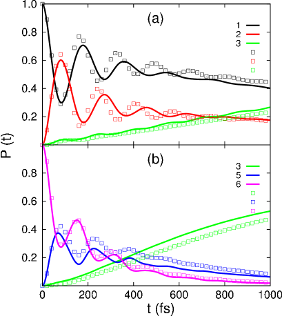
Figure 1: Population dynamics of selected FMO sites. In a), the population of sites $1$ (black), $2$ (red) and $3$ (green) with the initial condition $\rho(1,1)=1$ is shown, while in (b) the populations of sites $3$ (green), $5$ (blue) and $6$ (magenta) with the initial condition $\rho(6,6)=1$ is depicted (symbols: QUAPI, full lines: CMRT) for the parameters as given in the text.

IV.2 Two-dimensional spectra of a dimer system

To obtain 2D spectra, we combine the CMRT next with the PMA. This constitutes a very efficient approximate numerical tool whose reliability is assessed by a comparison with 2D spectra obtained by QUAPI. Since 2D spectra involve extended numerical calculations, QUAPI results are available only for small model systems with present day hardware technology. For such a comparison, we present the calculated results for the dimer model. It allows us to study energy transfer and dephasing (homogeneous broadening) as building blocks of the exciton dynamics in larger molecular compounds. It can still be treated by QUAPI with reasonable numerical effort.

Fig. 2 (left) shows 2D spectra of the dimer calculated by CMRT+PMA for $\lambda$=50 cm^-1 and the other parameters as indicated above. They are compared to QUAPI results (right column in Fig. 2) for waiting times $T=0$ fs, $50$ fs, $100$ fs and $500$ fs. These 2D spectra show two diagonal peaks (labeled A, B) which correspond to the two exciton states. Moreover, two cross peaks (labeled C and D) arise due to the excitonic coupling between them. For the sake of simplicity and clarity of the comparison, inhomogeneous broadening and the rotational averaging for different laser polarizations and molecular orientations is not performed here. Although this would be important to describe realistic experimental situations, the averaged results generally show smaller discrepancies (not shown).

At $T=0$ fs, the two results show the same profile for diagonal and cross peaks and, indeed, the agreement is excellent. This shows that the CMRT correctly models the coherence times and the system-bath correlations created during the simulation. With increasing waiting time, the same coherent dynamics is found for both the diagonal and the cross peaks and even can be inspected by eye. However, some disagreement is observed at long waiting time $T=500$ fs. The diagonal peak B in left figure (CMRT+PMA) shows a somewhat reduced amplitude as compared to the right figure (QUAPI).

For a more refined comparison, the amplitudes of the diagonal and cross peaks (A, B, C and D) are plotted against the waiting time in Fig. 3 and Fig. 4. In Fig. 3, the population dynamics of the diagonal peaks A (top) and B (bottom) calculated by CMRT+PMA from $0$ to $1000$ fs is shown and compared to the QUAPI result. We find that the CMRT+PMA provides reasonably accurate results for the population transfer and the oscillation period. However, the amplitude of peak B decays slightly faster in the approximate results as compared to the QUAPI data. Moreover, both yield different stationary states. In addition, the phase of the oscillations is slightly shifted. For the comparison of the cross peaks, the oscillatory behavior of peaks C and D is plotted in Fig. 4. Cross peak C shows a similar oscillatory behavior but the two approaches yield different stationary states. Peak D shows a only slightly shifted phase of the oscillatory behavior. Such a phase shift was also observed in the population dynamics of the FMO complex shown above. The phase shift might be due to the neglect of imaginary parts in the Redfield relaxation tensor.

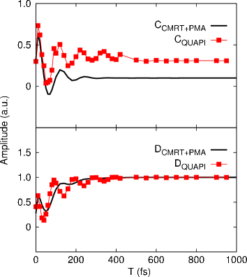
Figure 6: Oscillations of the cross peaks (C, D) with for a stronger system-bath interaction (same parameters as in Fig. 5). The cross-peak C calculated by CMRT+PMA yields a faster decay and a smaller amplitude (decay rates as obtained from a fit: CMRT+PMA: 62 fs, QUAPI: 177 fs).

In order to further assess the reliability of the CMRT+PMA, we have repeated the calculations for a larger reorganization energy, i.e., for $\lambda$=100 cm^-1 (with $\gamma$=100 cm^-1 kept unchanged). 2D spectra were again calculated by both approaches and the amplitude of the labeled peaks were extracted. Their time-dependence is plotted in Figs. 5 and 6. CMRT+PMA still yields quantitative agreement with the QUAPI result except for the behavior of the damping. The stronger system-bath coupling results in faster damping (diagonal peak A) and also in an increased difference between QUAPI and CMRT+PMA as compared to the weaker coupling with $\lambda$=50 cm^-1.

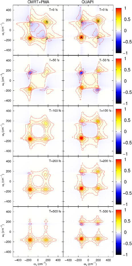
Figure 2: Two-dimensional photon-echo spectra of a dimer model calculated by CMRT+PMA (left) and QUAPI (right) for different waiting times as indicated. The Debye spectral density was used for the calculation with the parameters $\lambda=50$ cm^-1, $\gamma=100$ cm^-1 and the temperature was set to $T=77$ K.

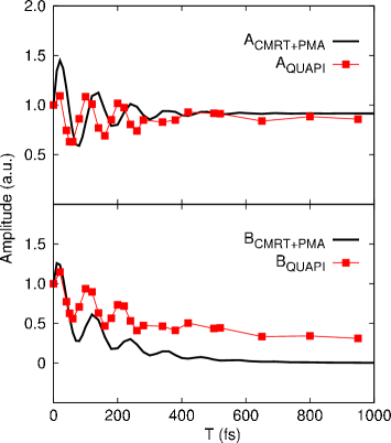
Figure 3: Population dynamics of the labeled diagonal peaks (A, B) extracted from the underlying sequence of 2D maps. The two approaches yield the same oscillation period. The diagonal peak B obatained from CMRT+PMA decays faster as compared to the QUAPI result. The oscillation periods can be extracted by data fitting and are: CMRT+PMA: 110fs, QUAPI: 99fs.

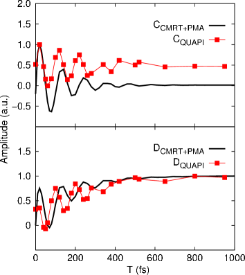
Figure 4: Coherent oscillations of labeled cross peaks (C, D) extracted from 2D maps. Cross peak C obained by CMRT+PMA shows the same oscillatory behavior, but with a somewhat smaller amplitude.

V Discussion – CMRT+PMA versus QUAPI

From the above comparison of the results obtained by both approaches, we observe that the discrepancies found in the 2D calculations are more pronounced than in the dynamics of the populations. Put differently, nonlinear 2D spectra are more sensitive to assess the performance and reliability of approximate theoretical approaches. In order to understand this, we point out two fundamental differences between 2D spectra and the population dynamics. First, entanglement between the system and the bath leads to initial correlations at the beginning of the waiting time window, which are absent in the calculation of the population dynamics. Second, two-exciton states contribute to the 2D spectra during the detection time, and interference between positive and negative peaks changes the observed amplitudes. This shows that one can not understand the reliability of a method to simulate correct 2D spectra by calculating population dynamics alone. Our current framework, in which we use the combined CMRT+PMA and compare the results with QUAPI, is well suited to show the performance of these methods in understanding 2D spectra directly.

In more detail, we have observed three noticeable discrepancies of the CMRT+PMA as compared to QUAPI: i) shifted oscillation phase of peak intensities, ii) a slightly faster decay, and, iii) a different amplitude of peaks B and C for long waiting times.

For the explanation of the shifted oscillation observed in 2D simulations of the CMRT+PMA, we need to notice that Eqs. 18, 19 provide the analytic result for a monomer (two-level system), and that this has been proven by comparing to QUAPI MRT_QUAPI . However, CMRT yields a shifted period for the dimer model. The mismatch is mainly caused by the population transfer term $R(t)$ since there is no population transfer term in the monomer model. In this paper, the population transfer rate was calculated by the cumulant expansion in Eq. 14 J Chem Phys 108 7763 (1998) and we only took the real part. It is well known that the imaginary part dominates the phase of the oscillations JCP 130 234111(2009) . So, most likely, the shifted oscillation is mainly caused by the real-value approximation of the population transfer rates.

Then, the population transfer term is also derived based on the second-order perturbation approximation, which is one of the reasons for the explanation of the slightly too fast decay of the oscillations found in CMRT calculations. Furthermore, the secular approximation was used to separate the population dynamics and the dephasing process in Eqs. 18, 19. This also contributes to the discrepancy in the decay rate, since it neglects the interference between population transfer and coherence dephasing.

A relatively small amplitude of peak B and C was found in Fig. 3 and Fig. 4 and it also can be observed by eye in the 2D map for the long waiting time $T=500$ fs. We observe that peaks B and C are mainly formed by one positive (red) peak and overlap with a negative (blue) peak in the 2D spectrum ($T=500$ fs). Therefore, the amplitude of those peaks mainly depends on the overlap of two peaks. In the QUAPI result, the two peaks are clearly separated with a larger spectral distance than in the CMRT result and this leads to the larger amplitude of peaks B and C in the 2D spectrum calculated with QUAPI. It indicates that, besides the shifted oscillation and the faster decay of the oscillation, CMRT does not properly account for the reorganization energy by the heat bath (diagonal peaks show slightly different positions in the 2D map: $-190$ cm^-1 and $190$ cm^-1 for CMRT and $-180$ cm^-1 and $200$ cm^-1 for QUAPI). In the CMRT, the reorganization energy is included in the diagonal part of the Hamiltonian by Eq. 3, where it just brings in a shift of the excitonic transition frequency $E_{\mu}$ by the renormalization term Eq. 3 and does not affect the dynamics of the off-diagonal terms in the Hamiltonian in Eq. (8).

Figure 5: Amplitude of the diagonal peaks A and B for a stronger system-bath coupling $\lambda$=100 cm^-1 (with $\gamma$=100 cm^-1 unchanged). CMRT+PMA calculations yield a faster decay (A) as compared to the QUAPI result (decay rate extracted from a fit: CMRT+PMA: 81 fs, QUAPI: 146 fs).

On the basis of a clear physical meaning (population transfer and dephasing terms) and for the purpose of an efficient and fast calculation, the secular approximation and the second-order perturbation theory were applied to construct the CMRT. On the one hand, the secular approximation leads to a separation of the population dynamics and dephasing process and avoids any complicated interaction terms between diagonal and off-diagonal parts in the equation of motion. On the other hand, the second-order perturbation theory simplifies the population transfers. It is possible to improve the equation by including higher orders. However, this renders the equation considerably more complicated and requires more computational resources for the simulation and it is a priori unclear how much this improves the accuracy.

VI Conclusions

In this paper we present the CMRT and compare it in more detail to the QUAPI method by calculating the population dynamics of selected FMO exciton sites and the 2D-spectrum of a model dimer. We found that CMRT provides numerical reliable results as compared to numerically exact QUAPI calculations for both the population dynamics and 2D spectra, as long as the reorganization energy is not too large compared to the typical energy gap of the system. Most importantly, it requires smaller computational efforts and orders of magnitude shorter calculation times. It provides us with an efficient approach to study the energy transfer in super-large molecular complexes and to perform complicated 2D simulations.

We found that the 2D profile calculated from CMRT+PMA agrees well with the corresponding QUAPI results. For a quantitative comparison, the amplitudes of diagonal and cross peaks were extracted from 2D maps and compared to those calculated by QUAPI. Quantitative agreement was found. We observe some discrepancies. In particular, oscillations are shifted, they decay slightly faster, and positions of peaks are slightly shifted. This becomes more serious if the reorganization energy is increased, which is also the case in Ref. MaMoix2 ; MaMoix1 .

The simulation protocol developed here can be used for arbitrary forms of the spectral density. One can envision an approach where the CMRT method is used to simulate super-large complexes, while numerically exact methods such as QUAPI play a role in benchmarking the accuracy of the simulations of smaller systems.

- (1) R. E. Blankenship, Molecular mechanisms of photosynthesis; Blackwell Science: Oxford; Malden, MA, 2002.
- (2) V. I. Prokhorenko, A. Halpin, and R. J. D. Miller, Opt. Express 17, 9764 (2009).
- (3) G. S. Engel, T. R. Calhoun, E. L. Read, T.-K. Ahn, T. Mančal, Y.-C. Cheng, R. E. Blankenship, and G. R. Fleming, Nature (London) 446, 782 (2007).
- (4) E. Collini, C. Y. Wong, K. E. Wilk, P. M. G. Curmi, P. Brumer, and G. D. Scholes, Nature 463, 644 (2010).
- (5) D. Zigmantas, E. L. Read, T. Mančal, T. Brixner, A. T. Gardiner, R. J. Cogdell, and G. R. Fleming, Proc. PNAS 103, 12672 (2006).
- (6) E. Romero, R. Augulis, V. I. Novoderezhkin, M. Ferretti, J. Thieme, D. Zigmantas and R. van Grondelle, Nature Phys. 10, 676 (2014).
- (7) F. D. Fuller, J. Pan, A. Gelzinis, V. Butkus, S. Seckin Sendlik, D. E. Wilcox, C. F. Yocum, L. Valkunas, D. Abramavicius, and J. P. Ogilvie, Nature Chem. 6, 706 (2014).
- (8) A. Ishizaki and G. R. Fleming, Proc. Natl. Acad. Sci. USA 106, 17255 (2009).
- (9) M. B. Plenio, J. Almeida, and S. F. Huelga, J. Chem. Phys. 139, 235102 (2013).
- (10) P. Nalbach, D. Braun and M. Thorwart, Phys. Rev. E 84, 041926 (2011).
- (11) M. Thorwart, J. Eckel, J. H. Rina, P. Nalbach and S. Weiss, Chem. Phys. Lett. 478, 234 (2009).
- (12) C. Kreisbeck, and T. Kramer, J. Phys. Chem. Lett. 3, 2828 (2012).
- (13) A. G. Redfield, Adv. Magn. Reson. 1, 1 (1965).
- (14) J. Adolphs, and T. Renger, Biophys. J. 91, 2778 (2006).
- (15) A. Ishizaki and G. R. Fleming, J. Chem. Phys. 130, 234110 (2009).
- (16) P. Nalbach and M. Thorwart, J. Chem. Phys. 132, 194111 (2010).
- (17) C. Mujica-Martinez, P. Nalbach and M. Thorwart, Phys. Rev. E 88, 062719 (2015).
- (18) W. M. Zhang, T. Meier, V. Chernyak and S. Mukamel, J. Chem. Phys. 108, 7763 (1998).
- (19) M. Yang, G. R. Fleming, Chem. Phys. 275, 355 (2002).
- (20) A. Gelzinis, L. Valkunas, F. D. Fuller, J. P. Ogilvie, S. Mukamel and D. Abramavicius, New J. Phys. 15, 075013 (2013).
- (21) V. I. Novoderezhkin, A. G. Yakovlev, R. van Grondelle, and V. A. Shuvalov, J. Phys. Chem. B 108, 7445 (2004).
- (22) Q. Ai, T. -C. Yen, B. -Y. Jin and Y. -C. Cheng, J. Phys. Chem. Lett. 4, 2577 (2013).
- (23) M. Cho et al. J. Phys. Chem. B 109, 10542 (2005).
- (24) K. L. M. Lewis, F. D. Fuller, J. A. Myers, C. F. Yocum, S. Mukamel, D. Abramavicius and J. P. Ogilvie, J. Phys. Chem. A 117, 34 (2013).
- (25) Y. Chang, and Y.-C. Cheng, J. Chem. Phys. 142, 034109 (2015).
- (26) M. Schröder, U. Kleinekathöfer and M. Schreiber, J. Chem. Phys. 124, 084903 (2006).
- (27) R. van Grondelle and V. I. Novoderezhkin, Phys. Chem. Chem. Phys. 8, 793 (2006).
- (28) Y.-H. Hwang-Fu, W. Chen, and Y.-C. Cheng, Chem. Phys. 447, 46 (2015).
- (29) S. Mukamel, Principles of nonlinear optical spectroscopy (Oxford University Press, New York, 1995).
- (30) O. Rancova, and D. Abramavicius, J. Phys. Chem. B 118, 7533 (2014).
- (31) G. S. Schlau-Cohen, T. R. Calhoun, N. S. Ginsberg, E. L. Read, M. Ballottari, R. Bassi, R. van Grondelle and G. R. Fleming, J. Phys. Chem. B 113, 15352 (2009).
- (32) D. Abramavicius, S. Mukamel, J. Chem. Phys. 134, 174504 (2011).
- (33) M. F. Gelin, D. Egorova and W. Domcke, J. Chem. Phys. 123, 164112 (2005).
- (34) L. Z. Sharp, D. Egorova, and W. Domcke, J. Chem. Phys. 132, 014501 (2010).
- (35) P. Nalbach, J. Eckel and M. Thorwart, New J. of Phys. 12, 065043 (2010).
- (36) J. Adolphs and T. Renger, Biophys. J. 91, 2778 (2006).
- (37) C. Meier and D. J. Tannor, J. Chem. Phys. 111, 3365 (1999).
- (38) M. Schröder, M. Schreiber, U. Kleinekathöfer, J. Luminescence, 125, 126 (2007).
- (39) V. May, O. Kühn, Charge and Energy Transfer Dynamics in Molecular Systems, (WILEY-VCH Press, Weinheim, 2011).
- (40) N. Makri and D. E. Makarov, J. Chem. Phys. 102, 4600 (1995).
- (41) N. Makri and D. E. Makarov, J. Chem. Phys. 102, 4611 (1995).
- (42) We compare the absorption lineshape calculated by CMRT and QUAPI. They show exactly same result.
- (43) A. Ishizaki, and G. R. Fleming, J. Chem. Phys. 130, 234111 (2009).
- (44) J. Ma, J. M. Moix, and J. S. Cao, J. Chem. Phys. 142, 094107 (2015).
- (45) J. M. Moix, J. Ma, and J. S. Cao, J. Chem. Phys. 142, 094108 (2015).