Detecting stellar spots through polarimetry observations of microlensing events in caustic-crossing

Abstract

In this work, we investigate if gravitational microlensing can magnify the polarization signal of a stellar spot and make it be observable. A stellar spot on a source star of microlensing makes polarization signal through two channels of Zeeman effect and breaking circular symmetry of the source surface brightness due to its temperature contrast. We first explore the characteristics of perturbations in polarimetric microlensing during caustic-crossing of a binary lensing as follows: (a) The cooler spots over the Galactic bulge sources have the smaller contributions in the total flux, although they have stronger magnetic fields. (b) The maximum deviation in the polarimetry curve due to the spot happens when the spot is located near the source edge and the source spot is first entering the caustic whereas the maximum photometric deviation occurs for the spots located at the source center. (c) There is a (partial) degeneracy for indicating spot’s size, its temperature contrast and its magnetic induction from the deviations in light or polarimetric curves. (d) If the time when the photometric deviation due to spot becomes zero (between positive and negative deviations) is inferred from microlensing light curves, we can indicate the magnification factor of the spot, characterizing the spot properties except its temperature contrast. The stellar spots alter the polarization degree as well as strongly change its orientation which gives some information about the spot position. Although, the photometry observations are more efficient in detecting stellar spots than the polarimetry ones, but polarimetry observations can specify the magnetic field of the source spots.

1 Introduction

Gravitational microlensing is an astronomical phenomenon in which the light of a background star is magnified due to passing through the gravitational field of a foreground object by producing distorted images Einstein (1936). This phenomenon has many applications in detecting extra-solar planets, measuring the mass of isolated stars, studying the stellar atmospheres, etc. (see, e.g. Mao 2012,Gaudi 2012).

One of features of gravitational microlensing is that it causes a net polarization for source stars Schneider & Wagoner (1987); Simmons et al. 1995a,b ; Bogdanov et al. (1996). There is a local polarization over the star surface due to the electron scattering in its atmosphere Chandrasekhar (1960). Since, these local polarizations have symmetric orientations with respect to the source center, the net polarization of a distant star is zero. Some effects can break this symmetry and create a net polarization for distant stars such as circum-stellar disk of dust grains around the central star Drissen et al. (1989); Akitaya et al. (2009), stellar spots, magnetic field and lensing effect. During a microlensing event, the circular symmetry of source star is broken and result is a net polarization for the source star. Measuring polarization during microlensing events helps us to evaluate the finite source effect, the Einstein radius and the limb-darkening parameters of source star Yoshida (2006); Agol (1996); Schneider & Wagoner (1987).

In single microlensing events, the polarimetric signal reaches to its maximum amount, i.e. about one percent, when the impact parameter of the source center i.e. $u_{cm}$ reaches to $\sim 0.96\rho_{\star}$ where $\rho_{\star}$ is the projected source radius, normalized to the Einstein radius Schneider & Wagoner (1987). But, the probability of happening a microlensing event with an impact parameter as smaller as $u_{cm}<\rho_{\star}$ is low. Whereas, in binary microlensing events whenever the source star crosses the caustic curve the polarization signal as high as one percent can be obtained Agol (1996). Indeed, the point-like caustic in a single lens converts to some closed curves in binary lensing which is extended about the angular Einstein radius (see e.g. Schneider and Weiss 1986).

Consequently, whenever the source crosses the caustic curves, due to the high gradient of magnification and polarization, the anomalies over the source surface can be resolved through photometric or polarimetric observations. One of the second-order perturbations over the source surface is the stellar spot. Indeed, a magnetic field over the source surface generates convective motions which make a temperature contrast with the source surface temperature, so-called as a stellar spot (e.g. Berdyugina 2005). A stellar spot produces a polarization signal through two channels (i) Zeeman effect due to its magnetic field and (ii) circular symmetry breaking of the source surface brightness due to the temperature contrast with the host star. Comparing these two effects, the first one has a dominant contribution in polarization signal. A stellar spot over the source surface disturbs the light and polarimetric curves of microlensing events. Detecting and characterizing stellar spots through their effects on the photometric light curves during microlenising events due to a point-like lens and binary lenses were extensively studied in (Heyrovský & Sasselov (2000),Han et al. (2000), Chang & Han (2002), Hendry et al. (2002), Hwang & Han (2010)). Here, we investigate detecting and characterizing stellar spots over the source surface through their effects on the polarimetric curves in microlensing events.

Although, most spot-induced polarization signals from the Galactic bulge sources are too weak to be detected by themselves, the lensing effect can magnify these signals and makes them be observable. Studying spot-induced perturbations in polarimetric microlensing due to a point-like lens was first investigated by Sajadian and Rahvar (2014). They also noticed that there is an orthogonal relation between the polarization orientation and the astrometric centroid shift vector in microlensing events due to a point-like lens and binary lenses except near the fold of caustic and investigated the advantages of this orthogonality for detecting the anomalies of the source surface. Here, we study detecting and characterizing the stellar spot through polarimetric microlensing in caustic-crossing. We first explore the characteristics of spot-induced perturbations on the polarization degree and its orientation in binary microlensing events. Then, by performing a Monte Carlo simulation from binary microlensing events with spotted sources during caustic-crossing we estimate the probability of detecting a stellar spot through polarimetric microlensing during caustic-crossing and the number of events.

In the following section, we study the stellar spot effects on (i) magnification factor, (ii) polarization degree and (iii) polarization orientations. In section (3) the detectability of the polarimetric and photometric deviations due to the stellar spots in microlensing events during caustic-crossing is studied by performing a Monte Carlo simulation. We explain the results in the last section.

2 spot-induced perturbation in polarimetric microlensing

In order to describe the polarized light we use the Stokes parameters of $S_{I}$, $S_{Q}$, $S_{U}$ and $S_{V}$. These parameters describe the total intensity, two components of linear polarization and circular polarization over the source surface, respectively Tinbergen (1996). The polarization degree $(P)$ and the polarization angles $\phi_{p}$ and $\theta_{p}$ as functions of Stokes parameters are given by Chandrasekhar (1960):

$$P = \frac{\sqrt{S_{Q}^{2}+S_{U}^{2}+S_{V}^{2}}}{S_{I}},$$

$$\phi_{p} = \frac{1}{2}\tan^{-1}{\frac{S_{U}}{S_{Q}}},$$

$$\theta_{p} = \frac{1}{2}\tan^{-1}{\frac{S_{V}}{\sqrt{S_{Q}^{2}+S_{U}^{2}}}}.$$ (1)

By considering the linear polarization of light scattering in a stellar atmosphere, the circular polarization is zero $S_{V}=0$. In microlensing events, the Stokes parameters during the magnification are given by:

$$\left(\begin{array}[]{c}S_{Q,\star}\\ S_{U,\star}\end{array}\right) = \rho^{2}_{\star}\int_{0}^{1}\rho~{}d\rho\int_{-\pi}^{\pi}d\phi I_{-}(\mu)A(u)\left(\begin{array}[]{c}-\cos 2\phi\\ \sin 2\phi\end{array}\right),$$ (6)

$$S_{I,\star} = ~{}\rho^{2}_{\star}\int_{0}^{1}\rho d\rho\int_{-\pi}^{\pi}d\phi I(\mu)~{}A(u),$$ (7)

where $\rho_{\star}$ is the projected source radius which is normalized to the Einstein radius, $\rho$ is the distance from the centre of the stellar disk to each element over the source surface which is normalized to the source radius, $\mu=\sqrt{1-\rho^{2}}$, $\phi$ is the azimuthal angle between the lens-source connection line and the line from the center of coordinate to each element over the source surface, $u=(u_{cm}^{2}+\rho^{2}\rho^{2}_{\star}+2\rho\rho_{\star}u_{cm}\cos\phi)^{1/2}$ is the distance of each projected element over the source surface with respect to the lens position, $u_{cm}$ is the impact parameter of the source center and magnification factor for simple microlensing is $A(u)=\frac{u^{2}+2}{u\sqrt{u^{2}+4}}$. The amounts of $I(\mu)$ and $I_{-}(\mu)$, as the total and polarized light intensities, by assuming the electron scattering in spherically isotropic scattering atmosphere of an early-type star on the emitted light, were evaluated by Chandrasekhar (1960) as follows:

$$I(\mu) = I_{\star}(1-c_{1}(1-\mu)),$$

$$I_{-}(\mu) = I_{\star}c_{2}(1-\mu),$$ (8)

where $I_{\star}$ is the source intensity at the disk center, $c_{1}=0.64$ and $c_{2}=0.032$ Schneider & Wagoner (1987). Here, we focus on the giant sources with finite size effect for which the limb-darkening coefficients are different a bit. For these sources, we set $c_{1}=0.7$ Zub et al. (2009) and $c_{2}=0.04$.

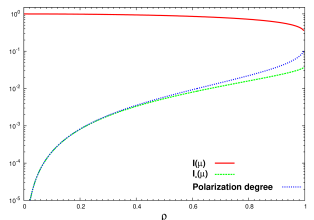
Figure 1: $I(\mu)$ the total intensity (solid red line), $I_{-}$ the polarized intensity (green dashed line) normalized to the source intensity at the disk center, i.e. $I_{\star}$, and the polarization degree (blue dotted line) versus the distance from the source center normalized to the source radius i.e. $\rho$.

Figure (1) represents $I(\mu)$ (red solid line), $I_{-}(\mu)$ (green dashed line), normalized to the intensity of the source at the disk center, versus the distance from the source center normalized to the source radius i.e. $\rho$. According to this figure, considering the limb-darkening effect the total intensity $I(\mu)$ decreases a bit whereas the polarized intensity $I_{-}(\mu)$ increases from the center to the limb. If there is no lensing effect i.e. $A(u)=1$, the local polarization degree is equal to $P=I_{-}(\mu)/I(\mu)$. Here, over the star surface the polarization degrees enhance from the center to limb as shown in Figure (1) with blue dotted line. Also, the polarization vector in each point of the source surface is tangent to a circle whose center coincides to the source center and passes from that point. The overall polarization signal of an ideal source is zero, because of the symmetric orientations of local polarizations with respect to the source center.

Now, let us consider a stellar spot on the source surface. To specify the spot in our simulation, we use four parameters for spots as: (i) the size of spot, (ii) the location of spot on the source star, (iii) its magnetic field and (iv) the temperature contrast of the spot with respect to the host star. These parameters are not completely independent and there is a correlation relation between the magnetic field of the spot and its temperature contrast with respect to the host star Berdyugina (2005). Also, we consider the following limitations for modeling the spot polarization: (i) There is one circular spot on the source surface, (ii) the magnetic field over the spot has a constant amount and its direction is radial, (iii) the magnetic field is high enough to ignore the Hanle effect (see e.g. Stenflo (2013)), (iii) we take the Minle-Eddington model for the stellar atmosphere in which the line source function is linear versus the optical depth, (iv) the ratio of the line and continuous absorption coefficients is constant, (v) the intensity over the spot is constant. Also we assume a black body radiation for the spot and its host star to indicate their intensities and finally (vi) we estimate the broad band Stokes intensities by integrating over the wavelength pass band, taking into account the Stokes intensities in a spectral line.

The radius of the spot is $r_{s}$ and the angular radius of spot in coordinate located at the centre of source star is given by $\theta_{0}=\sin^{-1}(r_{s}/R_{\star})$. We preform a coordinate transformation to obtain the position of spot on the lens coordinate set two axes of which describe the sky plane. In this regard, we use the two rotation angles of $\theta_{s}$ around $y$-axis and $\phi_{s}$ around $z$-axis. The more details about modeling of the spot in our simulation can be found in Sajadian and Rahvar (2014).

To calculate the modified Stokes parameters, we integrate over the source surface from the Stokes intensities. Since, the Stokes intensities over a given spot are different from those over the other points of the source surface, we take into account the combination of the terms from spot and source star, using a step function. The overall Stokes parameters $S^{\prime}_{Q}$, $S^{\prime}_{U}$, $S^{\prime}_{V}$ and $S^{\prime}_{I}$ are given by:

$$\left(\begin{array}[]{c}S^{\prime}_{Q}\\ S^{\prime}_{U}\\ S^{\prime}_{V}\\ S^{\prime}_{I}\end{array}\right)=\rho_{\star}^{2}~{}\int_{0}^{1}\rho d\rho~{}\int_{-\pi}^{\pi}d\phi A(u)\{~{}~{}~{}~{}~{}~{}~{}~{}~{}~{}~{}~{}~{}~{}~{}~{}~{}~{}~{}~{}~{}~{}~{}~{}~{}~{}~{}~{}~{}~{}~{}~{}~{}~{}~{}~{}~{}~{}~{}~{}~{}~{}~{}$$ (13)

$$(1-\Theta(\rho,\phi))\left(\begin{array}[]{c}-I_{-}(\mu)\cos 2\phi\\ I_{-}(\mu)\sin 2\phi\\ 0\\ I(\mu)\end{array}\right)+\Theta(\rho,\phi)~{}\left(\begin{array}[]{c}I_{Q,s}\\ I_{U,s}\\ I_{V,s}\\ I_{I,s}\end{array}\right)~{}\},$$ (22)

where $\Theta(\rho,\phi)$ is that step function which is equal to one within the spot area and zero for the other points. $I_{Q,s}$, $I_{U,s}$, $I_{V,s}$ and $I_{I,s}$ are the Stokes intensities over the spot which are measured according to the spot position, it magnetic field and its intensity. Indeed, the magnetic field through the Zeeman effect on the spectral lines causes a net polarization for the spot which is mostly circular (see e.g. Illing et al. 1975). The more details about calculating these Stokes intensities by considering the mentioned limitations over the source and its atmosphere are brought in Appendix section.

The spot-induced perturbations on the magnification factor, polarization degree and polarization angles are explained in the following subsections respectively.

2.1 Perturbation on the magnification factor

The spot-induced perturbation on microlensing light curve due to a point-like lens was first investigated by Heyrovský and Sasselov (2000). They concluded that the photometric spot effect can numerically reach the fractional spot radius. Then, the feasibility of spot detection, studying the spot-induced perturbations in binary microlensing events during the caustic crossing and delectability of spot in different wavelengths have been discussed in details by a number of authors Han et al. (2000); Chang & Han (2002); Hwang & Han (2010); Hendry et al. (2002).

To calculate the magnification factor of a spotted source, we assume that the intensity of the spot, i.e. $I_{I,s}$, is almost constant over the spot area. Hence, we can re-write the fourth modified Stokes parameter $S^{\prime}_{I}$ (in equation 13), by factoring out $I_{I,s}$ as:

$$S^{\prime}_{I} \cong S_{I,\star}-b~{}I(\mu_{s})~{}\rho_{\star}^{2}\int_{0}^{1}~{}\rho~{}d\rho~{}\int_{-\pi}^{\pi}d\phi~{}A(u)~{}\Theta(\rho,\phi)$$ (23)

$$= S_{I,\star}-b~{}S_{I,s},$$

where we define $b~{}\equiv~{}(I(\mu_{s})-I_{I,s})/I(\mu_{s})$, $I(\mu_{s})$ is the source intensity at the geometrical location of the spot center i.e. $(\theta_{s},\phi_{s})$, $\mu_{s}=\cos\theta_{s}$, $S_{I,\star}$ is the Stokes parameter due to the source without any spot, given by equation (6) and $S_{I,s}$ is the Stokes parameter of the spot itself considering $I(\mu_{s})$ as its intensity. Integrating is done over the source area. In that case, the magnification factor of a spotted source is given by:

$$A^{\prime}=\frac{S_{I,\star}-b~{}S_{I,s}}{S_{I,\star,0}-b~{}S_{I,s,0}}=A\frac{1-b\beta}{1-b\delta},$$ (24)

where the index $0$ of the Stokes parameters refers to the ones without lensing effect. $A=S_{I,\star}/S_{I,\star,0}$ is the magnification factor of the source without any spot, $\beta=S_{I,s}/S_{I,\star}$ and $\delta=S_{I,s,0}/S_{I,\star,0}$. The magnification factor $A^{\prime}$ up to the third order in $\delta$ in terms of un-perturbed magnification factor $A$ and perturbation terms is given by:

$$A^{\prime}=A[1+b(\delta-\beta)+b^{2}\delta(\delta-\beta)+b^{3}\delta^{2}(\delta-\beta)+....].$$ (25)

Here, a spot on the surface of source star has two effects: (i) decreasing the baseline flux of the source which enhances the magnification factor by $b\delta+b^{2}\delta^{2}+...$ and (ii) decreasing the magnified light which decreases the magnification factor about $-b\beta-b^{2}\beta\delta-...$. Before the spot reaches to the caustic curve, the magnification factor enhances due to the first effect. When the spot light is being magnified due to passing over the caustic line or approaching to the lens position, the second effect dominates and the total magnification factor decreases. When these two effects have the same amounts i.e. $\beta=\delta$, the perturbation terms vanish. In this time, $A^{\prime}=A=A_{s}$ where $A_{s}=\frac{S_{I,s}}{S_{I,s,0}}$ which means that the magnification factor of the source is equal to the magnification factor of the spot itself. This time does not depend on the relative difference in the intensity of source and spot i.e. $b$ and just depends on the spot area and its location with respect to the lens or caustic line. If the source radius and the lens position (or the caustic configuration in binary lensing) in this time are deduced from the photometric observations, we can assign the magnification factor of the spot itself which helps us to characterize the spot properties.

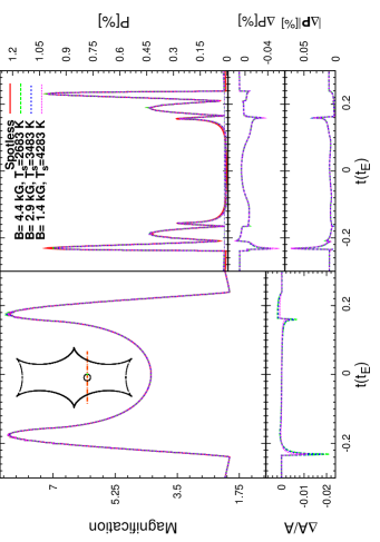
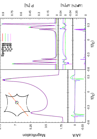
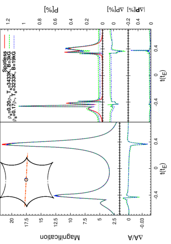
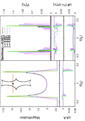
Figure 2: Example microlensing events affected with source spot. In every subfigure, the light curves and polarimetric curves are shown in left and right panels. The source (black circle) and its spot located over the source surface, caustic curve (black curve) and source centre trajectory projected in the lens plane (red dash-dotted line) are shown with insets in the left-hand panels. The thinner lines in right panel show the spot polarization signal without lensing effect. The simple models without spot effect are shown by red solid lines. The photometric and polarimetric residuals with respect to the simple models are plotted in bottom panels. Note that the top polarimetric residuals are the residual in the polarization degree $\Delta P$ and the bottom ones are the absolute value of the residual in the polarization vector $|\boldsymbol{\Delta P}|$. The parameters used to make these microlensing events can be found in Table (1).

2.2 Perturbation on the polarization degree

Here, we investigate the spot-induced perturbations on polarization degree during a microlensing event, some prospects are explained in the following.

(a) Berdyugina (2005) noticed that there are some correlation relations between the spot parameters such as its magnetic field, temperature contrast and the source photosphere temperature. She plotted the data of magnetic field measurement $B(kG)$ and the spot temperature contrast $\Delta T(K)$ versus the photosphere temperature $T_{\star}(K)$ for some active dwarfs and giants and concluded that the hotter giants have the weaker magnetic field whereas their spots have the higher temperature contrast. We can fit two useful functions to her data which are given by:

$$\Delta T(K) = 1.26\times 10^{-4}T_{\star}^{2}-0.53T_{\star}+787.40,$$

$$B(kG) = -1.06\times 10^{-3}~{}T_{\star}+7.46.$$ (26)

According to these relations, for a source star with a constant photosphere temperature, the cooler stellar spots have the stronger magnetic fields and as a result the higher polarization signals.

On the other hand, the Stokes intensities of the spot, i.e. $I_{i,s}$ (for $i=Q,U,V,I$), are proportional to the continuum, local intensity of the spot, i.e. $I_{c}$, (for more details see Appendix section). But, in the microlensing observations from the sources in the Galactic bulge, we receive the total flux of the source and its spot. Hence, the darker spots have the smaller contributions to the total flux whereas they intrinsically have larger polarization signals due to the stronger magnetic fields. Here, we investigate which of these two effects, i.e. (1) the spot magnetic field and (2) the spot flux contrast, has more contribution in the polarimetric perturbations in microlensing events.

	Figure number	$M_{\star}(M_{\odot})$	$R_{\star}(R_{\odot})$	$T_{\star}(K)$	$\rho_{\star}$	$r_{s}(R_{\star})$	$T_{s}(K)$	$B(kG)$	$\theta_{s}^{\circ}$	$\phi_{s}^{\circ}$	$u_{cm}$	$\xi^{\circ}$	$d$	$q$
	$2(a)$	$2.6$	$24.9$	$4314$	$0.04$	$0.35$	$--$	$--$	$70$	$0$	$-0.15$	$0$	$1$	$1$
	$2(b)$	$2.8$	$28.4$	$4302$	$0.05$	$0.35$	$3477$	$2.9$	$--$	$40$	$0.01$	$40$	$1.2$	$0.5$
	$2(c)$	$1.9$	$17.2$	$4206$	$0.03$	$0.30$	$--$	$--$	$55$	$23$	$0.01$	$-3$	$1.2$	$0.8$
	$2(d)$	$1.2$	$4.5$	$4492$	$--$	$0.3$	$3495$	$2.7$	$-45$	$10$	$0.15$	$0$	$0.9$	$0.9$
	$(3)$	$2.8$	$28.4$	$4302$	$0.05$	$0.35$	$3477$	$2.9$	$40$	$0$	$0.01$	$40$	$1.2$	$0.5$

Table 1: The table contains the parameters used to make the microlensing events shown in Figures 2, 2, 2, 2 and (3) respectively. These parameters are the source mass $M_{\star}(M_{\odot})$, the source radius $R_{\star}(R_{\odot})$, the photosphere temperature of the source $T_{\star}(K)$, the projected source radius in the lens plane, normalized to the Einstein radius $\rho_{\star}$, the spot radius normalized to the source radius $r_{s}(R_{\star})$, the spot temperature $T_{s}(K)$, the spot magnetic field $B(kG)$, the spot projection angles $\theta_{s}^{\circ}$ and $\phi_{s}^{\circ}$, the impact parameter of the source center $u_{cm}$, the angle between the trajectory of source star and the binary axis $\xi^{\circ}$, the distance between two lens normalized to the Einstein radius $d$ and the mass ratio of two lens $q$ respectively. The giant stars as sources are chosen from a synthetic distribution for giant stars made from Besançon model (Robin et al. 2003). For these figures, we also set the mass of the primary lens $M_{l}=0.3~{}M_{\odot}$, the lens and source distance from the observer $D_{l}=6.5~{}kpc$ and $D_{s}=8.0~{}kpc$ and the limb-darkening coefficients $c_{1}=0.7$ and $c_{2}=0.04$.

For this aim, in Figure 2 we show a polarimetric microlensing event affected by the source spot. We consider a giant star as the source with the parameters $T_{\star}(K)=4314$, $M_{\star}(M_{\odot})=2.6$ and $R_{\star}(R_{\odot})=24.9$. Also we assume that the source has a spot with the parameters $\Delta T(K)=831$ and $B(kG)=2.9$, chosen according to the equations (2.2). In addition, we consider a cooler spot with a stronger magnetic field and the hotter spot with a weaker magnetic field. The light curves and polarimetric curves for these three cases are shown in left and right panels of this figure. The source (black circle) and its spot located over the source surface, caustic curve (black curve) and source center trajectory projected in the lens plane (red dash-dotted line) are shown with an inset in the left-hand panel. The thinner lines in right panel show the intrinsic polarization signals of the spotted source. The simple models without spot effect are shown by red solid lines. The photometric and polarimetric residuals with respect to the simple models are plotted in bottom panels. Note that the polarimetric residuals are the residual in the polarization degree without considering the polarization angles i.e. $\Delta P$ and the absolute value of the residual in the polarization vector i.e. $|\boldsymbol{\Delta P}|$ whose definition is brought in equation (27). The parameters used to make this microlensing event can be found in Table (1). To calculate the magnification factor of each element over the source star, we use the adaptive contouring algorithm Dominik (2007). According to this figure three spots with different magnetic fields and temperature contrasts have almost the same intrinsic polarization signals and as a result the same polarimetric deviations in the polarimetric microlensing. Hence, these two effects whereas act reversely have the same strengths. The photometric signature of the spot depends on the temperature contrast and enhances with increasing it.

The polarization signal of spot maximizes when the spot is crossing the caustic curve. If the spot is located on the source edge and the source is entering into the caustic from that edge (near the spot), the spot-induced perturbation is so higher than when that source is coming out from that edge. Because, in the first case the light from the other points over the source surface is not magnified. Accordingly, in the first caustic-crossing of Figure 2, the spot-induced perturbation is higher than that in the second one.

Also, the duration of the polarimetric signal depends on the location of spot with respect to the caustic line, the size of spot and its host star and it does not depend on the temperature contrast and the magnetic field.

(b) The effect of the projection angle $\theta_{s}$ on the spot-induced polarimetric deviation: the amount of the circular Stokes intensity in a spectral line due to Zeeman effect is proportional to $\cos\theta_{s}$ and as a result increases by decreasing $\theta_{s}$, whereas the linear Stokes intensities in a spectral line are proportional to $\sin^{2}\theta_{s}$ and decrease by decreasing $\theta_{s}$ (see equations A and A in Appendix section). Hence, the polarization signals due to face-on spots are more circular and those due to spots with larger projection angles are more linear. As mentioned in the Appendix section, the broadband circular Stokes intensity is so smaller than that in a spectral line by one order of magnitude whereas the linear ones have almost the same amounts as those in a spectral line. Because, the circular polarization in a spectral line has an anti-symmetric shape with respect to the wavelength. Consequently, stellar spots with the smaller projection angle $\theta_{s}$ have lower polarized Stokes intensities.

In Figure 2 a polarimetric microlensing event of a spotted source is represented with three different amounts of the projection angle $\theta_{s}$. According to this figure, the intrinsic polarization signal due to the spot without lensing for $\theta_{s}=10^{\circ}$ (about $0.005$ per cent) is so smaller than that with $\theta_{s}=45^{\circ}$ (about $0.026$ per cent), shown with thin, straight lines. On the other hand, increasing the projection angle $\theta_{s}$ decreases the spot area and the total intensity considering limb-darkening effect and as a result increases $S^{\prime}_{I}$ (which decreases the polarization signal). Therefore, by increasing the projection angle, the polarization signal due to stellar spots without lensing increases and then decreases. The polarization signal without lensing due to the spot with $\theta_{s}=80^{\circ}$ is equal to $0.018$ per cent, lower than that with $\theta_{s}=45^{\circ}$.

However, the deviations in the polarimetric microlensing due to the spot with $\theta_{s}=80^{\circ}$ is a bit larger than that due to the spot with $\theta_{s}=45^{\circ}$ which is due to the finite size effect. The larger projection angle, the smaller area of the spot. In microlensing events, finite size effect always shrinks sharp signals.

In the photometric curves, increasing the projection angle $\theta_{s}$ decreases the spot-induced photometric signal. Because, the spot area decreases by increasing the projection angle by $\cos\theta_{s}$ which decreases the spot-induced perturbation signal. However, the total intensity decreases from the center to the limb of the source star due to limb-darkening effect (see Figure 1), but this effect is so smaller than the first one. If the area of the spot is fixed by considering the limb-darkening effect, the photometric signal due to the spot does not change significantly (see e.g. Heyrovský & Sasselov (2000)). Therefore, the spots located at the source center make higher photometric signals as shown in Figure 2. This points was also noticed by Hendry et al. (2002).

(c) There is a partial degeneracy for indicating the spot size and its temperature difference with respect to the host star from the photometric deviations. However, these two factors are not completely degenerate. Because by increasing the spot size the finite size effect becomes important. This effect strongly alters the shape of the spot-induced signals. Whereas, increasing the spot temperature contrast only increases the perturbation signals and does not change the shape of the signals. Hence, these two effect are partially degenerate in the photometric measurements. Although, two degenerate spots with the same photometric deviations have different, intrinsic polarization signals, but by considering two different magnetic fields, they can have the same polarization signal and be polarimetrically degenerate. In Figure 2, we make two microlensing events with spotted sources in which the spots have the same positions but different sizes, temperature differences and magnetic fields. These spots have the same, intrinsic polarization signals. These two events have the same light and polarimetric curves and are degenerate. However, in the photometric curve degeneracy is between the spot size and its temperature contrast. Therefore, we can not uniquely extract the spot properties from the photometric or polarimetric deviations.

(d) We investigate the finite size effect on the photometric and polarimetric signals due to the spot. The spot-induced perturbations decrease and lengthen with increasing the source radius. Because, by integrating over the source surface, the sharp signals due to the points located at the caustic line shrink. In Figure 2, we represent a microlensing event with three different amounts of $\rho_{\star}$ and considering $r_{s}=0.3~{}R_{\star}$. The residual for each source size is calculated from the spotless source of that particular size.

2.3 Perturbation on the angle of polarization

The polarization angle $\phi_{p}$ strongly changes due to the stellar spot. Because, this polarization angle is not related to the total Stokes parameter, i.e. $S^{\prime}_{I}$ which is very larger than the polarized Stokes parameters. On the other hand, the polarization angle $\theta_{p}$ alters a bit. Because, the broad band circular polarization of spots is, one order of magnitude, smaller than the linear ones. The spot-induced perturbation in the polarization angle causes the polarization vector alters as follows:

$$|\boldsymbol{\Delta P}|=[P^{\prime 2}+P^{2}-2P^{\prime}P\cos\theta_{p}^{\prime}\cos(\phi_{p}^{\prime}-\phi_{p})]^{1/2}.$$ (27)

Indeed, we define the polarization vector as $\boldsymbol{P}=(P\cos\theta_{p}\cos\phi_{p},P\cos\theta_{p}\sin\phi_{p},P\sin\theta_{p})$. Note that in normal microlensing events without spot effect $\theta_{p}=0$. In Figure (3) we show the curves of the polarization angle $\phi_{p}$ (left panel) and polarization degree (right panel) of a microlensing event.

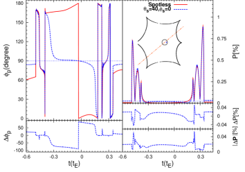
Figure 3: A polarimetric microlensing event due a spotted source: The curves of polarization angle $\phi_{p}$ and the polarization degree are shown in the left and right panels. The simple models without spot effect are shown by red solid lines. The polarimetric residuals with respect to the simple models are plotted in the bottom of each panel. The parameters used to make this microlensing event can be found in Table (1).

Measuring the polarization angles helps us to indicate the different components of the polarized intensity which gives some information about the projection angles $\theta_{s}$ and $\phi_{s}$. On the other hand, measuring the polarization angles in addition to the polarization degree can increase detectability of stellar spots through polarimetric measurements, e.g. in Figure 2 although the maximum amount of the residual in the polarization degree $\Delta P$ due to the spot reaches to $0.04$ per cent, but by considering the variation of the polarization angles, the residual in the polarization vector rises up to $0.35$ per cent.

3 Observational prospects

In the previous section we studied the spot-induced perturbations during caustic-crossing in binary microlensing events. Now, we estimate the probability of detecting the source spots in polarimetric or photometric observations during caustic crossing. In this regard, we perform a Monte Carlo simulation by generating many synthetics caustic-crossing microlensing events with spotted and giant sources. By considering two useful criteria for polarimetric and photometric observations, we survey if the spot-induced perturbations can be discerned in each light curve or polarimetric curve. Finally, we estimate the number of events with detectable spot-induced signals for given amounts of background stars and observational time.

Our criterion for detectability of source spots in the microlensing light curves is $(A^{\prime}-A)/A\geq 2$ per cent. For polarimetric measurements, we assume that these observations are done by the FOcal Reducer and low dispersion Spectrograph (FORS2) polarimeter at Very Large Telescope (VLT) telescope. This polarimeter can achieve to the polarimetric precision about $0.1$ per cent with one hour exposure time from a source star brighter than $14.5$ mag Ingrosso et al. (2015). To evaluate the detectability of the polarimetric signals due to the source spots, for each microlensing event we evaluate signal to noise ratio (SNR) when the spot is crossing the caustic curve, which is given by:

$$SNR=\sqrt{[10^{-0.4m_{\star}}A^{\prime}+\Omega_{PSF}10^{-0.4\mu_{sky}}]t_{exp}10^{0.4m_{zp}}},$$ (28)

where, $m_{\star}(mag)$ is the apparent magnitude of the source star, $A^{\prime}$ is the magnification factor of the spotted source, $\Omega_{PSF}$ is the area of the Point Spread Function (PSF), $\mu_{sky}=22.5(mag/arcs^{2})$ is the sky brightness, $t_{exp}(s)$ is the exposure time and $m_{zp}=28.3(mag)$ is the zero point magnitude of FORS2 polarimeter at VLT. We assume that there is no blending effect. For detecting the spot signal, the exposure time should be less than the time when the spot is crossing the caustic curve and we set $t_{exp}=t_{E}\rho_{s}/3$ where $\rho_{s}$ is the spot radius projected in the lens plane and normalized to the Einstein radius. The threshold amount of SNR to achieve the polarimetric precision about $0.1$ per cent is about $SNR_{thr}=34000$. Hence, our criteria for detectability of the source spot in the polarimetric curves are $|\boldsymbol{\Delta P}|>0.1$ per cent as well as $SNR>SNR_{thr}$.

Here, the distribution functions of the binary lenses, source and its spot parameters used to generate syntectic binary microlensing events are illustrated. We explained the distribution functions for the mass of the lenses, the Galactic coordinates and velocities of both sources and lenses, the mass ratio for the binary lenses and their distance as well as the source trajectory with respect to the binary axis in our previous works Sajadian (2014, 2015), and do not repeat them here.

We consider only giant stars as sources. For indicating the mass, surface temperature, absolute magnitude and radius of giant sources, we make an ensemble of giant stars using Besançon model Robin et al. (2003). Then, we choose the source stars from that ensemble randomly. We obtain the apparent magnitude of the source star $(m_{\star})$ according to the absolute magnitude, distance modulus and extinction. In that case, the more details can be found in Sajadian (2015). Also, I consider constant amounts for limb-darkening coefficients of source stars as $c_{1}=0.7$ and $c_{2}=0.04$.

For the spot, we indicate its magnetic field and temperature contrast using the equation (2.2) and adding Gaussian fluctuations. There is a correlation relation between the magnetic field of spots and the filling factor, i.e. the total fractional area covered by the spot, as $f=0.4~{}B(kG)-0.7$ Berdyugina (2005). In the simulation we consider only one spot over the source surface. For the Galactic bulge stars, only the biggest spot can probably be detected. We need the distribution function of the radius of the biggest spots over source stars. I assume that the ratio of the area of the biggest spot to the total area due to all spots over the Sun is the same as that ratio due to the spots over other stars. This ratio for the Sun spots is about $0.04$ Solanki (2003). Therefore, I first indicate the total fractional area due to the spots, i.e. $f$, according to the magnetic field by adding a Gaussian fluctuation and then multiply it by $0.04$ to indicate the fractional area due to the biggest spot.

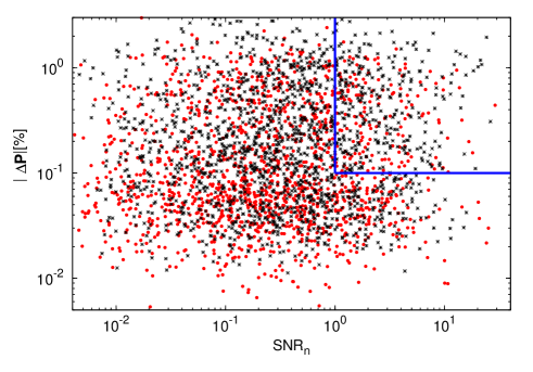
Figure 4: The scatter plot of the spot-induced polarimetric signals in synthetic microlensing events versus SNR which is normalized to the threshold amount. The blue solid line separates the microlensing events with detectable polarimetric signatures due to the spot. The black stars represent the microlensing events with detectable photometric signals due to the spot and red circles show the events in which the spot-induced signatures can not be discerned through photometric observations.

In order to obtain the spot position in the lens plane, we need two rotation angles of $\theta_{s}$ around $y$-axis and $\phi_{s}$ around $z$-axis. $\phi_{s}$ is uniformly taken in the range of $[0,\pi]$. We choose $\theta_{s}$ by fixing the angular surface element. Hence, we uniformly select $\psi$ in the range of $[-1,1]$ where $\theta_{s}=cos^{-1}\psi$. For the broadband Stokes intensities due to the magnetic field, we first calculate them in a spectral line and then by considering the factor $a$ (introduced in the Appendix section) estimate the amounts of these Stokes intensities. Finally, we investigate with how many probability lensing magnifies these polarization signals and makes them be observed.

Having performing the Monte Carlo simulation, we concluded that in about $11.2$ per cent of the simulated events the spot-induced polarimetric signals are detectable according to our criteria. Note that the real efficiency is certainly less than this number. Indeed, in observations of microlensing events, 3-5 consecutive data points with deviations more than 2-3$\sigma$ with respect to the simple model are needed to confirm a perturbation effect, where $\sigma$ is the observational accuracy (see e.g. Dominik et al. 2010). But in this Monte Carlo simulation, we do not simulate the data points. Hence, short-duration spot-induced signals (e.g. see Figure 2) which are detectable according to our criteria would be difficult to detect in real observations due to data spacing and may be confused with the noise. On the other hand, observers should fit many synthetic light and polarimetric curves with different perturbations to the data points. Therefore during observation the true event can be confused with other microlensing events which are well fitted to the data points e.g. the perturbation due to the stellar spots can be mistaken with a transit exo-planet around the source star.

In Figure (4), we represent the scatter plot of the spot-induced polarimetric signals, i.e. $|\boldsymbol{\Delta P}|$ for synthetic microlensing events versus SNR normalized to the threshold amount i.e. $SNR_{n}$. The blue solid line separates the microlensing events with detectable polarimetric signatures due to the spot from the others.

According to the OGLE-III data Wyrzykowski et al. (2014), about $f_{1}=18.4$ per cent of the microlensing sources are giant stars and about $f_{2}=5.4$ per cent of microlensing events are due to the binary lenses with caustic-crossing features. Generally, all giant stars are not magnetically active. RS CVn-type binaries, FK Comae-type giants and Lithium rich giants have high magnetic activity Korhonen (2013). Recently for some of other giant stars magnetic fields have been detected and even mapped (e.g. Strassmeier et al. 1990, Aurière et al. 2008, Dorch 2004). Indeed, the magnetic activity decreases with the age Skumanich (1972). Consequently, I assume that about $f_{3}=1$ per cent of giant stars have stellar spots and magnetic field stronger than $100$ G. The probability of detecting a spot over a giant source through polarimetric measurements in caustic-crossing of microlensing events can be given by:

$$\tau_{s}=\epsilon~{}f_{1}~{}f_{2}~{}f_{3}~{}\tau,$$ (29)

where $\epsilon=0.112$ is the polarimetric efficiency for detecting spot-induced signals in the simulated events, $\tau$ is the optical depth for the microlensing events towards a given direction. For the direction of the Galactic Bulge $\tau=4.48\times 10^{-6}$ Sumi et al. (2006), hence the optical depth for the polarimetric spot detection is $\tau_{s}=4.99\times 10^{-11}$. Finally, we estimate the number of events for $N_{bg}$ background stars being detected during the observational time $T_{obs}$ as

$$N_{s}=\frac{\pi}{2}\frac{T_{obs}N_{bg}}{<t_{E}>}\times\tau_{s},$$ (30)

where the average Einstein crossing time for the Galactic Bulge events due to the giant sources is about $<t_{E}>=24.6$  days Wyrzykowski et al. (2014). By monitoring $150$ million objects during $10$ years towards the Galactic bugle, the number of binary microlensing events with spotted and giant sources, which have detectable spot-induced polarimetric signals, is $1.75$. Finally, we investigate in how fraction of these simulated events the photometric spot-induced signal $(A^{\prime}-A)/A$ is greater than $2$ per cent. In this regard, the photometric efficiency for detecting signatures due to the spot is $52.6$ per cent. In that case the number of events during $10$ years observations from $150$ million objects will be $8.19$. Note that, we consider only giant stars as sources and do not consider main-sequence stars. In Figure (4) the black stars show these events which have detectable photometric signatures due to the spot.

Consequently, photometry observation is more efficient in detecting stellar spots than the polarimetry observation. However, polarimetry observations during microlensing events give us some information about the magnetic field of the spots over the sources whereas the photometric signals due to the spots do not depend on it. On the other hand, the stellar spots change polarization orientation in addition to the polarization degree whereas in the photometric observations of spotted sources only the magnification factor alters. Variation of the polarization angles give us extra information about the different components of the polarized intensity and as a result the position of spot on the source surface. Also, the polarimetry observations can be complementary to the photometry observations for detecting stellar spots with larger amounts of the projection angle $\theta_{s}$.

4 Conclusions

Gravitational microlensing with finite size effect provides a technique to probe the anomalies over the source surface specially in caustic crossing. One of these anomalies is the stellar spot which causes the light intensity of source star does not obey from the limb-darkening function. It creates some perturbations in the microlensing light curves.

The stellar spots also create a net polarization for the source star. Although most spot-induced polarimetric signals of Galactic bulge sources are too weak to be detected, but the lensing effect can magnify the spot-induced polarization signal and makes it be observed. However, lensing effect itself generates a net polarization for the source star. Here, we investigated the possibility of detecting the source spot through polarimetric observations during caustic-crossing in microlensing events. In this regard, we studied how the stellar spot perturbs polarimetric and photometric curves in binary microlensing events during caustic-crossing.

The stellar spot perturbs the microlensing light curves by making positive and negative deviations Hwang & Han (2010). If the time when the photometric deviation due to spot is zero (between positive and negative deviations) is inferred from microlensing light curves, we can indicate the magnification factor of the spot which helps us to characterize the spot properties except the temperature contrast.

We figured out some points about the spot-induced perturbations on the polarization degree explained in following:

(a) The cooler spots have the higher magnetic fields and larger polarization signals, but they have the smaller contributions in the total flux. We showed that these two properties of spots, temperature contrast and magnetic field, have the same contributions in the polarimetric signal so that increasing both together does not change the polarization signal.

(b) The maximum deviation in the polarimetry curve due to the spot happens when the spot is located at the source edge and source is entering to the caustic curve from that edge (near the spot).

(c) There is a (partial) degeneracy for indicating the spot size, its temperature contrast with respect to the host star and its magnetic induction from the deviations in light or polarimetric curves.

(d) The spot-induced deviations decrease and lengthen by enhancing the finite size effect.

(e) The stellar spots alter the polarization degree as well as strongly change its orientation. Variation of the second gives some information about the spot projection angles.

Finally, we estimate the number of the source spots that can be observed with this method towards the Galactic bulge. During $10$ years monitoring of $150$ million stars towards the Galactic bulge, we can specify in the order of $2$ stellar spot over giant sources with this method whereas about $8$ stellar spots over giants can be confirmed through photometric observations. Hence, photometry observation is more efficient in detecting stellar spots than the polarimetry observation. However, polarimetry observations during microlensing events give us some information about the magnetic field of the spots over the sources whereas the photometric signals due to the spots do not depend on it.

Acknowledgment I gratefully acknowledge the referee, David Heyrovský, for noticing some important points and useful comments. I would like to thank Sohrab Rahvar for his helpful comments and careful reading the manuscript and Andres Asensio Ramos and Heidi Korhonen for useful discussions and comments.

Appendix A The broadband Stokes intensities due to the magnetic field of spot

The aim of this appendix is to estimate the amount of polarized Stokes intensities of spots with the magnetic field and take into account this intensities in the polarimetric microlensing calculations. A stellar spot produces a polarization signal through the Zeeman effect due to its magnetic field on the spectral lines. The polarized radiation can be obtained by solving the Stokes transfer equation:

$$-\frac{d\boldsymbol{I}}{d\tau_{c}}=\boldsymbol{K}\boldsymbol{I}-\boldsymbol{J},$$ (31)

where $\tau_{c}$ is line of sight continuum optical depth, $\boldsymbol{I}$ is the Stokes vector, $\boldsymbol{K}$ is the total opacity matrix and is given by:

$$\boldsymbol{K}=\boldsymbol{1}+\eta_{0}\boldsymbol{\Phi},$$ (32)

and $\boldsymbol{J}$ is the total emission vector,

$$\boldsymbol{J}=(S_{c}+\eta_{0}S_{l}\boldsymbol{\Phi})\boldsymbol{e}_{0},$$ (33)

where $\boldsymbol{1}$ is the unit matrix, $S_{c}$ is the source function in the unpolarized continuum spectra and $\boldsymbol{e}_{0}=(1,0,0,0)^{\dagger}$. We take the Minle-Eddington model for the stellar atmosphere where the line source function $S_{l}=B_{0}+B_{1}\tau_{c}$ and $B_{0}+B_{1}=I_{c}$ and $I_{c}$ is the continuum intensity close a spectral line. Here, $\eta_{0}$ is the ratio between a spectral line and continuous absorption coefficients. $\boldsymbol{\Phi}$ is the line absorption matrix which is given by Rees et al. (1989):

$$\boldsymbol{\Phi}=\left(\begin{array}[]{c}\eta_{I}~{}~{}~{}~{}~{}~{}\eta_{Q}~{}~{}~{}~{}~{}\eta_{U}~{}~{}~{}~{}~{}\eta_{V}\\ \eta_{Q}~{}~{}~{}~{}~{}\eta_{I}~{}~{}~{}~{}\rho_{V}~{}~{}~{}~{}-\rho_{U}\\ \eta_{U}~{}~{}~{}~{}~{}-\rho_{V}~{}~{}~{}~{}\eta_{I}~{}~{}~{}~{}\rho_{Q}\\ \eta_{V}~{}~{}~{}~{}~{}\rho_{U}~{}~{}~{}~{}-\rho_{Q}~{}~{}~{}~{}\eta_{I}\end{array}\right),$$ (38)

where

$$\eta_{I} = \frac{1}{2}[\eta_{p}\sin^{2}\theta_{s}+\frac{1}{2}(\eta_{r}+\eta_{b})(1+\cos^{2}\theta_{s})],$$

$$\eta_{Q} = \frac{1}{2}[\eta_{p}-\frac{1}{2}(\eta_{r}+\eta_{b})]\sin^{2}\theta_{s}\cos 2\phi_{s},$$

$$\eta_{U} = \frac{1}{2}[\eta_{p}-\frac{1}{2}(\eta_{r}+\eta_{b})]\sin^{2}\theta_{s}\sin 2\phi_{s},$$

$$\eta_{V} = \frac{1}{2}(\eta_{r}-\eta_{b})\cos\theta_{s},$$

$$\rho_{Q} = \frac{1}{2}[\rho_{p}-\frac{1}{2}(\rho_{r}+\rho_{b})]\sin^{2}\theta_{s}\cos 2\phi_{s},$$

$$\rho_{U} = \frac{1}{2}[\rho_{p}-\frac{1}{2}(\rho_{r}+\rho_{b})]\sin^{2}\theta_{s}\sin 2\phi_{s},$$

$$\rho_{V} = \frac{1}{2}(\rho_{r}-\rho_{b})\cos\theta_{s},$$ (39)

where $\theta_{s}$ and $\phi_{s}$ represent the position of spot on the surface of source. Here the absorption $\eta_{p,r,b}$ and anomalous $\rho_{p,r,b}$ dispersion profiles are given by:

$$\eta_{p} = \eta_{0}H(a,v),$$

$$\eta_{b,r} = \eta_{0}H(a,v\pm v_{H}),$$

$$\rho_{p} = 2\eta_{0}F(a,v),$$

$$\rho_{b,r} = 2\eta_{0}F(a,v\pm v_{H}),$$ (40)

in which $a$ is the damping constant, $H(a,v)$ and $F(a,v)$ are Voigt and Faradey-Voigt profiles. $v=(\lambda-\lambda_{0})/\Delta\lambda_{D}$ and $v_{H}=\Delta\lambda_{Z}/\Delta\lambda_{D}$ are the wavelength separation from the spectral line center (i.e. $\lambda_{0}$) and the wavelength shift due to the Zeeman effect. Both parameters are normalized to the Doppler broadening (i.e. $\Delta\lambda_{D}$). The second one is given by:

$$\Delta\lambda_{Z}=\frac{e\lambda^{2}B~{}g_{eff}}{4\pi~{}m~{}c},$$ (41)

in which $B$ is the value of the magnetic field, $g_{eff}$ is the effective Landé factor and $e$, $m$ and $c$ have their usual meanings. In this work we used the averaged values of these parameters: $a=0.1$, $\Delta\lambda_{D}=300m{\AA}$, $\eta_{0}=10$, $\lambda=6000{\AA}$, $g_{eff}=1.5$ and $B_{0}=B_{1}=0.5~{}I_{c}$ Huovelin & Saar (1991).

By assuming some limitations for the stellar atmosphere, there are analytical solutions for the Stokes intensities Unno (1956); Auer et al. (1977); Landolfi & Landi Degl’Innocenti (1982). By considering the following limitations: (i) the magnetic field is constant in amount and direction over the spot, (ii) linear dependence of the source function with optical depth (i.e. $B_{0}$ and $B_{1}$) and (iii) constant ratio of the line and continuous absorbtion coefficients, the Stokes intensities are given by Landolfi & Landi Degl’Innocenti (1982):

$$I_{\lambda} = B_{0}+\mu B_{1}\Delta^{-1}[(1+\eta_{I})((1+\eta_{I})^{2}+\rho_{Q}^{2}+\rho_{U}^{2}+\rho_{V}^{2})],$$

$$Q_{\lambda} = -\mu~{}B_{1}\Delta^{-1}[(1+\eta_{I})^{2}\eta_{Q}+(1+\eta_{I})(\eta_{V}\rho_{U}-\eta_{U}\rho_{V})+$$

$$+ \rho_{Q}(\eta_{Q}\rho_{Q}+\eta_{U}\rho_{U}+\eta_{V}\rho_{V})],$$

$$U_{\lambda} = -\mu~{}B_{1}\Delta^{-1}[(1+\eta_{I})^{2}\eta_{U}+(1+\eta_{I})(\eta_{Q}\rho_{V}-\eta_{V}\rho_{Q})+$$

$$+ \rho_{U}(\eta_{Q}\rho_{Q}+\eta_{U}\rho_{U}+\eta_{V}\rho_{V})],$$

$$V_{\lambda} = -\mu~{}B_{1}\Delta^{-1}[(1+\eta_{I})^{2}\eta_{V}+$$ (42)

$$+ \rho_{V}(\eta_{Q}\rho_{Q}+\eta_{U}\rho_{U}+\eta_{V}\rho_{V})],$$

where the index of $\lambda$ refers to the Stokes intensities in a spectral line and

$$\Delta = (1+\eta_{I})^{2}[(1+\eta_{I})^{2}-\eta_{Q}^{2}-\eta_{U}^{2}-\eta_{V}^{2}+\rho_{Q}^{2}+$$ (43)

$$+ \rho_{U}^{2}+\rho_{V}^{2}]-[\eta_{Q}\rho_{Q}+\eta_{U}\rho_{U}+\eta_{V}\rho_{V}]^{2}.$$

The microlensing observations are done in optical band and we should estimate the contribution of the spectral lines in the broadband photometric mode observation. In this regard, we assume that the broad band polarization can be approximated by using the polarization in an average line profile. Then, we scale the resulted Stokes intensity with a factor to obtain the Stokes intensities in a given pass band. This method was first used to calculate the broad band linear polarization in cool stars, (e.g. Calamai et al. (1975), Huovelin & Saar (1991), Saar & Huovelin (1993)). Hence, we compare the amounts of the spectral Stokes intensities with the amounts of broadband for fixed amounts of the magnetic field and the projection angle. Indeed, we assume the similar dependence of the broadband Stokes intensities to angles of $\theta_{s}$ and $\phi_{s}$ while keeping same magnetic field.

We represent the broadband Stokes intensities due to the spot magnetic field (equation 13) with $I_{i,s}=i_{\lambda}a$ (for $i=I,Q,U,V$), in which $a$ is the ratio of the broadband Stokes intensities to the those in a spectral line.

Considering Milne-Eddington model for the source atmosphere, for the case of $B=3.2~{}kG$ and $\theta=0^{\circ}$, the maximum amount of the broadband circular polarization reaches to $0.1$ per cent Stift (1996), while the circular polarization in spectral line of $6301{\AA}$ is about $3-4$ per cent . Therefore, the broadband circular polarization is one order of magnitude less than the circular polarization in a spectral line. Indeed, the Stokes V profile has approximately an anti-symmetric shape versus $v$ in a spectral line. Hence, the net circular polarization over a broad band would be negligible Borrero & Ichimoto (2011). For $B=4~{}kG$ and $\theta=60^{\circ}$, the broadband linear and circular polarizations are about $0.8$ and $0.02$ per cent Stift (1997). For the spectral line of $6301{\AA}$ they are almost $1$ and $0.7$ per cent. Comparing these numbers, the broadband linear polarization is almost equals to the linear polarization in the spectral line. Therefore, we set $a=1$ for linear Stokes intensities and $a=0.1$ for the circular Stokes intensity.

References

- Akitaya et al. (2009) Akitaya H., Ikeda Y., Kawabata K.s., et al., 2009, A & A, 499, L163.
- Agol (1996) Agol E., 1996, MNRAS, 279, L571.
- Auer et al. (1977) Auer L.H., Heasley J.N. & House L.L., 1977, Solar Phys., 55, L47.
- Aurière et al. (2008) Aurière, M., Konstantinova-Antova, R., Petit, P., et al. 2008, A & A, 491, L499.
- Berdyugina (2005) Berdyugina S. V., Living Rev. Solar Phys., 2005, 2.
- Bogdanov et al. (1996) Bogdanov M. B., Cherepashchuk A. M. & Sazhin M. V., 1996, Ap & SS, 235, L219.
- Borrero & Ichimoto (2011) Borrero J.M. & Ichimoto K., 2011, Living Rev. Solar Phys., 8 4.
- Calamai et al. (1975) Calamai G., Landi DegI’Innocenti E. & Landi DegI’Innocenti M., 1975, Astron. & Astrophys, 45, L297.
- Chandrasekhar (1960) Chandrasekhar S., 1960, Radiative Transfer. Dover Publications, New York.
- Chang & Han (2002) Chang H-Y. & Han C. 2002, MNRAS, 335, L195.
- Dominik (2007) Dominik M., 2007, MNRAS, 377, L1679.
- Dominik et al. (2010) Dominik, M., et. al., 2010, Astron. Nachr./AN, 331, 7, L671.
- Dorch (2004) Dorch, S. B. F. 2004, A & A, 423, L1101.
- Drissen et al. (1989) Drissen L., Bastien P., & St.-Louis N., 1989, ApJ, 97, L814.
- Einstein (1936) Einstein A., 1936, Science, 84, L506.
- Gaudi (2012) Gaudi B.s., 2012, A. R. A& A, 50, L411.
- Han et al. (2000) Han C., Park S-H., Kim H-I. & Chang K., 2000, MNRAS, 316, L665.
- Hendry et al. (2002) Hendry M.A., Bryce H.M. & Valls-Gabaud D., 2002, MNRAS, 335, L539.
- Heyrovský & Sasselov (2000) Heyrovský D., & Sasselov D., 2000, ApJ, 529, L69.
- Huovelin & Saar (1991) Huovelin J., & Saar S., 1991, ApJ, 374, L319.
- Hwang & Han (2010) Hwang K-H. & Han C., 2010, ApJ, 709, L327.
- Illing et al. (1975) Illing R.M.E., Landman D.A. & Mickey D.L., 1975, A & A, 41, L183.
- Ingrosso et al. (2015) Ingrosso, G., Calchi Novati S., De Paolis F., Jetzer Ph., Nucita A. A., & Strafella F. 2015, MNRAS, 446, L1090.
- Korhonen (2013) Korhonen H., 2013, Proceedings IAU Symposium, arXiv:1310.3678v1.
- Landolfi & Landi Degl’Innocenti (1982) Landolfi M., & Landi Degl’Innocenti E., 1982, Solar Phys., 78, L355.
- Mao (2012) Mao S., 2012, Research in A & A, 12, L1.
- Rees et al. (1989) Rees D.E., Murphy G.A. & Durrant C.J., 1989, ApJ, 339, L1093.
- Robin et al. (2003) Robin, A. C., Reylé, C., Derrière, S., Picaud, S., 2003, A & A, 409, L523.
- Saar & Huovelin (1993) Saar S.H., Huovelin J., 1993, ApJ, 404, L739.
- Sajadian (2014) Sajadian S., 2014, MNRAS, 439, L3007.
- Sajadian (2015) Sajadian S., 2015, AJ, 149, L147.
- Sajadian & Rahvar (2014) Sajadian S., Rahvar S., 2014, submitted to MNRAS.
- Schneider & Weiss (1986) Schneider P. & Weiss A., 1986, A & A, 164, L237.
- Schneider & Wagoner (1987) Schneider P., Wagoner R. V., 1987, ApJ, 314, L154.
- (35) Simmons J. F. L., Newsam A. M. & Willis J. P., 1995a, MNRAS, 276, L182.
- (36) Simmons J. F. L., Willis J. P. & Newsam A. M., 1995b, A & A, 293, L46.
- Skumanich (1972) Skumanich, A., 1972, ApJ, 171, L565.
- Solanki (2003) Solanki, S. K., 2003, The Astron Astrophys Rev, 11, L153.
- Stenflo (2013) Stenflo J.O., 2013, Astron Astrophys Rev, 21, L66.
- Stift (1996) Stift M.J., 1996, ASP Conference Series, 108.
- Stift (1997) Stift M.J., 1997, ASP Conference Series, 118.
- Strassmeier et al. (1990) Strassmeier, K. G., Hall, D. S., Barksdale, W. S., et al. 1990, ApJ, 350, L367.
- Sumi et al. (2006) Sumi, T., et al. 2006, ApJ 636, L240.
- Tinbergen (1996) Tinbergen J., 1996, Astronomical Polarimetry. Cambridge Univ. Press, New York.
- Unno (1956) Unno W., 1956, Publ. Astron. Soc. Japan, 8, L108.
- Wyrzykowski et al. (2014) Wyrzykowski, Ł., et al., 2014, arXiv:1405.3134.
- Yoshida (2006) Yoshida H., 2006, MNRAS, 369, L997.
- Zub et al. (2009) Zub M., Cassan A., Heyrovský D., et al., 2011 A & A, 525, L15.