Theory of inelastic multiphonon scattering and carrier capture by defects in semiconductors – Application to capture cross sections

Abstract

Inelastic scattering and carrier capture by defects in semiconductors are the primary causes of hot-electron-mediated degradation of power devices, which holds up their commercial development. At the same time, carrier capture is a major issue in the performance of solar cells and light-emitting diodes. A theory of nonradiative (multiphonon) inelastic scattering by defects, however, is non-existent, while the theory for carrier capture by defects has had a long and arduous history. Here we report the construction of a comprehensive theory of inelastic scattering by defects, with carrier capture being a special case. We distinguish between capture under thermal equilibrium conditions and capture under non-equilibrium conditions, e.g., in the presence of electrical current or hot carriers where carriers undergo scattering by defects and are described by a mean free path. In the thermal-equilibrium case, capture is mediated by a non-adiabatic perturbation Hamiltonian, originally identified by Huang and Rhys and by Kubo, which is equal to linear electron-phonon coupling to first order. In the non-equilibrium case, we demonstrate that the primary capture mechanism is within the Born-Oppenheimer approximation (adiabatic transitions), with coupling to the defect potential inducing Franck-Condon electronic transitions, followed by multiphonon dissipation of the transition energy, while the non-adiabatic terms are of secondary importance (they scale with the inverse of the mass of typical atoms in the defect complex). We report first-principles density-functional-theory calculations of the capture cross section for a prototype defect using the Projector-Augmented-Wave which allows us to employ all-electron wavefunctions. We adopt a Monte Carlo scheme to sample multiphonon configurations and obtain converged results. The theory and the results represent a foundation upon which to build engineering-level models for hot-electron degradation of power devices and the performance of solar cells and light-emitting diodes.

I Introduction

Elastic scattering of electrons by phonons, impurities, and other defects limits the conductivity in metals and the carrier mobility in semiconductors. The fundamental theory is well established, parameter-free mobility calculations have become possible Evans ; Hadjisavvas , and engineering-level modeling methods are widely available. Inelastic scattering of hot electrons by defects has long been known to cause device degradation. For example, hot electrons in Si-SiO₂ structures can transfer energy and release hydrogen from passivated interfacial Si dangling bonds DiMaria:1999 ; DiMaria:2000 . More recently, it was found that hot electrons cause degradation of power devices based on wide-band-gap semiconductors Meneghesso . It has been shown that the degradation is caused by hot-electron-mediated release of hydrogen from hydrogenated defects such as Ga vacancies or impurities Pantelides:2012 . In other cases, carrier capture transforms benign defects to metastable configurations that cause recoverable degradation Shen . Similarly, non-radiative carrier capture by defects, which is a special case of inelastic scattering, limits the performance of photovoltaic cells, light-emitting diodes and other devices Meneghini ; Igalson .

A theory of inelastic scattering by defects by multiphonon processes (MPPs) does not exist while the theory of non-radiative carrier capture or emission by defects by MPPs has a long and controversial history. In 1950, Huang and Rhys Huang:1950 reported a theory of how the energy of lattice relaxation that accompanies the photoionization of a defect is dissipated by MPPs. The process was described within the Born-Oppenheimer or adiabatic approximation (BOA) and the Frank-Condon approximation (FCA). The former says that the electronic and nuclear (vibrational) wave functions obey decoupled equations. The latter states that an electronic excitation occurs instantaneously and relaxation processes follow at a relatively slow pace, allowing one to write the excitation rate (Fermi’s golden rule) as a product $P=AF$, where $A$ describes the instantaneous electronic excitation in the initial lattice configuration and $F,$ the so-called line-shape function, describes the MPPs that occur during lattice relaxation. In the Huang-Rhys theory, the operator that causes the excitation is strictly the photon field and MPPs dissipate only the energy of the ensuing lattice relaxation.

In the same paper, Huang and Rhys Huang:1950 also proposed a theory for non-radiative multiphonon transitions between defect levels. Such transitions are caused by the terms that are dropped when the Born-Oppenheimer approximation (BOA) is made, namely derivatives of the electronic wavefunctions with respect to nuclear positions (non-adiabatic terms). In 1952, Kubo Kubo:1952 independently invoked the same non-adiabatic terms as being responsible for the thermal ionization of a defect. In subsequent years, Kubo and Toyozawa Toyozawa:1955 and later Gummel and Lax Gummel:1957 adopted Kubo’s formalism to explore carrier capture and emission using analytical approximations. Kovarskii and Sinyavskii Kovarskii:1962 ; Kovarskii:1963 ; Kovarskii:1967 published several papers expanding on Kubo’s formalism. In 1977, in search of a practical scheme to model electron capture in experiments , Henry and Lang Henry:1977 adopted a Huang-Rhys analog: the electronic transition is caused instantaneously by the perturbation potential $\Delta V$ generated by atomic vibrations – the linear electron-phonon coupling potential that is normally thought to cause elastic scattering and is used for mobility calculations. The following year, Ridley Ridley:1978 showed that the Henry-Lang model exhibits the correct temperature dependence at high temperatures (the semi-classical limit), but pointed out that the correct way to calculate non-radiative capture cross sections is through the non-adiabatic perturbation terms identified by Huang and Rhys Huang:1950 and by Kubo Kubo:1952 . In 1981, however, Huang showed that the non-adiabatic perturbation Hamiltonian and the linear electron-phonon coupling perturbation Hamiltonian are equivalent to first order Huang:1981 . The issue whether such a first-order calculation is adequate remained open as, throughout the years of all these developments, only model calculations were pursued, largely analytical, employing model defect wave functions. Furthermore, calculations of the line-shape function were typically restricted by the assumption that a single vibrational mode contributes to the MPPs. In the chemical literature, noradiative transitions between molecular orbitals have been studied Doktorov ; Borrelli . It was recognized that inclusion of all vibrational modes in the MPP calculation leads to exploding computational requirements as the size of the molecule increases Doktorov . The so-called parallel-mode approximation or simply a single vibrational mode are typically used Borrelli .

The first application of modern density-functional-theory (DFT) calculations to MPPs in the case of luminescence, i.e., the classic Huang-Rhys problem where an electronic transition is caused by the photon field and MPPs dissipate the ensuing lattice relaxation, was reported by Alkauskas et al. REF2012 . These authors studied the luminescence spectra of defects in GaN employing DFT pseudo wave functions for the electronic matrix elements and the single-phonon-mode aproximation to the Huang-Rhys line-shape function. In a more recent paper, Alkauskas et al. Alkauskas reported calculations of non-radiative capture of carriers by defects using the linear electron-phonon coupling perturbation Hamiltonian, pseudo wave functions, and a single-phonon-mode to calculate the MPPs that dissipate the transition energy. They pointed out that the electronic transition is a slow process because capture is mediated by the phonons that are localized around the defect.

In this paper we first revisit the theory of carrier capture by defects. We identify two distinct regimes that are governed by different processes. One is carrier capture under thermal equilibrium conditions, i.e., capture occurs in tandem with emission and electrons in the conduction band (or holes in the valence band) are not being accelerated. Under these conditions, capture and emission are inverse processes, i.e., the role of the initial and final states is reversed. For an electron bound at a defect, emission amounts to a transition to a band state that is an eigenstate of the same Hamiltoninan (perfect crystal plus defect potential). Band states are occupied according to the Fermi-Dirac distribution function. Any of these carriers can be captured into the defect’s ground state. Under such conditions, band carriers are effectively undergoing diffusive Brownian motion. In this case, the Huang-Rhys-Kubo (HRK) non-adiabatic Hamiltonian perturbation is the only possible cause for these thermal transitions.

Under non-equilibrium conditions, however, e.g., in the presence of an electrical current, carriers are accelerated in a specific direction and a mean free path is defined by scattering events. It is then standard procedure to treat the band electrons as being in eigenstates of the perfect crystal Hamiltonian and consider scattering by the defects. In particular, one considers elastic scattering by defects as a mechanism that limits the carrier mobility. In this case, the initial and final states are eigenstates of the perfect crystal Hamiltonian and the defect potential acts as the perturbation that causes the transitions, i.e., the defect potential is “turned on” in order to use time-dependent perturbation theory and arrive at Fermi’s golden rule. Clearly, hot carriers can undergo inelastic scattering as well, dropping to a Bloch state of lower energy, with the energy dissipated by MPP. For such calculations, one must again “turn on” the defect potential, though the HRK non-adiabatic perturbation must also be included. Transitions caused by the defect potential are within the BO approximation, whereas those caused by the HRK perturbation Hamiltonian are non-adaiabatic. Finally, under such non-equilibrium conditions, carrier capture can be viewed as a special case of inelastic scattering: if the defect potential can cause elastic scattering and inelastic scattering with energy dissipation via MPP, then it certainly should also be included as a cause for capture.

In the capture case, however, there is a subtle difficulty. In order to derive a transition rate using Fermi’s golden rule, initial and final states must be eigenstates of the same Hamiltonian. In the carrier capture case, however, the final state is an eigenstate of the crystal Hamiltonian plus the defect potential, whereas the initial state is an eigenstate of the perfect crystal Hamiltonian. The difficuty can be overcome if we prepare a propagating state for the incoming electron that is not aware of the bound state’s existence, with capture being triggered by the sudden turning on of a suitable coupling (initial and final states must belong to the same Hamiltonian for the concept of a transition to be meaningful) to the defect potential. Such adiabatic transitions have not been considered so far in the context of multiphonon transitions at defects in semiconductors, but they are commonly invoked in chemistry for elecron transitions in molecules MayBook ; HUSH1958 ; HUSH1961 .

We will develop a comprehensive theory of inelastic scattering and capture for transitions caused by both the defect potential (adiabatic transitions) and by the non-adiabatic HRK perturbation Hamiltonian. We will show that, for carrier capture, adiabatic transitions are the zeroth-order term in an expansion in the defect-atom displacements that following capture (lattice relaxation) and are, therefore, dominant under non-equilibrium conditions. The electronic transition is caused instantaneously by the defect potential (it is effectively a Franck-Condon transition) and the energy is dissipated by MPP. The next order in the series, which is linear in the atomic displacements, comprises two terms, only one of which has been captured by prior theories Huang:1981 ; Alkauskas . We estimate that these “linear terms” make smaller contributions to the capture rate as they scale with $1/m$, where $m$ is a typical nuclear mass in the defect complex. The adiabatic perturbation Hamiltonian that couples the incoming electron to the defect is constructed in terms of Hamiltonian matrices as in the Förster theory of electron and exciton transfer in molecules MayBook , which allows the derivation of Fermi’s golden rule for these transitions.

In addition to presenting the basic elements of the fundamental theory, we report explicit calculations for capture cross sections as functions of energy transfer for a prototype defect using DFT for the electronic matrix elements. We employ the Projector-Augmented Wave (PAW) scheme BLOECHL , which allows the use of the all-electron defect potential and wave functions as opposed to pseudopotentials and pseudo wave functions. For the calculation of the line-shape function, we introduce a Monte Carlo scheme to sample the space of phonon combinations that contribute to the MPP energy dissipation and find that random configurations containing up to twelve different phonon modes and trillions of configurations are needed to obtain converged results.

A few more observations are in order before we describe the present theory in detail. In a perfect crystal without defects, the HRK perturbation Hamiltonian is responsible for electron-phonon scattering (only linear coupling is usually included) and for the formation of polarons, which are electrons or holes dressed by phonons. Under strong-coupling conditions, the HRK Hamiltonian can be responsible for polaron self-trapping. When a defect is present, the HRK Hamiltonian can cause carrier capture. As Alkauskas et al. Alkauskas pointed out, such capture is very slow. Indeed it is caused by the derivatives of the electronic wave functions with respect to nuclear displacements, which amounts to a “frozen electron approximation” (recall that the BO approximation is effectively a “frozen nuclei approximation”). As we already noted, this kind of capture occurs under thermal equilibrium conditions, which corresponds to constant emission and capture by inverse processes, i.e., the band electrons are definitely “aware” of the defects, i.e., they should not be treated as “free” carriers with a mean free path, undergoing scattering by defects and phonons. In this regard, the linear coupling approximation Alkauskas should be viewed as the zero mean-free-path limit, whereas the theory put forward in this paper represents the limit in which the mean-free-path is only bounded by $L_{\text{capture}}$, the mean distance an electron travels before being captured by a defect.

The conditions under which capture cross sections are measured by junction capacitance methods Henry:1977 are close to equilibrium, i.e., they are slow. Similarly, in light-emitting diodes, carriers by design have minimal acceleration through the pn-junction. However, even in such deliberate setups, there must still be some nonequilibrium driving forces, e.g., a current must flow through the system, in order to carry out the measurement or for the device to operate. The carrier mean-free-path is always finite, never exactly zero. Therefore, a realistic model of the measured capture cross sections can be obtained by scaling the difference between the two limits according to the factor $L/L_{\text{capture}}$ where $L$ is the elastic scattering mean-free-path,

$$\sigma=\frac{L}{L_{\text{capture}}}\sigma_{\text{adiabatic}}+\sigma_{\text{nonadiabatic}},$$ (1)

where $\sigma_{\text{nonadiabatic}}$ is the capture cross section due to the HRK Hamiltonian and $\sigma_{\text{adiabatic}}$ is the adiabatic capture cross section calculated in this paper.

For scattering of a carrier into another propagating state at a lower energy, the defect is left in the same charge state, which requires that scattering by the defect potential is elastic (no energy can be dissipated in the Franck-Condon approximation in such a case). We find that inelastic scattering can still occur within the BOA by the first-order correction to the Franck-Condon approximation, which are the linear terms discussed above.

II Fermi golden rule for adiabatic and non-adiabatic transitions

As discussed in the previous section, in order to describe transitions, it is always necessary to identify the piece of the total Hamiltonian that causes the transition between eigenstates of an approximate Hamiltonian. Let us be more specific. In the hydrogen atom, one usually includes only the Coulombic attraction between the proton and the electron, leaving out the electromagnetic field at large. The calculated energy levels are only eigenstates of this approximate Hamiltonian. The electromagnetic field, treated as a perturbation, then causes a transition from, say, a 2p state to the 1s state. In Auger transitions, one must leave out specific electron-electron interactions that are then introduced to cause transitions Laks:1990 . Our task here is to identify the approximate Hamiltonian whose eigenstates are the propagating state of the incoming electron that is not aware of the bound state of the defect potential and the final state, which can be either another propagating state that is not aware of the existence of a bound state at a lower energy or the bound state itself, and determine the perturbation Hamiltonian that causes the transition.

In the BOA, the many-electron Hamiltonian depends parametrically on the nuclear positions and the total wave functions are products of many-electron wave functions and phonon wave functions. Within DFT, the many-electron wave functions are Slater determinants of Kohn-Sham wave functions. We start by defining the many-electron Hamiltonian $H^{0}$ for the perfect crystal and the corresponding eigenvalue problem,

$$H^{0}|\Psi_{n}^{0}\rangle=E_{n}^{0}|\Psi_{n}^{0}\rangle.$$ (2)

For the crystal containing a single defect, we have

$$H|\Phi_{m}\rangle=E_{m}|\Phi_{m}\rangle.$$ (3)

One normally writes

$$H=H^{0}+\Delta H.$$ (4)

The partitioning of the total Hamiltonian $H$ according to Eq. (4) is not useful for our purposes. Instead, we write

$$H=\tilde{H}^{0}+H_{1}^{BO},$$ (5)

where,

$$\tilde{H}^{0}|\Psi_{n}\rangle=\epsilon_{n}|\Psi_{n}\rangle.$$ (6)

In order to obtain an explicit description of $H_{1}^{BO},$ which then defines $\tilde{H}^{0}$ through Eq. (5), we express $\Delta H$ in terms of the complete set of functions $\Psi_{n}:$

$$\Delta H=\sum_{m}|\Psi_{m}\rangle\langle\Psi_{m}|\Delta H\sum_{n}|\Psi_{n}\rangle\langle\Psi_{n}|=\sum_{mn}|\Psi_{m}\rangle\Delta H_{mn}\langle\Psi_{n}|.$$ (7)

We then define $H_{1}^{BO}$ by

$$H_{1}^{BO}=|\Psi_{i}\rangle\Delta H_{if}\langle\Psi_{f}|+|\Psi_{f}\rangle\Delta H_{fi}\langle\Psi_{i}|,$$ (8)

where the subscripts $i$ and $f$ denote the eigenstates of $\tilde{H}^{0}$ that are the initial and final states of our problem. This definition of $H_{1}^{BO}$ is analogous to the so-called Förster transition often used in energy transfer in molecules MayBook . In effect, $H_{1}^{BO}$ eliminates the coupling of the incoming electron via the defect potential to the final state, whether propagating or bound. The defect potential $\Delta H,$ which can be arbitrarily strong, is still present. It is the perturbation Hamiltonian $H_{1}^{BO}$ that is weak and can cause transitions whose rate is describable by Fermi’s gold rule, i.e., to first order in $H_{1}^{BO}.$ Note also that the state $|\Psi_{i}\rangle$ contains an incoming electron that “sees” the defect potential, but does not couple to the bound state. Also, for all practical purposes, for carrier capture we have $|\Psi_{f}\rangle=|\Phi_{f}\rangle$ (i.e., the bound sate is not affected by the presence of an incoming electron that does not couple to the defect).

The adiabatic transition rate is given by the usual Fermi’s golden rule by

$$w_{if}^{BO}=\frac{2\pi}{\hbar}\sum_{f}\left|\langle X_{f}|\langle\Psi_{f}|H_{1}^{BO}|\Psi_{i}\rangle|X_{i}\rangle\right|^{2}\delta(\Theta_{f}-\Theta_{i}+\epsilon_{if}),$$ (9)

where $\Theta_{i,f}$ are the total phonon energies of states $|X_{i,f}\rangle$ and $\epsilon_{if}=\epsilon_{f}-\epsilon_{i}$ is the energy difference between the electronic states $|\Psi_{i}\rangle$ and $|\Psi_{f}\rangle$. For capture, it is usually assumed that there is one final electronic state with a given energy difference $\epsilon_{if},$ but there are many phonon configurations that can make up this difference. If there are multiple electronic states at the same energy we need to sum Eq. (9) over all such states.

In addition to $H_{1}^{BO}$, there are terms beyond the BOA, usually referred to as the non-adiabatic terms Huang:1950 ; Kubo:1952 , that cause multiphonon transitions. These terms contain derivatives of the electron wave functions with respect to nuclear coordinates $\{\mathbf{R}_{k}\}$ and are the terms neglected when one invokes the BOA. They contribute to the total transition rate $w_{if}$ via the matrix element,

$$-\sum_{k}\frac{\hbar^{2}}{2m_{k}}\left[\langle X_{f}|\langle\Psi_{f}|\nabla_{\mathbf{R}_{k}}^{2}\left(|\Psi_{i}\rangle|X_{i}\rangle\right)-\langle X_{f}|\langle\Psi_{f}|\Psi_{i}\rangle\nabla_{\mathbf{R}_{k}}^{2}|X_{i}\rangle\right],$$ (10)

where $m_{k}$ is the mass of atom $k$. This contribution will be discussed in detail later.

One can define a cross section for inelastic scattering or carrier capture by

$$\sigma_{if}=\frac{w_{if}\Omega}{v_{g}},$$ (11)

where $v_{g}$ is the group velocity of the incident electron, $\Omega$ is the volume over which the state $|i\rangle$ is normalized, so that $v_{g}/\Omega$ represents the flux of the incoming electrons.

We will work within DFT so that the many-electron wavefunctions are Slater determinants of Kohn-Sham one-electron wavefunctions and the many-electron Hamiltonians are those of non-interacting Kohn-Sham quasi-particles in the presence of an effective single-particle external potential. From now on we will view the Hamiltonians and wavefunctions in Eqs. (9) and (10) as one-electron Kohn-Sham Hamiltonians and electron wave functions without change of notation.

II.1 Adiabatic series

We now examine the electronic part of the transition matrix element in the BOA by showing explicitly its dependence on the atomic coordinates,

$$M_{e}^{BO}(\{\mathbf{R}_{j}\})=\left|\langle\Psi_{f}(\{\mathbf{R}_{j}\})|H_{1}^{BO}(\{\mathbf{R}_{j}\})|\Psi_{i}(\{\mathbf{R}_{j}\})\rangle\right|^{2}.$$ (12)

The BOA by itself does not separate electron and phonon matrix elements. A further approximation is needed. We expand

$$M_{e}^{BO}(\{\mathbf{R}_{j}\})=M_{e}^{BO}(\{\mathbf{R}_{j}^{(0)}\})+\sum_{k}(\mathbf{R}_{k}-\mathbf{R}_{k}^{(0)})\cdot\nabla_{\mathbf{R}_{k}}M_{e}^{BO}(\{\mathbf{R}_{j}\})+\dots,$$ (13)

in terms of the atomic displacements $\mathbf{R}_{k}-\mathbf{R}_{k}^{(0)}$ where $\mathbf{R}_{k}^{(0)}$ are the atomic positions in a reference state, which will be determined later. The transition rate is then,

$$w_{if}^{BO} = \frac{2\pi}{\hbar}\left|M_{e}^{BO}(\{\mathbf{R}_{j}^{(0)}\})\right|^{2}\sum_{f}\left|\langle X_{f}|X_{i}\rangle\right|^{2}\delta(\Theta_{f}-\Theta_{i}+\epsilon_{if})$$ (14)

$$+\frac{2\pi}{\hbar}\sum_{f}\left|\sum_{k}\nabla_{\mathbf{R}_{k}}M_{e}^{BO}(\{\mathbf{R}_{j}^{(0)}\})\cdot\langle X_{f}|(\mathbf{R}_{k}-\mathbf{R}_{k}^{(0)})|X_{i}\rangle\right|^{2}\delta(\Theta_{f}-\Theta_{i}+\epsilon_{if})+....$$

Here the cross terms are dropped because the zeroth order and first order terms cannot have the same final phonon wave functions – the number of phonons needed to ensure a nonzero overlap matrix element are different for the two cases. The first term in this expansion represents a complete separation of the electron and phonon wave functions as if they are independent of each other and corresponds to the Frank-Condon approximation. The second term is the first order correction to the Frank-Condon approximation arising from the BOA perturbation Hamiltonian $H_{1}^{BO}$.

II.2 Non-adiabatic series

According to Huang Huang:1981 , the non-adiabatic matrix element defined in Eq. (10) can be evaluated for linear phonon coupling,

$$\sum_{k}\langle\Psi_{f}(\{\mathbf{R}_{j}^{(0)}\})|\nabla_{\mathbf{R}_{k}}H_{e}(\{\mathbf{R}_{j}^{(0)}\})|\Psi_{i}(\{\mathbf{R}_{j}^{(0)}\})\rangle\cdot\langle X_{f}|(\mathbf{R}_{k}-\mathbf{R}_{k}^{(0)})|X_{i}\rangle,$$ (15)

where $H_{e}$ is the electron part of the Hamiltonian. When electron-phonon coupling $H_{ep}=H_{e}(\{\mathbf{R}_{j}\})-H_{e}(\{\mathbf{R}_{j}^{(0)}\})$ is introduced, the electron wave functions are changed by a perturbation,

$$|\delta\Psi_{i}(\{\mathbf{R}_{j}\})\rangle=\sum_{i^{\prime}\neq i}\frac{\langle\Psi_{i^{\prime}}|H_{ep}|\Psi_{i}\rangle}{\epsilon_{i^{\prime}}-\epsilon_{i}}|\Psi_{i^{\prime}}(\{\mathbf{R}_{j}^{(0)}\})\rangle,$$ (16)

(and a similar equation for the final states). We write both the initial and final states in the form,

$$|\Psi_{i(f)}(\{\mathbf{R}_{j}\})\rangle=|\Psi_{i(f)}(\{\mathbf{R}_{j}^{(0)}\})\rangle+|\delta\Psi_{i(f)}\rangle.$$ (17)

Substituting this into Eq (10) and keeping only the linear terms,

$$- \sum_{k}\frac{\hbar^{2}}{2M_{k}}\left[\langle X_{f}|\nabla_{\mathbf{R_{k}}}^{2}\left(\langle\Psi_{f}(\{\mathbf{R}_{j}^{(0)}\})|\delta\Psi_{i}\rangle|X_{i}\rangle\right)-\langle X_{f}|\langle\Psi_{f}(\{\mathbf{R}_{j}^{(0)}\})|\delta\Psi_{i}\rangle\nabla_{\mathbf{R_{k}}}^{2}|X_{i}\rangle\right]$$ (18)

$$= \left(\Theta_{i}-\Theta_{f}\right)\langle X_{f}|\langle\Psi_{f}(\{\mathbf{R}_{j}^{(0)}\})|\delta\Psi_{i}\rangle|X_{i}\rangle$$

$$= \sum_{k}\sum_{i^{\prime}\neq i}\frac{\epsilon_{if}}{\epsilon_{i^{\prime}}-\epsilon_{i}}\langle\Psi_{i^{\prime}}|\nabla_{\mathbf{R}_{k}}H|\Psi_{i}\rangle\langle\Psi_{f}(\{\mathbf{R}_{j}^{(0)}\})|\Psi_{i^{\prime}}(\{\mathbf{R}_{j}^{(0)}\})\rangle\cdot\langle X_{f}|(\mathbf{R}_{k}-\mathbf{R}_{k}^{(0)})|X_{i}\rangle$$

$$= \sum_{k}\langle\Psi_{f}|\nabla_{\mathbf{R}_{k}}H_{e}|\Psi_{i}\rangle\cdot\langle X_{f}|(\mathbf{R}_{k}-\mathbf{R}_{k}^{(0)})|X_{i}\rangle.$$

Here the first equality results from the Schrödinger equations for the phonon wave functions and for the second equality we used $\Theta_{i}-\Theta_{f}=\epsilon_{if}$.

We note that the above linear-order term in the non-adiabatic series has the same phonon matrix element as the linear-order term in the BOA series of the previous section. This indicates that the leading non-adiabatic term is a smaller contribution to the electron capture rate compared to the zeroth-order BOA term. The electronic matrix element in the non-adiabatic series is different than the BOA series. We will show later that both these terms scale as $1/m$, where $m$ is the mass of a typical atom in the defect complex.

The linear term in Eq. (15) is usually referred to as the linear electron-phonon coupling term. A similar term has been calculated by Alkauskas et al Alkauskas , with the exception that in that work the wave functions are $|\Phi_{i(f)}\rangle$ which are the eigenstates of the full Hamiltonian $H_{e}$, whereas in our case the wave functions are $\Psi_{i(f)}$ which are the eigenstates of the Hamiltonian $\tilde{H}^{0}$. We recover the term calculated by Alkauskas et al. if we combine the BOA and the non-adiabatic series. We make use of the result in Eq. (24) and get for our final result

$$w_{if} = \frac{2\pi}{\hbar}\left|M_{e}^{BO}(\{\mathbf{R}_{j}^{(0)}\})\right|^{2}\sum_{f}\left|\langle X_{f}|X_{i}\rangle\right|^{2}\delta(\Theta_{f}-\Theta_{i}+\epsilon_{if})$$ (19)

$$+ \frac{2\pi}{\hbar}\sum_{f}\left|\sum_{k}\left[\langle\Phi_{f}|\nabla_{\mathbf{R}_{k}}H_{e}|\Phi_{i}\rangle-\langle\Phi_{f}|\Psi_{i}^{0}\rangle\langle\Phi_{f}|\nabla_{\mathbf{R}_{k}}H_{e}|\Phi_{f}\rangle\right]\cdot\langle X_{f}|(\mathbf{R}_{k}-\mathbf{R}_{k}^{(0)})|X_{i}\rangle\right|^{2}\times$$

$$\times \delta(\Theta_{f}-\Theta_{i}+\epsilon_{if})+\dots.$$

Here the first term is the zeroth-rder term that corresponds to the Franck-Condon approximation and thes second terms is the totality of contributions from the linear terms in the two series. The first term in square brackets is precisely the term that Alkauskas et al. Alkauskas calculated. We note that there exists a second term, which has the appearance of a force term. These two terms can either add or subtract. We will show shortly that these linear-order terms are proportional to $1/m$, where $m$ is a typical atomic mass in the defect complex, and are, therefore, significantly smaller than the zeroth-order Franck-Condon term, which is dominant.

III Electron matrix elements

We first consider the zeroth order term in the BOA series, which yields a capture cross section that can be written in the familiar factorized form,

$$\sigma_{if}=A_{if}F_{if},$$ (20)

where $A_{if}$ contains the electronic part of the matrix element ,

$$A_{if}=\frac{\Omega}{\hbar v_{g}}\left|\langle\Psi_{f}(\{\mathbf{R}_{j}^{(0)}\})|H_{1}^{BO}(\{\mathbf{R}_{j}^{(0)}\})|\Psi_{i}(\{\mathbf{R}_{j}^{(0)}\})\rangle\right|^{2},$$ (21)

and $F$ is called the line shape factor due to vibrations,

$$F_{if}=\sum_{f}\left|\langle X_{f}|X_{i}\rangle\right|^{2}\delta\left(\Theta_{f}-\Theta_{i}+\epsilon_{if}\right).$$ (22)

Next we will consider these two factors separately.

Detailed derivations given in Appendices A and B find the final results

$$M_{e}^{BO}=-\langle\Phi_{f}|\Psi_{i}^{0}\rangle\epsilon_{if},$$ (23)

and

$$\nabla_{\mathbf{R}_{k}}M_{e}^{BO}+\langle\Psi_{f}|\nabla_{\mathbf{R}_{k}}H|\Psi_{i}\rangle=\langle\Phi_{f}|\nabla_{\mathbf{R}_{k}}H|\Phi_{i}\rangle-\langle\Phi_{f}|\Psi_{i}^{0}\rangle\langle\Phi_{f}|\nabla_{\mathbf{R}_{k}}H|\Phi_{f}\rangle.$$ (24)

For the evaluation of the above matrix elements, we employ the PAW scheme, which allows us to use all-electron wave functions instead of pseudo wave functions. Details are given in Appendix C.

IV Phonon matrix elements

First, we consider the effect of displacements for a classical Hamiltonian. We derive this Hamiltonian for the ion motion from which the phonon wave functions and matrix elements can be calculated. For this purpose we start with a supercell containing $n_{a}$ number of atoms with the defect site at its center. This supercell is repeated $N$ times using the Born-von-Karman periodic boundary condition. For the initial state, the equilibrium positions of the atoms are $R_{k}$ where the subscript $k$ runs through both the atomic index within the supercell and the cartesian components. Each atom oscillates around its equilibrium position with displacement $u_{kl}$, where the subscript $l$ labels different copies of the supercell under the Born-von-Karman periodicity. Using the harmonic approximation for the potential energy, under which only terms that are second order in displacements make a contribution and introducing force constants $\Phi_{kl,k^{\prime}l^{\prime}}$, we can write MayBook ,

$$H_{i}^{\prime}=\frac{1}{N}\sum_{kl}\left[\frac{1}{2}m_{k}\left(\frac{du_{kl}}{dt}\right)^{2}+\frac{1}{2N}\sum_{k^{\prime}l^{\prime}}u_{kl}\Phi_{kl,k^{\prime}l^{\prime}}u_{k^{\prime}l^{\prime}}\right]$$ (25)

where the atomic mass $m_{k}$ also carries the subscript $k$ for convenience even though it depends only on the atomic index and not the coordinate component index.

When an electron is absorbed or emitted from the lattice, the equilibrium position of the atoms change. The new equilibrium positions are $R_{k}+\Delta_{k}$. The new Hamiltonian has the same form after initial displacement vectors $u_{kl}$ are replaced by $u_{kl}^{\prime}=u_{kl}-\Delta_{k}$. The final state Hamiltonian is then written as

$$H_{f}^{\prime}=\frac{1}{N}\sum_{kl}\left\{\frac{1}{2}m_{k}\left[\frac{d\left(u_{kl}-\Delta_{k}\right)}{dt}\right]^{2}+\frac{1}{2N}\sum_{k^{\prime}l^{\prime}}\left(u_{kl}-\Delta_{k}\right)\Phi_{kl,k^{\prime}l^{\prime}}\left(u_{k^{\prime}l^{\prime}}-\Delta_{k^{\prime}}\right)\right\}$$ (26)

where we make an assumption that force constants do not change due to the electron capture or absorption. Since displacements $\Delta_{k}$ do not depend on time, the kinetic energy term remains unchanged. Expanding the potential energy to first order in displacements reproduces the same term in the original Hamiltonian plus a term that includes $u_{k^{\prime}l^{\prime}}\Delta_{k}$.

$$H_{f}^{\prime}=H_{i}^{\prime}-\frac{1}{N}\sum_{kl,k^{\prime}l^{\prime}}\Phi_{kl,k^{\prime}l^{\prime}}\Delta_{k}u_{k^{\prime}l^{\prime}}$$ (27)

Transforming to the normal-mode representation in terms of the generalized coordinates,

$$q_{j}=\frac{1}{\sqrt{N}}\sum_{kl}\sqrt{m_{k}}u_{kl}w_{j,kl},$$ (28)

where $w_{j,kl}$ is the $kl$th element of the eigenvector for mode $j$. Note that in this definition of the generalized coordinate $q_{j}$, it has absorbed the mass factor $\sqrt{m_{k}}$. The Hamiltonian is expressed as,

$$H_{f}^{\prime}=\frac{1}{2}\sum_{j}\dot{q}_{j}^{2}+\frac{1}{2}\sum_{j}\omega_{j}^{2}q_{j}^{2}-\frac{1}{\sqrt{N}}\sum_{j}q_{j}\sum_{kk^{\prime}}D_{kk^{\prime}}(\mathbf{k}_{j})w_{jk^{\prime}}\sqrt{m_{k}}\Delta_{k},$$ (29)

where $\omega_{j}$ are the eigenfrequencies. A phase factor of the form $\exp(i\mathbf{k}_{j}\cdot\mathbf{r}_{l^{\prime}})$, where $\mathbf{k}_{j}$ is the wave vector of mode $j$, from $w_{j,k^{\prime}l^{\prime}}$ is absorbed into the force constant matrix $\Phi$ yielding the dynamical matrix $D$, and reducing $w_{j,k^{\prime}l^{\prime}}$ to $w_{jk^{\prime}}$ (independent of $l^{\prime}$). Since we assume that force constants remain the same after electron capture,

$$\sum_{k^{\prime}}D_{kk^{\prime}}(\mathbf{k}_{j})w_{jk^{\prime}}=\omega_{j}^{2}w_{jk}$$ (30)

The linear term causes a general coordinate displacement,

$$\delta q_{j}=-\frac{1}{\sqrt{N}}\sum_{k}\sqrt{m_{k}}\Delta_{k}w_{jk}.$$ (31)

We can express the normal coordinates of the lattice for the final ($f$) state, $q_{j}^{f}$, in terms of those for the initial ($i$) state, $q_{j}$,

$$q_{f,j}=q_{j}+\delta q_{j},$$ (32)

so that the final Hamiltonian is:

$$H_{f}^{\prime}=\frac{1}{2}\sum_{j}\dot{q}_{f,j}^{2}+\frac{1}{2}\sum_{j}\omega_{j}^{2}q_{f,j}^{2}$$ (33)

IV.1 Zeroth-order phonon matrix elements

We have derived the expression for the generalized coordinates resulting from the lattice displacements. These generalized displacements enter the phonon wave functions $|X_{n_{j}^{i}}(q_{j})\rangle$ and $|X_{n_{j}^{f}}(q_{j}+\delta q_{j})\rangle$, respectively in the quantized versions of the harmonic oscillator Hamiltonians $H_{i}^{\prime}$ and $H_{f}^{\prime}$ . Now we turn to the evaluation of phonon matrix elements $\langle X_{n_{j}^{f}}(q_{j}+\delta q_{j})|X_{n_{j}^{i}}(q_{j})\rangle$. When the displacement $\delta q_{j}$ are small, we can show that the dominant contribution comes from single phonon emission or absorption for each normal mode. Suppose the initial state of mode $j$ has $n$ phonons and its final state has $n+p$ phonons, (we dropped the index for the mode, since it is present in the notation of generalized coordinate). Using the integrals provided in Appendix D, the matrix elements for the phonon part are,

$$\langle X_{n+1}(q_{j}+\delta q_{j})|X_{n}(q_{j})\rangle=-\sqrt{\frac{(n+1)\omega_{j}}{2\hbar}}\delta q_{j},$$ (34)

$$\langle X_{n-1}(q_{j}+\delta q_{j})|X_{n}(q_{j})\rangle=\sqrt{\frac{n\omega_{j}}{2\hbar}}\delta q_{j}.$$ (35)

The integrals for phonon modes that maintain the same occupation numbers are calculated to second order in $q_{j}$,

$$\langle X_{n}(q_{j}+\delta q_{j})|X_{n}(q_{j})\rangle=1-\frac{(2n+1)\omega_{j}}{4\hbar}\delta q_{j}^{2}.$$ (36)

Now we consider how to evaluate Eq. (22). The total number of phonon modes in the supercell is $M=3(n_{a}-1)$ excluding the translational motion, and the total number of phonon modes in the entire system is $MN$, since supercell is repeated $N$-times. We assume that there is a one-to-one correspondence between phonon bands before and after the capture. The wave function of the initial phonon state is

$$\left|X_{i}\right\rangle=\prod_{j=1}^{MN}\left|X_{n_{j}^{i}}\right\rangle,$$ (37)

and that of any one of the final phonon states is

$$\left|X_{f}\right\rangle=\prod_{j=1}^{MN}\left|X_{n_{j}^{f}}\right\rangle,$$ (38)

where $n_{j}^{i}$ and $n_{j}^{f}$ are the occupation numbers of phonon mode $j$ before and after the capture, and are also used to label the wave functions. The total phonon energies for initial and final configurations are

$$\Theta_{i}=\frac{1}{N}\sum_{j=1}^{MN}n_{j}^{i}h\omega_{j}^{i},$$ (39)

and

$$\Theta_{f}=\frac{1}{N}\sum_{j=1}^{MN}n_{j}^{f}h\omega_{j}^{f},$$ (40)

respectively, where $\omega_{j}^{i}$ and $\omega_{j}^{f}$ is the phonon frequency of mode $j$ in the initial and final configuration of the defect, respectively. With the overlap matrix for each individual mode expressed as Eq. (97) and using Eqs. (37), (38), (39), and (40), Eq. (22) now takes the form,

$$F_{if}=\sum_{\{n_{j}^{f}\}}\left\{\prod_{j=1}^{MN}\left|\int X_{n_{j}^{f}}(q_{j}+\delta q_{j})X_{n_{j}^{i}}(q_{j})dq_{j}\right|^{2}\right\}\delta\left(\frac{1}{N}\sum_{j=1}^{MN}(n_{j}^{f}\hbar\omega_{j}^{f}-n_{j}^{i}\hbar\omega_{j}^{i})+\epsilon_{if}\right),$$ (41)

where $n_{j}^{f}=n_{j}^{i}-1,n_{j}^{i},n_{j}^{i}+1$. We will see below that as the limit of $N\rightarrow\infty$ is taken, the discrete modes in $N$ will become continuous spectra in $\mathbf{k}$ over the Brillouin zone of the reciprocal space.

Now we are ready to put all the phonon matrix elements together and perform the configurational sum. To do this we follow the steps of Huang and Rhys Huang:1950 , but generalize it for a system with multiple phonon frequencies. For multiple phonon bands, we assume that the frequency variation within each band is much smaller than the frequency difference between the bands. This is the flat band approximation that is complemented with the requirement of finite spacing between the bands. We finally find,

$$F_{j}=\exp\left[\frac{p_{j}\hbar\omega_{j}}{2kT}-S_{j}\coth\left(\frac{\hbar\omega_{j}}{2kT}\right)\right]I_{p_{j}}\left[\frac{S_{j}}{\sinh(\hbar\omega_{j}/2kT)}\right],$$ (42)

and

$$F=\frac{1}{\Omega_{\mathbf{k}}}\sum_{\{p_{j}\}}\left.\left\{\left(\prod_{j=1}^{M}F_{j}\right)\sum_{j=1}^{M}\left\{p_{j}+\frac{S_{j}}{\sinh(\hbar\omega_{j}/2kT)}\frac{{\displaystyle I_{p_{j}+1}\left[\frac{S_{j}}{\sinh(\hbar\omega_{j}/2kT)}\right]}}{{\displaystyle I_{p_{j}}\left[\frac{S_{j}}{\sinh(\hbar\omega_{j}/2kT)}\right]}}\right\}D(\omega_{j})\right\}\right|_{\sum_{j=1}^{M}p_{j}\hbar\omega_{j}+\epsilon_{if}=0},$$ (43)

where

$$S_{j}=\frac{\omega_{j}}{2\hbar}N\delta q_{j}^{2},$$ (44)

and $I_{p}$ is the modified Bessel function of order $p$.

IV.2 Linear phonon matrix elements

To evaluate the phonon matrix elements for the linear term, we rewrite it in terms of the normal mode coordinates $q_{j}$,

$$\sum_{f}\left|\sum_{j}M_{j}\langle X_{f}|q_{j}|X_{i}\rangle\right|^{2} = \sum_{f}\sum_{j}\left|M_{j}\langle X_{f}|q_{j}|X_{i}\rangle\right|^{2}$$ (45)

$$= \frac{1}{2}\sum_{f}\left.\frac{\partial^{2}}{\partial\lambda^{2}}\left|\langle X_{f}|\prod_{j}\left[1+\lambda M_{j}q_{j}\exp(i\phi_{j})\right]|X_{i}\rangle\right|^{2}\right|_{\lambda=0},$$

where $\phi_{j}$ is a random phase introduced to cancel out the cross terms, and,

$$M_{j}=\langle\Phi_{f}|\partial_{q_{j}}H_{e}|\Phi_{i}\rangle-\langle\Phi_{f}|\Psi_{i}\rangle\langle\Psi_{f}|\partial_{q_{j}}H_{e}|\Psi_{f}\rangle.$$ (46)

The rest of the steps are exactly the same as for the zeroth order matrix elements. Using the integrals provided in Appendix D, the matrix elements for the phonon part are,

$$\langle X_{n+1}(q_{j}+\delta q_{j})|\left[1+\lambda M_{j}q_{j}\exp(i\phi_{j})\right]|X_{n}(q_{j})\rangle=-\sqrt{\frac{(n+1)\omega_{j}}{2\hbar}}\left[\delta q_{j}-\frac{\lambda\hbar M_{j}}{\omega_{j}}\exp(i\phi_{j})\right],$$ (47)

$$\langle X_{n-1}(q_{j}+\delta q_{j})|\left[1+\lambda M_{j}q_{j}\exp(i\phi_{j})\right]|X_{n}(q_{j})\rangle=\sqrt{\frac{n\omega_{j}}{2\hbar}}\left[\delta q_{j}+\frac{\lambda\hbar M_{j}}{\omega_{j}}\exp(i\phi_{j})\right],$$ (48)

and,

$$\langle X_{n}(q_{j}+\delta q_{j})|\left[1+\lambda M_{j}q_{j}\exp(i\phi_{j})\right]|X_{n}(q_{j})\rangle = 1-\frac{(2n+1)\omega_{j}}{4\hbar}\delta q_{j}^{2}-\frac{1}{2}\lambda M_{j}\delta q_{j}\exp(i\phi_{j})$$ (49)

$$= 1-\frac{S_{j}}{2N}-\frac{1}{2}\lambda M_{j}\delta q_{j}\exp(i\phi_{j}).$$

Define,

$$S_{\pm}(\lambda) = \begin{pmatrix}n+1\\ n\end{pmatrix}\frac{\omega_{j}}{2\hbar}N\left|\delta q_{j}\mp\frac{\lambda\hbar M_{j}}{\omega_{j}}\exp(i\phi_{j})\right|^{2}$$ (50)

$$\approx \begin{pmatrix}n+1\\ n\end{pmatrix}\frac{\omega_{j}}{2\hbar}N\delta q_{j}^{2}\left|\exp\left[\mp 2\frac{\lambda\hbar M_{j}}{\omega_{j}\delta q_{j}}\exp(i\phi_{j})\right]\right|.$$

The approximation in the second step is accurate to $\lambda^{2}$, with the ocnsideration that terms such as $\lambda^{2}\sin 2\phi_{j}$ and $\lambda^{2}\cos 2\phi_{j}$ drop out after the configurational average. Then,

$$\sqrt{S_{+}S_{-}}\approx\sqrt{n(n+1)}S_{j},$$ (51)

$$\frac{S_{+}(\lambda)}{S_{-}(\lambda)}\approx\frac{n+1}{n}\left|\exp\left[-4\frac{\lambda\hbar M_{j}}{\omega_{j}\delta q_{j}}\exp(i\phi_{j})\right]\right|.$$ (52)

The $\lambda$-dependent line-shape factor for a single phonon band is,

$$F_{j}(\lambda) = \exp\left[\frac{p_{j}\hbar\omega_{j}}{2kT}-S_{j}\coth\left(\frac{\hbar\omega_{j}}{2kT}\right)-\lambda N\delta q_{j}\left|M_{j}\exp(i\phi_{j})\right|\right]I_{p_{j}}\left[\frac{S_{j}}{\sinh(\hbar\omega_{j}/2kT)}\right]\times$$ (53)

$$\left|\exp\left[-2\lambda p_{j}\frac{\hbar M_{j}}{\omega_{j}\delta q_{j}}\exp(i\phi_{j})\right]\right|.$$

Let us now compare the two $\lambda$ factors by evaluating the ratio

$$\frac{N\omega_{j}\delta q_{j}^{2}}{2\hbar}=\frac{m\omega_{j}\delta R^{2}}{\hbar}.$$ (54)

For a hydrogenated vacancy defect our calculation shows that $\delta R\approx 0.2$ Å for the nearest Si atom. Using $m\approx 4.66\times 10^{-26}$ kg for the Si atom and $\omega_{j}\approx 10^{12}$ sec^-1, we have,

$$\frac{N\omega_{j}\delta q_{j}^{2}}{2\hbar}\approx 0.09.$$ (55)

Thus the first $\lambda$ factor has a much smaller contribution than the second one. The final linear phonon squared matrix element is,

$$F_{1} = \frac{1}{2\Omega_{\mathbf{k}}}\sum_{\{p_{j}\}}\left\{\frac{\partial^{2}}{\partial\lambda^{2}}\left.\left[\prod_{j=1}^{M}F_{j}(\lambda)\right]\right|_{\lambda=0}\right.$$ (56)

$$\left.\left.\sum_{j=1}^{M}\left\{p_{j}+\frac{S_{j}}{\sinh(\hbar\omega_{j}/2kT)}\frac{{\displaystyle I_{p_{j}+1}\left[\frac{S_{j}}{\sinh(\hbar\omega_{j}/2kT)}\right]}}{{\displaystyle I_{p_{j}}\left[\frac{S_{j}}{\sinh(\hbar\omega_{j}/2kT)}\right]}}\right\}D(\omega_{j})\right\}\right|_{\sum_{j=1}^{M}p_{j}\hbar\omega_{j}+\epsilon_{if}=0}.$$

IV.3 Ratio of zeroth-order and linear terms

From the different expressions for the zeroth-order and the linear phonon matrix elements, we can estimate the ratio between the linear term and the zeroth-order term in the transition rate. This is of the order of

$$2\left|\frac{M_{j}\hbar p_{j}}{M_{e}^{BO}\omega_{j}\delta q_{j}}\right|^{2}.$$ (57)

To estimate $M_{j}/M_{e}^{BO}$, we note that the leading term in $M_{j}$ is (see Eq. (81)),

$$M_{j}\approx-\epsilon_{if}\langle\frac{\partial\Phi_{f}}{\partial q_{j}}|\Psi_{i}\rangle.$$ (58)

To estimate $\partial\Phi_{f}/\partial q_{j}$, we assume rigid atomic orbitals, where the atomic wave functions move rigidly in space with each atom. The derivative of such a wave function with respect to atomic displacements simply reflects the change in the relative spatial phase, which is dictated by the phonon wave vector,

$$\frac{\partial\Phi_{f}}{\partial q_{j}}\approx i\sqrt{\frac{N}{m}}\frac{2\pi}{\lambda_{j}}\Phi_{f}\exp(i\phi),$$ (59)

where $\lambda_{j}$ is the acoustic wavelength for mode $j$, $m$ is the mass of an atom, and $\phi$ is the phase factor due to the movement of the atoms, which is different in each Born-von-Karman supercell. Integrating over all $N$ Born-von-Karman supercells, the sum of the $\exp(i\phi)$ factors scales as $1/N$ for large $N$. Thus,

$$M_{j}\approx i\frac{2\pi}{\sqrt{Nm}\lambda_{j}}M_{e}^{BO}.$$ (60)

Finally, $p_{j}$ is mostly zero, occasionally taking the values $\pm 1$, and $\delta q_{j}\approx\sqrt{(m/N)}\delta R$ where $\delta R$ is the largest atomic displacement and $m$ is the mass of the corresponding atom. The ratio between the linear and zeroth order terms simplifies to,

$$2\left(\frac{\hbar}{cm\delta R}\right)^{2},$$ (61)

where $c$ is the sound velocity in the material. For a hydrogenated vacancy defect our calculation shows that $\delta R\approx 0.2$ Å for the nearest Si atom. Using this number and $c\approx 8\times 10^{3}$ m$/$s for bulk silicon and $m\approx 4.66\times 10^{-26}$ kg for the Si atom, we find,

$$2\left(\frac{\hbar}{cm\delta R}\right)^{2}\approx 3.6\times 10^{-4}.$$ (62)

Thus the linear phonon term (non-adiabatic term) is several orders of magnitude smaller than the leading BOA term.

IV.4 Monte Carlo method for configurational sum

The summation over all configurations $\{p_{j}\}$ involves a large number of terms when $P=\sum_{j}|p_{j}|$ is greater than a few. We use a Monte Carlo approach to calculate this sum. For a given number of phonon modes, $P$, and a given number of bands, $B$, we use Monte-Carlo to construct a fixed number of configurations, $K$. We rewrite the sum over the configurations as a sum over the number of phonons $P$ of a configuration, a sum over the number of bands $B$ used to construct a configuration with $P$ phonons and a sum over the configurations sampled (Monte Carlo steps). In each Monte Carlo step, we randomly pick $B$ bands and then we construct all the possible configurations with $P$ phonons constructed by these bands.

In order to generate and count the configurations correctly, we first rewrite Eq. (43) as,

$$F = \frac{1}{\Omega_{\mathbf{k}}}\sum_{P=1}\sum_{B=1}^{P}w_{B}\sum_{\{p_{j}\}\prime}^{K}\left\{\left(\prod_{j=1}^{M}F_{j}\right)\right.\times$$ (63)

$$\left.\left.\sum_{j=1}^{M}\left\{p_{j}+\frac{S_{j}}{\sinh(\hbar\omega_{j}/2kT)}\frac{{\displaystyle I_{p_{j}+1}\left[\frac{S_{j}}{\sinh(\hbar\omega_{j}/2kT)}\right]}}{{\displaystyle I_{p_{j}}\left[\frac{S_{j}}{\sinh(\hbar\omega_{j}/2kT)}\right]}}\right\}D(\omega_{j})\right\}\right|_{\sum_{j=1}^{M}p_{j}\hbar\omega_{j}+\epsilon_{if}=0}.$$

Then, we normalize the sum so that the total weight, $w_{B}$, in each sub-group of configurations (configurations with the same number of bands) is equal to the total number of possible configurations for this number of bands,

$$w_{B}=\frac{1}{K}\frac{M!}{B!(M-B)!}.$$ (64)

All configurations with up to four phonon modes are constructed and calculated explicitly. For configurations with more than four phonons, all the configurations constructed with up to three bands are calculated explicitly and the above equations are use to calculate the line shape function for configurations with more than three bands.

The last step in the Monte Carlo scheme is to collect the line shape function into different energy bins for a distribution. To do this, we note that with an incomplete sampling of the phase space via Monte Carlo, we may not be able to resolve the energy distribution to arbitrary accuracy. Specifically, when we sample one configuration and weigh it according to Eq. (64), we are effectively using it to approximate several configurations with different energies. Thus, the energy resolution must be consistent with the number of configuration samples - fewer configurations should correspond to coarser energy resolution. For this reason, we define the energy bin width separately for each value of $P$ based on the requirement that there is at least one configuration inside each energy bin. To ensure the correct normalization, we rewrite the phonon density of states for band $j$ as,

$$D(\omega_{j})=\frac{1}{\Delta E}\int D(E)dE=\frac{\Omega_{\mathbf{k}}}{\Delta E}$$ (65)

where $\Delta E$ is the energy bin width and we assume that the phonon band is sufficiently flat so that it falls entirely within one energy bin. Then Eq. (63) becomes,

$$F = \frac{1}{\Delta E}\sum_{P=1}\sum_{B=1}^{P}w_{B}\sum_{\{p_{j}\}\prime}^{K}\left\{\left(\prod_{j=1}^{M}F_{j}\right)\right.\times$$ (66)

$$\left.\left.\sum_{j=1}^{M}\left\{p_{j}+\frac{S_{j}}{\sinh(\hbar\omega_{j}/2kT)}\frac{{\displaystyle I_{p_{j}+1}\left[\frac{S_{j}}{\sinh(\hbar\omega_{j}/2kT)}\right]}}{{\displaystyle I_{p_{j}}\left[\frac{S_{j}}{\sinh(\hbar\omega_{j}/2kT)}\right]}}\right\}\right\}\right|_{\sum_{j=1}^{M}p_{j}\hbar\omega_{j}+\epsilon_{if}=0}.$$

The evaluation of the linear phonon terms is similar.

V Application to a defect in silicon

In this paper, we will present only one application of the theory and computer codes for the capture cross section of a prototype defect in Si, namely a triply hydrogenated vacancy with a bare dangling bond. Our purpose here is to demonstrate the feasibility of calculations, especially the first-ever calculation of the line-shape function that is converged with respect to the number of phonon modes that are used to construct random configurations whose energy is equal to the amount of energy that needs to be dissipated following the instantaneous electronic transition. We defer calculations for defects for which experimental data are available to a future paper where we anticipate using hybrid functionals in the DFT calculations of the electronic matrix elements. Such calculations are computationally demanding, but would provide more accurate transition energies and electronic matrix elements. In addition, we plan to code the additional contributions from the linear terms which we estimated to be significantly smaller because they scale with the inverse of the mass of a typical atom in the defect cluster. It will be interesting to see how the two terms in the square brackets in eq. 19 add or subtract for different defects.

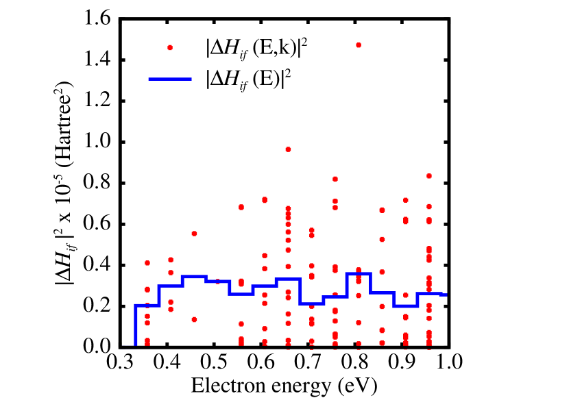
Figure 1: Calculated electronic matrix elements as a function of the initial state electron energy for a triply hydrogenated vacancy in Si with a bare dangling bond. Red points: matrix element values at each energy for different $k$ points; blue curve: Averaged matrix element over all $k$ points for each energy.

In Fig. 1, we show the values of calculated electronic matrix elements as a function of energy. At each energy value, there are a number of $k$ points that contribute. Their contributions are indicated by red symbols. The size of the energy bin is determined by the number of $k$ points. For the example shown in Fig. 1 the average matrix element as a function of energy is shown by the blue line. The size of the energy bin fixes the resolution. A smooth curve can only be obtained with very small energy bins, which requires a very large number of $k$ points. It is clear from the figure that the capture electronic matrix element is relatively constant as a function of energy, whereby it seems best at this point to take it to be a constant, either an average value or the value at the threshold for capture, which introduces an error bar of a factor of $\sim 1.7$ (clearly, to validate the theory against accurate experimental data, we need a very accurate calculation in the near-threshold region).

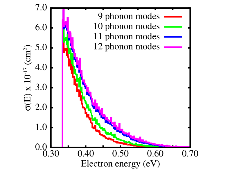
Figure 2: Calculated electron capture cross section using a constant electron matrix element and different number of phonon modes.

In Fig. 2, we show the calculated capture cross section using a constant matrix element to show clearly the convergence of the line-shape function as we increase the number of phonon modes that are used to construct configurations (the electronic matrix element is just a multiplier that sets the absolute value). The dominant contribution to the line-shape function comes from the balance between the modes with largest general coordinate displacement (GCD) and the growth of the number of allowed combinations with smaller GCD. Note that the curves are smooth because we employ millions of configurations at each energy and therefore we have very tiny energy bins. It is clear that a single-phonon-mode approximation would be very poor indeed. In Fig. 3 we show the convergence of the capture cross section at threshold (for electrons at the bottom of the conduction band), which is what is usually measured. Once more, it is clear that the single-phonon mode approximation would be inadequate.

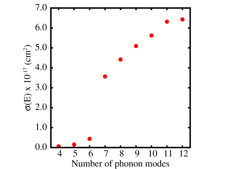
Figure 3: Convergence of the calculated electron capture cross section at the threshold as a function of the number of phonon modes.

For a calculation of the cross section using electronic matrix elements that depend on energy, the resolution is limited by the energy bin size. We show the result in Fig. 4. Clearly, the size of the energy bin is important. For capture cross sections, one is often interested only in the threshold value. The calculations presented here are a prelude to calculations of hot-electron inelastic multiphonon scattering, for which the energy dependence is important. The energy dependence is also important in luminescence curves, i.e., the classic Huang-Rhys problem that was treated in the single-phonon approximation in Ref. REF2012, (in the case of luminescence, MPPs dissipate only the relaxation energy of the defect, when one expects the phonon mode corresponding to the actual relaxation to dominate; nevertheless, a fully convergent calculation would be needed to establish the degree of accuracy one obtains with the single-mode approximation).

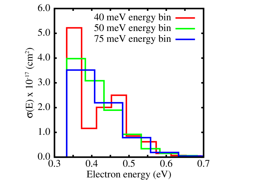
Figure 4: Calculated full capture cross section using the electron matrix element from Fig. 1 and 12 phonon modes in the line-shape function.

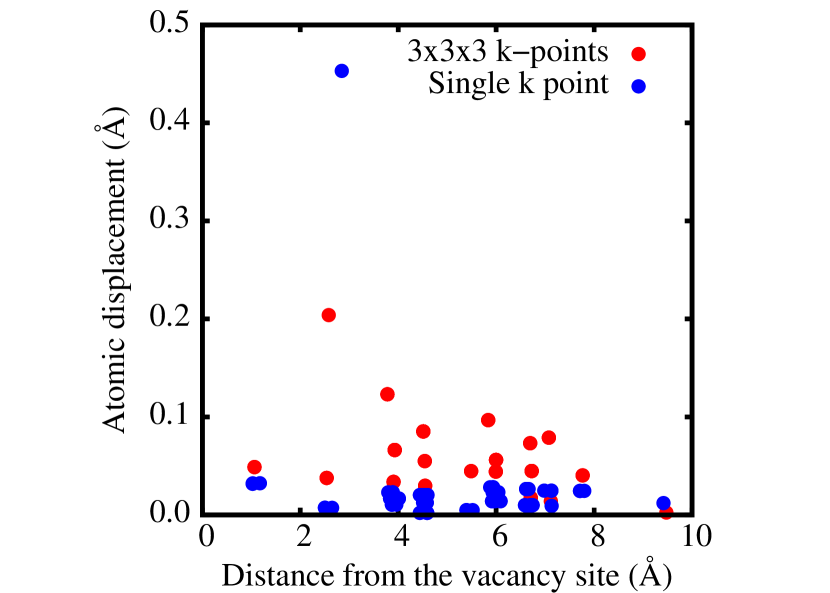
Figure 5: Atomic displacements of the triply-hydrogenated Si vacancy as a function of the distance from the vacancy site for a 64-atom supercell.

The accuracy of the calculation of the line shape function is controlled by the accuracy of the calculation of the generalized displacements. The latter depends on the accuracy of the calculation of the atomic displacements. We found that accuracy is enhanced significantly if we allow the entire supercell to relax, which allows the defect’s neighbors to relax more freely. At the same time, a dense $k$-point mesh is necessary. In Fig. 5, we present the atomic displacements of the triply-hydrogenated Si vacancy as a function of the distance from the vacancy site for a 64-atom supercell. Using only one $k$-point and not allowing the supercell to relax we get only the Si-atom near the defect to move significantly while the rest of the crystal remains essentially frozen (blue dots). This kind of relaxation leads to only a few phonon modes being significant and thus the system is artificially able to dissipate energy efficiently at certain frequencies. On the other hand the well-relaxed crystal of the ($3\times 3\times 3$) $k$-points grid (red dots) has more atoms contributing to the generalized displacements and thus almost all the phonon modes contribute in the dissipation to the energy of the incoming electron. The use of supercells with more than 64 atoms would be prohitively expensive for the line-shape function calculation.

VI Summary

We have presented a comprehesive theory of inelastic multiphonon carrier capture and scattering processes. We showed that, under non-equilibrium conditions, i.e., in the presence of currents or hot electrons, the defect potential is primarily responsible for capture throught a zeroth-order term in an expansion in terms of the atomic displacements (relaxation) that accompanies capture. These terms were not included in any prior theory. Instead, the focus has always been on the linear terms, which we showed here to be much smaller because they depend on the inverse of the mass of typical atoms in the defect complex. The linear terms are dominant only in the limit of thermal equilibrium. For the first time, we used accurate all-electron wave functions obtained by the PAW method for the electronic matrix elements and an accurate Monte Carlo scheme to sample random configurations of up to 12 distinct phonon modes for the line-shape functions to achieve convergence (a single-phonon-mode approximation has been standard in prior calculations). We presented results for a prototype defect. More accurate hybrid exchange-correlation functionals are needed to produce results that are accurate enough for comparison with experimental data. In addition, a reliable comparison with data can only be made with experimental measurements of capture cross sections simultaneously with the determination of the elastic mean-free-path and the capture mean-free-path, as they appear in Eq. (1).

Appendix A Evaluation of the electronic matrix element for BOA transition

In the basis of $|\Psi_{n}\rangle$, the unperturbed Hamiltonian $\tilde{H}^{0}$ is diagonal with eigenenergies $\epsilon_{n}$. The total electron Hamiltonian $H=\tilde{H}^{0}+H_{1}^{BO}$ has coupling terms only between states $|\Psi_{i}\rangle$ and $|\Psi_{f}\rangle$. We can, therefore, construct solutions of

$$(\tilde{H}^{0}+H_{1}^{BO})|\Phi\rangle=E|\Phi\rangle.$$ (67)

in the form $|\Phi\rangle=a|\Psi_{i}\rangle+b|\Psi_{f}\rangle,$ so that

$$\begin{pmatrix}\epsilon_{i}&\Delta H_{if}\\ \Delta H_{fi}&\epsilon_{f}\end{pmatrix}\begin{pmatrix}a\\ b\end{pmatrix}=E\begin{pmatrix}a\\ b\end{pmatrix}.$$ (68)

There are two sets of solutions,

$$E_{i(f)}=\frac{1}{2}\left[\epsilon_{i}+\epsilon_{f}\pm\sqrt{(\epsilon_{i}-\epsilon_{f})^{2}+4|\Delta H_{if}|^{2}}\right],$$ (69)

where state $i$ takes the $+$ sign and state $f$ take the $-$ sign, since $E_{i}>E_{f}$. The coefficients satisfy

$$\epsilon_{i}a_{i}+\Delta H_{if}b_{i}=E_{i}a_{i}$$ (70)

and

$$|a_{i}|^{2}+|b_{i}|^{2}=1.$$ (71)

There is an arbitrary phase factor within $a_{i}$. We can define a set of solution as,

$$a_{i}=b_{f}^{\ast}=\sqrt{\frac{1}{2}+\sqrt{\frac{1}{4}-\left|\frac{\Delta H_{if}}{E_{i}-E_{f}}\right|^{2}}}$$ (72)

and

$$b_{i}=-a_{f}^{\ast}=\frac{\Delta H_{if}}{E_{i}-E_{f}}\frac{1}{{\displaystyle\sqrt{\frac{1}{2}+\sqrt{\frac{1}{4}-\left|\frac{\Delta H_{if}}{E_{i}-E_{f}}\right|^{2}}}}}.$$ (73)

If we can compute the overlap integral $\langle\Phi_{f}|\Psi_{i}\rangle=a_{f}$, then we can solve for $|\Delta H_{if}|^{2}$ from $|a_{f}|^{2}$ and find,

$$|\Delta H_{if}|^{2}=\frac{|\langle\Phi_{f}|\Psi_{i}\rangle|^{2}-|\langle\Phi_{f}|\Psi_{i}\rangle|^{4}}{\left(1-2|\langle\Phi_{f}|\Psi_{i}\rangle|^{2}\right)^{2}}\epsilon_{if}^{2}.$$ (74)

To be consistent with the phase of Eq. (73), we have,

$$M_{e}^{BO}=\langle\Psi_{f}|H_{1}^{BO}|\Psi_{i}\rangle=\Delta H_{if}=-\frac{\sqrt{1-|\langle\Phi_{f}|\Psi_{i}\rangle|^{2}}}{1-2|\langle\Phi_{f}|\Psi_{i}\rangle|^{2}}\langle\Phi_{f}|\Psi_{i}\rangle\epsilon_{if}.$$ (75)

The wave function $|\Psi_{i}\rangle$ is related to that of a perfect crystal $|\Psi_{i}^{(0)}\rangle$ through a perturbation expansion,

$$|\Psi_{i}^{(0)}\rangle=|\Psi_{i}\rangle-\sum_{i^{\prime}\neq i,f}\frac{\langle\Psi_{i^{\prime}}|\Delta H|\Psi_{i}\rangle}{\epsilon_{i^{\prime}}-\epsilon_{i}}|\Psi_{i^{\prime}}\rangle.$$ (76)

Because $H_{1}$ has only nonzero elements between the states $|\Psi_{i}\rangle$ and $|\Psi_{f}\rangle$, for $j\neq i,f$, the wave functions $|\Psi_{j}\rangle=|\Phi_{j}\rangle$ so that $\langle\Phi_{f}|\Psi_{j}\rangle=0$. Thus, to first order in the defect potential,

$$\langle\Phi_{f}|\Psi_{i}\rangle=\langle\Phi_{f}|\Psi_{i}^{0}\rangle,$$ (77)

and, assuming that $|\langle\Phi_{f}|\Psi_{i}^{0}\rangle|\ll 1$, we arrive at Eq. (23), which simplifies the evaluation of the overlap integral.

Appendix B Evaluation of the gradient terms

Using the result in the previous section for the matrix element $M_{e}^{BO}$, we now calculate the gradient terms in Eq. (19), $\nabla_{\mathbf{R}_{k}}M_{e}^{BO}+\langle\Psi_{f}|\nabla_{\mathbf{R}_{k}}H_{e}|\Psi_{i}\rangle$. Neglecting higher order $|\langle\Phi_{f}|\Psi_{i}\rangle|^{2}$ terms, the first gradient term is,

$$\nabla_{\mathbf{R}_{k}}M_{e}^{BO} = -\left(\langle\nabla_{\mathbf{R}_{k}}\Phi_{f}|\Psi_{i}\rangle+\langle\Phi_{f}|\nabla_{\mathbf{R}_{k}}\Psi_{i}\rangle\right)\epsilon_{if}-\langle\Phi_{f}|\Psi_{i}\rangle\nabla_{\mathbf{R}_{k}}\epsilon_{if}$$ (78)

$$= -\left(\langle\nabla_{\mathbf{R}_{k}}\Phi_{f}|\Psi_{i}\rangle+\langle\Phi_{f}|\nabla_{\mathbf{R}_{k}}\Psi_{i}\rangle\right)\epsilon_{if}-\langle\Phi_{f}|\Psi_{i}\rangle\langle\Psi_{f}|\nabla_{\mathbf{R}_{k}}H_{0}|\Psi_{f}\rangle,$$

where in the last step we used the fact that $\nabla_{\mathbf{R}_{k}}\epsilon_{i}=0$ (the initial state is at equilibrium) and the Helmann-Feynman theorem for $\nabla_{\mathbf{R}_{k}}\epsilon_{f}$. From Eq. (16) we have,

$$|\nabla_{\mathbf{R}_{k}}\Psi_{i}\rangle=\sum_{i^{\prime}\neq i}\frac{\langle\Psi_{i^{\prime}}|\nabla_{\mathbf{R}_{k}}H_{e}|\Psi_{i}\rangle}{\epsilon_{i^{\prime}}-\epsilon_{i}}|\Psi_{i^{\prime}}\rangle,$$ (79)

where we used $\nabla_{\mathbf{R}_{k}}H_{el}=\nabla_{\mathbf{R}_{k}}H_{e}$. Because $|\Psi_{i^{\prime}}\rangle=|\Phi_{i^{\prime}}\rangle$ for $i^{\prime}\neq i,f$ and $\langle\Phi_{f}|\Psi_{f}\rangle=1+O(|\langle\Phi_{f}|\Psi_{i}\rangle|^{2})$, we have,

$$\langle\Phi_{f}|\nabla_{\mathbf{R}_{k}}\Psi_{i}\rangle=\frac{\langle\Psi_{f}|\nabla_{\mathbf{R}_{k}}H_{e}|\Psi_{i}\rangle}{\epsilon_{if}}\langle\Phi_{f}|\Psi_{f}\rangle=\frac{\langle\Psi_{f}|\nabla_{\mathbf{R}_{k}}H_{e}|\Psi_{i}\rangle}{\epsilon_{if}}.$$ (80)

Similarly,

$$\langle\nabla_{\mathbf{R}_{k}}\Phi_{f}|\Psi_{i}\rangle=-\frac{\langle\Phi_{f}|\nabla_{\mathbf{R}_{k}}H_{e}|\Phi_{i}\rangle}{\epsilon_{if}}\langle\Phi_{i}|\Psi_{i}\rangle=-\frac{\langle\Phi_{f}|\nabla_{\mathbf{R}_{k}}H_{e}|\Phi_{i}\rangle}{\epsilon_{if}}.$$ (81)

Combining these results and noting that $H_{1}^{BO}$ does not have diagonal components, we arrive at

$$\nabla_{\mathbf{R}_{k}}M_{e}^{BO}+\langle\Psi_{f}|\nabla_{\mathbf{R}_{k}}H|\Psi_{i}\rangle=\langle\Phi_{f}|\nabla_{\mathbf{R}_{k}}H|\Phi_{i}\rangle-\langle\Phi_{f}|\Psi_{i}\rangle\langle\Psi_{f}|\nabla_{\mathbf{R}_{k}}H|\Psi_{f}\rangle.$$ (82)

We can use Eq. (77) and approximate $|\Psi_{f}\rangle\approx|\Phi_{f}\rangle$ to get Eq. (24).

Appendix C Evaluation of the overlap integral within the PAW

Consider the problem of evaluating the overlap integral $\langle\Psi|\Phi\rangle$ between two wave functions from two different solids (e.g., one is a perfect crystal and the other contains a defect). Using the PAW expansion of the full wave functions:

$$|\Psi\rangle=|\tilde{\Psi}\rangle+|\Psi^{AE}\rangle_{a}-|\Psi^{PS}\rangle_{a},$$ (83)

where $|\tilde{\Psi}\rangle$ is the pseudo wave function and $|\Psi^{AE}\rangle_{a}$ and $|\Psi^{PS}\rangle_{a}$ are the atomic wave functions inside the augmentation sphere of each atom $a$, and similarly,

$$|\Phi\rangle=|\tilde{\Phi}\rangle+|\Phi^{AE}\rangle_{b}-|\Phi^{PS}\rangle_{b}.$$ (84)

Now, $\langle\Psi|\Phi\rangle$ is given as:

$$\langle\Psi|\Phi\rangle = \left(\langle\tilde{\Psi}|+_{a}\langle\Psi^{AE}|-_{a}\langle\Psi^{PS}|\right)\left(|\tilde{\Phi}\rangle+|\Phi^{AE}\rangle_{b}-|\Phi^{PS}\rangle_{b}\right)$$ (85)

$$= \langle\tilde{\Psi}|\tilde{\Phi}\rangle+\langle\tilde{\Psi}|\Phi^{AE}\rangle_{b}-\langle\tilde{\Psi}|\Phi^{PS}\rangle_{b}+_{a}\langle\Psi^{AE}|\tilde{\Phi}\rangle-_{a}\langle\Psi^{PS}|\tilde{\Phi}\rangle$$

$$+ \left({}_{a}\langle\Psi^{AE}|-_{a}\langle\Psi^{PS}|\right)\left(|\Phi^{AE}\rangle_{b}-|\Phi^{PS}\rangle_{b}\right).$$

The first term, $\langle\tilde{\Psi}|\tilde{\Phi}\rangle$, is the overlap of the pseudo wavefunctions and can be easily calculated since the pseudo wavefuntions are expanded in the same base set of plane waves.

In order to evaluate the terms $\langle\tilde{\Psi}|\Phi^{AE}\rangle_{b}-\langle\tilde{\Psi}|\Phi^{PS}\rangle_{b}$ and ${}_{a}\langle\Psi^{AE}|\tilde{\Phi}\rangle-_{a}\langle\Psi^{PS}|\tilde{\Phi}\rangle$, we make use of the unitary operators constructed by the projectors $|\tilde{p}\rangle$ and the pseudo atomic wavefunctions $|\tilde{\phi}\rangle$:

$$\sum_{b,i_{b}}|\tilde{p}_{i_{b}}^{b}\rangle\langle\tilde{\phi}_{i_{b}}^{b}|=1$$ (86)

and

$$\sum_{a,i_{a}}|\tilde{\phi}_{i_{a}}^{a}\rangle\langle\tilde{p}_{i_{a}}^{a}|=1$$ (87)

inside the augmentation sphere of each atom $b$ of the perfect crystal and each atom $a$ of the solid with the defect respectively. Thus:

$$\langle\tilde{\Psi}|\Phi^{AE}\rangle_{b}-\langle\tilde{\Psi}|\Phi^{PS}\rangle_{b} = \sum_{b,i_{b}}\left(\langle\tilde{\Psi}|\tilde{p}_{i_{b}}^{b}\rangle\langle\tilde{\phi}_{i_{b}}^{b}|\Phi^{AE}\rangle_{b}-\langle\tilde{\Psi}|\tilde{p}_{i_{b}}^{b}\rangle\langle\tilde{\phi}_{i_{b}}^{b}|\Phi^{PS}\rangle_{b}\right)$$ (88)

and

$${}_{a}\langle\Psi^{AE}|\tilde{\Phi}\rangle-_{a}\langle\Psi^{PS}|\tilde{\Phi}\rangle = \sum_{a,{i_{a}}}\left({}_{a}\langle\Psi^{AE}|\tilde{\phi}_{i_{a}}^{a}\rangle\langle\tilde{p}_{i_{a}}^{a}|\tilde{\Phi}\rangle-_{a}\langle\Psi^{PS}|\tilde{\phi}_{i_{a}}^{a}\rangle\langle\tilde{p}_{i_{a}}^{a}|\tilde{\Phi}\rangle\right)$$ (89)

Equations (88) and (89) ensure that in the case that if the two solids are identical, i.e. $|\tilde{\Psi}\rangle$ and $|\tilde{\Phi}\rangle$ are eigenstates of the same Hamiltonian and the augmentations spheres are identical, the one center expansion $\sum_{i}|\tilde{\phi}\rangle\langle\tilde{p}|\tilde{\Psi}\rangle$ of the pseudo wavefunction is identical to the pseudo wavefunction $|\tilde{\Psi}\rangle$ inside the augmentations sphere and

$$\langle\tilde{\Psi}_{f}|\Phi^{AE}\rangle-\langle\tilde{\Psi}|\Phi^{PS}\rangle=\langle\tilde{\Psi}^{PS}|\Phi^{AE}\rangle-\langle\tilde{\Psi}^{PS}|\Phi^{PS}\rangle.$$ (90)

To evaluate Eqs. (88) and (89), we need the projections of the pseudo wavefunctions of the first solid to the projectors of the atomic wavefunctions of the second solid, $\langle\tilde{\Psi}|\tilde{p}_{i_{b}}^{b}\rangle$, and vise versa for the projections $\langle\tilde{p}_{i_{a}}^{a}|\tilde{\Phi}\rangle$. This can be easily calculated since both the pseudo wavefunctions and the projectors are expanded in the same base set of plane waves.

The difficulty in evaluating the last term in Eq. (85) $\left({}_{a}\langle\Psi^{AE}|-_{a}\langle\Psi^{PS}|\right)\left(|\Phi^{AE}\rangle_{b}-|\Phi^{PS}\rangle_{b}\right)$ is that the cutoff spheres for the two wave functions are usually not identical. We can bypass this difficulty by evaluating the integral with the assistance of a complete set of plane waves $|\mathbf{k}\rangle$,

$$\left({}_{a}\langle\Psi^{AE}|-_{a}\langle\Psi^{PS}|\right)\left(|\Phi^{AE}\rangle_{b}-|\Phi_{i}^{PS}\rangle_{b}\right) = \sum_{\mathbf{k}}\left({}_{a}\langle\Psi^{AE}|-_{a}\langle\Psi^{PS}|\right)|\mathbf{k}\rangle\langle\mathbf{k}|\left(|\Phi^{AE}\rangle_{b}-|\Phi^{PS}\rangle_{b}\right)$$

$$= \sum_{\mathbf{k}}\left({}_{a}\langle\Psi^{AE}|\mathbf{k}\rangle-_{a}\langle\Psi^{PS}|\mathbf{k}\rangle\right)\left(\langle\mathbf{k}|\Phi^{AE}\rangle_{b}-\langle\mathbf{k}|\Phi^{PS}\rangle_{b}\right).$$

The plane waves can be expanded in either sphere as

$$e^{i\mathbf{k}\cdot\mathbf{r}}=4\pi\sum_{lm}i^{l}j_{l}(kr)Y_{lm}^{\ast}(\hat{\mathbf{k}})Y_{lm}(\hat{\mathbf{r}}).$$ (91)

and using,

$$|\mathbf{k}\rangle=\frac{1}{\sqrt{V}}e^{i\mathbf{k}\cdot\mathbf{r}},$$ (92)

the all-electron and the pseudo atomic wave functions is written as:

$$|\Phi^{AE}\rangle_{b}=\sum_{b,i_{b}}R_{b,i_{b}}^{AE}Y_{l_{b},m_{b}}\langle\tilde{p}_{b,i_{b}}|\tilde{\Phi}_{i}\rangle,$$ (93)

$$|\Phi^{PS}\rangle_{b}=\sum_{b,i_{b}}R_{b,i_{b}}^{PS}Y_{l_{b},m_{b}}\langle\tilde{p}_{b,i_{b}}|\tilde{\Phi}_{i}\rangle,$$ (94)

$${}_{a}\langle\Psi^{AE}|\mathbf{k}\rangle-_{a}\langle\Psi^{PS}|\mathbf{k}\rangle=\frac{4\pi}{\sqrt{V}}\sum_{a,i_{a}}\langle\tilde{\Psi}|\tilde{p}_{a,i_{a}}\rangle e^{i\mathbf{k}\cdot\mathbf{R_{a}}}i^{l_{a}}Y_{l_{a},m_{a}}^{\ast}(\hat{\mathbf{k}})\int_{0}^{r_{a}}j_{l_{a}}(kr)(R_{a,i_{a}}^{AE}-R_{a,i_{a}}^{PS})r^{2}dr,$$ (95)

and

$$\langle\mathbf{k}|\Phi^{AE}\rangle_{b}-\langle\mathbf{k}|\Phi^{PS}\rangle_{b}=\frac{4\pi}{\sqrt{V}}\sum_{b,i_{b}}\langle\tilde{p}_{b,i_{b}}|\tilde{\Phi}\rangle e^{-i\mathbf{k}\cdot\mathbf{R_{b}}}(-i)^{l_{b}}Y_{l_{b},m_{b}}(\hat{\mathbf{k}})\int_{0}^{r_{b}}j_{l_{b}}(kr)(R_{b,i_{b}}^{AE}-R_{b,i_{b}}^{PS})r^{2}dr,$$ (96)

Appendix D Phonon integrals

The overlap matrix between the initial and final states for the mode $j$ is,

$$\langle X_{n_{j}^{f}}(q_{j}+\delta q_{j})|X_{n_{j}^{i}}(q_{j})\rangle=\int X_{n_{j}+p_{j}}(q_{j}+\delta q_{j})X_{n_{j}}(q_{j})dq_{j}.$$ (97)

where $n_{j}^{i}=n_{j}$ and $n_{j}^{f}=n_{j}+p_{j}$.

For convenience, we drop the subscript $j$ for $n_{j}$ and $p_{j}$. Expanding $X_{n}(q_{j}+\delta q_{j})$ in terms of $\delta q_{j}$,

$$X_{n}(q_{j}+\delta q_{j})=\sum_{l}\frac{1}{l!}\frac{d^{l}X_{n}(q_{j})}{dq_{j}^{l}}\delta q_{j}^{l}.$$ (98)

Defining the raising and lowering operators

$$\hat{a}_{\pm}=\mp\sqrt{\frac{\hbar}{2\omega_{j}}}\frac{d}{dq_{j}}+\sqrt{\frac{\omega_{j}}{2\hbar}}q_{j},$$ (99)

we have,

$$\hat{a}_{+}X_{n}(q_{j})=\sqrt{n+1}X_{n+1}(q_{j}),$$ (100)

and

$$\hat{a}_{-}X_{n}(q_{j})=\sqrt{n}X_{n-1}(q_{j}).$$ (101)

Subtracting the two, we find,

$$\frac{d}{dq_{j}}X_{n}(q_{j})=\sqrt{\frac{\omega_{j}}{2\hbar}}(\hat{a}_{-}-\hat{a}_{+})X_{n}(q_{j})=\sqrt{\frac{n\omega_{j}}{2\hbar}}X_{n-1}(q_{j})-\sqrt{\frac{(n+1)\omega_{j}}{2\hbar}}X_{n+1}(q_{j}).$$ (102)

Using this recursive relation, we find that the lowest order term for $\int X_{n}(q_{j}+\delta q_{j})X_{n+k}(q_{j})dq_{j}$ is $\delta q_{j}^{|k|}$. Therefore, for small $\delta q{}_{j}$ only $k=\pm 1$ terms dominates. It means that each mode would at most emit or absorb a single phonon.

The result for the integrals are,

$$\int\frac{dX_{n}(q)}{dq}X_{n+1}(q)dq=-\sqrt{\frac{(n+1)\omega_{j}}{2\hbar}},$$ (103)

(note that this was incorrectly given as $-(\sqrt{\hbar m\omega/2})\sqrt{n+1}$ in Ref. Huang:1950, ), and,

$$\int\frac{dX_{n}(q)}{dq}X_{n-1}(q)dq=\sqrt{\frac{n\omega_{j}}{2\hbar}}.$$ (104)

For linear phonon matrix elements, we have,

$$q_{j}X_{n}(q_{j})=\sqrt{\frac{\hbar}{2\omega_{j}}}(\hat{a}_{-}+\hat{a}_{+})X_{n}(q_{j})=\sqrt{\frac{n\hbar}{2\omega_{j}}}X_{n-1}(q_{j})+\sqrt{\frac{(n+1)\hbar}{2\omega_{j}}}X_{n+1}(q_{j}).$$ (105)

The integrals needed are,

$$\int X_{n}(q)X_{n+1}(q)qdq=\sqrt{\frac{(n+1)\hbar}{2\omega_{j}}},$$ (106)

$$\int X_{n}(q)X_{n-1}(q)qdq=\sqrt{\frac{n\hbar}{2\omega_{j}}},$$ (107)

and,

$$\int\frac{dX_{n}(q)}{dq}X_{n}(q)qdq=-\frac{1}{2}.$$ (108)

Appendix E Line shape function

We first consider a single phonon band, i.e., all of the phonon modes $\omega_{j}=\omega(\mathbf{k}_{j})$ form a single continuous band described by wave vectors $\mathbf{k}_{j}$. Because of the Born-von-Karman periodic boundary condition, the phonon band is discretized into $N$ modes. Suppose that $s$ modes go down by one quantum and $s+p$ modes go up by one quantum. Then the line shape factor, Eq. (41) with $M=1$, contains contributions formed from the following products,

$$\left\{\prod_{j=1}^{N}t_{j}\right\}\left\{\prod_{k\in s}f_{k,-}\right\}\left\{\prod_{l\in s+p}f_{l+}\right\}\times$$

$$\times\delta\left(\sum_{l\in s+p}[n_{l}^{i}\hbar(\omega_{l}^{f}-\omega_{l}^{i})+\hbar\omega_{l}^{f}]+\sum_{k\in s}[n_{k}^{i}\hbar(\omega_{k}^{f}-\omega_{k}^{i})-\hbar\omega_{k}^{f}]+\sum_{m\ni\{s,s+p\}}n_{m}^{i}\hbar(\omega_{m}^{f}-\omega_{m}^{i})+\epsilon_{if}\right),$$

$$\left\{\prod_{j=1}^{N}t_{j}\right\}\left\{\prod_{k\in s}f_{k,-}\right\}\left\{\prod_{l\in s+p}f_{l+}\right\}\delta\left(\sum_{l\in s+p}\hbar\omega_{l}^{f}-\sum_{k\in s}\hbar\omega_{k}^{f}+\sum_{j=1}^{N}n_{j}^{i}\hbar(\omega_{j}^{f}-\omega_{j}^{i})+\epsilon_{if}\right),$$ (109)

where $\sum_{j=1}^{N}n_{j}^{i}\hbar(\omega_{j}^{f}-\omega_{j}^{i})$ is the energy difference because of the different phonon frequencies of the initial and final configuration of the defect and $t_{j}$, $f_{-}$, and $f_{+}$ are defined as:

$$t_{j} =\left|\int X_{n_{j}}(q_{j})X_{n_{j}}(q_{j}+\delta q_{j})dq_{j}\right|^{2}$$

$$f_{k,-} =\frac{{\displaystyle\left|\int X_{n_{k}}(q_{k})X_{n_{k}-1}(q_{k}+\delta q_{k})dq_{k}\right|^{2}}}{{\displaystyle\left|\int X_{n_{k}}(q_{k})X_{n_{k}}(q_{k}+\delta q_{k})dq_{k}\right|^{2}}}$$ (110)

$$f_{l,+} =\frac{{\displaystyle\left|\int X_{n_{l}}(q_{l})X_{n_{l}+1}(q_{l}+\delta q_{l})dq_{l}\right|^{2}}}{{\displaystyle\left|\int X_{n_{l}}(q_{l})X_{n_{l}}(q_{l}+\delta q_{l})dq_{l}\right|^{2}}}.$$

A naive way to sum over all possible configurations is to neglect the difference in the frequencies and apply the same counting method as Huang and Rhys Huang:1950 to write the configurational sum for all such combinations of phonons as,

$$\frac{1}{s!(s+p)!}\left\{\prod_{j=1}^{N}t_{j}\right\}\left\{\sum_{k=1}^{N}f_{k,-}\right\}^{s}\left\{\sum_{l=1}^{N}f_{k,+}\right\}^{s+p}\delta\left(\sum_{l\in s+p}\hbar\omega_{l}^{f}-\sum_{k\in s}\hbar\omega_{k}^{f}+\sum_{j=1}^{N}n_{j}^{i}\hbar(\omega_{j}^{f}-\omega_{j}^{i})+\epsilon_{if}\right).$$ (111)

This would not be correct if the frequencies are different for each mode. Furthermore, the summation over configurations for large $N$ is needed to integrate out the $\delta$ function. Therefore the $\delta$ function cannot be left outside the summations. Let us consider one term in the $\delta$ function at a time. Consider one the plus terms $\hbar\omega_{m}^{f}$ and insert the $\delta$ function into one of the summations,

$$\frac{1}{s!(s+p)!}\left\{\prod_{j=1}^{N}t\right\}\left\{\sum_{k=1}^{N}f_{k,-}\right\}^{s}\left\{\sum_{l=1}^{N}f_{k,+}\right\}^{s+p-1}$$

$$\sum_{m=1}^{N}\left\{f_{m,+}\delta\left(\hbar\omega_{m}^{f}+\sum_{l\in s+p-1}\hbar\omega_{l}^{f}-\sum_{k\in s}\hbar\omega_{k}^{f}+\sum_{j=1}^{N}n_{j}^{i}\hbar(\omega_{j}^{f}-\omega_{j}^{i})+\epsilon_{if}\right)\right\}.$$ (112)

For large $N$, each of the summations inside the curly brackets can be converted into integrals and evaluated,

$$S_{\pm}=\sum_{k=1}^{N}f_{k,\pm}=\frac{N}{\Omega_{\mathbf{k}}}\int f_{\mathbf{k},\pm}d\mathbf{k}=\begin{pmatrix}n+1\\ n\end{pmatrix}\frac{\omega}{2\hbar}N\delta q^{2},$$ (113)

where $\Omega_{\mathbf{k}}$ is the volume of the reciprocal space Brillouin zone. In the last step we assumed that the frequency and displacement do not change with $\mathbf{k}$.

In order to evaluated the last factor that includes the $\delta$ function, we note that each term in the summation over $m$ has a different $\omega_{m}^{f}$, which spans the entire phonon band when $m$ scans from $1$ to $N$. Thus as we convert the sum over $m$ to integral over $\mathbf{k}$, the argument $\omega_{m}^{f}$ is also converted to $\omega_{\mathbf{k}}$,

$$\sum_{m=1}^{N}\left\{f_{m,+}\delta\left(\hbar\omega_{m}^{f}+\sum_{l\in s+p-1}\hbar\omega_{l}^{f}-\sum_{k\in s}\hbar\omega_{k}^{f}+\sum_{j=1}^{N}n_{j}^{i}\hbar(\omega_{j}^{f}-\omega_{j}^{i})+\epsilon_{if}\right)\right\}$$

$$\approx\frac{N}{\Omega_{\mathbf{k}}}\int f_{\mathbf{k},+}\delta\left(\hbar\omega_{\mathbf{k}}^{f}+\sum_{l\in s+p-1}\hbar\omega_{l}^{f}-\sum_{k\in s}\hbar\omega_{k}^{f}+\sum_{j=1}^{N}n_{j}^{i}\hbar(\omega_{j}^{f}-\omega_{j}^{i})+\epsilon_{if}\right)d\mathbf{k}$$

$$=\left.S_{+}\frac{D(\omega)}{\Omega_{\mathbf{k}}}\right|_{\hbar\omega^{f}+\sum_{l\in s+p-1}\hbar\omega_{l}^{f}-\sum_{k\in s}\hbar\omega_{k}^{f}+\sum_{j=1}^{N}n_{j}^{i}\hbar(\omega_{j}^{f}-\omega_{j}^{i})+\epsilon_{if}=0},$$ (114)

where $D(\omega)$ is the phonon density of states. Combining the above equations and then setting all frequencies to $\omega$, Eq. (112) now becomes,

$$\frac{1}{s!(s+p)!}\left\{\prod_{j=1}^{N}t\right\}S_{-}^{s}S_{+}^{s+p}\left.\frac{D(\omega)}{\Omega_{\mathbf{k}}}\right|_{p\hbar\omega+\sum_{j=1}^{N}n_{j}^{i}\hbar(\omega_{j}^{f}-\omega_{j}^{i})+\epsilon_{if}=0}.$$ (115)

But there is one such contribution for each $\omega_{k}$ or $\omega_{l}$ in the $\delta$ function, regardless of the sign of the frequency. For $s$ modes subtracting a phonon and $s+p$ modes adding a phonon there are total $2s+p$ such contributions. We thus sum over all the terms and obtain,

$$\frac{2s+p}{s!(s+p)!}\left\{\prod_{j=1}^{N}t_{j}\right\}S_{-}^{s}S_{+}^{s+p}\left.\frac{D(\omega)}{\Omega_{\mathbf{k}}}\right|_{p\hbar\omega+\sum_{j=1}^{N}n_{j}^{i}\hbar(\omega_{j}^{f}-\omega_{j}^{i})+\epsilon_{if}=0}.$$ (116)

Finally, the factor $\prod_{j=1}^{N}t_{j}$ is,

$$\prod_{j=1}^{N}\left|\int X_{n_{j}}(q_{j})X_{n_{j}}(q_{j}+\delta q_{j})dq_{j}\right|^{2}=\left[1-\frac{(2n+1)\omega}{4\hbar}\delta q^{2}\right]^{2N}=\exp\left[-(S_{+}+S_{-})\right].$$ (117)

The line shape factor for a single phonon band is,

$$\left.\frac{D(\omega)}{\Omega_{\mathbf{k}}}\right|_{p\hbar\omega+\epsilon_{if}=0}\exp\left[-(S_{+}+S_{-})\right]\sum_{s=0}^{\infty}\frac{2s+p}{s!(s+p)!}S_{+}^{s+p}S_{-}^{s}$$ (118)

$$= \left.\frac{D(\omega)}{\Omega_{\mathbf{k}}}\right|_{p\hbar\omega+\epsilon_{if}=0}\exp\left[-(S_{+}+S_{-})\right]\left(\frac{S_{+}}{S_{-}}\right)^{p/2}\times$$

$$\left[pI_{p}\left(2\sqrt{S_{+}S_{-}}\right)+2\sqrt{S_{+}S_{-}}I_{p+1}\left(2\sqrt{S_{+}S_{-}}\right)\right].$$

To generalize the above expression to multiple phonon bands, the normalization factor must be evaluated with a summation over both the band index and the $\mathbf{k}$ points within each band. If we use $F_{j}$ to denote the factor for a band that adds net $p_{j}$ phonons, i.e.,

$$F_{j}=\sum_{s_{j}=0}^{\infty}\frac{1}{s_{j}!(s_{j}+p_{j})!}\left\{\prod_{m=1}^{N}t_{jm}\right\}\left\{\sum_{k=1}^{N}f_{jk,-}\right\}^{s_{j}}\left\{\sum_{l=1}^{N}f_{jl,+}\right\}^{s_{j}+p_{j}}$$ (119)

then in a similar manner as for the case of a single phonon band, $F_{j}$ is evaluated to be,

$$F_{j}=\left(\frac{n_{j}+1}{n_{j}}\right)^{p_{j}/2}\exp\left[-S_{j}(2n_{j}+1)\right]I_{p_{j}}\left[2S_{j}\sqrt{n_{j}(n_{j}+1)}\right].$$ (120)

Now we insert the $\delta$ function into the product of $F_{j}$ in the same manner as in the case of a single band to form the full line shape factor, one phonon band at a time. For now let us consider the case where all $p_{j}$’s are positive. We have,

$$\frac{\prod_{j=1}^{M}F_{j}}{F_{j^{\prime\prime}}}\sum_{s_{j^{\prime\prime}}=0}^{\infty}\frac{2s_{j^{\prime\prime}}+p_{j^{\prime\prime}}}{s_{j^{\prime\prime}}!(s_{j^{\prime\prime}}+p_{j^{\prime\prime}})!}\left\{\prod_{m=1}^{N}t_{j^{\prime\prime}m}\right\}\left\{\sum_{k=1}^{N}f_{j^{\prime\prime}k,-}\right\}^{s_{j^{\prime\prime}}}\left\{\sum_{l=1}^{N}f_{j^{\prime\prime}l,+}\right\}^{s_{j^{\prime\prime}}+p_{j^{\prime\prime}}-1}\times$$ (121)

$$\sum_{m=1}^{N}f_{j^{\prime\prime}m,+}\delta\left(\hbar\omega_{j^{\prime\prime}m}^{f}+\sum_{l\in s_{j^{\prime\prime}}+p_{j^{\prime\prime}}-1}\hbar\omega_{j^{\prime\prime}l}^{f}-\sum_{k\in s_{j^{\prime\prime}}}\hbar\omega_{j^{\prime\prime}k}^{f}+\sum_{l^{\prime}=1}^{N}n_{j^{\prime\prime}l^{\prime}}^{i}\hbar(\omega_{j^{\prime\prime}l^{\prime}}^{f}-\omega_{j^{\prime\prime}l^{\prime}}^{i})+\right.$$

$$\left.\sum_{j^{\prime}\neq j^{\prime\prime},l\in s_{j^{\prime}}+p_{j^{\prime}}}\hbar\omega_{j^{\prime}l}^{f}-\sum_{j^{\prime}\neq j^{\prime\prime},l\in s_{j^{\prime}}}\hbar\omega_{j^{\prime}l}^{f}+\sum_{j^{\prime}\neq j^{\prime\prime},k^{\prime}=1}^{N}n_{j^{\prime}k^{\prime}}^{i}\hbar(\omega_{j^{\prime}k^{\prime}}^{f}-\omega_{j^{\prime}k^{\prime}}^{i})+\epsilon_{if}\right)$$

$$= \left(\prod_{j=1}^{M}F_{j}\right)\left.\frac{D(\omega_{j^{\prime\prime}})}{\Omega_{\mathbf{k}}}\right|_{\sum_{j^{\prime}}p_{j^{\prime}}\hbar\omega_{j^{\prime}}+\sum_{j=1}^{Md}\sum_{l=1}^{N}n_{jl}^{i}\hbar(\omega_{jl}^{f}-\omega_{jl}^{i})+\epsilon_{if}=0}\times$$

$$\left\{p_{j^{\prime\prime}}+2S_{j^{\prime\prime}}\sqrt{n_{j^{\prime\prime}}(n_{j^{\prime\prime}}+1)}\frac{I_{p_{j^{\prime\prime}}+1}\left[2S_{j^{\prime\prime}}\sqrt{n_{j^{\prime\prime}}(n_{j^{\prime\prime}}+1)}\right]}{I_{p_{j^{\prime\prime}}}\left[2S_{j^{\prime\prime}}\sqrt{n_{j^{\prime\prime}}(n_{j^{\prime\prime}}+1)}\right]}\right\}.$$

where $j^{\prime\prime}$ is one of the phonon bands and we have used Eqs. (113) and (114). Summing over all possible $j^{\prime\prime}$ terms and with an additional summation over all configurations $\{p_{j}\}$, we find,

$$F=\frac{1}{\Omega_{\mathbf{k}}}\sum_{\{p_{j}\}}\left.\left\{\left(\prod_{j=1}^{M}F_{j}\right)\sum_{j=1}^{M}\left\{p_{j}+2S_{j}\sqrt{n_{j}(n_{j}+1)}\frac{I_{p_{j}+1}\left[2S_{j}\sqrt{n_{j}(n_{j}+1)}\right]}{I_{p_{j}}\left[2S_{j}\sqrt{n_{j}(n_{j}+1)}\right]}\right\}D(\omega_{j})\right\}\right|_{\sum_{j=1}^{M}p_{j}\hbar\omega_{j}+\epsilon_{if}=0}.$$ (122)

If some of the $p_{j}$’s are negative, we need to switch the roles of $S_{+}$ and $S_{-}$ following Ref. Huang:1950, . Redefining $s_{j}+p_{j}\to s_{j}$ and $s_{j}\to s_{j}-p_{j}$ in Eq. (121), the factor corresponding to $p_{j}$ becomes,

$$-p_{j}+2S_{j}\sqrt{n_{j}(n_{j}+1)}\frac{I_{-p_{j}+1}\left[2S_{j}\sqrt{n_{j}(n_{j}+1)}\right]}{I_{-p_{j}}\left[2S_{j}\sqrt{n_{j}(n_{j}+1)}\right]}$$ (123)

$$= p_{j}+2S_{j}\sqrt{n_{j}(n_{j}+1)}\frac{I_{p_{j}+1}\left[2S_{j}\sqrt{n_{j}(n_{j}+1)}\right]}{I_{p_{j}}\left[2S_{j}\sqrt{n_{j}(n_{j}+1)}\right]},$$

using the recurrence relation for the Bessel functions. Therefore Eq. (122) is valid for both positive and negative $p_{j}$’s. Applying thermodynamic average to the occupation numbers, $n_{j}$ is replaced by the Bose-Einstein distribution function,

$$n_{j}\to\frac{1}{\exp(\hbar\omega_{j}/kT)-1},$$ (124)

$$\frac{n_{j}+1}{n_{j}}\to\exp\left(\frac{\hbar\omega}{kT}\right),$$ (125)

$$2n_{j}+1\to\coth\left(\frac{\hbar\omega}{2kT}\right),$$ (126)

and

$$2\sqrt{n_{j}(n_{j}+1)}\to\frac{1}{\sinh(\hbar\omega/2kT)},$$ (127)

we obtain Eqs. (42) and (43).

References

• (1) M.H. Evans, X.-G. Zhang, J.D. Joannopoulos, and S.T. Pantelides, Phys. Rev. Lett. 95, 106802 (2005).
• (2) G. Hadjisavvas, L. Tsetseris, and S.T. Pantelides, IEEE Electron Dev. Lett. 28, 1018 (2007).
• (3) O. D. Restrepo, K. Varga, and S. T. Pantelides, Appl. Phys. Lett. 94, 212103 (2009).
• (4) D.J. DiMaria, J. Appl. Phys. 86, 2100 (1999).
• (5) D.J. DiMaria, J. Appl. Phys. 87, 8707 (2000).
• (6) G. Meneghesso, G. Verzellesi, F. Danesin, F. Rampazzo, A. Tazzoli, M. Meneghini, and E. Zanoni, IEEE Trans. Dev. Mater. Reliab. 8, 332 (2008).
• (7) S.T. Pantelides, Y. Puzyrev, X. Shen, T. Roy, S. DasGupta, B.R. Tuttle, D.M. Fleetwood, and R.D. Schrimpf, Microelectron. Eng. 90, 3 (2012).
• (8) X. Shen, S. DasGupta, R. Reed, R. Schrimpf, D. Fleetwood, and S. Pantelides, J. Appl. Phys. 108, 114505 (2010).
• (9) M. Meneghini, U. Zehnder, B. Hahn, G. Meneghesso, and E. Zanoni, IEEE Electron Dev. Lett. 30, 1051 (2009).
• (10) M. Igalson, P. Zabierowski, D. Prz?do, A. Urbaniak, M. Edoff, and W.N. Shafarman, Sol. Energy Mater. Sol. Cells 93, 1290 (2009).
• (11) K. Huang and A. Rhys, Proc. R. Soc. London, Ser. A 204, 406 (1950).
• (12) R. Kubo, Phys. Rev. 86, 929 (1952).
• (13) R. Kubo and Y. Toyozawa, Progr. Theor. Phys. 13 (1955).
• (14) H. Gummel and M. Lax, Annals of Phys. 2, 28 (1957).
• (15) A. Kovarskii, Soviet Phys. Solid State 4, 1200 (1962).
• (16) A. Kovarskii and E. P. Sinyasvskii, Soviet Phys. Solid State 4, 2345 (1963).
• (17) E. P. Sinyavskii and A. Kovarskii, Soviet Phys. Solid State 9, 1142 (1967).
• (18) C. H. Henry and D. V. Lang, Phys. Rev. B 15, 989 (1977).
• (19) B. K. Ridley, J. Phys. C: Solid State Phys. 11, 2323 (1978).
• (20) K. Huang, Scientia Sinica 24, 27 (1981).
• (21) E.V. Doktorov, I.A. Malkin, and V.I. Man’ko, J. Mol. Spectrosc. 64, 302 (1977).
• (22) Raffaele Borrelli and Andrea Peluso, J. Chem. Phys. 119, 8437 (2003).
• (23) Audrius Alkauskas, John L. Lyons, Daniel Steiauf, and Chris G. Van de Walle, Phys. Rev. Lett. 109, 267401 (2012).
• (24) Audrius Alkauskas, Qimin Yan, and Chris G. Van de Walle, Phys. Rev. B 90, 075202 (2014).
• (25) Volkhard May and Oliver Kühn, Charge and Energy Transfer Dynamics in Molecular Systems, Wiley-VCH, 2004.
• (26) N. S. Hush, J. Chem. Phys. 28, 962 (1958).
• (27) N. S. Hush, Trans. Faraday Soc. 57, 557 (1961).
• (28) P. E. Blöchl, Phys. Rev. B 50, 17953 (1994).
• (29) F. Schanovsky, W. Gos, and T. Grasser, J. Vac. Sci. Technol. B 29, 01A201-1 (2011).
• (30) D. B. Laks, G. F. Neumark, and S. T. Pantelides, Phys. Rev. B 42, 5176 (1990).