Do Magnetic Fields Destroy Black Hole Accretion Disk g-Modes?

Abstract

Diskoseismology, the theoretical study of normal mode oscillations in geometrically thin, optically thick accretion disks, is a strong candidate to explain some QPOs in the power spectra of many black hole X-ray binary systems. The existence of g-modes, presumably the most robust and visible of the modes, depends on general relativistic gravitational trapping in the hottest part of the disk. As the existence of the required cavity in the presence of magnetic fields has been put into doubt by theoretical calculations, we will explore in greater generality what the inclusion of magnetic fields has to say on the existence of g-modes. We use an analytical perturbative approach on the equations of MHD to assess the impact of such effects. Our main conclusion is that there appears to be no compelling reason to discard g-modes. In particular, the inclusion of a non-zero radial component of the magnetic field enables a broader scenario for cavity non-destruction, especially taking into account recent simulations’ saturation values for the magnetic field.

1 INTRODUCTION

There currently exists a rich structure in the power spectra observations of black hole X-ray binary systems, which includes high frequency (40–450 Hz) quasi-periodic oscillations (QPO). Relativistic diskoseismology, the formalism of normal-mode oscillations of geometrically thin, optically thick accretion disks, is a strong candidate to explain at least some of these QPOs. (For a review, see Wagoner 2008.)

Diskoseismology’s perturbative approach assumes that the effects of magnetic fields have been incorporated in the background equilibrium solution and works with fluid perturbations in which magnetic fields play no effective role. The objective of this paper is to study analytically the effects of including small magnetic fields on the oscillations described by relativistic diskoseismology.

Building on previous work (Fu & Lai 2009, hereafter FL), we use a local (WKB) analysis of the full MHD equations to examine how the magnetic field affects the physics of radial wave propagation. The main difference with FL is that we include all three components of the magnetic field, not just the vertical and toroidal cases separately. We do assume, however, that the toroidal magnetic field component $B_{\phi}$ is larger than the other components (using cylindrical coordinates $r$, $\phi$, $z$). This assumption is supported by simulations (see Table 1).

We show that diskoseismic g-modes are more resistant to magnetic-field disruption than previously thought.

2 RELATIVISTIC DISKOSEISMOLOGY AND GRAVITATIONAL TRAPPING

Within diskoseismology, some observed high-frequency oscillations in the outgoing radiation of black hole X-ray binary systems such as GRO J1655-40 are due to normal modes of adiabatic hydrodynamic perturbations. These modes are the result of gravitational driving and pressure restoring forces in a geometrically thin, optically thick accretion disc in the weak thermal, steep power-law state (Remillard & McClintock 2006).

The study of diskoseismology reveals the existence of different types of oscillation modes. Of these, the fundamental g-mode (an axisymmetric inertial-gravitational mode that oscillates mainly in the vertical plane) is the strongest candidate for explaining one of the QPOs, being the most robust and observable: it lies in the hottest part of the disk, has the largest photosphere, and is located away from the uncertain physics of the inner boundary (Perez et al. 1997). The p-modes, on the other hand, are less observable. They are only weakly affected by the magnetic fields (FL).

This interpretation is not only supported observationally by peaks in the power spectral density, but the g-mode has been observed in hydrodynamic simulations as well (Reynolds & Miller 2009; O’Neill, Reynolds, & Miller 2009).

As one can see in Fig. 1, the fundamental g-mode is trapped just under the maximum value of the radial epicyclic frequency $\kappa(r)$ in the absence of magnetic fields. Therefore, the existence of g-modes would be compromised by physical conditions that have an effect on the corresponding trapping curve. (The explanation of the other curves in the figure can be found in Section 4.)

3 THE EFFECTS OF INCLUDING MAGNETIC FIELDS

The inclusion of magnetic fields modifies the shape of the trapping curve in Fig. 1 and therefore threatens the existence of g-modes, given that it is not certain whether the inner boundary (the innermost stable circular orbit) can effectively trap this type of mode.

3.1 MHD Equations

The Newtonian ideal MHD equations for non-self-gravitating accretion disks are:

$$\frac{\partial\rho}{\partial t}+\nabla\cdot(\rho\mathbf{v})=0\,,$$ (1)

$$\frac{\partial\mathbf{v}}{\partial t}+(\mathbf{v}\cdot\nabla)\mathbf{v}=-\frac{1}{\rho}\nabla\Pi-\nabla\Phi+\frac{1}{\rho}\mathbf{T}\,,$$ (2)

$$\frac{\partial\mathbf{B}}{\partial t}=\nabla\times(\mathbf{v}\times\mathbf{B})\,,$$ (3)

with

$$\Pi\equiv P+\frac{B^{2}}{8\pi}\,,\qquad\mathbf{T}\equiv\frac{1}{4\pi}(\mathbf{B}\cdot\nabla)\mathbf{B}\,.$$ (4)

These are seven equations for seven unknowns: the density $\rho$, the velocity $\mathbf{v}$, and the magnetic field $\mathbf{B}$. A barotropic pressure $P=P(\rho)$ is assumed, $\Phi$ is the pseudo-Newtonian gravitational potential, and of course

$$\nabla\cdot\mathbf{B}=0\,.$$ (5)

We restrict our analysis to standard thin disks. We include the most important effects of general relativity by using the exact expressions for the orbital angular velocity $\Omega(r)$ and the radial epicyclic frequency $\kappa(r)$:

$$\Omega(r) = (r^{3/2}+a)^{-1}\,,$$ (6)

$$\kappa(r) = \Omega(r)(1-6/r+8a/r^{3/2}-3a^{2}/r^{2})^{1/2}\,.$$ (7)

There is then no need to specify $\Phi(r,z)$.

The standard approach includes the assumptions that the unperturbed background flow be axisymmetric, with $\mathbf{v}=r\Omega(r)\hat{\phi}$, and that $\mathbf{B}=B_{\phi}(r)\hat{\phi}+B_{z}\hat{z}$, where $B_{z}$ is a constant. These forms of $\mathbf{v}$ and $\mathbf{B}$ satisfy the stationary $(\partial/\partial t=0)$ equations (1) and (3). The radial force balance is dominated by the centrifugal and the gravitational terms, while the vertical balance is dominated by the vertical pressure gradient and the gravitational term. In other words, the magnetic fields are non-dominant.

3.2 Inclusion of Radial Magnetic Fields

In order to extend the usual approach, we include small (compared to $B_{\phi}$) radial magnetic fields. The traditional exclusion of radial magnetic fields in analytical treatments has no justification other than aesthetic prejudice (since they destroy the solutions’ stationarity). In fact, simulations consistently yield radial fields which are larger than vertical fields (see Table 1).

We now discuss what happens in the formalism once one introduces a radial $B_{r}\hat{r}$ term in the magnetic field of an otherwise stationary system, in particular the one described in the previous subsection. If this term has the form $B_{r}=C/r$, where $C$ is a constant, then (5) is immediately satisfied, while (3) yields:

$$B_{\phi}^{\rm new}=B_{\phi}^{\rm old}+\Delta B_{\phi}(r,t)\,,$$ (8)

where

$$\Delta B_{\phi}(r,t)\equiv rB_{r}\,\frac{d\Omega}{dr}\,t\,.$$ (9)

We note immediately that $\Delta B(r,t)\sim B_{r}\ll B_{\phi}$ for timescales of a few fluid oscillations (such that $\Omega t\sim 1$).

The new $B_{\phi}$ field satisfies equation (5), and (being parallel to $\mathbf{v}$) yields 0 on the right-hand side of equation (3).

In the context of the present paper on perturbations, we take $v_{r}$ as negligible. However, it is important to verify that such an assumption does not lead to inconsistencies at the unperturbed (equilibrium) level. The important point is that once one accepts a non-vanishing $B_{r}$, then one must allow for a non-zero $v_{r}$ in order to preserve the equality on equation (2); in particular, this equation acquires a $\phi$-component.

Fortunately, the implied value for $v_{r}\sim\varepsilon^{2}\,b_{r}^{2}\,r\Omega$ is in fact no larger than the one expected from standard (Novikov & Thorne 1973) viscosity considerations alone, which is $v_{r}\sim\varepsilon^{2}\alpha_{*}r\Omega$. Here, $\alpha_{*}$ is the “viscosity parameter” (shear stress/pressure),

$$\varepsilon\equiv\frac{h}{R}=\frac{\rm disk\ thickness}{{\rm typical\ value\ of\ }r}\,,$$ (10)

while $b_{r}$ is defined in equation (13).

3.3 Perturbations

We consider perturbations of $\delta\rho$, $\delta\mathbf{v}$, and $\delta\mathbf{B}\propto e^{im\phi-i\omega t}$. Recall that our unperturbed magnetic field has the form

$$\mathbf{B}=B_{\phi}(r)\hat{\phi}+(C/r)\hat{r}+B_{z}\hat{z}\,.$$ (11)

We work with the assumptions

$$B_{r}^{2},B_{z}^{2}\ll B_{\phi}^{2}\ll 4\pi P\sim 4\pi\rho c_{s}^{2}\,$$ (12)

(where $c_{s}$ refers to the speed of sound) and define the following small parameter:

$$b_{i}\equiv\frac{B_{i}}{\sqrt{4\pi\rho c_{s}^{2}}}=\frac{v_{Ai}}{c_{s}}\,\qquad(i=r,z,\phi)\,,$$ (13)

where $\mathbf{v}_{\!A}$ is the Alfvén velocity. The linearized equations for the perturbations then become:

$$-i\tilde{\omega}\delta\rho+\frac{1}{r}\frac{\partial}{\partial r}(\rho r\delta v_{r})+\frac{im\rho}{r}\delta v_{\phi}+\frac{\partial}{\partial z}(\rho\delta v_{z})=0\,,$$ (14)

$$-i\tilde{\omega}\delta v_{r}-2\Omega\delta v_{\phi}=G_{r}\frac{\delta\rho}{\rho}-\frac{1}{\rho}\frac{\partial}{\partial r}\delta\Pi\\ +\frac{1}{4\pi\rho}\left[\frac{im}{r}B_{\phi}+B_{z}\frac{\partial}{\partial z}{+B_{r}\frac{\partial}{\partial r}+\frac{\partial B_{r}}{\partial r}}\right]\delta B_{r}-\frac{B_{\phi}}{2\pi\rho r}\delta B_{\phi}\,,$$ (15)

$$-i\tilde{\omega}\delta v_{\phi}+\frac{\kappa^{2}}{2\Omega}\delta v_{r}={G_{\phi}\frac{\delta\rho}{\rho}}-\frac{im}{\rho r}\delta\Pi+\frac{1}{4\pi\rho}\left[\frac{im}{r}B_{\phi}+B_{z}\frac{\partial}{\partial z}{+B_{r}\left(\frac{\partial}{\partial r}+\frac{1}{r}\right)}\right]\delta B_{\phi}+\frac{1}{4\pi\rho}\left(\frac{B_{\phi}}{r}+\frac{\partial B_{\phi}}{\partial r}\right)\delta B_{r}\,,$$ (16)

$$-i\tilde{\omega}\delta v_{z}=G_{z}\frac{\delta\rho}{\rho}-\frac{1}{\rho}\frac{\partial}{\partial z}\delta\Pi+\frac{1}{4\pi\rho}\left[\frac{im}{r}B_{\phi}+B_{z}\frac{\partial}{\partial z}{+B_{r}\frac{\partial}{\partial r}}\right]\delta B_{z}\,,$$ (17)

$$-i\tilde{\omega}\delta B_{r}=\left(\frac{imB_{\phi}}{r}+B_{z}\frac{\partial}{\partial z}\right)\delta v_{r}{-\frac{imB_{r}}{r}\delta v_{\phi}-B_{r}\frac{\partial}{\partial z}\delta v_{z}}\,,$$ (18)

$$-i\tilde{\omega}\delta B_{\phi}=-\frac{\partial}{\partial r}(B_{\phi}\delta v_{r})+B_{z}\frac{\partial}{\partial z}\delta v_{\phi}-B_{\phi}\frac{\partial}{\partial z}\delta v_{z}{+\frac{\partial}{\partial r}(B_{r}\delta v_{\phi})}+r\frac{d\Omega}{dr}\delta B_{r}\,,$$ (19)

$$-i\tilde{\omega}\delta B_{z}=-\frac{B_{z}}{r}\frac{\partial}{\partial r}(r\delta v_{r})-\frac{imB_{z}}{r}\delta v_{\phi}+\left(\frac{imB_{\phi}}{r}{+B_{r}\frac{\partial}{\partial r}}\right)\delta v_{z}\,.$$ (20)

We have used the definitions $\tilde{\omega}\equiv\omega-m\Omega$ and

$$\mathbf{G}\equiv\frac{1}{\rho}\nabla\Pi-\frac{1}{\rho}\mathbf{T}\,.$$ (21)

3.4 WKB Analysis of Axisymmetric Oscillations

We now restrict ourselves to WKB conditions, in which by definition all perturbations are $\propto e^{ik_{r}r+ik_{z}z}$. Furthermore, we study for simplicity axisymmetric (i.e., $m=0$) oscillations, which are also more observationally relevant. We use $\delta\Pi$ instead of $\delta\rho$. Assuming $k_{r},k_{z}\gg 1/r$ and $B_{\phi}\propto r^{q}$, and using the definition $p\equiv d\ln\Omega/d\ln r$, the following equations obtain:

$$-\frac{i\omega}{\rho c_{s}^{2}}\delta\Pi+ik_{r}\delta v_{r}+ik_{z}\delta v_{z}+\frac{i\omega}{4\pi\rho c_{s}^{2}}(B_{\phi}\delta B_{\phi}{+B_{z}\delta B_{z}}{+B_{r}\delta B_{r}})=0\,,$$ (22)

$$-\frac{ik_{r}}{\rho}\delta\Pi+i\omega\delta v_{r}+2\Omega\delta v_{\phi}+\frac{1}{4\pi\rho}\left({ik_{z}B_{z}}{+ik_{r}B_{r}}\right)\delta B_{r}-\frac{B_{\phi}}{2\pi\rho r}\delta B_{\phi}=0\,,$$ (23)

$$i\omega\delta v_{\phi}-\frac{\kappa^{2}}{2\Omega}\delta v_{r}+\frac{1}{4\pi\rho}\left({ik_{z}B_{z}}{+ik_{r}B_{r}}\right)\delta B_{\phi}+\frac{(1+q)B_{\phi}}{4\pi\rho r}\delta B_{r}=0\,,$$ (24)

$$-\frac{ik_{z}}{\rho}\delta\Pi+i\omega\delta v_{z}+\frac{1}{4\pi\rho}\left({ik_{z}B_{z}}{+ik_{r}B_{r}}\right)\delta B_{z}=0\,,$$ (25)

$$ik_{z}B_{z}\delta v_{r}+i\omega\delta B_{r}{-ik_{z}B_{r}\delta v_{z}}=0\,,$$ (26)

$$ik_{r}B_{\phi}\delta v_{r}-\left({ik_{z}B_{z}}{+ik_{r}B_{r}}\right)\delta v_{\phi}+ik_{z}B_{\phi}\delta v_{z}-i\omega\delta B_{\phi}-p\Omega\delta B_{r}=0\,,$$ (27)

$${ik_{r}B_{z}\delta v_{r}}{-ik_{r}B_{r}\delta v_{z}}-i\omega\delta B_{z}=0\,.$$ (28)

The quantities $G_{z}$, $G_{\phi}$, and $G_{r}$ have been neglected. Being an odd function of $z$, $G_{z}$ is negligible near the midplane $z=0$, and goes away when vertically averaging. The fact that we are close to a purely axisymmetric configuration (as discussed above) implies that $G_{\phi}$ is also negligible for our purposes, whereas the term containing $G_{r}$ in equation (15) is smaller than the other ones because radial-force balance is dominated by the centrifugal and gravitational terms in thin disks.

4 CAVITY BEHAVIOR

In order to study the behavior of the g-mode trapping cavity under the inclusion of magnetic fields, one first obtains a dispersion relation from the equations for the perturbations derived in the previous subsection. Once the characteristic equation has been obtained, one needs to isolate the appropriate branch for $\omega$, which is the one that has $\kappa$ as its leading term when the magnetic field goes to zero. An exploratory way of doing this is working to zeroth-order in $k_{r}^{2}$ (i.e., setting $k_{r}^{2}=0$). The curves in Fig. 1 were obtained with this assumption, by means of a numerical approach (using the values for $b_{i}$ from Table 1). From now on we work with a non-zero $k_{r}^{2}$.

Before doing that, though, a word on dispersion relation branches. The branches that describe Alfvén waves and slow magnetosonic waves, which are the ones responsible for the magneto-rotational instability (MRI), are different ones from the one we study in this paper (Balbus & Hawley 1998). In particular, the MRI branches are characterized by low frequencies and growth rates of order $b_{z}^{1/2}\,\Omega$, which can be smaller than the g-mode frequencies. More explicitly, the typical timescale for MRI growth $\tau_{\rm MRI}$ is related to the g-mode oscillation period $\tau_{\rm g}$ by the following formula:

$$\frac{\tau_{\rm MRI}}{\tau_{\rm g}}\sim\frac{\kappa}{\Omega}\,b_{z}^{-1/2}\,,$$ (29)

which is $\sim 3$ for typical values of the involved quantities. Even though there are MRI effects of shorter timescales ($\sim 1/\Omega$), these only occur at very short length scales ($\ll$ disk thickness). Furthermore, the (alpha model) viscosity induced g-mode growth timescale $\tau_{\rm visc}$ (Ortega & Wagoner 2000) is related to $\tau_{\rm MRI}$ by:

$$\frac{\tau_{\rm MRI}}{\tau_{\rm visc}}\sim\frac{\alpha_{*}}{b_{z}^{1/2}}\,,$$ (30)

which means that the MRI might grow no faster than the viscous g-mode growth. These results indicate that the g-modes may survive in the presence of MRI driven turbulent eddies.

Another potential source of g-mode disruption is given by energy “pumping” from short to long length scales observed in freely decaying MHD turbulence, “inverse-cascade” simulations (Zrake 2014). On closer inspection, however, it is reassuring to see that the oscillation frequencies produced by this mechanism at the g-mode length scales are in reality much lower than the g-mode frequencies.

We now employ a perturbative approach in order to solve the problem. Recall that we work with the small quantities $\varepsilon\ll 1$ and $b_{z}^{2},b_{r}^{2}\ll b_{\phi}^{2}\ll 1$, and that we assume $m=0$.

The perturbed MHD equations (22)–(28), to order $b_{i}b_{j}$, lead to the relevant dispersion relation:

$$\omega=\omega_{0}+\Lambda b_{\phi}b_{z}+\lambda b_{\phi}b_{r}+\Gamma b_{z}^{2}+\gamma b_{r}^{2}+\beta b_{z}b_{r}\,,$$ (31)

where

$$[{\rm Re}(\omega_{0})]^{2} = \kappa^{2}-\frac{\kappa^{2}k_{r}^{2}c_{s}^{2}(1+b_{\phi}^{2})}{(k_{z}^{2}+k_{r}^{2})c_{s}^{2}(1+b_{\phi}^{2})-\kappa^{2}}\sim\kappa^{2}\,,$$ (32)

$${\rm Re(\Lambda)} = \frac{k_{z}^{3}c_{s}^{4}[\kappa^{2}+2(1-p+q)\Omega^{2}]}{2\Omega r\kappa^{2}(k_{z}^{2}c_{s}^{2}-\kappa^{2})}\sim\varepsilon\left(\frac{\Omega}{\kappa}\right)^{2}\Omega\,,$$ (33)

$${\rm Re(\lambda)} = \frac{(1-p+q)c_{s}^{2}\Omega k_{r}}{r\kappa^{2}}\sim\varepsilon^{3/2}\left(\frac{\Omega}{\kappa}\right)^{2}\Omega\,,$$ (34)

$${\rm Re(\Gamma)} = -\frac{p\Omega^{2}k_{z}^{2}c_{s}^{2}}{\kappa^{3}}\sim\left(\frac{\Omega}{\kappa}\right)^{3}\Omega\,,$$ (35)

$${\rm Re(\gamma)} = -\frac{p\Omega^{2}k_{r}^{2}c_{s}^{2}}{\kappa^{3}}\sim\varepsilon\left(\frac{\Omega}{\kappa}\right)^{3}\Omega\,,$$ (36)

$${\rm Re(\beta)} = \frac{2\Omega^{2}k_{r}k_{z}c_{s}^{2}}{\kappa^{3}}\sim\varepsilon^{1/2}\left(\frac{\Omega}{\kappa}\right)^{3}\Omega\,.$$ (37)

The leading imaginary contribution comes from the term

$${\rm Im(\Lambda)}=\frac{k_{z}k_{r}c_{s}^{2}[2(2+p)\Omega^{2}-\kappa^{2}]}{4\Omega(k_{z}^{2}c_{s}^{2}-\kappa^{2})}\sim\varepsilon^{1/2}\,\Omega\,,$$ (38)

the effects of which are small compared to the real-part terms. (We note that $\Omega^{2}\gg\kappa^{2}$ by one order of magnitude.)

We note that the implied inverse timescale for possible mode growth due to equation (38) is $1/\tau\sim b_{\phi}b_{z}\varepsilon^{1/2}\Omega$, which is much smaller than the one corresponding to purely viscous effects (no magnetic fields) on an fundamental g-mode, $1/\tau_{\rm visc}\sim\alpha_{*}\Omega$, except for very small values of $\alpha_{*}$.

We also note that the sign of Im($\Lambda$) is not determined by our formalism as $k_{r}$ and $k_{z}$ could have either values of the sign.

5 DISCUSSION

We are now in a position to offer an improved assessment of the effects on diskoseismology of finite magnetic fields, including the important radial magnetic fields.

Our results can be best appreciated in a plot of the form shown in Fig. 2, which describes the behavior of the trapping cavity in terms of the vertical and radial magnetic fields. The cavity is only destroyed (i.e., there is no value of the radius at which $d\omega(r)/dr$ vanishes) outside the corresponding ellipse, for sufficiently large $B_{z}$ and $B_{r}$ fields. This figure was obtained by scanning the behavior of $\omega(r)$ for different values of the $B_{i}$ and determining where the cavity disappears. (The mode lives in the range of radii where $k_{r}^{2}>0$ for a given eigenfrequency.)

In order to generate these results, the following ansatz was used: $k_{r}^{2}=\varepsilon k_{z}^{2}$, which is consistent with a radial mode size $\sim\sqrt{hR}$ [cf. eq. (5.1) in Perez et al. 1997], with $\varepsilon=0.1$, and $k_{z}^{2}c_{s}^{2}=\eta\Omega_{\perp}^{2}$ with $\eta=1$ (as in FL), where

$$\Omega_{\perp}(r)=\Omega(r)(1-4a/r^{3/2}+3a^{2}/r^{2})^{1/2}$$ (39)

is the vertical epicyclic frequency. In addition, we also used an alternative ansatz given by $k_{r}^{2}=\varepsilon^{2}k_{z}^{2}$, corresponding to a larger radial mode size $\sim R$, motivated by the fact that the g-mode radial extension might increase as the concavity of $\omega$ decreases. (This second ansatz gives the maximum radial g-mode extension that does not contradict the WKB assumption.)

Note that the dependence on $B_{\phi}$ is rather weak, as long as $B_{\phi}\gg B_{z},B_{r}$. Importantly, within each ellipse, the maximum value of $\omega(r)$ does not typically change by more than about $15\%$ (see Fig. 3 for a typical case), which means that the results are consistent with a constant QPO frequency within the present limits of observation. We should point out, however, that the numerical results of Fig. 1 imply a somewhat greater range of variation for the maximum value of $\omega$, in potential disagreement with observations. (Recall, though, that these results assume $k_{r}^{2}=0$.)

Even though the perturbative results cannot be directly compared to FL (who study only the $\mathbf{B}=B_{\phi}(r)\hat{\phi}$ and $\mathbf{B}=B_{z}\hat{z}$ special cases, separately), their results are consistent with ours in general terms.

Our main conclusions in the present exploratory approach are the following. First, from the above discussion there seems to be no compelling reason to discard axisymmetric g-mode $\kappa$ trapping. While it is still true that the inclusion of magnetic fields modifies the cavity, the situation is not as devastating as implied by FL. Note in particular that the inclusion of a non-zero $B_{r}$ potentially allows for slightly larger values of cavity-preserving $|B_{z}|$. Furthermore, the numerical results of Fig. 1 hint that the perturbative results may be underestimates of these $|B_{z}|$ values.

More importantly, most simulations appear to produce values of $B_{r}$ and $B_{z}$ which lie within or near each ellipse of Fig. 2. See Table 1 and corresponding bullets in Fig. 2. (Note, however, that there is an outlier point, not plotted.)

In the second place, it must be kept in mind that possible diskoseismic explanations of QPOs require only that the magnetic field be inside the ellipses in Fig. 2 during some, possibly small, fraction of the time, as the corresponding QPO duty cycles are observed to be much smaller than 100% (Remillard & McClintock 2006; Belloni, Sanna, & Méndez 2012).

Table 1: Saturation Values of the Magnetic Field.

Type of 3D Simulation	Initial $\mathbf{B}$ Field	$|b_{z}|$	$|b_{r}|$	$|b_{\phi}|$	Reference
shearing box, purely radial gravity	vertical	$<\,$0.09	$<\,$0.15	$<\,$0.26	1
shearing box, purely radial gravity	toroidal	$<\,$0.04	$<\,$0.07	$<\,$0.21	1
shearing box, purely radial gravity	$\langle\mathbf{B}\rangle=0$	$<\,$0.03	$<\,$0.05	$<\,$0.16	2
shearing box, including vertical gravity	twisted toroidal	$<\,$0.09	$<\,$0.11	$<\,$0.28	3
shearing box, including vertical gravity	vertical	$<\,$0.06	$<\,$0.08	$<\,$0.23	4
global, magnetically choked, $H/R\approx 0.5$	vertical	$<\,$0.08	$<\,$0.56	$<\,$0.56	5
global, $H/R=0.1$	toroidal	$<\,$0.05	$<\,$0.07	$<\,$0.17	6
global, different temperature profiles	vertical, weak	$<\,$0.04	$<\,$0.06	$<\,$0.17	7

Note. — Saturation values of the magnitude of the magnetic field components are quoted, in the form of $b_{i}\equiv v_{Ai}/c_{s}$, according to various 3D simulations. $H/R$ refers to the the disk’s typical thickness to radius ratio.

References. — (1) Hawley et al. 1995; (2) Hawley et al. 1996; (3) Shi et al. 2010; (4) Simon et al. 2011; (5) McKinney et al. 2012; (6) Parkin 2013; (7) Suzuki & Inutsuka 2014.

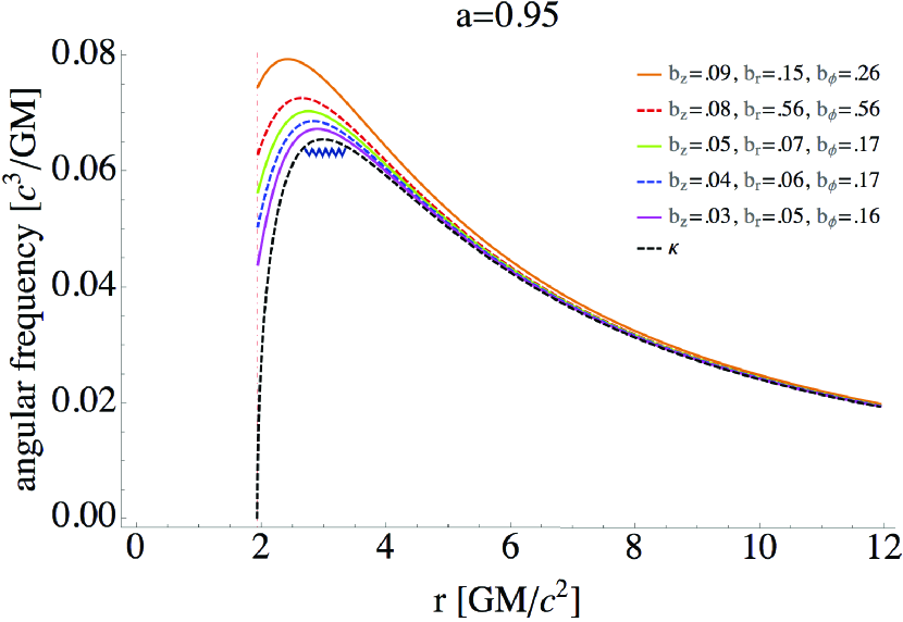
Figure 1: g-mode trapping cavity numerical estimates for different values of the magnetic field, assuming $m=0$ and setting $k_{r}=0$ as a first approximation (finite $k_{r}$ results within a perturbative approach are presented in Fig. 2 and discussed in Section 5). The normalized magnetic fields $b_{i}$ are defined in equation (13), and their values are taken from Table 1. (The listed $b_{i}$ values at the upper right corners correspond to the curves, in descending order.) For a given frequency, oscillating modes can exist below the corresponding curve. For high enough values of the magnetic field, the cavity is destroyed (not shown), i.e., the curve fails to have a maximum. Also shown is $\kappa(r)$, the leading term of the cavity in the absence of magnetic fields. Jagged curves are g-modes (shown here for the case of vanishing magnetic fields), dash-vertical lines mark the inner disk boundary at the ISCO. The upper and lower panels are for the respective cases of $a=0$ and $a=0.95$, where $a\equiv cJ/GM^{2}$ is the black hole angular momentum parameter. (This figure appears in color in the online version of the paper.)

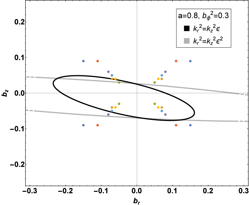
Figure 2: Behavior of the g-mode trapping cavity as a function of the three (normalized) components of the magnetic field $b_{i}$ for different values of $a$. The cavity is preserved within each ellipse (dark and light for $k_{r}^{2}=k_{z}^{2}\varepsilon$ and $k_{r}^{2}=k_{z}^{2}\varepsilon^{2}$, respectively, corresponding to different radial mode sizes), and destroyed outside it. Extrapolations to perturbative analysis are indicated by dashes; they occur whenever the maximum of $b_{r}^{2}$ and $b_{z}^{2}$ is larger than $b_{\phi}^{2}/4$. Also shown are bullets corresponding to Table 1 simulation saturation values (or their upper bounds), but note that we plot $\pm$ the values, as they carry no sign. We do not plot the outlier point. (This figure appears in color in the online version of the paper.)

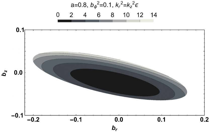
Figure 3: Behavior of the variation of the maximum value of $\omega$ within the (perturbative analysis) trapping-cavity ellipse for the case $a=0.8$, $b_{\phi}^{2}=0.1$, $k_{r}^{2}=k_{z}^{2}\varepsilon$ in Fig. 2, as a function of $b_{z}$ and $b_{r}$. Different shades of gray represent percentual differences, from 0% to 14%, with respect to the smallest maximum value. (See, however, the comment in the main text about the implications of the numerical results of Fig. 1.)

References

(1)
(2) Balbus, S. A., & Hawley, J. F. 1998,
Rev. Mod. Phys., 70, 1
(3)
(4) Belloni, T. M., Sanna, A., & Méndez, M. 2012,
MNRAS, 426, 1701
(5)
(6) Fu, W., & Lai, D. 2009, ApJ, 690, 1386 (FL)
(7)
(8) Hawley, J. F., Gammie, C. F., & Balbus, S. A. 1995, ApJ, 440, 742
(9)
(10) Hawley, J. F., Gammie, C. F., & Balbus, S. A. 1996, ApJ, 464, 690
(11)
(12) McKinney, J. C., Tchekhovskoy, A., & Blandford, R. D. 2012,
MNRAS, 423, 3083
(13)
(14) Novikov, I. D., & Thorne, K. S. 1973, in
Black Holes, ed. C. DeWitt & B. S. DeWitt
(New York : Gordon & Breach), 343
(15)
(16) O’Neill S. M., Reynolds C. S., & Miller C. M. 2009, ApJ, 693, 1100
(17)
(18) Ortega-Rodríguez, M., & Wagoner, R. V. 2000, ApJ, 537, 922
(19)
(20) Parkin, E. R. 2014, MNRAS, 441, 2078
(21)
(22) Perez, C. A., Silbergleit, A. S., Wagoner, R. V., & Lehr, D. E.
1997, ApJ, 476, 589
(23)
(24) Remillard, R. A., & McClintock, J. E. 2006,
Annu. Rev. Astron. Astrophys., 44, 49
(28) Shi, J., Krolik, J. H., & Hirose, S. 2010, ApJ, 708, 1716
(29)
(30) Simon, J. B., Hawley, J. F., & Beckwith, K. 2011,
ApJ, 730, 94
(31)
(32) Suzuki, T. K., & Inutsuka, S. I. 2014, ApJ, 784, 121
(33)
(34) Wagoner, R. V. 2008, New Astronomy Reviews, 51, 828
(35)
(36) Zrake, J. 2014, ApJ, 794, L26
(37)