Cosmological implications of different baryon acoustic oscillation data
Abstract
In this work, we explore the cosmological implications of different baryon acoustic oscillation (BAO) data, including the BAO data extracted by using the spherically averaged one-dimensional galaxy clustering (GC) statistics (hereafter BAO1) and the BAO data obtained by using the anisotropic two-dimensional GC statistics (hereafter BAO2). To make a comparison, we also take into account the case without BAO data (hereafter NO BAO). Firstly, making use of these BAO data, as well as the SNLS3 type Ia supernovae sample and the Planck distance priors data, we give the cosmological constraints of the CDM, the CDM, and the Chevallier-Polarski-Linder (CPL) model. Then, we discuss the impacts of different BAO data on cosmological consquences, including its effects on parameter space, equation of state (EoS), figure of merit (FoM), deceleration-acceleration transition redshift, Hubble parameter , deceleration parameter , statefinder hierarchy , and cosmic age . We find that: (1) NO BAO data always give a smallest fractional matter density , a largest fractional curvature density and a largest Hubble constant ; in contrast, BAO1 data always give a largest , a smallest and a smallest . (2) For the CDM and the CPL model, NO BAO data always give a largest EoS ; in contrast, BAO2 data always give a smallest . (3) Compared with the case of BAO1, BAO2 data always give a slightly larger FoM, and thus can give a cosmological constraint with a slightly better accuracy. (4) The impacts of different BAO data on the cosmic evolution and the comic age are very small, and can not be distinguished by using various dark energy diagnosis and the cosmic age data.
pacs:
98.80.-k, 98.80.Es, 95.36.+xI Introduction
Since its discovery in 1998 (Riess1998, ), cosmic acceleration has become one of the central problems in theoretical physics and modern cosmology. So far, we are still in the dark about the nature of this extremely counterintuitive phenomenon; it may be due to an unknown energy component, i.e., dark energy (DE), or a modification of general relativity, i.e., modified gravity (MG) (Caldwell2009, ).
One of the most powerful probes of DE is baryon acoustic oscillation (BAO), which can be used as a cosmological standard ruler to measure the expansion history of the Universe (Blake2003, ). The BAO scale can be measured in the power spectrum of cosmic microwave background (CMB) and in the maps of large-scale structure at lower redshifts. Moreover, for the latter, the BAO data can be extracted using either correlation function analysis (Eisenstein2005, ) or power spectrum analysis (Percival2010, ).
There are mainly two approaches to extract BAO scale from the galaxy redshift survey (GRS) data (Eisenstein2005, ; Tegmark2006, ; Percival2010, ; Padmanabhan2012, ; Anderson2012, ; Aubourg2014, ). The first approach is adopting the spherically averaged one-dimensional (1D) galaxy clustering (GC) statistics. For example, the BAO position in spherically averaged two point correlation functions (2PCF) provides a measure of an effective distance (Here denotes the redshift and denotes the speed of light), which was introduced by Eisenstein et al. (Eisenstein2005, ) according to the different dilation scales for the Hubble parameter and the angular diameter distance . Making using of the Sloan Digital Sky Survey Data Release 7 (SDSS DR7) (Abazajian2009, ), Padmanabhan et al. (Padmanabhan2012, ) gave ; based on the Baryon Oscillation Spectroscopic Survey Data Release 9 (BOSS DR9) (Eisenstein2011, ), Anderson et al. (Anderson2012, ) obtained . Here is the comoving sound horizon, and is the redshift of “drag” epoch when the baryons are “released” from the drag of the photons.
Another approach is making use of the anisotropic two-dimensional (2D) GC statistics. The key idea is separating the line of sight and transverse clustering so as to measure and separately (Okumura2008, ; anderson2014, ). In a series of works (ChuangWang, ), Chuang and Wang presented a method to obtain robust measurements of and simultaneously from the full 2D 2PCF. Applying this method to the BOSS DR9 data, Wang gave and . In addition, Hemantha, Wang and Chuang (Hemantha2014, ) also proposed a method to measure and simultaneously from the 2D matter power spectrum (MPS); applying this method to the SDSS DR7 sample, they obtained and .
Thus we have two types of BAO data: one is obtained by using the spherically averaged 1D GC statistics, another is obtained by using the anisotropic 2D GC statistics. An important difference between these two kinds of analyses is that the anisotropic analysis contains an Alcock-Paczynksi test (APtest1979, ). Although both these two types of BAO data are widely used in the literature to test various cosmological models (Addison2013, ; Aubourg2014, ), so far as we know, the effects of different BAO data on cosmology-fits and corresponding cosmological consequences have not been studied in the past. So the main aim of our work is presenting a comprehensive and systematic investigation on the cosmological implications of different BAO data. To make a comparison, we also take into account the case without any BAO data.
In this work, making use of these BAO data, as well as the SNLS3 type Ia supernovae (SNe Ia) data (Conley2011, ) and the Planck distance prior data (WangyunWangshuang2013, ), we constrain the parameter spaces of three simplest DE models, including the -cold-dark-matter (CDM) model, the CDM model, and the Chevallier-Polarski-Linder (CPL) model (Chevallier, ). Moreover, based on the fitting results, we study the impacts of different BAO data on cosmological consquences, including its effects on parameter space, equation of state (EoS) (MIDE1, ; MIDE2, ), figure of merit (FoM)(DETF2006, ; AB2007, ), deceleration-acceleration transition redshift, Hubble parameter , deceleration parameter , statefinder hierarchy and (ArabSahni2011, ), and cosmic age (Alcaniz and Lima, 1999).
II Methodology
In this section, firstly we review the theoretical framework of the DE models; then we describe the observational data used in the present work; finally we introduce the background knowledge about FoM, various DE diagnosis tools and cosmic age.
II.1 Theoretical Models
In a non-flat Universe, the Friedmann equation is
| (1) |
where is the Hubble parameter, is the scale factor of the Universe (we take today’s scale factor ), the dot denotes the derivative with respect to cosmic time , is the reduced Planck mass, is Newtonian gravitational constant, , , and are the energy densities of radiation, matter, spatial curvature and DE, respectively. The reduced Hubble parameter satisfies
| (2) |
where is the Hubble constant, , , and are the present fractional densities of radiation, matter, spatial curvature and DE, respectively. Per (WangWang2013, ), we take , where and . Since , is not an independent parameter (Zhangetal2012, ). Here the DE density function , which satisfies
| (3) |
where the EoS is the ratio of pressure to density for the DE
| (4) |
In the present work we just consider three simplest DE models:
-
•
CDM model, which has a cosmological constant (i.e. ). Then we have
(5) -
•
CDM model, which has a constant . Then we have
(6) -
•
CPL model (Chevallier, ) has a dynamical . Then we have
(7)
For each model, the expression of will be used to calculate the observational quantities appearing in the next subsection.
II.2 Observational Data
In this subsection, we describe the observational data used in this work.
II.2.1 BAO Data
In this work, we make use of two types of BAO data extracted from SDSS DR7 (Abazajian2009, ) and the BOSS DR9 (Eisenstein2011, ).
-
•
Let us introduce the BAO data obtained by using the spherically averaged 1D galaxy clustering statistics first. As mentioned above, making using of the SDSS DR7, Padmanabhan et al. (Padmanabhan2012, ) gave
(8) based on the BOSS DR9, Anderson et al. (Anderson2012, ) obtained
(9) The effective distance is given by (Eisenstein2005, ),
(10) where the angular diameter distance
(11) and the comoving distance
(12) Here , , , for , , and , respectively. In addition, the comoving sound horizon is given by (WangWang2013, )
(13) where , and is the present fractional density of baryon. The redshift of the drag epoch is well approximated by EisensteinHu1998
(14) where
(15) These BAO data are included in our analysis by adding , with and , to the of a given model. Then we have
(16) where is the standard deviation of data, , and . For simplicity, hereafter we will call this type BAO data “BAO1”.
-
•
Then, let us introduce the BAO data obtained by using the anisotropic 2D galaxy clustering statistics. Making use of the 2D MPS of SDSS DR7 samples, Hemantha, Wang, and Chuang (Hemantha2014, ) got
(17) In addition, using the 2D 2PCF of BOSS DR9 samples, Wang Wangyun2014 obtained
(18) These BAO data are included in our analysis by adding , with and , to the of a given model. Now we have
(19) where , , and . Based on Refs. (Hemantha2014, ) and (Wangyun2014, ), we get
(20) (21) For simplicity, hereafter we will call this type BAO data “BAO2”.
II.2.2 SNe Ia Data
For the SNe Ia data, we use the SNLS3 “combined” sample (Conley2011, ), which consisting of 472 SNe Ia. The function for the supernova (SN) data is given by
| (22) |
where is a vector of model residuals of the SN sample, and is the rest-frame peak band magnitude of the SN. The total covariance matrix C can be written as (Conley2011, )
| (23) |
Here denotes the diagonal part of the statistical uncertainty, and denote the statistical and systematic covariance matrices, respectively. For the details of constructing the covariance matrix C, see Conley2011 .
Current studies have found the evidence for the potential SN evolution. For examples, the studies on the SNLS3 (WangWang2013, ), the Union2.1 (Mohlabeng2013, ), the Pan-STARRS1 (Scolnic2014, ), and the JLA data sets (jlapotential, ) all indicated that, although the SN stretch-luminosity parameter is still consistent with a constant, the SN color-luminosity parameter evolves along with redshift at very high confidence level (CL). Moreover, this conclusion has significant effects on parameter estimation of various cosmological models (WLZ2014, ). Therefore, in the present work we adopt a constant and a linear , now the predicted magnitude of SN becomes 111It should be mentioned that, the intrinsic scatter also has the hint of redshift-dependence (Marrinerl2011, ) that will significantly affect the results of cosmology-fits. In addition, different light-curve fitters of SN can also affect the results of parameter estimation (Bengochea2011, ; HLLW2015, ). But in this work, we do not consider these factors for simplicity.
| (24) |
The luminosity distance is defined as
| (25) |
where and are the CMB restframe and heliocentric redshifts of SN, and has been given in Eq. (12). In addition, and are stretch measure and color measure for the SN light curve, is a parameter representing some combination of the absolute magnitude of a fiducial SNe Ia and the Hubble constant .
It must be emphasized that, in order to include host-galaxy information in the cosmological fits, Conley et al. (Conley2011, ) split the SNLS3 sample based on host-galaxy stellar mass at , and made to be different for the two samples. So there are two values of (i.e. and ) for the SNLS3 data. Moreover, Conley et al. removed and from cosmology-fits by analytically marginalizing over them (for more details, see the appendix C of (Conley2011, )). In the present work, we just follow the recipe of (Conley2011, ), and do not treat as model parameter. For simplicity, hereafter we will call this SNe Ia sample “SNLS3”.
II.2.3 CMB Data
For cosmic microwave background (CMB) data, we use the Planck distance priors data extracted from Planck first data release (WangyunWangshuang2013, ). CMB gives us the comoving distance to the photon-decoupling surface and the comoving sound horizon at photon-decoupling epoch . Wang and Mukherjee WangMukherjee2007 showed that the CMB shift parameters
| (26) |
together with , provide an efficient summary of CMB data as far as dark energy constraints go. Notice that is given in Eq. (12), is given in Eq. 13, and is given in Ref. (HuSugiyama1996, ). In (Li2008, ), Li et al. proved that CMB distance priors data can give similar constraints on DE parameters compared with the full CMB power spectrum data. This conclusion is also consistent with the result of (LiYH13, ), in which the holographic DE model is adopted in the background. Therefore, the use of the Planck distance prior is sufficient for our purpose.
Using the Planck+lensing+WP data, the mean values and 1 errors of are obtained (WangyunWangshuang2013, ),
| (27) |
Defining , , and , the normalized covariance matrix can be written as (WangyunWangshuang2013, )
| (28) |
Then, the covariance matrix for is given by
| (29) |
where . The CMB data are included in our analysis by adding the following term to the function:
| (30) |
where are the mean values from Eq. (27). For simplicity, hereafter we will call this CMB data “Planck”.
II.2.4 Total function
Now the total function is
| (31) |
We perform an MCMC likelihood analysis using the “CosmoMC” package (Lewis2002, ).
II.3 Figure of Merit, Dark Energy Diagnosis and Cosmic Age
Let us start from the FoM of DE. FoM was firstly proposed to make a comparison for different DE experiments. Making use of the CPL model, Dark Energy Task Force (DETF) developed a quantitive FoM to be the reciprocal of the area enclosed by the CL contour in the plane, satisfies (DETF2006, )
| (32) |
where , and . Note that , thus the conversion to is not needed to calculate the FoM. Soon after, various FoM quantities were proposed (AB2007, ). In this work, we just use the DETF version of FoM to make a comparison between different BAO data. It is clear that a larger indicates a better accuracy.
Then let us turn to various DE diagnosis. The scale factor of the Universe can be Taylor expanded around today’s cosmic age as follows:
| (33) |
where
| (34) |
with . The Hubble parameter contains the information of the first derivative of . Based on the BAO measurements from the BOSS DR9 and DR 11, Samushia et al. (Samushia2013, ) gave , while Delubac et al. (Delubac2015, ) obtained . These two H(z) data points will be used to compare the theoretical predictions of DE models.
In addition, the deceleration parameter is
| (35) |
which contains the information of the second derivatives of . It is clear that the expansion of the Universe underwent a transition from the deceleration phase to the acceleration phase in the past. The deceleration-acceleration transition redshift can be calculate using the condition
| (36) |
Lima et al. (Lima2012, ) argued that may be tightly constrained by ongoing and future observations. So it is interesting to check the impacts of different BAO data on the transition redshift .
The statefinder hierarchy, , is defined as (ArabSahni2011, ):
| (37) | |||
| (38) | |||
| (39) |
The reason for this redefinition is to peg the statefinder at unity for CDM during the cosmic expansion,
| (40) |
This equation defines a series of null diagnostics for CDM when . By using this diagnostic, we can easily distinguish the CDM model from other DE models. Because of , when , statefinder hierarchy can be rewritten as:
| (41) | |||
| (42) |
where the superscript is to discriminate between and . In this work, we use the statefinder hierarchy and to diagnose the impacts of different types BAO data on the three DE models.
At last, we introduce the cosmic age. The age of the Universe at redshift is given by
| (43) |
In history, the cosmic age problem played an important role in the cosmology Alcaniz and Lima (1999). Obviously, the age of the Universe at any redshift cannot be younger than its constituents at the same redshift. In the literature, some old high redshift objects (OHRO) have been considered extensively. For instance, the 3.5Gyr old galaxy LBDS 53W091 at redshift Dunlop et al. (1996), the 4.0Gyr old galaxy LBDS 53W069 at redshift Dunlop (1999), and the 2.0Gyr old quasar APM 08279+5255 at redshift Hasinger, Schartel, & Komossa (2002). The age data of these three OHRO (i.e. , and ) have been extensively used to test various cosmological models in the literature (see e.g. Alcaniz03 ).
III Results
III.1 Cosmology Fits and Corresponding Cosmological Consequences
In this subsection, we present the fitting results of the three DE models, and discuss the impacts of different BAO data on parameter estimation and FoM. For comparison, we also take into account the case without using BAO data. Hereafter, “NO BAO”, “BAO1” and “BAO2” represent the , the and the data, respectively.
| CDM | CDM | CPL | |||||||||
|---|---|---|---|---|---|---|---|---|---|---|---|
| Parameter | NO BAO | BAO1 | BAO2 | NO BAO | BAO1 | BAO2 | NO BAO | BAO1 | BAO2 | ||
In table 1, we list the cosmological fitting results for the CDM, the CDM and the CPL model. From this table we see that, for all the three DE models, including the BAO data in the analysis can remarkbly improve the fitting results. After making use of the BAO data, we see that for the CDM and the CDM model, the result of is consistent with the case of a spatially flat universe at CL, which is consistent with the results of pervious studies (Padmanabhan2012, ; Anderson2012, ; Sanchez2014, ; Planck201513, ) 222For example, the Planck group (Planck201513, ) investigated a non-flat CDM model, and found that .; in contrast, for the CPL model, both the result of given by BAO1 and BAO2 deviates from a spatially flat universe at CL, showing that there is a strong degeneracy between the evolution of EoS and the spatial curvature (CCB2007, ). Moreover, we find that among these three datasets, NO BAO data always give a smallest fractional matter density , a largest fractional curvature density and a largest Hubble constant ; in contrast, BAO1 data always give a largest , a smallest and a smallest . Since these results hold true for all the three DE models, we can conclude that our conclusion is insensitive to the DE considered in the background.
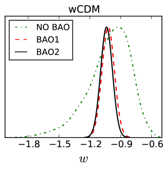
Let us discuss the issues of EoS in details. In Fig. 1, we plot the 1D marginalized probability distributions of for the CDM model. We see that, compared with the case without BAO data, adding BAO data in the analysis will yield a much smaller ; in other words, using BAO data will yield a best-fit result , while NO BAO data will lead to a best-fit result . Besides, making use of BAO data will also significantly reduce the error bar of , which corresponds to a better accuracy in parameter estimation. Moreover, we find that between these two types of BAO data, BAO2 data gives a slightly smaller , as well as a slightly smaller error bar of .
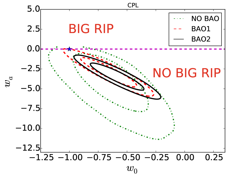
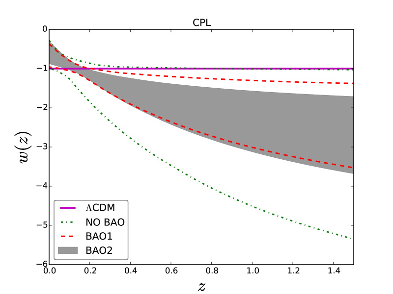
In the Fig. 2, we give a detailed analysis on the EoS of the CPL model. The left panel of Fig. 2 shows the 2D probability contours of at 1 and 2 CL. We see that, compared with the case of NO BAO, both BAO1 and BAO2 correspond to a significantly tighter 2D contours of , which implies that adding BAO data can significantly improve the fitting results. In addition, the fixed point = of the CDM model is located at the edge of CL contour given by the BAO1 data, but lies outside the CL contour given by the BAO2 data. This means that the result of BAO1 is closer to the CDM model. The right panel of Fig. 2 shows the confidence regions of in the redshift range . From this figure we see that, between the two types of BAO data, BAO2 yields a slightly smaller .
| Data | NO BAO | BAO1 | BAO2 |
|---|---|---|---|
Table 2 gives the results of for the CPL model. From this table we can see that, compared to the case of NO BAO, both the BAO1 and the BAO2 data give a much large value of : adding BAO1 will increase the value of by a factor of , while adding BAO2 will increase the value of by a factor of . This result shows the importance of using BAO measurements in measuring the cosmic expansion history and testing DE models. In addition, for the two types of BAO data, BAO2 can yield a slightly larger . This implies that the BAO2 data can give a fitting result with a slightly better accuracy.
III.2 Various DE Diagnosis and Cosmic Age
In this subsection, we study the impacts of different BAO data on the cosmic evolutions of various DE diagnosis (including , , and ) and the cosmic age .
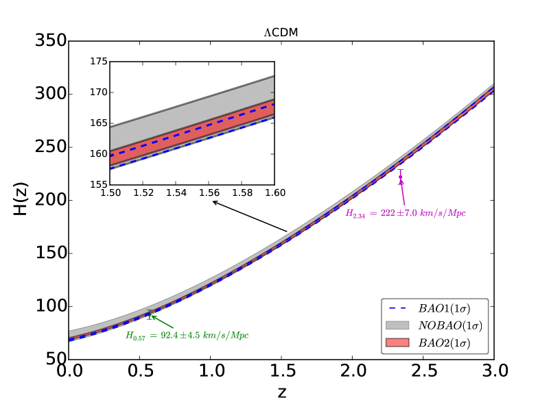
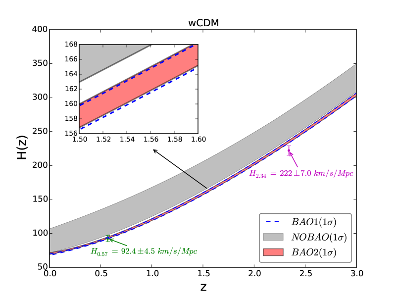
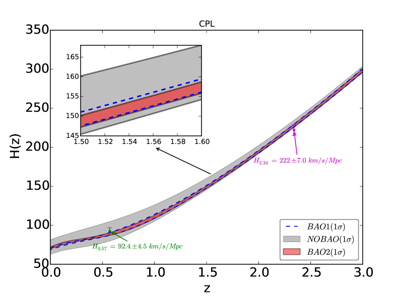
Fig. 3 shows the 1 confidence regions of Hubble parameter at redshift region for the three DE models. For comparison, two data points, and , are also marked by diamonds with error bars in this figure 333In fact, there actually exist a lot of other measurements. see e.g. (Ding2015, ). It can be seen that for the CDM model, the 1 confidence regions of given by NO BAO seperate from the results given by BAO1 and BAO2. This means that for the CDM model, adding BAO data in the analysis will yield quite different compared with the case without BAO data. After adding BAO data in the analysis, we find that the data point can be easily accommodated in all the three DE models. On the other side, the data point significantly deviates from the 1 regions of in the CDM and the CDM model, but it can be accommodated in the CPL model. This means that the tension between and other cosmological observations (Sahni2014, ) can be reduced by considering the evolution of EoS . In addition, the 1 confidence regions of given by different BAO data are almost overlap, this means that using diagram has great difficulty to distinguish the differences between the BAO1 and the BAO2 data.
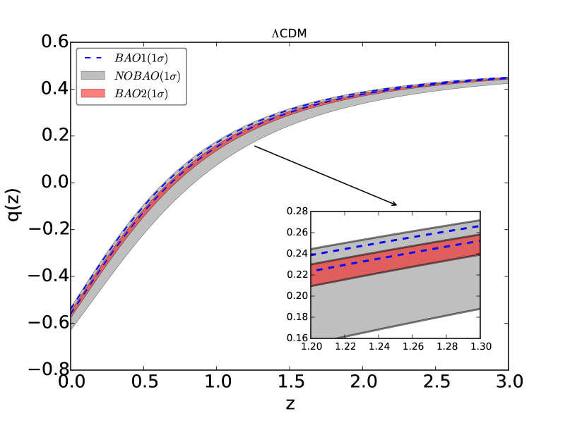
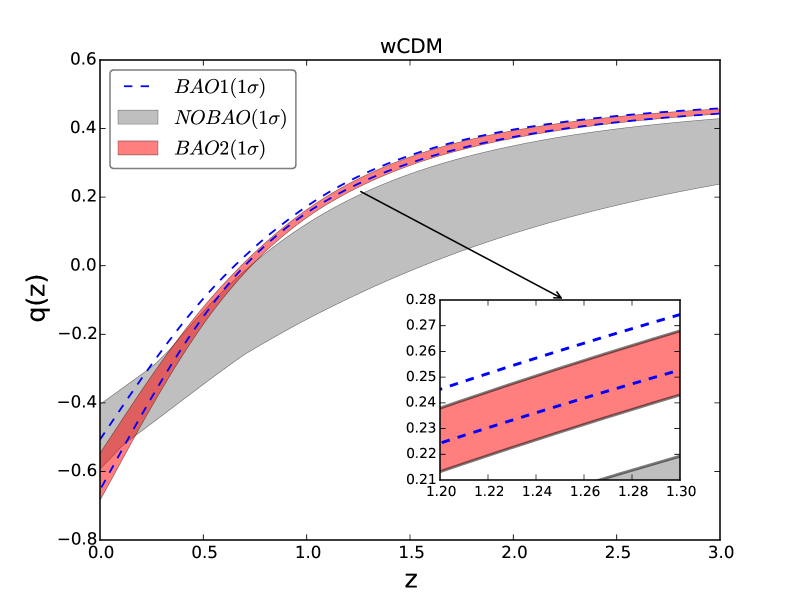
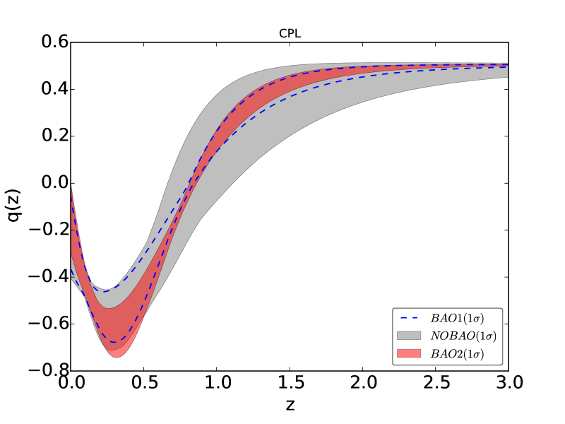
We plot the 1 confidence regions of deceleration parameter at redshift region in Fig. 4. From this figure we see that for the CDM model, using BAO data will yield quite different compared with the case without BAO data. In addition, we find that for the CPL model, achieves its minimum at , then starts to increase along with the decrease of redshift . This means that the current cosmic acceleration is probably slowing down. In fact, the possibility of a slowing down cosmic acceleration has been proposed by Shafieloo et al. in (Shafieloo2009, ); and in a recent work (YH2015, ), we have proved that this extremly counterintuitive phenomenon is insensitive to the specific form of . Moreover, for all the three models, we see that the 1 confidence regions of given by different BAO data are almost overlap, which implies that using diagram still has difficulty to distinguish the differences between the BAO1 and the BAO2 data.
| CDM | CDM | CPL | ||||||
| Quantity | BAO1 | BAO2 | BAO1 | BAO2 | BAO1 | BAO2 | ||
In table 3, we list the best fit values of deceleration-acceleration transition redshift for the three DE models. From this table we see that, for all the cases, the transition redshifts are located at mediate redshift (), which is consistent with the previous studies (Turner2002, ; Lima2012, ). Among the three DE models, the CDM model corresponds to a smaller , and the CPL model corresponds to a larger . In addition, for the two types of BAO data, BAO2 data always give a larger .
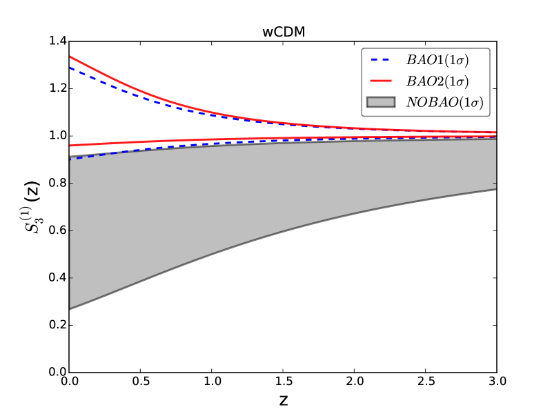
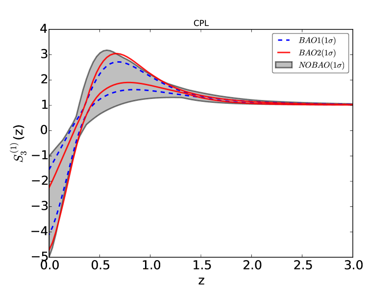
In Fig. 5, we plot the 1 confidence regions of statefinder hierarchy at redshift region [0,3] for the CDM model and the CPL model. From this figure we see that the evolution trajectory of given by the CDM model is quite different from the result of the CPL model, which has a peak at . This means that the statefinder hierarchy is a powerful tool that has the ability to distinguish different DE models. Moreover, we see that most of the 1 confidence regions of given by the two BAO data are overlap. This means that the statefinder still does not have the ability to distinguish the effects of different BAO data.
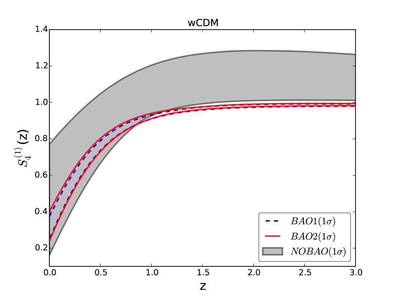
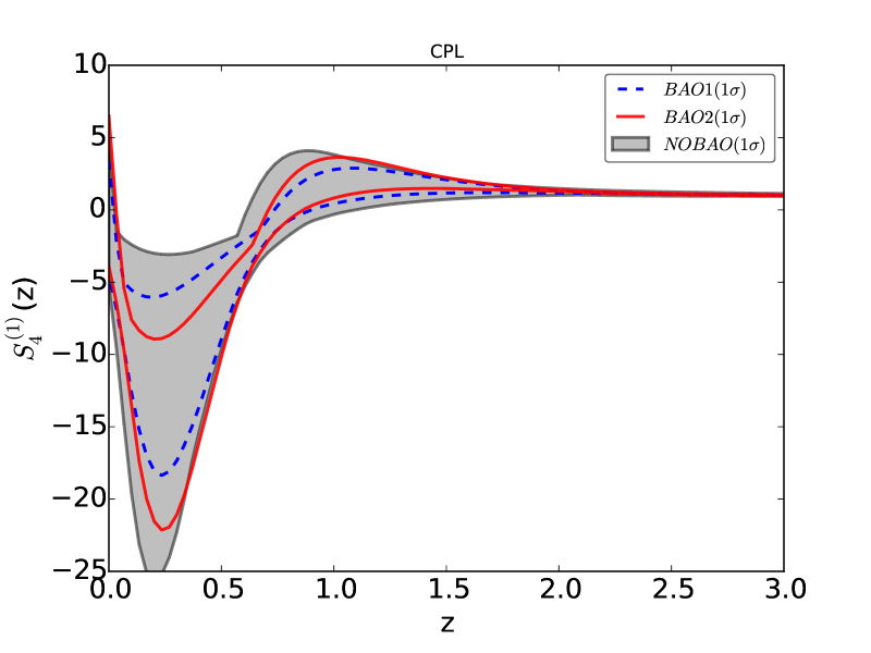
In Fig. 6, we plot the 1 confidence regions of statefinder hierarchy at redshift region [0,3] for the CDM model and the CPL model. Again, we see that the evolution trajectory of given by the CDM model is quite different from the results of the CPL model, which implies that the statefinder hierarchy is also a powerful tool that has the ability to distinguish different DE models. Moreover, we see that most of the 1 confidence regions of given by the two BAO data are overlap. This means that the effects of different BAO data can not be distinguishthed by using the statefinder either.
In addition, from Figs. 5 and 6 we see that for the CDM model, the 1 confidence regions of given by BAO1 and BAO2 seperate from the 1 regions given by NO BAO; in contrast, the 1 regions of given by BAO1 and BAO2 are enclosed by the 1 regions of NO BAO at . This means that compared with , is a better diagnosis tool (for similar results, see (Myrzakulov2013etc, )).
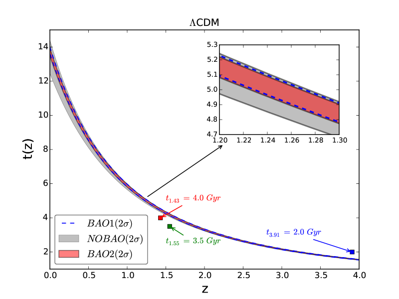
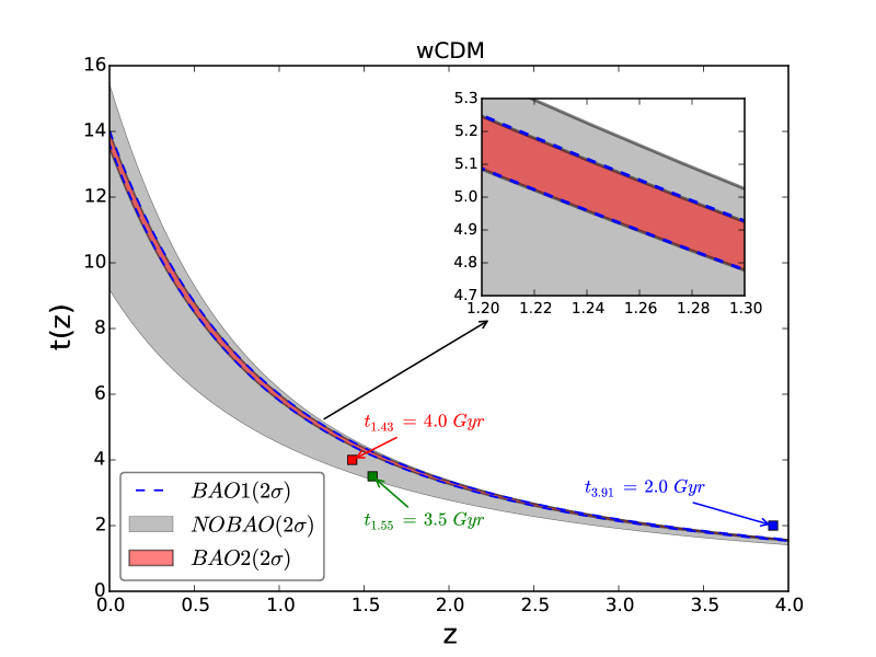
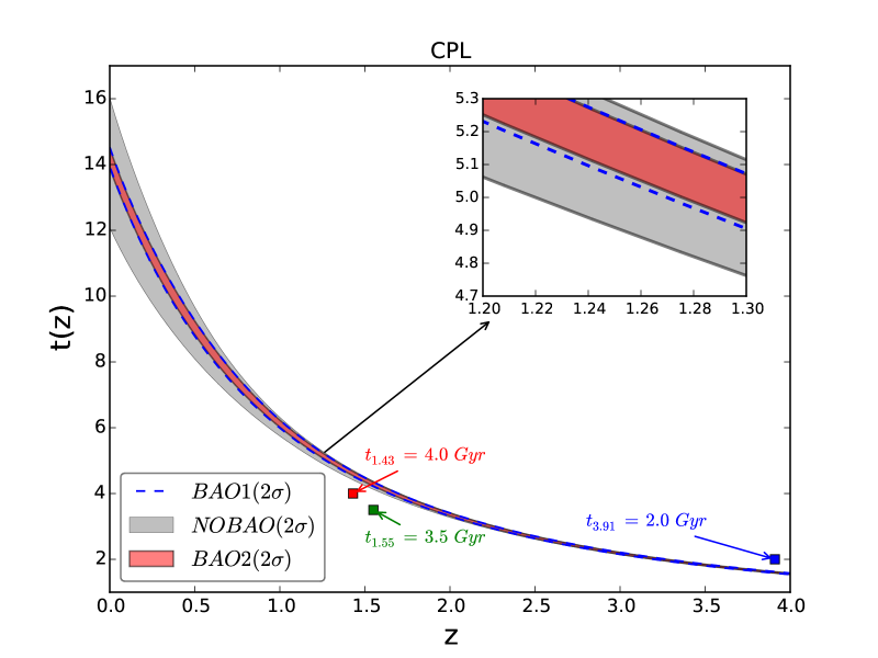
In Fig. 7, we plot the 2 confidence regions of cosmic age at redshift region [0,4] for the three DE models, where the three data points, , and , are also marked by Squares for comparison. We find that both and can be easily accommodated in all the three DE models, but the position of is significantly higher than the 2 upper bounds of all the three DE models. This means that the existence of the old quasar APM 08279+5255 can not be explained in the standard cosmology. This result is consistent with the conclusions of pervious studies Alcaniz03 . In addition, the 2 regions of given by BAO1 and BAO2 are almost overlap, showing that the impacts of different BAO data can not be distinguished by using the age data of OHRO.
IV Summary
In this work, we explore the cosmological implications of two types of BAO data. These two types BAO data are obtained by using the spherically averaged 1D galaxy clustering statistics (BAO1 data) and the anisotropic 2D galaxy clustering statistics (BAO2 data), respectively. So far as we know, the effects of different BAO data on cosmology-fits and corresponding cosmological consquences have not been studied in the past. So the main aim of our work is presenting a comprehensive and systematic investigation on the cosmological implications of different BAO data. To make a comparison, we also take into account the case without any BAO data.
Making use of the BAO1 and the BAO2 data, as well as the SNLS3 SNe Ia sample and the Planck distance priors data, we give the cosmological constraints of the CDM, the CDM and the CPL model. Then, according to the cosmological fitting results, we study the impacts of different BAO data on cosmological consquences, including parameter space, EoS, FoM, deceleration-acceleration transition redshift, Hubble parameter , deceleration parameter , statefinder hierarchy and , and cosmic age .
We find that: (1) For all the three DE models, NO BAO data always give a smallest fractional matter density , a largest fractional curvature density and a largest Hubble constant ; in contrast, BAO1 data always give a largest , a smallest and a smallest (see table 1). (2) For the CDM and the CPL model, NO BAO data always give a largest ; in contrast, BAO2 always give a smallest (see Figs. 1 and 2). (3) Compared with the case of BAO1, BAO2 data always give a slightly larger FoM, and thus can give a cosmological constraint with a slightly better accuracy (see table 2). (4) The impacts of different BAO data on the cosmic evolution and the comic age are very small, and can not be distinguished by using various dark energy diagnosis (see Figs. 3, 4, 5 and 6) and the cosmic age data (see Figs. 7).
It would be interesting to further explore the cosmological implications of these two types of BAO data by considering some other factors, such as interaction between dark sectors (Guo07, ; LiYH13, ), sterile neutrinos (Zhang2014a, ), and cosmic fate (Caldwell03, ). These issues will be studied in future works.
Acknowledgements.
SW is supported by the National Natural Science Foundation of China under Grant No. 11405024 and the Fundamental Research Funds for the Central Universities under Grant No. 16lgpy50. ML is supported by the National Natural Science Foundation of China (Grant No. 11275247, and Grant No. 11335012) and a 985 grant at Sun Yat-Sen University.References
- (1) A. G. Riess et al. AJ, 116, 1009 (1998); S. Perlmutter et al. ApJ, 517, 565 (1999).
- (2) R. R. Caldwell, and M. Kamionkowski, Ann. Rev. Nucl. Part. Sci., 59, 397 (2009); M. Li, X. D. Li, S. Wang, et al. Commun. Theor. Phys., 56, 525 (2011); K. Bamba, S. Capozziello, S. Nojiri, et al. Ap&SS, 342, 155 (2012); M. Li, X. D. Li, S. Wang, et al. Frontiers of Physics, 8, 828 (2013); D. H. Weinberg et al. Physics Reports, 530, 87 (2013); S. Wang, Y. Wang, and M. Li, arXiv:1612.00345.
- (3) C. Blake, and G. Glazebrook, ApJ, 594, 665 (2003); H. J. Seo, and D. J. Eisenstein, ApJ, 598, 720 (2003);
- (4) D. J. Eisenstein ApJ, 633, 560 (2005)
- (5) W. J. Percival et al. MNRAS, 401, 2148 (2010)
- (6) M. Tegmark, et al. Phys. Rev. D, 74, 123507 (2006); F. Beutler, et al. MNRAS, 416, 3017 (2011); C. Blake, et al. MNRAS, 415, 2892 (2011); C. Blake, et al. MNRAS, 418, 1707 (2011); X. Xu, N. Padmanabhan, D. J. Eisenstein, et al. MNRAS, 427, 2146 (2012)
- (7) N. Padmanabhan, et al. MNRAS, 427, 2132 (2012)
- (8) L. Anderson et al. MNRAS, 427, 3435 (2012)
- (9) . Aubourg et al. arXiv:1411.1074
- (10) A. N. bazajian et al. ApJS, 182, 543 (2009)
- (11) D. J. Eisenstein et al. AJ, 142, 72 (2011)
- (12) T. Okumura et al. ApJ, 676, 889 (2008); E. Gaztaaga, A. Cabre, L. Hui, MNRAS, 399, 1663 (2009); E. A. Kazin, A. G. Snchez, and M. R. Blanton, MNRAS, 419, 3223 (2012); X. Xu, A. J. Cuesta, N. Padmanabhan, et al. MNRAS, 431, 2834 (2013); L. Anderson et al. MNRAS, 439, 83 (2014); Y.-S. Song, T. Okumura, and A. Taruya, Phys. Rev. D, 89, 103541 (2014); E. V. Linder, M. Oh, T. Okumura, et al. Phys. Rev. D, 063525 (2014).
- (13) L. Anderson et al. MNRAS, 441, 24 (2014);
- (14) C. H. Chuang, and Y. Wang, MNRAS, 426, 226 (2012); C. H. Chuang, and Y. Wang, MNRAS, 431, 2634 (2013); C. H. Chuang, and Y. Wang, MNRAS, 435, 255 (2013).
- (15) M. D. P. Hemantha, Y. Wang, and C. -H. Chuang, MNRAS, 445, 3737 (2014)
- (16) C. Alcock, and B. Paczynski, 1979, Nature, 281, 358.
- (17) G. E. Addison, G. Hinshaw, and M. Halpern, MNRAS, 436 : 1674-1683 (2013); C. Cheng, and Q. G. Huang, Sci. China Phys. Mech. Astron., 58, 099801 (2015); P. X. Wu, Z. X. Li, and H. W. Yu, arXiv:1501.01818.
- (18) A. Conley et al. ApJS, 192, 1 (2011)
- (19) Y. Wang, and S. Wang, Phys. Rev. D, 88, 043522 (2013)
- (20) M. Chevallier, and D. Polarski, Int. J. Mod. Phys. D, 10, 213 (2001); E. V. Linder, Phys.Rev.Lett, 90, 091301 (2003).
- (21) D. Huterer, and G. Starkman, Phys. Rev. Lett., 90, 031301 (2003); D. Huterer, and A. Cooray, Phys. Rev. D 71, 023506 (2005).
- (22) Q.-G. Huang, M. Li, X.-D. Li, et al. Phys. Rev. D 80, 083515 (2009); S. Wang, X.-D. Li, and M. Li, Phys. Rev. D 83, 023010 (2011); X.-D. Li, S. Li, S. Wang, et al. JCAP 1107, 011 (2011).
- (23) A. Albrecht, G. Bernstein, R. Cahn, et al. arXiv:astro-ph/0609591
- (24) A. Albrecht, and G. Bernstein, Phys.Rev.D 75, 103003 (2007); S. Sullivan, A. Cooray, and D. Holz, JCAP, 0709, 004 (2007); D. Sarkar et al. Phys. Rev. Lett, 100, 241302 (2008); Y. Wang, Phys.Rev.D, 77, 123525 (2008).
- (25) M. Arabsalmani, and V. Sahni, Phys.Rev.D, 83, 04350 (2011)
- Alcaniz and Lima (1999) J. S. Alcaniz and J. A. S. Lima, Astrophys. J. 521, L87 (1999); S. Wang, Y. Zhang, and T.-Y. Xia, JCAP 0810, 037 2008; M.-X. Lan, M. Li, X.-D. Li, et al. Phys. Rev. D 82, 023516 (2010); C.A.P. Bengaly Jr., M.A. Dantas, J.C. Carvalho, et al. Astron. Astrophys. 561, A44 (2014); S. Liu and T. J. Zhang, Phys. Lett. B 733, 69 (2014)
- (27) S. Wang, and Y. Wang, Phys. Rev. D, 88, 043511 (2013)
- (28) W. S. Zhang, C. Cheng, Q.-G. Huang, et al. Sci China-Phys Mech Astron, 55, 2244 (2012); L. J. Zhou, and S. Wang, Sci. China-Phys. Mech. Astron. 59, 670411 (2016); S. Wang, S. X. Wen, L. J. Zhou, et al. arXiv:1605.04356.
- (29) D. J. Eisenstein, and W. Hu, ApJ, 496, 605 (1998).
- (30) Y. Wang, MNRAS, 443, 2950 (2014).
- (31) G. M. Mohlabeng, and J. P. Ralston, MNRAS, 439, L16 (2013).
- (32) D. Scolnic et al. ApJ, 795, 45 (2014).
- (33) H. Shariff, X. Jiao, R. Trotta, D. A. van. Dyk, ApJ, 827, 1 (2016); M. Li, N. Li, S. Wang, et al. MNRAS, 460, 2586 (2016).
- (34) S. Wang, Y. H. Li, and X. Zhang, Phys. Rev. D, 89, 063524 (2014); S. Wang, Y. Z. Wang, J. J. Geng, et al. Eur. Phys. J. C 74: 3148 (2014); S. Wang, Y. Z. Wang, and X. Zhang, Commun. Theor. Phys. 62, 927 (2014); S. Wang, J. J. Geng, Y. L. Hu, et al. Sci. China Phys. Mech. Astron. 58: 019801 (2015); S. Wang, S. Wen, and M. Li, arXiv:1606.01779.
- (35) J. Marriner et al. ApJ, 740, 72 (2011)
- (36) G. R. Bengochea, Phys. Lett. B 696, 5 (2011); G. R. Bengochea, and M. E. De Rossi, Phys. Lett. B 733, 258 (2014)
- (37) Y. Hu, M. Li, N. Li, et al. Astron. Astrophys., 592, A101 (2016)
- (38) Y. Wang, and P. Mukherjee, Phys.Rev.D, 76, 103533 (2007)
- (39) W. Hu, and N. Sugiyama, ApJ, 471: 542-470 (1996)
- (40) H. Li, J. Q. Xia, G. B. Zhao, et al. ApJ 683, L1 (2008)
- (41) Y. H. Li, S. Wang, X. D. Li, et al. JCAP, 1302, 033 (2013)
- (42) A. Lewis, and S. Bridle, Phys. Rev. D, 66, 103511 (2002)
- (43) L. Samushia et al. MNRAS, 429, 1514 (2013)
- (44) T. Delubac et al. A&A, 574, A59 (2015)
- (45) J. A. S. Lima, J. F. Jesus, R. C. Santos, et al. arXiv: 1205.4688
- Dunlop et al. (1996) J. Dunlop, et al., Nature 381, 581 (1996)
- Dunlop (1999) J. Dunlop, The Most Distant Radio Galaxies, Kluwer, Dordrecht (1999)
- Hasinger, Schartel, & Komossa (2002) G. Hasinger, N. Schartel, and S. Komossa, Astrophys. J. 573, L77 (2002)
- (49) J. S. Alcaniz, J. A. S. Lima, J. V. Cunha, MNRAS 340 L39 (2003); H. Wei, and Zhang, S. N., Phys. Rev. D 76, 063003 (2007); S. Wang, and Y. Zhang, Phys. Lett. B 669, 201 (2008); S. Wang, X. D. Li, and M. Li, Phys. Rev. D, 82, 103006 (2010); J. Cui, and X. Zhang, Phys. Lett. B 690, 233 (2010); X. P. Yan, D. Z. Liu, and H. Wei, Phys. Lett. B 742, 149 (2015)
- (50) A. G. Snchez et al. MNRAS, 440, 2692 (2014); L. Samushia et al. MNRAS, 439, 3504 (2014); E. A. Kazin et al. MNRAS, 441, 3524 (2014)
- (51) P. A. R. Ade et al. arXiv:1502.01589
- (52) C. Clarkson, M. Cortes, B. A. Bassett, JCAP, 0708, 011 (2007)
- (53) X. Ding, M. Biesiada, S. Cao, Z. Li, Z.H. Zhu, Astrophys. J. 803, L22 (2015); R. Y. Guo and X. Zhang, Eur. Phys. J. C 76, 163 (2016).
- (54) V. Sahni, A. Shafieloo, and A. A. Starobinsky, ApJ, 793, L40 (2014).
- (55) A. Shafieloo, V. Sahni, and A. A. Starobinsky, Phys. Rev. D, 80, 101301(R) (2009).
- (56) S. Wang, Y. Hu, M. Li, et al. ApJ 821, 60 (2016).
- (57) M. S. Turner, and A. G. Riess, AJ, 569, 18 (2002); J. V. Cunha, and J. A. S. Lima, MNRAS, 390, 210 (2008); O. Farooq, and B. Ratra, ApJ, 766, L7 (2013).
- (58) R. Myrzakulov, and M. Shahalam, JCAP, 1310, 047 (2013); J. Li, R. Yang, and B. Chen, JCAP, 1412, 043 (2014); J. L. Cui, and J. F. Zhang, Eur. Phys. J. C, 74, 2849 (2014).
- (59) Z.-K. Guo, N. Ohta, and S. Tsujikawa, Phys. Rev. D, 76, 023508 (2007); M. Li, X. D. Li, S. Wang, et al. JCAP, 0912, 014 (2009); M. Li, X. D. Li, S. Wang, et al. JCAP, 0906, 036 (2009); J. H. He, B. Wang, E. Abdalla, D. Pavon, JCAP, 1012, 022 (2010); Y. H. Li, J. F. Zhang, and X. Zhang, Phys. Rev. D 90, 063005 (2014); Y. H. Li, J. F. Zhang, and X. Zhang, Phys. Rev. D 90, 123007 (2014).
- (60) J. F. Zhang, J. J. Geng, and X. Zhang, JCAP, 1410, 044 (2014); J. F. Zhang, Y. H. Li, and X. Zhang, Eur. Phys. J. C, 74, 2954 (2014); J. F. Zhang, Y. H. Li, and X. Zhang, Phys. Lett. B, 740, 359 (2015).
- (61) R. R. Caldwell, M. Kamionkowski, N. N. Weinberg, Phys. Rev. Lett, 91, 071301 (2003); X. D. Li, S. Wang, Q. G. Huang, et al. Sci. China Phys. Mech. Astron., 55, 1330 (2012); Z. Zhang, M. Li, X. D. Li, et al. Mod. Phys. Lett. A, 27, 1250115 (2012).