On the approximation of the principal eigenvalue for a class of nonlinear elliptic operators

Abstract

We present a finite difference method to compute the principal eigenvalue and the corresponding eigenfunction for a large class of second order elliptic operators including notably linear operators in nondivergence form and fully nonlinear operators.
The principal eigenvalue is computed by solving a finite-dimensional nonlinear min-max optimization problem. We prove the convergence of the method and we discuss its implementation. Some examples where the exact solution is explicitly known show the effectiveness of the method.

MSC 2000:

35J60, 35P30, 65M06.

Keywords:

Principal eigenvalue, nonlinear elliptic operators, finite difference schemes, convergence.

1 Introduction

Consider the elliptic self-adjoint operator

$$Lu(x)={\partial}_{i}\left(a_{ij}(x){\partial}_{j}u(x)\right),$$ (1.1)

where $a_{ij}=a_{ji}$ are smooth functions in $\Omega$, a smooth bounded open subset of ${\mathbb{R}}^{n}$, satisfying $a_{ij}\xi_{i}\xi_{j}\geq\alpha|\xi|^{2}$ for some $\alpha>0$. It is well-known that the minimum value $\lambda_{1}$ in the Rayleigh-Ritz variational formula

$$\lambda_{1}=\inf_{\varphi\in H^{1}_{0}(\Omega),\varphi\not\equiv 0}\frac{-\int_{\Omega}\varphi(x)\,L\varphi(x)\,\,dx\,}{\|\varphi\|^{2}_{L^{2}(\Omega)}}=\inf_{\varphi\in H^{1}_{0}(\Omega),\varphi\not\equiv 0}\frac{\int_{\Omega}a_{ij}(x){\partial}_{j}\varphi(x){\partial}_{i}\varphi(x)\,\,dx\,}{\|\varphi\|^{2}_{L^{2}(\Omega)}}$$

is attained at some function $w_{1}$ satisfying

$$\left\{\begin{array}[]{ll}Lw_{1}(x)+\lambda_{1}w_{1}(x)=0&x\in\Omega,\\ w_{1}(x)=0&x\in\partial\Omega.\end{array}\right.$$

The number $\lambda_{1}$ is usually referred to as the principal eigenvalue of $L$ in $\Omega$ and $w_{1}$ is the corresponding principal eigenfunction. For operators of the form (1.1) and also more general linear operator in divergence form there is a vast literature on computational methods for the principal eigenvalue, see for example [2], [10], [14], [22].

General non-divergence type elliptic operators, namely

$$Lu(x)=a_{ij}(x){\partial}_{ij}u(x)+b_{i}(x){\partial}_{i}u(x)+c(x)u$$ (1.2)

are not self-adjoint and the spectral theory is then much more involved: in particular, the Rayleigh-Ritz variational formula is not available anymore. In the seminal paper [12] by M.D. Donsker and S.R.S. Varadhan, a min-max formula for the principal eigenvalue of a class of elliptic operators $L$ including (1.2) was proved, namely

$$\lambda_{1}=-\inf_{\varphi\in C^{2}(\Omega),\varphi>0}\;\sup_{x\in\Omega}\frac{L\varphi(x)}{\varphi(x)}.$$ (1.3)

In that papers other representation formulas for $\lambda_{1}$ were also proposed in terms of large deviations and of the average long run time behavior of the positive semigroup generated by $L$. A further crucial step in that direction is the paper [6] by H. Berestycki, L. Nirenberg and S.R.S. Varadhan, where the validity of formula (1.3) is proved under mild smoothness assumptions ($\Omega$ a bounded open set and $a_{ij}\in C^{0}(\Omega)$, $b_{i}$, $c\in L^{\infty}(\Omega)$). Moreover it is proved that (1.3) is equivalent to

$$\lambda_{1}:=\sup\{\lambda\in{\mathbb{R}}:\,\exists\,\varphi>0\;\text{ such that}\;L\varphi+\lambda\varphi\leq 0\quad\text{in $\Omega$}\}.\,$$

Following this path of ideas, notions of principal eigenvalue for fully nonlinear uniformly elliptic operators of the form

$$F[u]=F(x,u(x),Du(x),D^{2}u(x))$$

have been introduced and analyzed in [1], [5], [8], [11], [15], [20]. A by now established definition of principal eigenvalue is given by

$$\lambda_{1}:=\sup\{\lambda\in{\mathbb{R}}:\,\exists\,\varphi>0\;\text{ such that}\;F[\varphi]+\lambda\varphi\leq 0\quad\text{in $\Omega$}\}\,$$ (1.4)

where the inequality in (1.4) is intended in viscosity sense. It is possible to prove under appropriate assumptions, see (2.1)-(2.2), that there exists a viscosity solution $w_{1}$ of

$$\left\{\begin{array}[]{ll}F[w_{1}]+\lambda_{1}w_{1}(x)=0&x\in\Omega,\\ w_{1}(x)=0&x\in\partial\Omega.\end{array}\right.$$ (1.5)

Moreover the characterization (1.3) still holds in this nonlinear setting.

As it is well-known, the principal eigenvalue plays a key role in several respects, both in the existence theory and in the qualitative analysis of elliptic partial differential equations as well in applications to large deviations [1], [12], bifurcation issues [20], ergodic and long run average cost problems in stochastic control [4]. For linear non self-adjoint operators and, a fortiori, for nonlinear ones the principal eigenvalue can be explicitly computed only in very special cases, see e.g. [9, 21], hence the importance to devise numerical algorithms for the problem. But, apart some specific case (see [7] for the $p$-Laplace operator), approximation schemes and computational methods are not available in the literature, at least at our present knowledge.

The aim of this paper is to define a numerical scheme for the principal eigenvalue of nonlinear uniformly elliptic operators via a finite difference approximation of formula (1.3). More precisely, denoting by ${\mathbb{Z}}^{n}_{h}=h{\mathbb{Z}}^{n}$ the orthogonal lattice in ${\mathbb{R}}^{n}$ where $h>0$ is a discretization parameter, we consider a discrete operator $F_{h}$ acting on functions defined on a discrete subset $\Omega_{h}\subset{\mathbb{Z}}^{n}_{h}$ of $\Omega$ and the corresponding approximated version of (1.3), namely

$$\lambda_{1,h}=-\inf_{\varphi>0}\sup_{x\in\Omega_{h}}\frac{F_{h}[\varphi](x)}{\varphi(x)}.$$ (1.6)

As for the approximating operators $F_{h}$, we consider a specific class of finite difference schemes introduced in [17], [18] since they satisfy some useful properties for the convergence analysis.

We prove that if $F$ is uniformly elliptic and satisfies in addition some quite natural further conditions, then it is possible to define a finite difference scheme $F_{h}$ such that the discrete principal eigenvalues $\lambda_{1,h}$ and the associated discrete eigenfunctions $w_{1,h}$ converge uniformly in $\Omega$, as the mesh step $h$ is sent to $0$, respectively to the principal eigenvalue $\lambda_{1}$ and to the corresponding eigenfunction $w_{1}$ for the original problem (1.5). It is worth pointing out that the proof of our main convergence result, Theorem 3.2, cannot rely on standard stability results for fully nonlinear partial differential equations, see [3], since the limit problem does not satisfy a comparison principle (see Remark 3.1 for details).

We mention that our approach is partially inspired by the paper [13] where a similar approximation scheme is proposed for the computation of effective Hamiltonians occurring in the homogenization of Hamilton-Jacobi equations which can be characterized by a formula somewhat similar to (1.3).

In Section 2 we introduce the main assumptions and we investigate some issues related to the Maximum Principle for discrete operators. In Section 3 we study the approximation method for a class of finite difference schemes and we prove the convergence of the scheme. In Section 4 we show that under some additional structural assumptions on $F_{h}$ the inf-sup problem (1.6) can be transformed into a convex optimization problem on the nodes of the grid and we discuss its implementation. A few tests which show the efficiency of our method on some simple examples are reported in Section 4 as well.

2 The Maximum Principle for discrete operators

We start by fixing some notations and the assumptions on the operator $F$. Set $\Gamma=\Omega\times{\mathbb{R}}\times{\mathbb{R}}^{n}\times S^{n}$ , where $S^{n}$ denotes the linear space of real, symmetric $n\times n$ matrices. The function $F(x,z,p,r)$ is assumed to be continuous on $\Gamma$ and locally uniformly Lipschitz continuous with respect to $z,p,r$ for each fixed $x\in\Omega$. We will also suppose that the partial derivatives $F_{r}$, $F_{p}$, $F_{z}$ satisfy the following structure conditions:

$$0<aI\leq F_{r}\leq AI,\quad|F_{p}|\leq\mu_{1},\quad-\mu_{0}\leq F_{z}\leq 0.$$ (2.1)

for some constants $a$, $A$, $\mu_{0}$, $\mu_{1}$. A further condition is the positive homogeneity of degree $1$, that is

$$F(x,tz,tp,tr)=tF(x,z,p,r)\qquad\forall t\geq 0.$$ (2.2)

The principal eigenvalue of problem (1.5) is defined by

$$\lambda_{1}=\sup\{\lambda:\,\exists\,\varphi>0\;{\rm such\,that}\;F[\varphi]+\lambda\varphi\leq 0\ \mbox{in}\ \Omega\},$$

where the differential inequality $F[\varphi]+\lambda\varphi\leq 0$ is meant in the viscosity sense. Under assumptions (2.1)-(2.2), there exists a viscosity solution of (1.5) and the characterization (1.3) of $\lambda_{1}$ holds (see [8], [11]).

Remark 2.1

It is possible to define

$$\lambda_{1}^{-}=\sup\{\lambda:\,\exists\,\varphi<0\;{\rm such\,that}\;F[\varphi]+\lambda\varphi\geq 0\ \mbox{in}\ \Omega\}.$$

When $F$ is not odd in its dependence on the Hessian, then in general $\lambda_{1}\neq\lambda_{1}^{-}$. Of course it is possible to see $\lambda_{1}^{-}$ as $\lambda_{1}$ of some other operator. Hence we will only consider in this paper $\lambda_{1}$. For example, for the extremal Pucci operators ${\mathcal{M}}^{+}_{a,A}(D^{2}u):=\sup_{aI\leq B\leq AI}tr(AD^{2}u)$ and ${\mathcal{M}}^{-}_{a,A}(D^{2}u):=\inf_{aI\leq B\leq AI}tr(AD^{2}u)$, since ${\mathcal{M}}^{+}_{a,A}(-M)=-{\mathcal{M}}^{-}_{a,A}(M)$, the following holds

$$\lambda_{1}^{-}({\mathcal{M}}^{+}_{a,A})=\lambda_{1}({\mathcal{M}}^{-}_{a,A}).$$

Remark 2.2

The assumption $F_{z}\leq 0$, i.e. the monotonicity of the differential operator in the zero-order term, could be removed. Indeed $\bar{F}:=F-c_{0}z$, with $c_{0}$ large, satisfies this assumption, moreover $\bar{F}$ and $F$ have the same principal eigenfunction and the eigenvalues differ by $c_{0}$.

We now describe the discrete setting that we shall consider. Given $h>0$, let ${\mathbb{Z}}^{n}_{h}=h{\mathbb{Z}}^{n}$ denote the orthogonal lattice in ${\mathbb{R}}^{n}$. Let $F_{h}$ be a discrete operator acting on functions defined in $\Omega_{h}\subset{\mathbb{Z}}^{n}_{h}$. We shall consider an approximation of (1.5) (which can be seen also as an eigenvalue problem for the discrete operator $F_{h}$). We look for a number $\lambda$ and a positive function $w$ such that

$$\left\{\begin{array}[]{ll}F_{h}(x,w(x),[w]_{x})+\lambda w(x)=0&x\in\Omega_{h},\\ w(x)=0&x\in\partial\Omega_{h},\end{array}\right.$$ (2.3)

where

• $h>0$ is the discretization parameter ($h$ is meant to tend to $0$),

• $x\in\Omega_{h}$ is the point where (1.5) is approximated,

• $w$ is a real valued mesh function in ${\mathbb{Z}}^{n}_{h}$ meant to approximate the viscosity solution of (1.5),

• $[\cdot]_{x}$ represents the stencil of the scheme, i.e. the points in $\Omega_{h}\backslash\{x\}$ where the value of $u$ is computed for writing the scheme at the point $x$ (we assume that $[w]_{x}$ is independent of $w(y)$ for $|x-y|>Mh$ for some fixed $M\in{\mathbb{N}}$).

We denote by ${\cal C}_{h}$ the space of the mesh functions defined on $\overline{\Omega}_{h}$ and we introduce some basic assumptions for the scheme $F_{h}$ (see [17], [18]).

• The operator $F_{h}$ is of positive type, i.e. for all $x\in\Omega_{h}$, $z,\tau\in{\mathbb{R}}$, $u,\eta\in{\cal C}_{h}$ satisfying $0\leq\eta(y)\leq\tau$ for each $y\in\Omega_{h}$, then

  $$F_{h}(x,z,[u+\eta]_{x})\geq F_{h}(x,z,[u]_{x})\geq F_{h}(x,z+\tau,[u+\eta]_{x})$$

• The operator $F_{h}$ is positively homogeneous, i.e. for all $x\in\Omega_{h}$, $z\in{\mathbb{R}}$, $u\in{\cal C}_{h}$ and $t\geq 0$, then

  $$F_{h}(x,tz,[tu]_{x})=tF_{h}(x,z,[u]_{x}).$$

• The family of operators $\{F_{h},0<h\leq h_{0}\}$, where $h_{0}$ is a positive constant, is consistent with the operator $F$ on the domain $\Omega\subset{\mathbb{R}}^{n}$, i.e. for each $u\in C^{2}(\Omega)$

  $$\sup_{\Omega_{h}}\left|F(x,u(x),Du(x),D^{2}u(x))-F_{h}(x,u(x),[u]_{x})\right|\to 0\quad\text{as $h\to 0$,}$$

  uniformly on compact subset of $\Omega$.

We study below some properties related to the maximum principle and a comparison result for the operator $F_{h}$. Let us start by the following definitions:

Definition 2.1

A function $u\in{\cal C}_{h}$ is a subsolution (respectively $v\in{\cal C}_{h}$ is a supersolution) of

$$F_{h}(x,u(x),[u]_{x})=f(x)\qquad x\in\Omega_{h}$$ (2.4)

if

$$F_{h}(x,u(x),[u]_{x})\geq f(x),\qquad x\in\Omega_{h}$$

$$\left(\text{respectively, }F_{h}(x,v(x),[v]_{x})\leq f(x),\qquad x\in\Omega_{h}\right).$$

Definition 2.2

The Maximum Principle holds for the operator $F_{h}$ in $\Omega_{h}$ if

$$\left\{\begin{array}[]{ll}F_{h}(x,u(x),[u]_{x})\geq 0&\text{in $\Omega_{h}$,}\\ u\leq 0&\text{on $\partial\Omega_{h}$,}\end{array}\right.$$ (2.5)

implies $u\leq 0$ in $\Omega_{h}$.

Proposition 2.1

Assume that $F_{h}$ is of positive type and positive homogeneous and satisfies either

$$\begin{split}\text{for all $z\in{\mathbb{R}}$, $u,\eta\in{\cal C}_{h}$ satisfying $0\leq\eta(y)$ and $max_{y\in[\cdot]_{x}}\eta(y)>0$,}\\ \text{then }\quad F_{h}(x,z,[u+\eta]_{x})>F_{h}(x,z,[u]_{x})\qquad\end{split}$$ (2.6)

or

$$\begin{split}\text{for all $z,\tau\in{\mathbb{R}}$, $u,\eta\in{\cal C}_{h}$ satisfying $0\leq\eta(y)\leq\tau$ for each $y$, then}\\ F_{h}(x,z,[u]_{x})\geq F_{h}(x,z+\tau,[u+\eta]_{x})+c_{0}\tau\qquad\end{split}$$ (2.7)

for some positive constants $c_{0}$. Then the Maximum Principle holds for the operator $F_{h}$ in $\Omega_{h}$ .

Proof  Assume by contradiction that $u$ satisfies (2.5) and $M:=\max_{\overline{\Omega}_{h}}u>0$. Let $\bar{x}\in\Omega_{h}$ be such that $u(\bar{x})=M$. Since $u\leq 0$ on $\partial\Omega_{h}$, it is not restrictive to assume that there exists $y\in\Omega_{h}$ such that $u(y)<u(\bar{x})=M$. Hence

$$0 \leq F_{h}(\bar{x},u(\bar{x}),[u]_{\bar{x}})\leq F_{h}(\bar{x},u(\bar{x})-M,[u-M]_{\bar{x}})$$

$$<F_{h}(\bar{x},0,[0]_{\bar{x}})=0,$$

a contradiction. A similar proof can be done with the assumption (2.7).

$\Box$

Remark 2.3

The assumptions (2.6) and (2.7) correspond to the uniform ellipticity and, respectively, to the strict monotonicity of the operator $F$ with respect to the zero-order term.

The following proposition shows that, as it is known in the continuous case (see for example [6, 8]), the validity of the Maximum Principle for subsolutions of the operator $F_{h}$ is equivalent to the positivity of the principal eigenvalue for $F_{h}$.

Proposition 2.2

Assume that the scheme $F_{h}$ is of positive type and that it is positively homogeneous. Suppose that for $\lambda\in{\mathbb{R}}$, there exists a nonnegative grid function $\varphi$ with $\varphi>0$ in $\Omega_{h}$ such that $F_{h}[\varphi]+\lambda\varphi\leq 0$. If, for $\tau<\lambda$, the function $u$ satisfies

$$\left\{\begin{array}[]{ll}F_{h}(x,u(x),[u]_{x})+\tau u\geq 0&\text{in $\Omega_{h}$}\\ u\leq 0&\text{on $\partial\Omega_{h}$,}\end{array}\right.$$

then $u\leq 0$ in $\Omega_{h}$, i.e. $F_{h,\tau}[\cdot]=F_{h}[\cdot]+\tau\cdot$ satisfies the Maximum Principle.

Proof  Suppose by contradiction that $\max_{\overline{\Omega}_{h}}\{u\}>0$. Let $\varphi$ as in the statement and set $L({\gamma})=\max_{\Omega_{h}}\{u-{\gamma}\varphi\}$ (note that the maximum is taken only with respect to the internal points). Then $L:[0,\infty)\to{\mathbb{R}}$ is continuous, decreasing, $L(0)>0$ and $L({\gamma})\to-\infty$ for ${\gamma}\to+\infty$. Hence there exists ${\gamma}^{\prime}>0$ such that $L({\gamma}^{\prime})=0$. Moreover, since $u-{\gamma}^{\prime}\varphi\leq 0$ on $\partial\Omega$, we also have $\max_{\overline{\Omega}_{h}}\{u-{\gamma}^{\prime}\varphi\}=0$. Let $0<{\gamma}<{\gamma}^{\prime}$ be such that

$$\frac{{\gamma}}{{\gamma}^{\prime}}\lambda>\tau$$ (2.8)

and set $\psi={\gamma}\varphi$. Then $F_{h}[\psi]+\lambda\psi\leq 0$ and $M=\max_{\overline{\Omega}_{h}}\{u-\psi\}=(u-\psi)(\bar{x})>0$ for some $\bar{x}\in\Omega_{h}$. Hence $\psi(\bar{x})+M=u(\bar{x})$ and $\psi(x)+M\geq u(x)$. Since $F_{h}$ is of positive type, it follows that

$$F_{h}(x,\psi(\bar{x}),[\psi]_{\bar{x}}) \geq F_{h}((x,\psi(\bar{x})+M,[\psi+M]_{\bar{x}})=F_{h}(x,u(\bar{x}),[\psi+M]_{\bar{x}})$$

$$\geq F_{h}(x,u(\bar{x}),[u]_{\bar{x}}).$$

Then

$$\tau u(\bar{x})\geq-F_{h}[u](\bar{x})\geq-F_{h}[\psi](\bar{x})\geq\lambda\psi(\bar{x})=\lambda{\gamma}\varphi(\bar{x})\geq\lambda\frac{{\gamma}}{{\gamma}^{\prime}}u(\bar{x})$$

and therefore a contradiction to (2.8). $\Box$

The following result gives a comparison principle for (2.4).

Proposition 2.3

Assume that $F_{h}$ is of positive type and it satisfies either (2.6) or (2.7). Let $u$ and $v$ be a subsolution and respectively a supersolution of (2.4) such that $u\leq v$ on ${\partial}\Omega_{h}$. Then $u\leq v$ in $\overline{\Omega}_{h}$.

Proof  Suppose by contradiction that $M:=\max_{\overline{\Omega}_{h}}\{u-v\}>0$ and let $\bar{x}\in\Omega_{h}$ be such that $u(\bar{x})-v(\bar{x})=M$. Hence $v+M\geq u$ in $\Omega_{h}$ and it is not restrictive to assume that $\max_{y_{\in}[\cdot]_{\bar{x}}}(v+M-u)>0$. It follows that

$$f(\bar{x})\leq F_{h}(\bar{x},u(\bar{x}),[u]_{\bar{x}}) =F_{h}(\bar{x},v(\bar{x})+M,[u]_{\bar{x}})<F_{h}(\bar{x},v(\bar{x})+M,[v+M]_{\bar{x}})$$

$$\leq F_{h}(\bar{x},v(\bar{x}),[v]_{\bar{x}})\leq f(\bar{x})$$

and therefore a contradiction. A similar proof can be carried on under assumption (2.7). $\Box$

3 Approximation of the principal eigenvalue

In this section we consider a specific class of finite difference schemes introduced in [18]. These schemes satisfy certain pointwise estimates which are the discrete analogues of those valid for a general class of fully nonlinear, uniformly elliptic equations.
We assume that for all $x\in{\mathbb{Z}}^{n}_{h}$, the stencil $[\cdot]_{x}$ of the scheme is given by $x+hY$ where $Y=\{y_{1},\dots,y_{k}\}\subset{\mathbb{Z}}^{n}$ is a finite set containing all the vectors of the canonical basis of ${\mathbb{R}}^{n}$. Then we consider a discrete operator $F_{h}$ in (2.3) given by a finite difference scheme written in the form

$$F_{h}[u]={{\cal F}}(x,u,{\delta}_{h}u,{\delta}^{2}_{h}u),$$ (3.1)

where ${\cal F}:{\mathbb{R}}^{n}\times{\mathbb{R}}\times{\mathbb{R}}^{Y}\times{\mathbb{R}}^{Y}\to{\mathbb{R}}$ and for $y\in Y$, $u\in{\cal C}_{h}$

$$\delta_{h,y}^{\pm}u(x) =\pm\frac{u(x\pm hy)-u(x)}{h|y|},$$

$$\delta_{h,y}u(x) =\frac{1}{2}\{\delta_{h,y}^{+}u(x)+\delta_{h,y}^{-}u(x)\}=\frac{u(x+hy)-u(x-hy)}{2h|y|},$$

$$\delta^{2}_{h,y}u(x) =\delta_{h,y}^{+}\delta_{h,y}^{-}u(x)=\frac{u(x+hy)+u(x-hy)-2u(x)}{h^{2}|y|^{2}},$$

$${\delta}_{h}u =\{{\delta}_{h,y}u:\,y\in Y\},\quad{\delta}^{2}_{h}u=\{{\delta}^{2}_{h,y}u:\,y\in Y\}.$$

Set $\tilde{\Gamma}:={\mathbb{R}}^{n}\times{\mathbb{R}}\times{\mathbb{R}}^{Y}\times{\mathbb{R}}^{Y}$ and denote by $(x,z,q,s)$ the generic points in $\tilde{\Gamma}$. The operator $F_{h}$ given by (3.1) is of positive type if

$$\frac{\partial{\cal F}}{\partial s_{y}}-\frac{|hy|}{2}\left|\frac{\partial{\cal F}}{\partial q_{y}}\right|\geq 0\quad\forall y\in Y,$$ (3.2)

$$\frac{\partial{\cal F}}{\partial z}\leq 0,$$ (3.3)

and positively homogeneous if

$${\cal F}(x,tz,tq,ts)=t{\cal F}(x,z,q,s)\qquad\forall t\geq 0.$$

Moreover if $F$ in (1.5) satisfies the assumptions (2.1), then it is always possible to find a scheme of type (3.1) which is consistent with $F$ and which, besides (3.2)-(3.3), satisfies for all $y\in Y$, the bounds

$$\frac{\partial{\cal F}}{\partial s_{y}}-\frac{|hy|}{2}\left|\frac{\partial{\cal F}}{\partial q_{y}}\right|\geq{\alpha}_{0},\qquad\frac{\partial{\cal F}}{\partial s_{y}}\leq a_{0},\qquad\left|\frac{\partial{\cal F}}{\partial q_{y}}\right|\leq b_{0}$$ (3.4)

where ${\alpha}_{0}$, $a_{0}$, $b_{0}$ are constants depending on $a$, $A$, $\mu_{0}$, $\mu_{1}$ in (2.1) (see [17], [18]). Note that in particular (3.4) implies (2.6).
We recall some important properties of the previous scheme (for the proof we refer to [18])

Proposition 3.1

Assume (3.2)-(3.4) and let $f$, $g$ be two given mesh functions. Then for every $h>0$ sufficiently small there exists a unique solution $u_{h}:\Omega_{h}\to{\mathbb{R}}$ to the Dirichlet problem

$$\left\{\begin{array}[]{ll}F_{h}(x,u(x),[u]_{x})=f&x\in\Omega_{h},\\ u=g&x\in{\partial}\Omega_{h}.\end{array}\right.$$ (3.5)

Proposition 3.2

Assume (3.2)-(3.4) and let $u_{h}$ be a subsolution of (3.5). Then

$$\max_{\Omega_{h}}u_{h}\leq\max_{{\partial}\Omega_{h}}g+\frac{C}{{\alpha}_{0}}\left\{\sum_{x\in\Omega_{h}}h^{n}|f(x)|^{n}\right\}^{\frac{1}{n}},$$ (3.6)

where the constant $C$ is independent of $h$. Moreover if $u_{h}$ is a solution of (3.5), then for any $x,y\in\Omega_{h}$

$$|u_{h}(x)-u_{h}(y)|\leq C\frac{|x-y|^{\delta}}{R}\left(\max_{B_{R}^{h}}u_{h}+\frac{R}{{\alpha}_{0}}\left\{\sum_{x\in\Omega_{h}}h^{n}|f(x)|^{n}\right\}^{\frac{1}{n}}\right),$$ (3.7)

where $R=\min\{\mathrm{dist}(x,{\partial}\Omega_{h}),\mathrm{dist}(x,{\partial}\Omega_{h})\}$, $B_{R}^{h}=B(0,R)\cap\Omega_{h}$, ${\delta}$ and $C$ are positive constants independent of $h$.

We give an example of a scheme of the form (3.1). Consider the Hamilton-Jacobi-Bellman operator

$$F(x,u,Du(x),D^{2}u(x))=\sup_{{\alpha}\in A}\inf_{{\beta}\in B}L^{{\alpha}{\beta}}u(x)$$

where

$$L^{{\alpha}{\beta}}u(x)=a_{ij}^{{\alpha}{\beta}}(x)D_{ij}u+b_{i}^{{\alpha}{\beta}}(x)D_{i}u(x)+c^{{\alpha}{\beta}}(x)u(x).$$ (3.8)

It is always possible to rewrite the operator $L^{{\alpha}{\beta}}$ in (3.8) in the following form (see [18])

$$\overline{L}^{{\alpha}{\beta}}u(x)=\bar{a}_{k}^{{\alpha}{\beta}}(x)D^{2}_{y_{k}}u+\bar{b}_{k}^{{\alpha}{\beta}}(x)D_{y_{k}}u(x)+\bar{c}^{{\alpha}{\beta}}(x)u(x)$$

where $D_{y_{k}}u=\langle Du,y_{k}\rangle$ and $Y=\{y_{1},\dots,y_{k}\}\subset{\mathbb{Z}}^{n}$ is a finite set containing all the vectors of the canonical basis in ${\mathbb{R}}^{n}$. Moreover the coefficients $\bar{a}_{k}^{{\alpha}{\beta}}$, $\bar{b}_{k}^{{\alpha}{\beta}}$ and $\bar{c}^{{\alpha}{\beta}}$ satisfy the same properties of $a_{ij}^{{\alpha}{\beta}}$, $b_{ij}^{{\alpha}{\beta}}$ and $c^{{\alpha}{\beta}}$. Then we consider

$$F_{h}[u](x):=\sup_{{\alpha}\in A}\inf_{{\beta}\in B}L_{h}^{{\alpha}{\beta}}u(x)$$ (3.9)

where

$$L_{h}^{{\alpha}{\beta}}u(x)=\bar{a}_{k}^{{\alpha}{\beta}}(x)\delta^{2}_{h,y_{k}}u(x)+\bar{b}_{k}^{{\alpha}{\beta}}(x)\delta_{h,y_{k}}u(x)+\bar{c}^{{\alpha}{\beta}}(x)u(x).$$ (3.10)

For $x\in{\mathbb{R}}$ with $Y=\{1\}$ the previous scheme reads as

$$\begin{split}\sup_{{\alpha}\in A}\inf_{{\beta}\in B}\Big{\{}&a^{{\alpha}{\beta}}(x)\frac{u(x+h)+u(x-h)-2u(x)}{h^{2}}+b^{{\alpha}{\beta}}(x)\frac{u(x+h)-u(x-h)}{2h}+\\ &+c^{{\alpha}{\beta}}(x)u(x)\Big{\}}=0.\end{split}$$

3.1 The linear case

In this part we assume that the operator $F$ in (1.5) is linear, i.e. $F[u]=Lu$ with

$$Lu=a_{ij}(x)D_{ij}u+b_{i}(x)D_{i}u(x)+c(x)u(x)$$

and we consider a scheme defined as in (3.9)–(3.10), obviously without the dependence on ${\alpha}$, ${\beta}$.

Proposition 3.3

Under the assumption (3.4) the eigenvalue problem (2.3) has a simple eigenvalue $\lambda_{1,h}\in{\mathbb{R}}$ which corresponds to a positive eigenfunction. The other eigenvalues correspond to sign changing eigenfunctions.

Proof  Choose $\xi>0$ large enough so that $c(x)-\xi<0$ and set

$$L_{h,\xi}(x,t,[u]_{x})=L_{h}(x,t,[u]_{x})-\xi t.$$

Let $K$ be the positive cone of the nonnegative grid functions in ${\cal C}_{h}$. For a given grid function $f$, by Proposition 3.1 and Proposition 2.3 there exists a unique solution $u\in{\cal C}_{h}$ to

$$\left\{\begin{array}[]{ll}L_{h,\xi}(y,u(y),[u]_{y})+f=0&\text{in $\Omega_{h}$,}\\ u=0&\text{on $\partial\Omega_{h}$.}\end{array}\right.$$

Since ${\cal C}_{h}$ is a finite dimensional space it follows that $T:{\cal C}_{h}\to{\cal C}_{h}$ defined by $Tf=u$ is a compact linear operator. Moreover, if $f\geq 0$, then by Proposition 2.1 $u\geq 0$ and if $f\in K\setminus\{0\}$, $u=Tf>0$.
Therefore, by the Krein-Rutman theorem [19], $r(T)$ the spectral radius of $T$ is a simple real eigenvalue $r(T)>0$ with a positive eigenfunction $u$ such that $Tu=r(T)u$. Hence for $\lambda_{1,h}=r(T)^{-1}-\xi$, $w_{1}=Tu$ satisfies

$$\left\{\begin{array}[]{ll}L_{h}(x,w_{1}(x),[w_{1}]_{x})+\lambda_{1,h}w_{1}=0&\text{in $\Omega_{h}$,}\\ w_{1}=0&\text{on $\partial\Omega_{h}$}.\end{array}\right.$$

$\Box$

The following characterization of $\lambda_{1,h}$ is a simple consequence of Proposition 2.2.

Proposition 3.4

We have

$$\lambda_{1,h}=\sup\left\{\lambda:\,\text{$\exists$ $\varphi>0$ s.t. $L_{h}[\varphi]+\lambda\varphi\leq 0\ \mbox{in}\ \Omega$}\right\},$$ (3.11)

or, equivalently,

$$\lambda_{1,h}=-\inf_{\varphi>0}\sup_{x\in\Omega_{h}}\left\{\frac{L_{h}[\varphi](x)}{\varphi(x)}\right\}.$$ (3.12)

Proof  Denote by $\bar{\lambda}$ the right hand side of (3.11). Clearly $\lambda_{1,h}\leq\bar{\lambda}$. If $\lambda_{1,h}<\bar{\lambda}$ then there exist $\mu\in(\lambda_{1,h},\bar{\lambda})$ and $\varphi>0$ such that $L_{h}[\varphi]+\mu\varphi\leq 0$. A contradiction follows immediately by Proposition 2.2 since the eigenfunction corresponding to $\lambda_{1,h}$ is positive. Hence we have (3.11).
Let $\varphi>0$ such that $L_{h}[\varphi](x)+\lambda\varphi(x)\leq 0$ for $x\in\Omega_{h}$. Hence

$$\lambda\leq\inf_{\Omega_{h}}\left\{-\frac{L_{h}[\varphi]}{\varphi}\right\}=-\sup_{\Omega_{h}}\left\{\frac{L_{h}[\varphi]}{\varphi}\right\}.$$

Consequently

$$\lambda_{1,h}=\sup_{\varphi>0}\left(-\sup_{x\in\Omega_{h}}\left\{\frac{L_{h}[\varphi](x)}{\varphi(x)}\right\}\right)=-\inf_{\varphi>0}\sup_{x\in\Omega_{h}}\left\{\frac{L_{h}[\varphi](x)}{\varphi(x)}\right\}.$$

$\Box$

We give next an upper bound for $\lambda_{1,h}$ (compare with the corresponding estimate for $\lambda_{1}$ in [6], Lemma 1.1).

Lemma 3.1

Let $n=1$ and assume that $B_{R}=\{|x|<R\}$ lies in $\Omega$ with $R\leq 1$. Then

$$\lambda_{1,h}(\Omega_{h})\leq\frac{C}{R^{2}}$$

Proof  Given the linear operator

$$Lu=a(x)u^{\prime\prime}+b(x)u^{\prime}(x)+c(x)u(x),$$

let ${\gamma}_{0}$, ${\Gamma}_{0}$, $b$ be positive constants such that ${\gamma}_{0}\leq a(x)\leq{\Gamma}_{0}$ and $|b(x)|,\,|c(x)|\leq b$ in $\Omega$. Let $r=R/2$ and assume for simplicity that $r=Nh$ for some $N\in{\mathbb{N}}$. Set $B_{r}=\{|x|<r\}$ and consider the grid function

$${\sigma}_{i}=(r^{2}-|ih|^{2})^{2}\qquad i=-N+1,\dots\,N-1$$

Then for $i=-N+1,\dots,N-1$ we have

$$\frac{{\sigma}_{i+1}-{\sigma}_{i-1}}{2h}=-4hi(r^{2}-|ih|^{2})+4h^{3}i$$

$$\frac{{\sigma}_{i+1}+{\sigma}_{i-1}-2{\sigma}_{i}}{h^{2}}=-4(r^{2}-|ih|^{2})+2h^{2}(2i^{2}+1).$$

Denote by $a_{i}$, $b_{i}$ and $c_{i}$ the coefficients of the linear operator computed at the point $x=ih$. Since $h^{2}/(r^{2}-|ih|^{2})\leq 1$ it follows that

$$\begin{split}-\frac{L_{h}[{\sigma}](ih)}{4{\sigma}_{i}}&\leq\frac{a_{i}}{(r^{2}-|ih|^{2})}-\frac{a_{i}|hi|^{2}}{(r^{2}-|ih|^{2})^{2}}+|b_{i}|\frac{2r}{(r^{2}-|ih|^{2})}+\frac{c_{i}}{4}\\ &\leq\frac{{\Gamma}_{0}+br}{(r^{2}-|ih|^{2})}-\frac{{\gamma}_{0}|hi|^{2}}{(r^{2}-|ih|^{2})^{2}}+\frac{b}{4}.\end{split}$$ (3.13)

If

$$|ih|^{2}({\gamma}_{0}+{\Gamma}_{0}+br)>r^{2}({\Gamma}_{0}+br),$$

then the second term in (3.13) dominates the first one and therefore

$$-\frac{L_{h}[{\sigma}](ih)}{4{\sigma}_{i}}\leq\frac{b}{4}.$$ (3.14)

In the remaining part of $B_{r}$,

$$-\frac{L_{h}[{\sigma}](ih)}{4{\sigma}_{i}}\leq\frac{{\Gamma}_{0}+br}{(r^{2}-|ih|^{2})}+\frac{b}{4}\leq\frac{b}{4}+\frac{1}{{\gamma}_{0}r^{2}}({\Gamma}_{0}+br)({\gamma}_{0}+{\Gamma}_{0}+br).$$ (3.15)

By (3.14) and (3.15), we get

$$\sup_{B_{r}}\left(-\frac{L_{h}[{\sigma}](ih)}{{\sigma}_{i}}\right)\leq\frac{C}{R^{2}}\quad\text{for $i=-N+1,\dots,N-1$.}$$

To conclude the proof, we show that if for some positive function $\varphi$ and $\lambda\in{\mathbb{R}}$, $L_{h}[\varphi]+\lambda\varphi\leq 0$, then $\lambda\leq\sup_{B_{r}}(-L_{h}[{\sigma}]/{\sigma})$. For this purpose, assume that $\lambda>\sup_{B_{r}}(-L_{h}[{\sigma}]/{\sigma}):=\tau$; then $L_{h}[{\sigma}]+\tau{\sigma}\geq 0$ in $B_{r}$ and ${\sigma}=0$ on $\partial B_{r}$, while $L_{h}[\varphi]+\tau\varphi\leq 0$. Hence by Proposition 2.2, it follows ${\sigma}\leq 0$ in $B_{r}$, a contradiction, and therefore $\lambda\leq\tau$. $\Box$

3.2 The nonlinear case

We consider now a general discrete operator $F_{h}$ given by (3.1) and we study the corresponding eigenvalue problem (2.3). In analogy with formula (3.11), we define

$$\lambda_{1,h}=\sup\left\{\lambda:\,\text{$\exists$ $\varphi>0$ \;{\rm such that} $F_{h}[\varphi]+\lambda\varphi\leq 0$}\right\}$$ (3.16)

We prove for each $h$ the existence of a pair $(\lambda_{1,h},w_{1,h})$ satisfying (2.3) with $w_{1,h}>0$ in $\Omega_{h}$.

Proposition 3.5

Assume that $F_{h}$ satisfies (3.4), $f\leq 0$ and $\lambda<\lambda_{1,h}$. Then there exists a nonnegative solution to

$$\left\{\begin{array}[]{ll}F_{h}(x,u(x),[u]_{x})+\lambda u(x)=f(x)&x\in\Omega_{h},\\ u(x)=0&x\in\partial\Omega_{h}.\end{array}\right.$$ (3.17)

Proof  We can assume $\lambda\geq 0$, since for $\lambda<0$, $F_{h}[u]+\lambda u$ satisfies (2.7) and therefore by Propositions 3.1 and (2.3) there exists a unique solution to problem (3.17).
Let us define by induction a sequence $u_{n}$ by setting $u_{1}\equiv 0$ and, for $n\geq 1$ we consider the equation:

$$\left\{\begin{array}[]{ll}F_{h}(x,u_{n+1}(x),[u_{n+1}]_{x})=f(x)-\lambda u_{n},&x\in\Omega_{h},\\ u_{n+1}(x)=0&x\in\partial\Omega_{h}.\end{array}\right.$$ (3.18)

For any $n\in N$ there exists a non negative solution $u_{n+1}$ to (3.18). For $n=1$, existence follows by Proposition 3.1. Moreover since $u_{1}\equiv 0$ is a subsolution to (3.18), by Proposition 2.3 we get $u_{2}\geq 0$. The existence of a non negative solution at the $(n+1)$-step is proved in a similar way; moreover the solution is non negative since $f-\lambda u_{n}\leq 0$.
We claim now that, for any $n\geq 1$, $u_{n}\leq u_{n+1}$. For $n=1$ the claim is trivially true since $u_{2}\geq 0$. Assume then by induction that $u_{n}\geq u_{n-1}$. Since $f(x)-\lambda u_{n}\leq f(x)-\lambda u_{n-1}$ it follows that $u_{n}$ is a subsolution of (3.18). By Proposition 2.3, we get that $u_{n}\leq u_{n+1}$.
Let us show now that the sequence $u_{n}$ is bounded. Assume by contradiction that it is false and set $\overline{u}_{n}=u_{n}/|u_{n}|_{\infty}$. Then, by positive homogeneity, $\overline{u}_{n}$ is a solution of

$$F_{h}(x,\overline{u}_{n+1}(x),[\overline{u}_{n+1}]_{x})=\frac{f(x)}{|u_{n+1}|_{\infty}}-\lambda\frac{u_{n}}{|u_{n+1}|_{\infty}},\qquad x\in\Omega_{h}.$$

Since the sequence $\overline{u}_{n}$ is bounded, then up to a subsequence it converges to a function $\overline{u}$, while $u_{n}/|u_{n+1}|_{\infty}$ converges to $k\overline{u}$ where $k=\lim_{n\to\infty}|u_{n}|_{\infty}/|u_{n+1}|_{\infty}\leq 1$. Hence $\overline{u}\geq 0$, $|\overline{u}|_{\infty}=1$, $\overline{u}=0$ on ${\partial}\Omega_{h}$ and

$$F_{h}(x,\overline{u}(x),[\overline{u}]_{x})+k\lambda\overline{u}=0,\qquad x\in\Omega_{h}.$$

Since $0\leq k\lambda\leq\lambda$ and using the fact that for $\lambda<\lambda_{1,h}$ there exists by definition $\varphi>0$ such that $F_{h}[\varphi]+\lambda\varphi\geq 0$ in $\Omega_{h}$, we get a contradiction to Proposition 2.2. Hence the sequence $u_{n}$ is bounded, and being in addition monotone, it converges pointwise to a function $u$ which solves (3.17). $\Box$

The next result shows that $\lambda_{1,h}$ is indeed an eigenvalue for the approximated operator $F_{h}$.

Theorem 3.1

Assume that $F_{h}$ satisfies (3.4). Then there exists $w_{1,h}>0$ in $\Omega_{h}$ satisfying

$$\left\{\begin{array}[]{ll}F_{h}(x,w_{1,h}(x),[w_{1,h}]_{x})+\lambda_{1,h}w_{1,h}(x)=0&x\in\Omega_{h},\\ w_{1,h}=0&x\in\partial\Omega_{h}.\end{array}\right.$$ (3.19)

Moreover that the characterization (3.12) is still valid for the nonlinear operator $F_{h}$.

Proof  Let $\lambda_{n}$ be an increasing sequence converging to $\lambda_{1,h}$. By Proposition 3.5 there exists a positive solution $u_{n}$ of

$$\left\{\begin{array}[]{ll}F_{h}(x,u_{n}(x),[u_{n}]_{x})+\lambda_{n}u_{n}=-1,&x\in\Omega_{h},\\ u_{n}(x)=0&x\in\partial\Omega_{h}.\end{array}\right.$$

We claim that $u_{n}$ is not bounded. Assume by contradiction that $u_{n}$ is bounded so that, up to a subsequence, $u_{n}$ converges to a function $u>0$ which solves

$$\left\{\begin{array}[]{ll}F_{h}(x,u(x),[u]_{x})+\lambda_{1,h}u=-1,&x\in\Omega_{h},\\ u(x)=0&x\in\partial\Omega_{h}.\end{array}\right.$$

Then, for $\varepsilon>0$ small enough, $u$ satisfies

$$F_{h}(x,u(x),[u]_{x})+(\lambda_{1,h}+\varepsilon)u=-1+\varepsilon u\leq 0$$

which gives a contradiction to the definition (3.16). Hence $|u_{n}|_{\infty}\to\infty$.
Define now $w_{n}=u_{n}/|u_{n}|_{\infty}$ that solves

$$\left\{\begin{array}[]{ll}F_{h}(x,w_{n}(x),[w_{n}]_{x})+\lambda_{n}w_{n}=-\frac{1}{|u_{n}|_{\infty}},&x\in\Omega_{h},\\ w_{n}(x)=0&x\in\partial\Omega_{h}.\end{array}\right.$$

Then, up to a subsequence, $w_{n}$ converges to a bounded function $w_{1,h}$ which has norm 1 and which satisfies (3.19), so that $w_{1,h}>0$.
It is immediate that (3.12) is still valid for $F_{h}$. $\Box$

Remark 3.1

There is a huge literature about the approximation of viscosity solutions of first and second order PDEs. In this framework a well established technique to prove the convergence of a numerical scheme is the Barles-Souganidis’method [3]: besides some natural properties of the scheme (stability, consistency, monotonicity), a key ingredient for this technique is a strong comparison result for the continuous problem which allows to show that a subsolution is always lower than or equal to a supersolution. The comparison principle implies in particular that there is at most one viscosity solution of the problem. But it is immediate that (1.5) cannot satisfy a comparison principle since $w\equiv 0$ and the principal eigenfunction $w_{1}$ are two distinct solutions of the problem, hence the convergence proof cannot rely on the Barles-Souganidis’method and it needs a different argument.

We now discuss the convergence of the discrete principal eigenvalue $\lambda_{1,h}$ to the continuous one defined by (1.3). We recall the definition of weak limits in viscosity sense (see [3])

$${\limsup\limits_{h\to 0}}^{*}u_{h}(x):=\lim_{h\to 0^{+}}\sup\{u_{\delta}(y):\,|x-y|\leq h,\,{\delta}\leq h\},$$

$${\liminf\limits_{h\to 0}}\phantom{\hskip-1.0pt}_{*}u_{h}(x):=\lim_{h\to 0^{+}}\inf\{u_{\delta}(y):\,|x-y|\leq h,\,{\delta}\leq h\}.$$

Theorem 3.2

Assume (2.1)-(2.2), (3.2)-(3.4) and that $F_{h}$ is consistent with $F$. Let $(\lambda_{1,h},w_{1,h})$ be the sequence of the discrete eigenvalues and of the corresponding eigenfunctions, solutions of (2.3). Then $\lambda_{1,h}\to\lambda_{1}$ and $w_{1,h}\to w_{1}$ uniformly in $\overline{\Omega}$ as $h\to 0$, where $\lambda_{1}$ and $w_{1}$ are respectively the principal eigenvalue and a corresponding eigenfunction associated to $F$.

Proof 
By the positive homogeneity of the scheme, it is not restrictive to assume that $\max_{\Omega_{h}}\{w_{1,h}\}=1$, hence the sequence $w_{1,h}$ is bounded. We first prove that

$$\liminf_{h\to 0}\lambda_{1,h}\geq\lambda_{1}.$$ (3.20)

Assume by contradiction that $\liminf_{h\to 0}\lambda_{1,h}=\tau$ for some some $\tau<\lambda_{1}$. Consider a subsequence, still denoted by $\lambda_{1,h}$, such that $\lim_{h\to 0}\lambda_{1,h}=\tau$. Set $\overline{w}={\limsup\limits_{h\to 0}}^{*}w_{1,h}$. By standard stability results in viscosity solution theory, see [3], $\overline{w}$ satisfies in viscosity sense

$$F[\overline{w}]+\tau\overline{w}\geq 0\qquad\text{in $\Omega_{h}$,}$$ (3.21)

and

$$\max_{\Omega}\overline{w}=1.$$ (3.22)

Let $\eta>0$ be such that for $h$ sufficiently small, $\lambda_{1,h}\leq\tau+\eta$. Hence

$$F_{h}[w_{1,h}]=-\lambda_{1,h}w_{1,h}\geq-\tau-\eta,\qquad x\in\Omega_{h}.$$

Set $f=-\tau-\eta$, $g\equiv 0$ and let $u_{h}$ be the corresponding solution of (3.5), while $u$ is the solution of

$$\left\{\begin{array}[]{ll}F(x,u(x),Du,D^{2}u)=-\tau-\eta&x\in\Omega,\\ u=0&x\in{\partial}\Omega.\end{array}\right.$$

Then by Proposition 2.3 and the consistency of the scheme for $h$ sufficiently small

$$0\leq w_{1,h}\leq u_{h}\leq u+o(1)\qquad\text{in $\overline{\Omega}_{h}$}$$ (3.23)

and therefore

$$\overline{w}=0\quad\text{on ${\partial}\Omega$}.$$ (3.24)

By (3.21), (3.22) and (3.24) we get a contradiction to the maximum principle for the operator $F$ (see [8], [11]) and therefore (3.20).
We now prove that

$$\limsup_{h\to 0}\lambda_{1,h}\leq\lambda_{1}.$$ (3.25)

Assume by contradiction that there exists $\eta>0$ such that

$$\bar{\lambda}:=\limsup_{h\to 0}\lambda_{1,h}\geq\lambda_{1}+\eta.$$

We consider a subsequence, still denoted by $\lambda_{1,h}$, such that $\lim_{h\to 0}\lambda_{1,h}=\bar{\lambda}$ and we set $\underline{w}={\liminf\limits_{h\to 0}}\phantom{\hskip-1.0pt}_{*}w_{1,h}$. By standard stability results $\underline{w}$ satisfies $0\leq\underline{w}\leq 1$ and

$$\left\{\begin{array}[]{ll}F[\underline{w}]+(\lambda_{1}+\eta)\underline{w}\leq 0&\mbox{ in }\Omega,\\ \underline{w}=0&\mbox{ on }\ \partial\Omega,\end{array}\right.$$ (3.26)

in viscosity sense. Let $x_{h}\in\Omega_{h}$ be a sequence such that $x_{h}\to x_{0}\in\overline{\Omega}$ and $w_{1,h}(x_{h})=1$ for all $h>0$. By (3.23), $x_{0}\in\Omega$. We claim that

$$\underline{w}(x_{0})>0.$$ (3.27)

Assume by contradiction that $\underline{w}(x_{0})=0$, hence there exists a sequence $y_{h}\to x_{0}$ such that $\lim_{h\to 0}w_{1,h}(y_{h})=0$. By (3.7) with $u_{h}=w_{1,h}$ and $f=-\lambda_{1,h}w_{1,h}$ we get

$$|w_{1,h}(x_{h})-w_{1,h}(y_{h})| \leq C\frac{|x_{h}-y_{h}|^{\delta}}{R}\left(\max_{B_{R}}w_{1,h}+\frac{R}{{\alpha}_{0}}\left\{\sum_{x\in\Omega_{h}}h^{n}|\lambda_{1,h}w_{1,h}|^{n}\right\}^{\frac{1}{n}}\right)$$

$$\leq C\frac{|x_{h}-y_{h}|^{\delta}}{R}\left(1+\frac{R}{{\alpha}_{0}}|\lambda_{1,h}|\right).$$

Since $\lim_{h\to 0}(w_{1,h}(x_{h})-w_{1,h}(y_{h}))=1$ we get a contradiction for $h$ sufficiently small and therefore (3.27).
We are in a position to apply the maximum principle for the continuous problem (see [8]), and so we obtain that $\underline{w}>0$. But (3.26) and the positivity of $\underline{w}$ give a contradiction to the definition of $\lambda_{1}$. By (3.20) and (3.25) we get $\lim_{h\to 0}\lambda_{1,h}=\lambda_{1}$.
By (3.7) and a local boundary estimate for $w_{1,h}$, see [17, Thm. 5.1] and [18, Thm.3.], we get the equi-continuity of the family $\{w_{1,h}\}$ and therefore the uniform convergence, up to a subsequence, of $w_{1,h}$ to $w_{1}$ with $\|w_{1}\|_{\infty}=1$. The simplicity of the eigenfunction associated to the principal eigenvalue $\lambda_{1}$ gives the uniform convergence of all the sequence $w_{1,h}$ to $w_{1}$. $\Box$

4 An algorithm for computing the principal eigenvalue

In this section we discuss an algorithm for the computation of the principal eigenvalue based on the inf-sup formula (3.12). In fact we show that this formula results in a finite dimensional nonlinear optimization problem.

4.1 Discretization in one dimension.

We first present the scheme in one dimension. Note that since the eigenfunction corresponding to the principal eigenvalue vanishes on the boundary of $\Omega_{h}$ and it is strictly positive inside, then the minimization in (3.12) can be restricted to the internal points. By the formula (3.1) and the homogeneity of ${\cal F}$, we have

$$\frac{F_{h}[u](x_{i})}{u(x_{i})}={{\cal F}}\left(x_{i},1,\frac{u(x_{i}+h)-u(x_{i}-h)}{2hu(x_{i})},\frac{u(x_{i}+h)+u(x_{i}+h)}{h^{2}u(x_{i})}-\frac{2}{h^{2}}\right).$$

We identify the function $u(x)$ with the values $U_{i}$, $i=0,\dots,N_{h}+1$, at the points of the grid (with $U_{0}=U_{N_{h}+1}=0$). Assume that ${\cal F}(x,z,q,s)$ is linear or more generally convex in $(q,s)$. Then the functions $G:{\mathbb{R}}^{N_{h}}\to{\mathbb{R}}^{N_{h}}$, defined by

$$G_{i}(x,U_{1},\dots,U_{N_{h}})={{\cal F}}\left(x_{i},1,\frac{U_{i+1}-U_{i-1}}{2hU_{i}},\frac{U_{i+1}+U_{i-1}}{h^{2}U_{i}}-\frac{2}{h^{2}}\right).$$

for $i=1,\dots,{N_{h}}$, is either linear or respectively convex in $U_{i+1}$, $U_{i-1}$. Moreover, since $U_{i}>0$, $G$ is also convex in $U_{i}$. Taking the maximum of the functions $G_{i}$ over the internal nodes of the grid gives a convex function ${\cal G}:{\mathbb{R}}^{N_{h}}\to{\mathbb{R}}$ defined by

$${\cal G}(U_{1},\dots,U_{N_{h}})=\max_{i=1,\dots,{N_{h}}}G_{i}(x_{i},U_{1},\dots,U_{N_{h}})$$ (4.1)

Hence the computation of $\lambda_{1,h}$ is equivalent to the minimization of the convex function ${\cal G}$ of ${N_{h}}$ variables: this problem can be solved by means of standard algorithms in convex optimization. Note also that the minimum is unique and the map is sparse, in the sense that the value of ${\cal G}$ at $U_{i}$ depends only on the values at $U_{i-1}$ and $U_{i+1}$.
In general, if ${\cal F}(x,z,q,s)$ is not convex, the computation of the principal eigenvalue is equivalent to the solution of a min-max problem in ${\mathbb{R}}^{N_{h}}$.
To solve min-max problem we use the routine fminmax available in the Optimization Toolbox of MATLAB. This routine is implemented on a laptop and therefore the number of variables is modest. A better implementation of the minimization procedure which takes advantage of the sparse structure of the problem would allow to solve larger problems.Example 1. To validate the algorithm we begin by studying the eigenvalue problem:

$$\left\{\begin{array}[]{ll}w^{\prime\prime}+\lambda w=0&x\in(0,1),\\ w(x)=0&x=0,\,1.\end{array}\right.$$

In this case the eigenvalue and the corresponding eigenfunction are given by

$$\lambda_{1}=\pi^{2},\qquad w_{1}(x)=\sin(\pi x).$$

Note that since the eigenfunctions are defined up to multiplicative constant, we normalize the value by taking $\|w_{1}\|_{\infty}=\|w_{1,h}\|_{\infty}=1$ (the constraint for $w_{1,h}$ is included in the routine fminmax). Given a discretization step $h$ and the corresponding grid points $x_{i}=ih$, $i=0,\dots,N_{h}+1$, the minimization problem (4.1) is

$$\lambda_{1,h}=-\min_{U\in{\mathbb{R}}^{N_{h}}}\left[\max_{i=1,\dots,N_{h}}\frac{U_{i+1}+U_{i-1}-2U_{i}}{h^{2}U_{i}}\right]$$

(with $U_{0}=U_{N_{h}+1}=0$). In Table 4.1, we compare the exact solution with the approximate one obtained by the scheme (4.1). We report the approximation error for $\lambda_{1}$ and $w_{1}$ (in $L^{\infty}$-norm and $L^{2}$-norm) and the order of convergence for $\lambda_{1}$. We can observe an order of convergence close to $2$ for $\lambda_{1}$ and therefore equivalent to one obtained by discretization of the Rayleigh quotient via finite elements (see [10]).

$h$	$Err(\lambda_{1})$	$Order(\lambda_{1})$	$Err_{\infty}(w_{1})$	$Err_{2}(w_{1})$
$1.00\cdot 10^{-1}$	$8.0908\cdot 10^{-2}$		$3.3662\cdot 10^{-11}$	$5.7732\cdot 10^{-11}$
$5.00\cdot 10^{-2}$	$2.0277\cdot 10^{-2}$	1.9964	$1.4786\cdot 10^{-10}$	$3.8119\cdot 10^{-10}$
$2.50\cdot 10^{-2}$	$5.0723\cdot 10^{-3}$	1.9991	$6.6613\cdot 10^{-16}$	$1.8731\cdot 10^{-15}$
$1.25\cdot 10^{-2}$	$1.2683\cdot 10^{-3}$	1.9998	$1.5543\cdot 10^{-15}$	$6.2524\cdot 10^{-15}$
$6.25\cdot 10^{-3}$	$3.1708\cdot 10^{-4}$	1.9999	$1.2212\cdot 10^{-15}$	$7.1576\cdot 10^{-15}$

Table 4.1: Space step (first column), eigenvalue error (second column), convergence order (third column), eigenfunction error in $L^{\infty}$ (fourth column), eigenfunction error in $L^{2}$ (last column)

Example 2. In this example we consider the eigenvalue problem for a linear equation with a discontinuous coefficient

$$\left\{\begin{array}[]{ll}a(x)w^{\prime\prime}+\lambda w=0&x\in(0,\pi),\\ w(x)=0&x\in\{0,\,\pi\},\end{array}\right.$$ (4.2)

where

$$a(x)=\left\{\begin{array}[]{lc}1&\mbox{for }\ x\in[0,\frac{\pi}{2k}),\\ 2&\mbox{for }\ x\in[\frac{\pi}{2k},\pi],\end{array}\right.$$

and $k:=\frac{2+\sqrt{2}}{2\sqrt{2}}>1$.

Proposition 4.1

The principal eigenvalue $\lambda_{1}$ associated to problem (4.2) is given by $k^{2}=\frac{3+2\sqrt{2}}{4}$.

Proof  Let

$$w(x)=\left\{\begin{array}[]{lc}\sin(kx)&\mbox{for }\ x\in[0,\frac{\pi}{2k}),\\ b\sin(\frac{kx}{\sqrt{2}}+c)&\mbox{for }\ x\in[\frac{\pi}{2k},\pi].\end{array}\right.$$

We choose $b$ and $c$ such that $w(0)=w(\pi)=0$ and $w$ continuous in $\frac{\pi}{2k}$. Imposing these conditions we get

$$\frac{k\pi}{\sqrt{2}}+c=\pi,\quad\mbox{and}\quad b\sin(\frac{\pi}{2\sqrt{2}}+c)=1,$$

i.e.

$$c=\pi(1-\frac{k}{\sqrt{2}})=\pi(\frac{2-\sqrt{2}}{4}).$$

Furthermore, using that $\frac{\pi}{2\sqrt{2}}+c=\frac{\pi}{2}$, we get

$$\lim_{x\rightarrow\frac{\pi}{2k}^{-}}w^{\prime}(x)=k\cos(\frac{\pi}{2})=0,\ \lim_{x\rightarrow\frac{\pi}{2k}^{+}}w^{\prime}(x)=bk\cos(\frac{\pi}{2\sqrt{2}}+c)=0,$$

hence $w\in C^{1}([0,\pi])$.
On the other hand, since $w$ is not $C^{2}$ in $\frac{\pi}{2k}$, we show that it satisfies (4.2) in the sense of viscosity solutions. For any $(p,q)\in J^{2,+}w(\frac{\pi}{2k})$, we get $p=0$ and $q\geq-\frac{k^{2}}{2}$. This implies that for both $a=1$ and $a=2$:

$$aq\geq-k^{2}w(\frac{\pi}{2k}),$$

so $w$ is a subsolution. For any $(p,q)\in J^{2,-}w(\frac{\pi}{2k})$, we get $p=0$ and $q\leq-k^{2}$. This implies that for both $a=1$ and $a=2$:

$$aq\leq-k^{2}w(\frac{\pi}{2k}),$$

so $w$ is a supersolution. $\Box$

In Table 4.2, we compare the exact solution with the approximate one obtained by means of the scheme

$$\lambda_{1,h}=-\min_{U\in{\mathbb{R}}^{N_{h}}}\left[\max_{i=1,\dots,N_{h}}a(ih)\frac{U_{i+1}+U_{i-1}-2U_{i}}{h^{2}U_{i}}\right]$$

(with $U_{0}=U_{N^{h}+1}=0$). The rates are not very good, but the problem is out of our setting since $F$ is discontinuous and the error is very sensible to the chosen grid. In Figure 4.1, we report the graph of the exact and approximate eigenfunctions for $h=0.1$.

$h$	$Err(\lambda_{1})$	$Order(\lambda_{1})$	$Err_{\infty}(w_{1})$	$Err_{2}(w_{1})$
$0.1571$	$0.1197$		$0.0213$	$0.0563$
$0.0785$	$0.0476$	$1.3303$	$0.0090$	$0.0383$
$0.0393$	$0.0347$	$0.4576$	$0.0065$	$0.0391$
$0.0196$	$0.0157$	$1.1417$	$0.0030$	$0.0264$
$0.0098$	$0.0061$	$1.3596$	$0.0012$	$0.0149$

Table 4.2: Space step (first column), eigenvalue error (second column), eigenfunction error in $L^{\infty}$ (fourth column), eigenfunction error in $L^{2}$ (last column)

Figure 4.1: Exact and approximate eigenfunctions for $h=10^{-1}$

Example 3. The Fucîk spectrum of $\Delta$ is the set of pairs $(\mu,{\alpha}\mu)\in{\mathbb{R}}^{2}$ for which the equation

$$-\Delta u=\mu u^{+}-{\alpha}\mu u^{-}$$

has a non-zero solution, where $u^{+}(x)=\max\{u(x),0\}$ and $u^{-}(x)=\max\{-u(x),0\}$. For fixed${\alpha}>0$ the previous problem is equivalent to

$$\min\{\Delta u,\frac{1}{{\alpha}}\Delta u\}+\mu u=0\quad \text{if ${\alpha}\geq 1$},$$

$$\max\{\Delta u,\frac{1}{{\alpha}}\Delta u\}+\mu u=0\quad \text{if ${\alpha}\leq 1$}.$$

For details see [11]. Hence the Fucîk spectrum can be seen as the spectrum of a nonlinear operator involving the maximum or minimum of two linear operators. To find the corresponding principal eigenvalue we apply the scheme (4.1). In Table 4.3, we report the corresponding approximation error for $\lambda_{1}$ in the case ${\alpha}=1/2$ and $\Omega=[0,\pi]$ (by the convexity of the solution the eigenvalue for the continuous problem coincides with the one of the second derivative operator in $[0,\pi]$ i.e. $\lambda_{1}=1$).

$h$	$Err(\lambda_{1})$	$Order(\lambda_{1})$
$1.00\cdot 10^{-1}$	$0.0809$
$5.00\cdot 10^{-2}$	$0.0203$	1.9964
$2.50\cdot 10^{-2}$	$0.0051$	1.9991
$1.25\cdot 10^{-2}$	$0.0013$	1.9998
$6.25\cdot 10^{-3}$	$0.0003$	2.0000

Table 4.3: Space step (first column), eigenvalue error (second column), convergence order (third column) for the Fucîk spectrum with ${\alpha}=1/2$

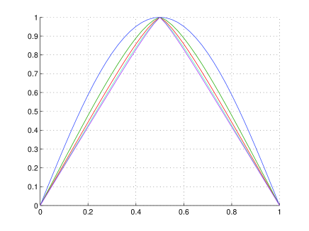
Example 4. Consider the eigenvalue problem for the $p$-Laplace operator

$$\mathrm{div}(|Dw_{1}|^{p-2}Dw_{1})+\lambda_{1}|w_{1}|^{p-2}w_{1}=0.$$

This example does not fit exactly in the framework of this paper since the operator is not uniformly elliptic. However, the following formula

$$\lambda_{p,h}:=-\inf_{\varphi>0}\sup_{y\in\Omega_{h}}\left\{\frac{F_{h,p}[\varphi](y)}{\varphi(y)^{p-1}}\right\}$$

where $F_{h,p}$ is a finite-difference approximations of $F_{p}$ produces a good approximation of the principal eigenvalue of the $p$-Laplace operator in the interval $(a,b)$ whose exact value is given by

$$\sqrt[p]{\lambda_{p}}=\frac{2\pi\sqrt[p]{p-1}}{(b-a)p\sin(\frac{\pi}{p})}.$$

In Table 4.4 we report the approximation error and the corresponding order of convergence for the principal eigenvalue of the $p$-Laplace operator for $p=4$ (in this case $\lambda_{4}\approx 73.0568$).

$h$	$Err(\lambda_{4})$	$Order(\lambda_{4})$
$1.00\cdot 10^{-1}$	$2.6770$
$5.00\cdot 10^{-2}$	$0.6210$	2.1079
$2.50\cdot 10^{-2}$	$0.1457$	2.0912
$1.25\cdot 10^{-2}$	$0.0347$	2.0724
$6.25\cdot 10^{-3}$	$0.0083$	2.0581

Table 4.4: Space step(first column), eigenvalue error (second column), convergence order (third column) for the $p$-Laplace operator with $p=4$

It is also known (see [16]) that if $\Omega$ is a ball, the eigenfunction $w_{p}$ corresponding to the eigenvalue $\lambda_{p}$ converges for $p\to\infty$ to $d(x,\partial\Omega)$. In Figure 4.2, we draw approximations of $w_{p}$ computed by the scheme for various values of $p$ and we observe the convergence of these functions to $d(x,\{0,1\})$ for $p$ increasing, as expected by the theory.

Figure 4.2: Approximate eigenfunction $u_{p,h}$ for $p=2,4,6,8,10$ and $h=10^{-3}$

4.2 Discretization in higher dimension.

We now consider the eigenvalue problem in ${\mathbb{R}}^{N}$. Arguing as in the 1-dimensional case we write

$$\small{\begin{split}\frac{F_{h}[u](x)}{u(x)}={{\cal F}}\Big{(}x,1,&\left\{\frac{u(x+hy)-u(x-hy)}{2h|y|u(x)}\right\}_{y\in Y},\left\{\frac{u(x+hy)+u(x-hy)}{h^{2}|y|^{2}u(x)}-\frac{2}{h^{2}}\right\}_{y\in Y}\Big{)}\end{split}}$$ (4.3)

for $i=1,\dots,N_{h}$ and $F_{h}$ defined as in (3.1), $Y$ the stencil and ${N_{h}}$ the cardinality of $\Omega_{h}$. Hence if the function ${\cal F}(x,z,\{q_{y}\}_{y\in Y},\{s_{y}\}_{y\in Y})$ is linear or more generally convex in the variables $q_{y}$ and $s_{y}$, $y\in Y$, then the computation of the principal eigenvalue $\lambda_{1,h}$ is equivalent to the minimization with respect to the vector $U\in{\mathbb{R}}^{N_{h}}$ of the convex function ${\cal G}:{\mathbb{R}}^{N_{h}}\to{\mathbb{R}}$ obtained by taking the maximum with respect to $x\in\Omega_{h}$ in (4.3). Therefore this problem can be solved by means of some standard algorithms in convex optimization.Example 5. Consider the problem

$$\left\{\begin{array}[]{ll}\Delta w+\lambda w=0&x\in(0,1)^{2},\\ w(x)=0&x\in\partial((0,1)^{2}).\end{array}\right.$$

The eigenvalue and the corresponding eigenfunction are given by

$$\lambda_{1}=2\pi^{2},\qquad w(x_{1},x_{2})=\sin(\pi x_{1})\sin(\pi x_{2})$$

(the eigenfunctions are normalized by taking $\|w\|_{\infty}=\|w_{h}\|_{\infty}=1$). We use a standard five-point formula for the discretization of the Laplacian. In Table 4.5, we compare the exact solution with the approximate one obtained by the scheme (4.1). We report the approximation error for $\lambda_{1}$ and $w_{1}$ (in $L^{\infty}$-norm and $L^{2}$-norm) and the order of convergence for $\lambda_{1}$. We can observe an order of convergence close to $2$ for $\lambda_{1}$ and therefore equivalent to one obtained by discretization of the Rayleigh quotient via finite elements, see [10].

$h$	$Err(\lambda_{1})$	$Order(\lambda_{1})$	$Err_{\infty}(w)$	$Err_{2}(w)$
$2.00\cdot 10^{-1}$	$0.4469$		$0.0801$	$0.2256$
$1.00\cdot 10^{-1}$	$0.1338$	$1.7397$	$0.0203$	$0.1137$
$5.00\cdot 10^{-2}$	$0.0368$	$1.8629$	$0.0056$	$0.0590$
$2.50\cdot 10^{-2}$	$0.0097$	$1.9297$	$0.0015$	$0.0301$

Table 4.5: Space step (first column), eigenvalue error (second column), convergence order (third column), eigenfunction error in $L^{\infty}$ (fourth column), eigenfunction error in $L^{2}$ (last column)

Example 6. We consider the eigenvalue problem for the Ornstein-Uhlenbeck operator

$$\Delta w-x\cdot Dw+\lambda w=0,\qquad x\in(-1,1)^{2}$$

with homogeneous boundary conditions. The eigenvalue and the corresponding eigenfunction are given by

$$\lambda_{1}=4,\qquad w(x_{1},x_{2})=(1-x_{1}^{2})(1-x_{2}^{2}),$$

with the eigenfunctions normalized by taking $\|w\|_{\infty}=\|w_{1,h}\|_{\infty}=1$. The Laplacian is discretized by a five-point formula. In Table 4.6, we report the approximation error for $\lambda_{1}$ and the corresponding order of convergence.

$h$	$Err(\lambda_{1})$	$Order(\lambda_{1})$
$4.00\cdot 10^{-1}$	$0.1524$
$2.00\cdot 10^{-1}$	$0.0392$	$1.9592$
$1.00\cdot 10^{-1}$	$0.0103$	$1.9250$
$5.00\cdot 10^{-2}$	$0.0027$	$1.9580$

Table 4.6: Space step (first column), eigenvalue error (second column), convergence order (third column)

References

• [1] S.N. Armstrong, The Dirichlet problem for the Bellman equation at resonance. J. Differential Equations 247 (2009), 931-955.
• [2] I. Babuska, J. E. Osborn, Finite element-Galerkin approximation of the eigenvalues and eigenvectors of selfadjoint problems. Math. Comp. 52 (1989), 275-297.
• [3] G. Barles, P. Souganidis, Convergence of approximation schemes for fully nonlinear second order equations. Asymptotic Anal. 4 (1991), 271-283.
• [4] A. Bensoussan, Perturbation methods in optimal control. Wiley/Gauthier-Villars Series in Modern Applied Mathematics. John Wiley & Sons, Ltd., Chichester; Gauthier-Villars, Montrouge, 1988.
• [5] H. Berestycki, I. Capuzzo Dolcetta, A. Porretta, L. Rossi, Maximum Principle and generalized principal eigenvalue for degenerate elliptic operators. J. Math. Pures Appl. 103 (2015), no. 5, 1276-1293.
• [6] H. Berestycki, L. Nirenberg, S.R.S. Varadhan, The principal eigenvalue and maximum principle for second-order elliptic operators in general domains. Comm. Pure Appl. Math. 47 (1994), no. 1, 47–92.
• [7] R.J. Biezuner, G. Ercole, E.D. Martins, Computing the first eigenvalue of the p-Laplacian via the inverse power method. J. Funct. Anal. 257 (2009), no. 1, 243-270.
• [8] I.Birindelli, F. Demengel, First eigenvalue and maximum principle for fully nonlinear singular operators. Adv. Differential Equations 11 (2006), no. 1, 91-119.
• [9] I. Birindelli, F. Leoni, Symmetry minimizes the principal eigenvalue: an example for the Pucci’s sup operator. Math. Res. Lett. 21 (2014), no. 5, 953 - 967.
• [10] D. Boffi, Finite element approximation of eigenvalue problems. Acta Numer. 19 (2010), 1-120.
• [11] J. Busca, M. Esteban, A. Quaas, Nonlinear eigenvalues and bifurcation problems for Pucci’s operator. Ann. Inst. H. Poincaré Anal. Non Linéaire 22 (2005), no. 2, 187-206.
• [12] M.D. Donsker, S.R.S. Varadhan, On the principal eigenvalue of second-order elliptic differential operators, Comm. Pure Appl. Math. 29 (1976), 595-621.
• [13] D. Gomes, A. Oberman, Computing the effective Hamiltonian using a variational approach. SIAM J. Control Optim. 43 (2004), 792–812.
• [14] W. Huang, Sign-preserving of principal eigenfunctions in P1 finite element approximation of eigenvalue problems of second-order elliptic operators. J. Comput. Phys. 274 (2014), 230-244.
• [15] H.Ishii, N.Ikoma, Eigenvalue problem for fully nonlinear second-order elliptic PDE on balls. Ann. Inst. H. Poincaré Anal. Non Linéaire 29 (2012), 783-812.
• [16] P. Juutinen, P. Lindqvist, J.J. Manfredi, The $\infty$-eigenvalue problem. Arch. Ration. Mech. Anal. 148 (1999), no. 2, 89-105.
• [17] H.J. Kuo, N. Trudinger, Linear elliptic difference inequalities with random coefficients. Math. Comp. 55 (1990), no. 191, 37-53.
• [18] H.J. Kuo, N. Trudinger, Discrete methods for fully nonlinear elliptic equations. SIAM J. Numer. Anal. 29 (1992), 123–135.
• [19] M. G. Krein, M. A. Rutman, Linear operators leaving invariant a cone in a Banach space. Amer. Math. Soc. Translation (1950), no. 26, 128 pp.
• [20] P.-L. Lions, Bifurcation and optimal stochastic control. Nonlinear Anal. 7 (1983), 177-207.
• [21] C. Pucci, Maximum and minimum first eigenvalues for a class of elliptic operators. Proc. Amer. Math. Soc. 17 (1966), 788-795.
• [22] H. F. Weinberger,Variational methods for eigenvalue approximation. Conference Board of the Mathematical Sciences Regional Conference Series in Applied Mathematics, no. 15, SIAM, Philadelphia, 1974.