On the limit zero distribution of type I Hermite–Padé polynomials

Abstract.

In this paper are discussed the results of new numerical experiments on zero distribution of type I Hermite–Padé polynomials of order $n=200$ for three different collections of three functions $[1,f_{1},f_{2}]$. These results are obtained by the authors numerically and do not match any of the theoretical results that were proven so far. We consider three simple cases of multivalued analytic functions $f_{1}$ and $f_{2}$, with separated pairs of branch points belonging to the real line. In the first case both functions have two logarithmic branch points, in the second case they both have branch points of second order, and finally, in the third case they both have branch points of third order.

All three cases may be considered as representative of the asymptotic theory of Hermite–Padé polynomials. In the first two cases the numerical zero distribution of type I Hermite–Padé polynomials are similar to each other, despite the different kind of branching. But neither the logarithmic case, nor the square root case can be explained from the asymptotic point of view of the theory of type I Hermite–Padé polynomials.

The numerical results of the current paper might be considered as a challenge for the community of all experts on Hermite–Padé polynomials theory.

Bibliography: [79] items.

Figures: 72 items.

Keywords: Hermite–Padé polynomials, limit zero distribution, equilibrium problem, $S$-compact set, convergence in capacity.

1. Introduction

In this article, we are concerned with the general problem of the limit zero distribution (LZD) of type I Hermite–Padé (HP) polynomials for the collection of $m$ function $[f_{0}\equiv 1,f_{1},\dots,f_{m-1}]$, $m\geqslant 3$, where $f_{1},\dots,f_{m-1}$ are multivalued analytic functions, each one having a finite set of branch points on the Riemann sphere $\overline{\mathbb{C}}$; the reader is referred at first to the basic surveys [52], [69], and also [27], [49], [3]. Up to the end of the paper, suppose that the functions $f_{0}\equiv 1,f_{1},\dots,f_{m-1}$ are rationally independent (over the field $\mathbb{C}(z)$).

We restrict our attention to the case of the collection of three functions, in other words, to the case $m=3$. Let us recall some basic notions from the HP polynomials theory (see [52], [69]).

Suppose that two functions $f_{1}$ and $f_{2}$ are given by convergent power series at the infinity point $z=\infty$. For a fixed number $n\in\mathbb{N}$, the type I HP polynomials $Q_{n,0},Q_{n,1},Q_{n,2}$ of degree $\leqslant{n}$, $Q_{n,j}=Q_{n,j}(z;f_{1},f_{2})\in\mathbb{P}_{n}$, $\mathbb{P}_{n}:=\mathbb{C}_{n}(z)$, $j=0,1,2$, not all $Q_{n,j}\equiv 0$, are defined in such a way that the following basic relation holds true:

$$R_{n}(z):=(Q_{n,0}\cdot 1+Q_{n,1}f_{1}+Q_{n,2}f_{2})(z)=O\left(\frac{1}{z^{2n+2}}\right),\quad z\to\infty.$$ (1)

It is well known that such polynomials $Q_{n,j}$ always exist and in the “generic case” they are unique up to a suitable normalization (see [52], [69], [49], [38]).

To be more precise, we treat here, from numerical point of view, three different pairs of Markov-type functions: $f_{1},f_{2}$, $g_{1},g_{2}$ and $h_{1},h_{2}$.

Recall that a function $f\in\mathscr{H}(\infty)$ is a Markov-type function if $f(z)=\widehat{\mu}(z)+\operatorname{const}$, where $\widehat{\mu}$ is the Cauchy transform of a positive Borel measure, with support $\operatorname{supp}\mu\Subset\mathbb{R}$ (a compact subset of the real line $\mathbb{R}$),

$$\widehat{\mu}(z):=\int\frac{d\mu(x)}{z-x},\quad z\not\in\operatorname{supp}\mu.$$ (2)

Up to the end of the paper, a support of a Markov-type function $f=\widehat{\mu}+\operatorname{const}$ means the support of the corresponding measure $\mu$.

Let $E_{1}:=[a_{1},a_{2}]=[-1,a]$, $E_{2}:=[b_{1},b_{2}]=[-a,1]$, where $a\in(0,1)$ is a real parameter. Hence both segments $E_{1}$ and $E_{2}$ are overlapping, $E_{1}\cap E_{2}=[-a,a]\not=\varnothing$.

Case 1.

Let

$$f_{1}(z) :=\int_{-1}^{a}\frac{dx}{z-x}=\log\frac{z-a}{z+1},\quad z\notin E_{1},$$ (3)

$$f_{2}(z) :=\int_{-a}^{1}\frac{dx}{z-x}=\log\frac{z-1}{z+a},\quad z\notin E_{2}.$$ (4)

We take the main branch of the logarithmic function in (3) and (4), in the sense that

$$\log\frac{z-a}{z+1},\ \log\frac{z-1}{z+a}\approx\log{1}=0,\quad\text{as}\quad z\to\infty.$$

Case 2.

Let

$$g_{1}(z) :=\left(\frac{z-a}{z+1}\right)^{1/2}=\frac{1}{\pi}\int_{-1}^{a}\sqrt{\frac{a-x}{x+1}}\frac{dx}{x-z}+1,\quad z\notin E_{1},$$ (5)

$$g_{2}(z) :=\left(\frac{z-1}{z+a}\right)^{1/2}=\frac{1}{\pi}\int_{-a}^{1}\sqrt{\frac{1-x}{x+a}}\frac{dx}{x-z}+1,\quad z\notin E_{2}.$$ (6)

We take such a branch of the $(\cdot)^{1/2}$ function, that $g_{1}(z),g_{2}(z)\to 1$ as $z\to\infty$, and under the square root function $\sqrt{\,\cdot\,}$ we mean the “arithmetic square root function”, that is $\sqrt{x^{2}}=x$ for $x\in\mathbb{R}_{+}$.

Case 3.

Let

$$h_{1}(z) :=\left(\frac{z-a}{z+1}\right)^{1/3},\quad z\notin E_{1},$$ (7)

$$h_{2}(z) :=\left(\frac{z-1}{z+a}\right)^{1/3},\quad z\notin E_{2}.$$ (8)

We take such a branch of the $(\cdot)^{1/3}$ function, that $h_{1}(z),h_{2}(z)\to 1$ as $z\to\infty$, and, in what follows, under the cubic root function $\sqrt[3]{\,\cdot\,}$ we mean the “arithmetic cubic root function”, that is $\sqrt[3]{x^{3}}=x$ for $x\in\mathbb{R}_{+}$.

Clearly, all three functions $f_{j},g_{j},h_{j}$, $j=1,2,3$ are Markov-type functions. But since $a\in(0,1)$, we have $E_{1}\cap E_{2}=[-a,a]\neq\varnothing$ and $E_{1}\neq E_{2}$. Hence, all three pairs $f_{1},f_{2}$, $g_{1},g_{2}$ and $h_{1},h_{2}$ are neither an Angelesco, nor a Nikishin system (see [52], [21], [49], [26], [27], [4]). Thus so far, not even one theorem of general type is known, which predicts the LZD of type I HP polynomials for the three collections of multivalued analytic functions $[1,f_{1},f_{2}]$, $[1,g_{1},g_{2}]$ and $[1,h_{1},h_{2}]$, that were introduced above. Hence, the numerical results that are presented in this paper should be explained from theoretical point of view by the forthcoming papers.

Since $a$ is a parameter, we actually have three families of Markov-type functions: $\mathscr{T}=\{f_{1}=f_{1}(z;a),\ f_{2}=f_{2}(z;a),\ a\in(0,1)\}$, $\mathscr{G}=\{g_{1}=g_{1}(z;a),\ g_{2}=g_{2}(z;a),\ a\in(0,1)\}$, and $\mathscr{H}=\{h_{1}=h_{1}(z;a),\ h_{2}=h_{2}(z;a),\ a\in(0,1)\}$. Thus, for a fixed $n\in\mathbb{N}$, we have three families of HP polynomials defined by the basic relation (1). To distinguish between Case 1, Case 2, and Case 3, we introduce new notations for the HP polynomials for the collections of three functions $[1,g_{1},g_{2}]$ and $[1,h_{1},h_{2}]$. We set $P_{n,0},P_{n,1},P_{n,2}\in\mathbb{P}_{n}\setminus\{0\}$ for the HP polynomials corresponding to the collection $[1,g_{1},g_{2}]$,

$$(P_{n,0}\cdot 1+P_{n,1}g_{1}+P_{n,2}g_{2})(z)=O\left(\frac{1}{z^{2n+2}}\right),\quad z\to\infty,$$ (9)

and $U_{n,0},U_{n,1},U_{n,2}\in\mathbb{P}_{n}\setminus\{0\}$ for the HP polynomials corresponding to the collection $[1,h_{1},h_{2}]$,

$$(U_{n,0}\cdot 1+U_{n,1}h_{1}+U_{n,2}h_{2})(z)=O\left(\frac{1}{z^{2n+2}}\right),\quad z\to\infty.$$ (10)

Notice that for each value of the parameter $a\in(0,1)$ the supports of the two Markov-type functions $f_{j}$ and $g_{j}$, $j=1,2$, coincide with each other, but the types of the corresponding branch points are of different nature. It is worth noting that in each pair $f_{1},f_{2}$ and $g_{1},g_{2}$, the branch points are separated from each other (cf. [54], [2]). But since for each $a\in(0,1)$, $E_{1}\cap E_{2}\neq\varnothing$, $E_{1}\not\subset E_{2}$, and $E_{2}\not\subset E_{1}$, the system $f_{1},f_{2}$ is neither an Angelesco, nor a Nikishin system. The same is true for the systems $g_{1},g_{2}$ and $h_{1},h_{2}$.

In all of the numerical experiments discussed in the present paper, we set $n=200$ (see (1)). We also fix the set of values of parameter $a$ as to be $a=0.2;0.4;0.625;0.73;0.8$.

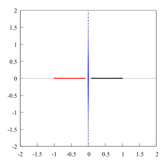
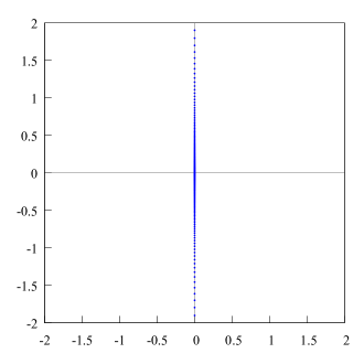
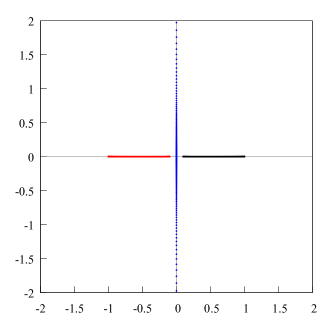
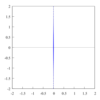
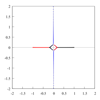
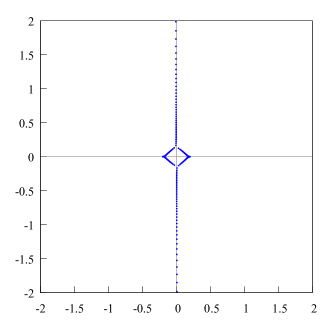
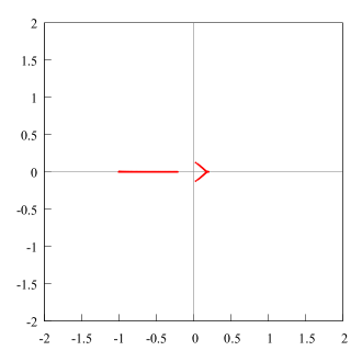
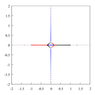
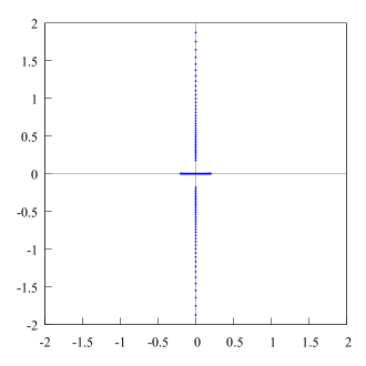
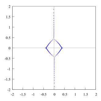
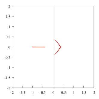
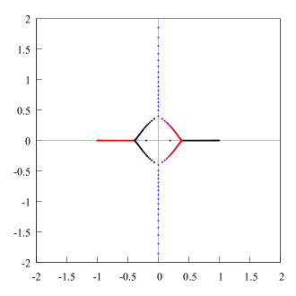
At first we set $a=-0.1$ (and keep $n=200$). Clearly, that value of $a$ is out of the range of $(0,1)$. But the reason is that for $a=-0.1$ all three pairs $f_{1},f_{2}$, $g_{1},g_{2}$ and $h_{1},h_{2}$ form Angelesco systems, since $E_{1},E_{2}\subset\mathbb{R}$ and $E_{1}\cap E_{2}=\varnothing$. On Fig. 9 and Fig. 11 zeros of HP polynomials $Q_{200,j}$ and $P_{200,j}$, $j=0,1,2$, are plotted. The numerical distribution of the zeros of the HP polynomials are similar in both cases and do not depend on the different type of branching of the functions $f_{1},f_{2}$ and $g_{1},g_{2}$ at the points $z=\pm 1,\pm a$. The reason is as follows. All these numerical results are in full agreement with the general theory of limit zero distribution (LZD) for HP polynomials in the Angelesco case (see [21], [26], [4]; in these papers the case of type II HP polynomials was considered, but it is well known that in the Angelesco’s case there is a direct connection between LZD of type I and type II HP polynomials). Since the sizes of the supports of Markov-type functions $f_{1}$ and $f_{2}$ (and $g_{1}$, $g_{2}$ as well) are equal, the phenomena of the so-called “pushing of the charge” is absent in the case $a=-0.1$. It is in full agreement also with the general theory (see [30], [1], [21]). From Fig. 9, Fig. 10, Fig. 11, Fig. 12 follows, that the zeros of HP polynomials $Q_{200,1}$ and $Q_{200,2}$ (and $P_{200,1}$, $P_{200,2}$ as well) are located on the segments $E_{1}$ and $E_{2}$, respectively. But the zeros of $Q_{200,0}$ (and $P_{200,0}$ respectively) are located on the imaginary axis. Thus in some sense the zeros of $Q_{200,0}$ “intend to separate” the zeros of $Q_{200,1}$ and $Q_{200,2}$ from each other. Again this result is in good agreement with the well known LZD of type I HP polynomials in the Angelesco case (see, e.g. [54]). To finish the analysis of the case $a=-0.1$, we emphasize that in this case all numerical results are in good agreement with the general theory of HP polynomials. Thus, it is reasonable to consider all numerical results for $a=0.2;0.4;0.625;0.73;0.8$ as to be trustable.

We describe in short the numerical experiments.

We set the parameter $a$ to be $0.2;0.4;0.625;0.73;0.8$, and for each value of $a$ we find numerically the zeros of HP polynomials $Q_{200,j}(z;a)$, $P_{200,j}(z;a)$ and $U_{200,j}(z;a)$, $j=0,1,2$, respectively. Thus we obtain a “series” of numerical experiments for the different values of the parameter $a$. By the reasons mentioned above, it is meaningful to consider all these numerical results as trustable, and hence we can analyze them from a theoretical point of view.

Before laying out in details the discussion and the analysis of the results of the numerical experiments (see subsection §4.3), we recall basic general facts about Padé approximants convergence theory (PA-theory). For this purpose, we provide in the next sections §2 and §3 a survey for the most important results of PA convergence theory, which is intended to make more clear the mathematical essence of the numerical results presented in the current paper.

2. Classical Padé approximants (or $J$-fractions) convergence theory

2.1. Stahl’s $S$-curve and Stahl’s limit zero-pole distribution theorem in classical Padé approximants theory

The basic general results of PA-theory are of two types. The first type is concerned with the limit zero distribution of Padé polynomials for multivalued analytic functions with a finite set of branch points on the Riemann sphere $\overline{\mathbb{C}}$. Commonly, these results are referred to as “weak asymptotics of PA”. The second type of results are devoted to the so-called “strong asymptotics of PA”.

The problem of first type was originally stated in a formal way by J. Nuttall (see [51] and the review [52]) at the beginning of 1970’s, and for the classical (“one-point”) Padé approximants the problem was completely solved by H. Stahl [64]–[68] in the middle of 1980’s (see also [71]).

The second type problem was also initiated by Nuttall (see [50], [52], [53], [55] and also [31, § 2, Conjecture 1]). Recently were obtained strong results in this direction (see [73], [7], [44]). However, generally the problem is still far from being solved even for the classical PA. We explain the main reason for this situation. The “strong asymptotics theory” is a far and deep generalization of the classical Bernstein–Szegő asymptotic theory for the ordinary polynomials, orthogonal on the unit segment $\Delta:=[-1,1]$ and related to the general case of non-Hermitian orthogonal polynomials (see [77], [10], [52, Section 1 and Section 6], [55], the paper by H. Widom [79], as well).

Given a germ $f$ of a multivalued analytic function $f$ with a finite number of branch points, the seminal Stahl Theorem gives a complete answer to the problem of limit zero-pole distribution of the classical PA to $f$. Stahl Theorem is of a quite general character. It not only admits multivalued functions with a finite number of branch points on the Riemann sphere, but also multivalued analytic functions with a singular set of zero (logarithmic) capacity. The keystone of Stahl theory [64]–[68] is the existence of a unique (up to a compact set of zero capacity) maximal domain for the given at the point $z=\infty$ multivalued function $f$. The so-called “maximal domain” of holomorphy of $f$ is a domain $D=D(f)\ni\infty$, such that the given germ $f$ can be continued as holomorphic (analytic and single-valued) function from a neighborhood of the infinity point $z=\infty$ to $D$ (the function $f$ can be continued analytically along each path that belongs in to $D$). “Maximal” means that $\partial{D}$ is of “minimal capacity” among all compact sets $\partial{G}$, such that $G$ is a domain, $\infty\in G$ and $f\in\mathscr{H}(G)$. Such “maximal” domain $D$ is unique (up to a compact set of zero capacity). The compact set $S=S(f):=\partial{D}$ is now called “Stahl’s compact set” or “Stahl’s $S$-compact set”, and $D$ is called “Stahl’s domain”. The crucial properties of $S$ for the Stahl theory to be true are the following: the complement $D=\overline{\mathbb{C}}\setminus{S}$ is a domain, $S$ consists of a finite number of analytic arcs (in fact, the union of the closures of the critical trajectories of a quadratic differential), and, finally, $S$ possesses the so-called property of “symmetry”, that is,

$$\frac{\partial g_{D}(z,\infty)}{\partial n^{+}}=\frac{\partial g_{D}(z,\infty)}{\partial n^{-}},\quad z\in S^{0},$$ (11)

where $g_{D}(z,\infty)$ is Green’s function for the domain $D$, with the logarithmic singularity at the point $z=\infty$, $S^{0}$ is the union of all open arcs of $S$ (which closures constitute $S$, that is $S\setminus S^{0}$ is a finite set), and $\partial n^{+}$ and $\partial n^{-}$ are the inner (with respect to $D$) normal derivatives of $g_{D}(z,\infty)$ at a point $z\in S^{0}$ from the opposite sides of $S^{0}$.

Given a finite set $\Sigma\subset\overline{\mathbb{C}}$, $\#\Sigma<\infty$, let $\mathscr{A}(\overline{\mathbb{C}}\setminus\Sigma)$ be the set of all functions analytic in the domain $\overline{\mathbb{C}}\setminus\Sigma$. Let $\mathscr{A}^{0}(\overline{\mathbb{C}}\setminus\Sigma):=\mathscr{A}(\overline{\mathbb{C}}\setminus\Sigma)\setminus\mathscr{H}(\overline{\mathbb{C}}\setminus\Sigma)$, i.e. for a fixed $\Sigma$ a function $f$ is from the set $\mathscr{A}^{0}(\overline{\mathbb{C}}\setminus\Sigma)$ if it is a multivalued analytic function in the domain $\overline{\mathbb{C}}\setminus\Sigma$, but not a holomorphic function in $\overline{\mathbb{C}}\setminus\Sigma$ ($f$ is analytic, but not single-valued).

Let $\Sigma=\Sigma_{f}=\{a_{1},\dots,a_{p}\}$, $\#\Sigma=p<\infty$, be the set of all branch points of $f$, i.e. $f\in\mathscr{A}(\overline{\mathbb{C}}\setminus\Sigma)\setminus\mathscr{H}(\overline{\mathbb{C}}\setminus\Sigma)=:\mathscr{A}^{0}(\overline{\mathbb{C}}\setminus\Sigma)$. Clearly, if $\Sigma_{f}=\{-1,1\}$, then Stahl’s compact set (with respect to the infinity point) $S=[-1,1]$.

The properties of the compact set $S$ described above are crucial for the validness of Stahl Theorem.

We recall some basic notations from the general PA-theory.

Let there be given a function $f\in\mathscr{A}^{0}(\overline{\mathbb{C}}\setminus\Sigma)$, which is holomorphic at the infinity point, $f\in\mathscr{H}(\infty)$. To be more precise, suppose we are given a convergent power series, i.e. a germ,

$$f=\sum_{k=0}^{\infty}\frac{c_{k}}{z^{k+1}},$$ (12)

and the corresponding analytic function $f\in\mathscr{A}^{0}(\overline{\mathbb{C}}\setminus\Sigma)$, where $\#\Sigma<\infty$. For a positive Borel measure $\mu$ with a compact support $\operatorname{supp}(\mu)\Subset\overline{\mathbb{C}}$, denote by $V^{\mu}(z)$ the logarithmic potential of $\mu$, that is:

$$V^{\mu}(z):=\int_{\operatorname{supp}\mu}\log\frac{1}{|z-\zeta|}\,d\mu(\zeta).$$

Given a number $n\in\mathbb{N}$, let $P_{n,0},P_{n,1}\in\mathbb{C}_{n}(z)$, $P_{n,1}\not\equiv 0$, be the Padé polynomials (at the infinity point) of the function $f$. We recall that

$$R_{n}(z):=(P_{n,0}+P_{n,1}f)(z)=O\left(\frac{1}{z^{n+1}}\right),\quad z\to\infty.$$ (13)

The polynomials $P_{n,0},P_{n,1}$ are not unique, but the ratio $P_{n,0}/P_{n,1}$ is uniquely determined by the relation (13). The rational function $[n/n]_{f}:=-P_{n,0}/P_{n,1}$ is called the diagonal Padé approximant of order $n$ (or the $n$-diagonal Padé approximant) of the function $f$ (at the infinity point), and $R_{n}$ is the remainder function of the Padé approximant.

Given an arbitrary polynomial $Q\in\mathbb{C}(z)$, $Q\not\equiv 0$, denote by

$$\chi(Q):=\sum_{\zeta:Q(\zeta)=0}\delta_{\zeta}$$

the associated zero counting measure of $Q$ (as usual, $\delta_{\zeta}$ denotes the Dirac measure concentrated at the point $\zeta\in\overline{\mathbb{C}}$).

One of the main results of Stahl theory [64]–[68] is

Stahl Theorem (H. Stahl, see [67], [71]).

Let $f\in\mathscr{H}(\infty)$, $f\in\mathscr{A}^{0}(\overline{\mathbb{C}}\setminus\Sigma$), $\#\Sigma<\infty$. Let $D=D(f)$ be Stahl’s “maximal” domain for $f$, $S=\partial{D}$ – Stahl’s compact set, $[n/n]_{f}=-P_{n,0}/P_{n,1}$ – the $n$-diagonal Padé approximant to the function $f$. Then the following statements are valid:

1) there exists LZD of Padé polynomials $P_{n,j}$, $j=0,1$, namely,

$$\frac{1}{n}\chi(P_{n,j})\overset{*}{\longrightarrow}\lambda,\quad\text{as}\quad n\to\infty,\quad j=0,1,$$ (14)

where $\lambda=\lambda_{S}$ is a unique probability equilibrium measure of the compact set $S$;

2) the $n$-diagonal Padé approximants converge in capacity to the function $f$ inside the domain $D$,

$$[n/n]_{f}(z)\overset{\operatorname{cap}}{\longrightarrow}f(z),\quad n\to\infty,\quad z\in D;$$ (15)

3) the rate of the convergence in (15) is completely characterized by the equality

$$\bigl{|}(f-[n/n]_{f})(z)\bigr{|}^{1/n}\overset{\operatorname{cap}}{\longrightarrow}e^{-2g_{D}(z,\infty)},\quad n\to\infty,\quad z\in D.$$ (16)

Remark 1.

In item 1), $\lambda_{S}$ is the unique probability equilibrium measure of the compact set $S$, that is $V^{\lambda_{S}}(z)\equiv\gamma_{S},\,z\in S$, where $V^{\lambda_{S}}(z)=-\int\log|z-\zeta|\,d\lambda_{S}(\zeta)$ is the logarithmic potential of the measure $\lambda_{S}$, $\gamma_{S}$ is the Robin constant for $S$. The notation “$\overset{*}{\longrightarrow}$” stands for convergence of measures in the weak-star topology. The notation “$\overset{\operatorname{cap}}{\longrightarrow}$” in items 2) and 3) means convergence in capacity inside (on compact subsets of) the domain $D$.

As it is basely known, $g_{D}(z,\infty)\equiv\gamma_{S}-V^{\lambda_{S}}(z)$. From here it follows immediately, that the $S$-property (11) may be written in an equivalent form (cf. (25)), namely

$$\frac{\partial V^{\lambda}}{\partial n^{+}}(z)=\frac{\partial V^{\lambda}}{\partial n^{-}}(z),\quad z\in S^{0}.$$ (17)

Remark 2.

Let $P^{*}_{n,j}$, $j=0,1$, be the monic Padé polynomials. Then the statement of item 1) is equivalent to the following:

$$\bigl{|}P^{*}_{n,j}(z)\bigr{|}^{1/n}\overset{\operatorname{cap}}{\longrightarrow}e^{-V^{\lambda_{S}}(z)},\quad n\to\infty,\quad z\in D,\quad j=0,1.$$ (18)

Similarly, denote by $R^{*}_{n}(z)$ the normalized remainder function,

$$R^{*}_{n}(z)=\frac{1}{z^{n+1+\ell_{n}}}+\dotsb,\quad z\to\infty,$$

where $\ell_{n}\in\mathbb{Z}$, $\ell_{n}=o(n)$ as $n\to\infty$. Then the statement of item 3) is equivalent to the following:

$$\bigl{|}R^{*}_{n}(z)\bigr{|}^{1/n}\overset{\operatorname{cap}}{\longrightarrow}e^{-g_{D}(z,\infty)},\quad n\to\infty,\quad z\in D.$$ (19)

Let $\Sigma_{f}=\{-1,1\}$. Clearly, in this $S=[-1,1]$. Hence, for the case of a general multivalued analytic function $f\in\mathscr{A}^{0}(\overline{\mathbb{C}}\setminus\Sigma_{f})$, $\#\Sigma_{f}<\infty$, the associated (with the function $f$) Stahl’s compact set $S$ should be considered as a natural replacement of the unit segment $\Delta=[-1,1]$, which is the main object in the classical Bernstein–Szegő asymptotic theory. Recall that the classical Bernstein–Szegő formula of strong asymptotics for polynomials, orthogonal on the segment $\Delta$ with respect to a weight $\rho$ defined on $\Delta$ and “smooth” enough, is presented in terms of Szegő function, associated with $\rho$, and the “mapping” function $\varphi(z)=z+(z^{2}-1)^{1/2}$, associated with $\Delta$. Viewing Stahl Theorem, it is natural to conjecture, that in the formula of strong asymptotics of Padé polynomials $P_{n,j}$ Stahl’s compact set $S$ should appear in a natural way, but not the segment $\Delta$ or the finite union of the real segments (see [10], [79], [52], [53, Conjecture 1], [7], [31, Conjecture 2]).

The existence of Stahl’s $S$-curve for an arbitrary multivalued analytic function with a finite set of singular points, on one hand, and Stahl Theorem of the LZD of Padé polynomials, on the other, should play a crucial role in the forthcoming development of the theory of the strong asymptotics of Padé polynomials, associated with a multivalued analytic function, and the corresponding theory of strong convergence of Padé approximants (cf. [28], [7]).

It is worth noting that, in general, the property of a symmetry (in other words, $S$-property of type (11), (25), see [61, formula (11)]) gives rise to a local analogue of complex conjugation operation and to the method of the construction of an associated two-sheeted or three-sheeted Riemann surface (see [71], [25], [61, § 6]).

In 1987 A. A. Gonchar and E. A. Rakhmanov [24] extended the original Stahl’s conception of symmetry (the $S$-curve conception) to the conception of “symmetry in the presence of an external field”. The general LZD-theorem of orthogonal polynomials was proven mainly by using the new notions in [24]; i.e., for polynomials orthogonal with respect to a variable weight (depending on the degree of the polynomial, see also [22]). This new concept of the “presence of an external field” offered Gonchar and Rakhmanov the chance to solve the well known “$1/9$-problem” (see [78], also Wolfram MathWorld: One-Ninth Constant, it is also known as “Varga’s constant”, see Wolfram MathWorld: Varga’s Constant). Finally, Stahl’s and Gonchar–Rakhmanov’s results gave rise to the so-called $\operatorname{GRS}$-method (Gonchar–Rakhmanov–Stahl-method), which solves the problem of LZD of generalized (non-Hermitian) quasi-orthogonal polynomials. The method itself consists of three steps.

First step: to state an appropriate theoretical potential extremal problem associated with the initial problem of LZD of Padé polynomials, and then proving the existence of an “extremal” compact set in some family of “admissible” compact sets.

Second step: to prove that the extremal compact set possesses the special property of “symmetry”, i.e., the set is a “weighted” $S$-curve, associated with the problem under consideration.

Third step: to establish that the LZD of the generalized orthogonal polynomials under question exists and coincides with the equilibrium probability measure (in the presence of the external field), which is concentrated on the weighted $S$-curve.

2.2. Strong asymptotics in classical Padé approximants theory

We give one of the possible forms of the strong asymptotics of Padé polynomials under the conditions of Stahl Theorem (cf. [31, § 2, Conjecture 1]). It is worth noting that in general (except for the case of genus zero) such a representation is not unique (see [19], [56], [39]). The reason is that there exist so-called spurious zeros of Padé polynomials, with behavior, as $n\to\infty$, that can be described in many ways.

Conjecture 1 (cf. [31], § 2, Conjecture 1).

Let $f\in\mathscr{H}(\infty)$ and $f\in\mathscr{A}^{0}(\overline{\mathbb{C}}\setminus\Sigma)$ for some finite set $\Sigma\subset\overline{\mathbb{C}}$. Let $D=D(f)$ be Stahl’s maximal domain associated with $f$, $S=S(f)=\partial{D}$ – the corresponding Stahl’s compact set for $f$, $\mathfrak{R}_{2}=\mathfrak{R}_{2}(f)$ – the canonical hyperelliptic two-sheeted Riemann surface associated with the compact set $S$, $\mathbf{z}=z^{(1,2)}=(z,\pm)\in\mathfrak{R}_{2}$ – an arbitrary point on the two-sheeted $\mathfrak{R}_{2}$, $\Psi_{n}(\mathbf{z})=\Psi_{n}(\mathbf{z};f)$ – Nuttall’s psi-function associated with $f$ and $\mathfrak{R}_{2}$. Then, after a suitable normalization of the Padé polynomials $P_{n,j}(z)=P_{n,j}(z;f)$, $j=0,1$, and the remainder function $R_{n}$, the following relations take place in capacity inside the domain $D$:

$$P_{n,j}(z) \overset{\operatorname{cap}}{=}\frac{(-1)^{j}}{f^{j}(z)}\Psi_{n}(z^{(1)})\bigl{(}1+o(1)\bigr{)},\quad n\to\infty,$$

$$R_{n}(z) \overset{\operatorname{cap}}{=}\frac{\Psi_{n}(z^{(2)})}{w(z^{(2)})}\bigl{(}1+o(1)\bigr{)},\quad n\to\infty,$$ (20)

where $w^{2}=H_{2g+2}(z)$, $H_{2g+2}\in\mathbb{C}_{2g+2}[z]$, is the equation that determines the hyperelliptic Riemann surface $\mathfrak{R}_{2}$ of genus $g$.

Conjecture 1 is based partly on Nuttall’s result from 1986 [53] (see also [44]) via Liouville–Steklov asymptotic method for the function $f$ of the special form

$$f(z)=\prod_{j=1}^{3}(z-a_{j})^{\alpha_{j}},\quad\sum_{j=1}^{3}\alpha_{j}=0,\quad\alpha_{j}\in\mathbb{C}\setminus\mathbb{Z},\quad f(\infty)=1$$ (21)

(cf. [53, § 5. Asymptotic Conjecture]).

Conjecture 1 was proven in some particular cases in [70], [73], [7], comp. also [52], [55], [6], [31].

In general, the problem of the strong asymptotics of Padé polynomials is still open and the state is as follows: there are only partial results about the subject, and all of them are based on the existence of Stahl’s compact set $S$ and the concepts associated with it, namely, the two-sheeted hyperelliptic Riemann surface and the corresponding Abelian integrals on it. The problem does not depend on the method used to produce the asymptotic formula: method of matrix Riemann–Hilbert boundary value problem, Liouville–Steklov method, method of the Nuttall’s singular integral equation. Ultimately, all these methods are based on the existence of Stahl’s $S$-curve.

3. Two-point Padé approximants (or $T$-fractions) convergence theory

Recently V. I. Buslaev [14] (see also [17], [15]) applied the $\operatorname{GRS}$-method in treating the multipoint PA of a multivalued analytic function with a finite set of branch points. Buslaev [14] proved an analogue of the classical Stahl Theorem, furthermore, he discovered some special features of the multipoint PA. In particular, for the case of two-point PA, say at the points $z=0$ and $z=\infty$, he was the first, who found that in the “generic case” the weighted $S$-curve, associated with this problem, partitions the Riemann sphere in an “optimal way” into two domains $D_{0}\ni 0$ and $D_{\infty}\ni\infty$. At the same time, it was well known that the $\operatorname{GRS}$-method does not work in such a disconnected situation. In the case of multipoint ($m$-point) PA the situation is even more complicated, since it should be treated as a problem of an optimal partition of the Riemann sphere into $m$ domains. Nevertheless, the suitable generalization and improvement of the original version of the $\operatorname{GRS}$-method to this situation was given by Buslaev in [14]. This generalization provided Buslaev the opportunity to extend Stahl theory to multipoint PA for multivalued analytic functions. In fact, Buslaev made a new step towards the development of the $\operatorname{GRS}$-method in order to extend it to the disconnected case. Ultimately, it made the $\operatorname{GRS}$-method much more powerful than it was before.

3.1. Buslaev’s $S$-curve and Buslaev’s limit zero-pole distribution theorem in two-point Padé approximants theory

Let us discuss in short the case of multipoint PA and Buslaev Theorem. The original version of Buslaev Theorem is of general kind, since it deals with $m$-point PA. To be more precise, given a set of $m$ distinct points $z_{1},\dots,z_{m}\in\mathbb{C}$ and a set $\mathfrak{f}=\{f_{1},\dots,f_{m}\}$ of $m$ germs of $m$ analytic functions, such that $f_{j}\in\mathscr{H}(z_{j})$, $j=1,\dots,m$, we seek a rational function $B_{n}\in\mathbb{C}_{n}(z)$ in $z$ of order $\leqslant{n}$, and such that the following relations hold:

$$(f_{j}-B_{n})(z)=O\bigl{(}(z-z_{j})^{n_{j}}\bigr{)},\quad z\to z_{j},$$ (22)

where $\sum\limits_{j=1}^{m}n_{j}=2n+1$, $n_{j}\in\mathbb{Z}_{+}$, $j=1,\dots,m$. Suppose that all functions $f_{j}$ are multivalued analytic functions with finite sets of branch points. Generically, all functions $f_{j}$ are distinct, that is, not even one of $f_{j}$ is an analytic continuation of another, say $f_{k}$, $k\neq j$.

Suppose that each $f_{j}\in\mathscr{A}^{0}(\overline{\mathbb{C}}\setminus\Sigma_{j}):=\mathscr{A}(\overline{\mathbb{C}}\setminus\Sigma_{j})\setminus\mathscr{H}(\overline{\mathbb{C}}\setminus\Sigma_{j})$, where $\Sigma_{j}=\Sigma_{f_{j}}$ and $\#\Sigma_{j}<\infty$, that is, each $f_{j}$ is a multivalued analytic function on the Riemann sphere, which is punctured at a finite set of branch points of $f_{j}$. Suppose that in (22), preserving the conditions of Buslaev Theorem, $n_{j}/n\to 2p_{j}$ as $n\to\infty$, where $\sum_{j=1}^{m}p_{j}=1$, $p_{j}\geqslant 0$. Buslaev Theorem states that there exists, in the generic case, an “optimal partition” of the Riemann sphere into $m$ domains $D_{j}\ni z_{j}$, which are “centered” at the given interpolation points $z_{j}$, and such that the compact set $\Gamma:=\overline{\mathbb{C}}\setminus\bigsqcup_{j=1}^{m}D_{j}$ consists of a finite number of analytic curves and possesses the property of “symmetry” (see (25)). The compact set $\Gamma$ itself is an $S$-curve “weighted” in the external field, given by the logarithmic potential of the negative unit charge $-\nu$, concentrated at the set of the given points $\{z_{1},\dots,z_{m}\}$:

$$\nu=\sum_{j=1}^{m}p_{j}\delta_{z_{j}}.$$ (23)

Furthermore, each function $f_{j}\in\mathscr{H}(z_{j})$ possesses a holomorphic (analytic and single-valued) continuation into $D_{j}$, $f_{j}\in\mathscr{H}(D_{j})$, $j=1,\dots,m$. Finally, the $m$-point PA $B_{n}$ converges in capacity, as $n\to\infty$, inside each domain $D_{j}$ to the function $f_{j}$,

$$B_{n}(z)\overset{\operatorname{cap}}{\longrightarrow}f_{j}(z),\quad n\to\infty,\quad z\in D_{j}.$$ (24)

There exists a limit zero-pole distribution of the multipoint PA $B_{n}$. The distribution in question coincides with the probability measure $\lambda=\lambda_{\Gamma}$, which is concentrated on $\Gamma$ and is equilibrium in the external field $V^{-\nu}$. This field is determined by the negative charge concentrated on the set $\{z_{1},\dots,z_{m}\}$ of the interpolation points, each having the “weight” of $-p_{j}$ at each point $z_{j}$ (see (23)). Also, the $S$-property of the curve $\Gamma$ and the rate of convergence in (24) may be completely characterized by (cf. (11) and (17)):

$$\frac{\partial(V^{\lambda}-V^{\nu})}{\partial n^{+}}(z)=\frac{\partial(V^{\lambda}-V^{\nu})}{\partial n^{-}}(z),\quad z\in\Gamma^{0},$$ (25)

and (cf. (16))

$$\bigl{|}f_{j}(z)-B_{n}(z)\bigr{|}^{1/n}\overset{\operatorname{cap}}{\longrightarrow}e^{-2\sum\limits_{k=1}^{m}p_{k}g_{D_{k}}(z,z_{k})},\quad n\to\infty,\quad z\in D_{j},$$ (26)

where $g_{D_{k}}(z,z_{k})$ is the Green’s function for the domain $D_{k}$, with a singularity at the point $z=z_{k}\in D_{k}$, $k=1,\dots,m$.

In what follows, for the sake of simplicity, we restrict our attention to the particular case $m=2$ of Buslaev Theorem. Thus, we will discuss in details only the case of two-point Padé approximant.

Let $z_{1}=0$, $z_{2}=\infty$ and $\mathfrak{f}=\{f_{0},f_{\infty}\}$ be the set of two multivalued analytic functions, such that $f_{0}\in\mathscr{H}(0)$ and $f_{\infty}\in\mathscr{H}(\infty)$, and also $f_{0},f_{\infty}\in\mathscr{A}^{0}(\overline{\mathbb{C}}\setminus\Sigma)$, where $\#\Sigma<\infty$. Thus, each of the functions $f_{0}$ and $f_{\infty}$ is a multivalued analytic function on the Riemann sphere, punctured at a finite set of points, each point is a branch point of $f_{0}$ or of $f_{\infty}$ or of both of them. In other words, $f_{0}$ and $f_{\infty}$ are the two germs of the multivalued analytic functions, given at the points $z_{1}=0$ and $z_{2}=\infty$, respectively. It is worth noting that they may be two germs of the same analytic function, taken at two different points, namely at $z=0$ and at $z=\infty$.

The two-point PA is defined as follows. Given $n\in\mathbb{N}$, let $P_{n},Q_{n}\in\mathbb{C}_{n}(z)$, $Q_{n}\not\equiv 0$, be polynomials of degree $\leqslant{n}$, such that the following relations hold

$$R_{n}(z):=\bigl{(}Q_{n}f-P_{n}\bigr{)}(z)=\begin{cases}O(z^{n}),&z\to 0,\\ O(1/z),&z\to\infty.\end{cases}$$ (27)

The pair of polynomials $P_{n}$ and $Q_{n}$ is not unique, but the rational function $B_{n}:=P_{n}/Q_{n}$ is uniquely determined by (27), and is called the two-point diagonal PA to the set of germs of the functions $\mathfrak{f}=\{f_{0},f_{\infty}\}$. In the generic case, from (27) follows that

$$\bigl{(}f-B_{n}\bigr{)}(z)=\begin{cases}O(z^{n}),&z\to 0,\\ O(1/z^{n+1}),&z\to\infty.\end{cases}$$ (28)

If it exists, the rational function $B_{n}=B_{n}(z;f)\in\mathbb{C}_{n}(z)$ is uniquely determined by the relation (28).

As for the classical Stahl’s case, the existence of an $S$-curve, associated with the two-point PA and weighted in the external field $V^{-\nu}$, $\nu=(\delta_{0}+\delta_{\infty})/2$, is the crucial element for Buslaev’s two-point convergence theorem. Such a weighted $S$-curve $\Gamma=\Gamma_{\operatorname{Bus}}(f_{0},f_{\infty})$ exists (see [17]) and makes an “optimal” partition of the Riemann sphere into two domains $D_{0}\ni 0$ and $D_{\infty}\ni\infty$, such that $\overline{\mathbb{C}}=D_{0}\sqcup\Gamma\sqcup D_{\infty}$, $f_{0}\in\mathscr{H}(D_{0})$ and $f_{\infty}\in\mathscr{H}(D_{\infty})$. The compact set $\Gamma$ is a weighted $S$-curve, i.e. $\Gamma$ consists of a finite number of analytic arcs and possesses the following property of “symmetry”:

$$\frac{\partial(V^{\lambda}-V^{\nu})}{\partial n^{+}}(z)=\frac{\partial(V^{\lambda}-V^{\nu})}{\partial n^{-}}(z),\quad z\in\Gamma^{0},$$ (29)

where $\lambda=\lambda_{\Gamma}$ is the probability measure concentrated on $\Gamma$ and the equilibrium measure in the external field $V^{-\nu}(z)=\frac{1}{2}\log|z|$; furthermore, $\lambda$ is generated by the negative unit charge $-\nu$, that is,

$$V^{\lambda}(z)-\frac{1}{2}\log|z|\equiv\operatorname{const},\quad z\in\Gamma.$$ (30)

As before, $\Gamma^{0}$ is the union of all open arcs of $\Gamma$ (the closures of which constitute $\Gamma$) and $\partial n^{+}$ and $\partial n^{-}$ are the inner (with respect to $D_{0}$ and $D_{\infty}$) normal derivatives at a point $z\in\Gamma^{0}$ from the opposite sides of $\Gamma^{0}$. Clearly, $\lambda$ is the balayage of the measure $\nu$ from $D_{0}\sqcup D_{\infty}$ onto $\Gamma$. It is worth noting that $\Gamma$ itself is a union of the closures of the critical trajectories of a quadratic differential (see [17], [14], [33]).

Here, for the sake of simplicity, we only consider the case of two-point PA, and we set $z_{1}=0$ and $z_{2}=\infty$. In what follows, we also suppose that $f_{0}$ and $f_{\infty}$ are the germs of the same multivalued analytic function $f$, and denote them by $f_{0}\in\mathscr{H}(0)$ and $f_{\infty}\in\mathscr{H}(\infty)$. We suppose that the function $f$ has a finite set of singular points in $\overline{\mathbb{C}}$. For example, $f$ may be an algebraic function, i.e. a function given by an algebraic equation over the field $\mathbb{C}(z)$, or a solution of a linear homogeneous differential equation with polynomial coefficients from the ring $\mathbb{C}(z)$ (see [35], [57], [18], [44]).

Notice that the functions $f_{0}(z)=(1-z^{2})^{-1/2}\sim 1$, $z\to 0$, and $f_{\infty}=(z^{2}-1)^{-1/2}\sim 1/z$, $z\to\infty$, are the germs of the same analytic function $f$, given by the equation $(z^{2}-1)w^{2}=1$. But the functions $f_{0}(z)=(1-z^{2})^{-1/2}$ and $f_{\infty}=(z^{2}-1)^{-1/2}+1$ are not so. Thus, the latest case is the generic case, and hence $D_{0}\cap D_{\infty}=\varnothing$ (see Fig. 5).

Now we are ready to formulate the particular case of Buslaev Theorem for two-point PA (cf. Stahl Theorem).

Buslaev Two-Point Theorem (V. I. Buslaev [14]).

Let the function $f\in\mathscr{H}(0)\cap\mathscr{H}(\infty)$, $f\in\mathscr{A}^{0}(\overline{\mathbb{C}}\setminus\Sigma)$, $\#\Sigma<\infty$, and let the pair of germs $f_{0},f_{\infty}$ be in a common position. Let $\overline{\mathbb{C}}=D_{0}\sqcup\Gamma\sqcup D_{\infty}$ be the optimal partition of the Riemann sphere into two domains $D_{0}\ni 0$ and $D_{\infty}\ni\infty$, such that $f_{0}\in\mathscr{H}(D_{0})$, $f_{\infty}\in\mathscr{H}(D_{\infty})$, $D_{0}\cap D_{\infty}=\varnothing$, and $\Gamma$ possesses the weighted $S$-property with respect to the external field $V^{-\nu}$, $\nu=(\delta_{0}+\delta_{\infty})/2$. Then for the $n$-diagonal two-point PA $B_{n}$ of the set of the germs $\mathfrak{f}=\{f_{0},f_{\infty}\}$ the following statements hold true:

1) there exists a limit zero-pole distribution for $B_{n}$, namely,

$$\frac{1}{n}\chi(P_{n}),\frac{1}{n}\chi(Q_{n})\overset{*}{\longrightarrow}\lambda_{\Gamma},\quad n\to\infty;$$ (31)

2) there is convergence in capacity as $n\to\infty$, namely,

$$B_{n}(z)\overset{\operatorname{cap}}{\longrightarrow}f_{0}(z),\quad z\in D_{0},\quad B_{n}(z)\overset{\operatorname{cap}}{\longrightarrow}f_{\infty}(z),\quad z\in D_{\infty};$$ (32)

3) the rate of convergence in (32) as $n\to\infty$ is completely characterized by the relations

$$\bigl{|}f_{0}(z)-B_{n}(z)\bigr{|}^{1/n} \overset{\operatorname{cap}}{\longrightarrow}e^{-g_{D_{0}}(z,0)},\quad z\in D_{0},$$ (33)

$$\bigl{|}f_{\infty}(z)-B_{n}(z)\bigr{|}^{1/n} \overset{\operatorname{cap}}{\longrightarrow}e^{-g_{D_{\infty}}(z,\infty)},\quad z\in D_{\infty}.$$

Remark 3.

As in Stahl Theorem, item 1) is equivalent to the following relation as $n\to\infty$ for the monic two-point Padé polynomials:

$$|P^{*}_{n}(z)|^{1/n},|Q^{*}_{n}(z)|^{1/n}\overset{\operatorname{cap}}{\longrightarrow}e^{-V^{\lambda}(z)},\quad z\in D_{0}\sqcup D_{\infty}.$$ (34)

Remark 4.

“Optimal” should be understood in connection with the $S$-property (29). In fact, this property means that the compact set $\Gamma$ possesses a “stationary” or “equilibrium” property in the presence of the external field $V^{-\nu}$. This stationary property is of unstable type, see [59].

In Buslaev Two-Point Theorem, equality (29) is more complicated than equality (11) in Stahl Theorem. To be more precise, equality (29) should be understood as follows. In the generic case, the compact set $\Gamma$ divides the complex plane into two domains $D_{0}\ni 0$ and $D_{\infty}\ni\infty$, such that all three sets $\gamma:=\partial D_{0}\cap\partial D_{\infty}$, $\gamma_{0}:=\partial D_{0}\setminus\partial D_{\infty}$ and $\gamma_{\infty}:=\partial D_{\infty}\setminus\partial D_{0}$ are nonempty sets. When $z\in\gamma$, $\partial n^{-}$ is the normal derivative at the point $z$ from the boundary to the inside of $D_{0}$ and $\partial n^{+}$ is the normal derivative at the point $z$ from the boundary to the inside of $D_{\infty}$. If $z\in\gamma_{0}$, $\partial n^{-}$ and $\partial n^{+}$ are the normal derivatives at the point $z$ to the inside of $D_{0}$ from the opposite sides of $\gamma_{0}$. We treat the case $z\in\gamma_{\infty}$ in a similar way, but with respect to the domain $D_{\infty}$.

It should be emphasized that the main problem in this direction is to prove the existence of a stationary compact set $\Gamma$, and to characterize it as a weighted $S$-curve. The fact, that the equilibrium measure $\lambda$ is the balayage of the measure $\nu$ from $D_{0}\cup D_{\infty}$ onto $\Gamma$, is a trivial one.

Remark 5.

We regard the “optimal” partition as optimal with respect to the given field $V^{-\nu}$, where $\nu=\frac{1}{2}(\delta_{0}+\delta_{\infty})$. In general, in the two-point case we have $\nu=p_{0}\delta_{0}+p_{\infty}\delta_{\infty}$, where $p_{0},p_{\infty}>0$, $p_{0}+p_{\infty}=1$. Thus, for the fixed function $f\in\mathscr{A}^{0}(\overline{\mathbb{C}}\setminus\Sigma)$ and the fixed points $z_{0}=0$ and $z_{\infty}=\infty$, the optimal partition and the compact set $\Gamma$ depend on the pair $p_{0},p_{\infty}$ (see [14]).

3.2. Strong asymptotics in two-point Padé approximants theory

It is worth noting that, in general, the $\operatorname{GRS}$-method is far from being complete, because in the theory of LZD of HP polynomials some complicated theoretical potential problems arise in a natural way. At the moment these problems cannot be solved via Buslaev’s approach (see [60], [61, Sec 6.2]). The reason is that in the case of the $m$-point PA, the external field is generated by the finite number of $m$ positive pointed charges, concentrated at the $m$ interpolation points (see also [12], [16]). In contrast to this fact, in the case of HP polynomials the external field is of more complicated structure (see for example [61]).

In the case of multipoint PA (in part, in the case of two-point PA), the situation is similar to the case of the classical PA. Namely, given Buslaev’s compact set (i.e. weighted $S$-curve) $\Gamma_{\operatorname{Bus}}$, the associated canonical two-sheeted Riemann surface immediately appears, and it is equipped with the corresponding Abelian integrals, etc. Recently, A. V. Komlov and S. P. Suetin [33] derived a formula for the strong asymptotics of the two-point Padé polynomials for a special class of multivalued analytic functions, given by the representation

$$f(z)=\left(\frac{z-a_{1}}{z-a_{2}}\right)^{\alpha},\quad\alpha\in\mathbb{C}\setminus\mathbb{Q}.$$ (35)

The result was obtained by use of the following reasoning: first, the authors proved that the corresponding two-point Padé polynomials of degree $n$ and the corresponding remainder function are just the independent solutions of a linear differential equation of second order, which contains some polynomial accessory parameter of fixed degree, but depending on $n$. Second, they proved that Buslaev’s compact set, associated with the function (35), yields the Stokes lines for this differential equation. Finally, following Nuttall’s approach [53] (see also [44]), a suitable modification of the classical Liouville–Steklov method (in accordance with the presence of accessory parameter) was used to derive formulae of strong asymptotics of two-point Padé polynomials and the remainder function. It follows from the former and the latter, that the existence of Stahl’s $S$-curve, in the case of the classical PA, and the existence of Buslaev’s weighted $S$-curve, in the case of two-point PA, play the crucial role not only in the problem of limit zero-pole distribution of PA, but also in the problem of strong asymptotics of PA in both cases. Thus, for the moment, the problem of weak-star asymptotics is completely solved in both cases (for classical PA and for $m$-point PA it was completed by H. Stahl [64]–[68] and by V. I. Buslaev [14], [17], [15], respectively). These results should be regarded as successful applications of the $\operatorname{GRS}$-method. Notice that the first result is connected with the pure logarithmic equilibrium problem, without any external field, and the second one is connected with logarithmic equilibrium problem under the presence of the external field. In general, the problem of strong asymptotics of the Padé polynomials is still open in both cases. However, for the moment, some promising results are obtained in both cases, and all of them are based on the existence of the associated $S$-curve, and the associated weighted $S$-curve as well.

Notice that the two-point Padé polynomial $Q_{n}$ of the function $f$, given by (35), satisfies the following non-Hermitian orthogonality relations, with respect to the variable weight function $(\zeta-a_{1})^{\alpha}(\zeta-a_{2})^{-\alpha}/\zeta^{n}$,

$$\oint_{\gamma}\zeta^{k}\left(\frac{\zeta-a_{1}}{z-a_{2}}\right)^{\alpha}\frac{d\zeta}{\zeta^{n}}=0,\qquad k=0,\dots,n-1,$$ (36)

where $\gamma$ is an arbitrary contour, that creates a path through the points $a_{1},a_{2}$, and separates the point $z=0$ from the infinity point $z=\infty$.

In the general theory of HP polynomials, the situation is quite different from above. In that direction, the first results of general character were obtained by A. A. Gonchar and E. A. Rakhmanov [21] in 1981 for the case of pure Angelesco systems of Markov-type functions. In 1984, J. Nuttall [52] stated some conjectures about HP polynomials, that were important and with an impact to the theory of HP polynomials. In 1986, E. M. Nikishin [48] discovered and investigated new systems of Markov-type functions, that are still of great interest for all experts in HP polynomials theory. These systems are named after him, Nikishin systems. In 1988, H. Stahl [69] published a survey, where he submitted a lot of conjectures about LZD of type I and type II HP polynomials, that were based, in part, on the paper by Gonchar and Rakhmanov [21]. As in Nuttall’s paper [52], the conjectures from [69] were about the real and the complex case. In 1997, A. A. Gonchar, E. A. Rakhmanov, and V. N. Sorokin [26] proved a general result about LZD of type II HP polynomials for the mixed, i.e. Angelesco and Nikishin, systems of Markov-type functions. In 2010, A. I. Aptekarev and V. G. Lysov [4] proved the most general at the moment result about LZD of type II HP polynomials for the mixed systems of Markov-type functions. To be more exact, they imposed the case when the support of one function of Markov type among the system under consideration is a proper part of the support of another Markov-type function among this system (for the proof of a partial case via another approach the reader is referred to [58]). All these general results [21], [26], [4] are dealing with systems of Markov-type functions with supports lying on the real line. But not even one of them may be applied to the situation under question in the current paper: when the supports of two Markov-type functions have nonempty intersection, but not even one of them is a proper part of the other.

In the fundamental paper by Nuttall [52] were proposed several conjectures of a general type about asymptotics of HP polynomials. All of them are concerned with both type I and type II HP polynomials, and only with the strong asymptotics of HP polynomials. Neither the existence of the associated $S$-curve, nor the weak-star asymptotics of HP polynomials were discussed in [52]. This situation is typical for all results of HP polynomials. In fact, the only results of general character on this subject were obtained for the “real case” situation. In other words, all rigorous and general results in this direction were proved for the systems of Markov-type functions, and under such the conditions that LZD of HP is completely described by the associated “matrix of interaction” and extremal theoretical potential problem. Depending on the system of Markov-type functions, this matrix may be of Angelesco type, or of Nikishin type, or some kind of “mixed” type. In each case, the problem of LZD of HP polynomials is solved in terms of the corresponding equilibrium measures, concentrated on finite number of segments of the real line. The most general description of such “real case” was done by Gonchar and Rakhmanov [23] (see also the above cited papers [21], [48], [26], [4]). It is worth noting that some special properties of the HP polynomials in the real case were proved by G. López Lagomasino and coauthors [38], [37], [40], namely, the property of normality, the convergence property (but without any characterization of the rate of convergence), the interpolation property, etc.

Thus, in all cases discussed above, the answer to the problem of LZD of HP polynomials was given in terms in equilibrium measures concentrated on the segments of the real line. Presently, only a few rigorous results are known of the asymptotics of HP polynomials for the so-called “complex case” situation. In other words, if the solution of the problem of LZD of HP polynomials is given in terms of equilibrium measures concentrated on the associated $S$-curves, then the measures are located somewhere in the complex plane, but not on the real line. As usual, in such situations, we should first prove the existence of an associated $S$-curve (cf. Stahl’s and Buslaev’s theorems). Also, only a few rigorous results of LZD of HP polynomials are known for the case when $m=3$, that is, for the collection of three functions $[1,f_{1},f_{2}]$ instead of the collection of two functions $[1,f]$, as in the classical PA case. Notice that, for the moment, there are two different approaches to the problem under question. The first one is based on the cubic equation, and the other is based on the concept of Nuttall’s condenser. Here, we do not discuss the details, but instead refer the reader to the papers [54], [2], [8], [9], [3] and the references therein. For the cubic equation and Nuttall’s condenser, we refer to [30], [1], [2], [5], [46] and [60], [61], [76], [31], respectively.

We can draw the following conclusion from the results of the papers reviewed above. So far, there does not exist a general approach to the problem of LZD of HP polynomials, and there is no connection to the powerful $\operatorname{GRS}$-method, and, moreover, there does not even exist a suitable conjecture on this subject, similar to Stahl’s and Buslaev’s results. In our knowledge, all rigorously proved results are of partial character, and there does not exist any theorem on LZD of HP polynomials, with which we can explain from a theoretical viewpoint the results of the numerical experiments, submitted in the current paper. The numerical results, presented herein, can be described in simple terms, but it is difficult to explain them from a theoretical viewpoint. Ultimately, these results can be regarded as a challenge to all experts on HP theory.

4. Numerical results

For completeness and for the reader’s convenience, at first we present some numerical results, concerned with Stahl’s and Buslaev’s theorems.

4.1. Some numerical examples for classical Padé approximants

4.1.1. The case of a function with three branch points, Chebotarev–Stahl’s $S$-curve and Stahl’s limit zero-pole distribution theorem

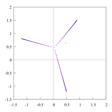
Let

$$f(z)=1/\bigl{(}(z-a_{1})(z-a_{2})(z-a_{3})\bigr{)}^{1/3},$$ (37)

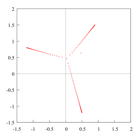
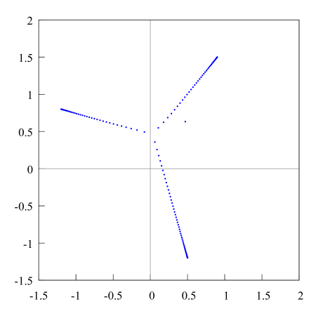
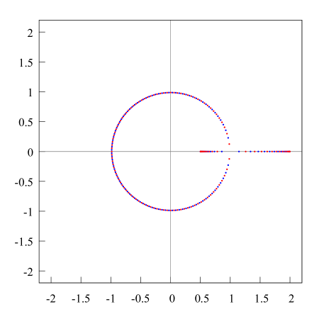
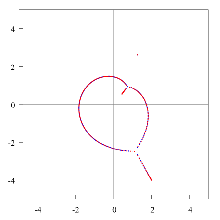
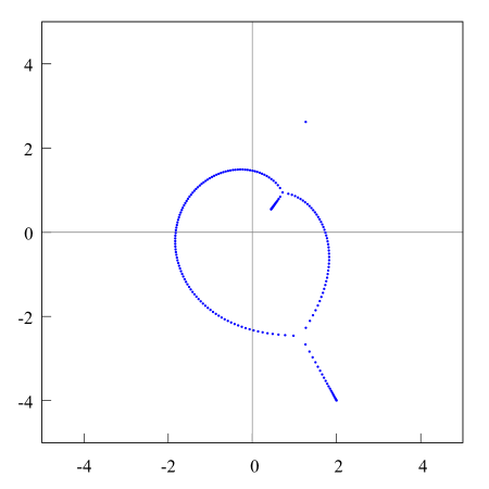
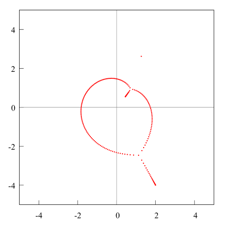
where $a_{1}=-1.2+0.8i$, $a_{2}=0.9+1.5i$, $a_{3}=0.5-1.2i$. On Figure 1, the zeros (blue points) and the poles (red points) of the PA $[130/130]_{f}$ of $f$ at infinity are plotted. On Fig. 3 and Fig. 2 the zeros (blue points) and the poles (red points) of PA $[130/130]_{f}$ are plotted separately. Clearly, numerical zero-pole distribution is in good agreement with the statements of Stahl Theorem. But there is a spurious zero-pole pair, which does not correspond to any singularity of the given function (37). The behavior of this pair as $n\to\infty$ is not governed by Stahl Theorem, since this theorem is dealing with a weak-star limit zero-pole distribution of PA. This kind of behavior was discovered by Nuttall [53] in 1986 via a suitable modification of Liouville–Steklov method (see also [44]). However, Nuttall’s result was found only after Stahl Theorem was proved. To be more precise, Nuttall used the existence of Stahl’s $S$-curve for the function (37).

Namely, Nuttall first proved that Padé polynomials of order $n$ and the remainder function for the function (37) both solve a linear homogeneous differential equation of second order, with polynomial coefficients of fixed degrees. These polynomials have some accessory parameters depending on $n$. Subsequently, Nuttall proved that Stahl’s $S$-curve is the limit, as $n\to\infty$, of the Stokes lines for these differential equations, that depend on $n$. Finally, in [53] Nuttall proved that there may exist only one spurious zero-pole pair of PA to the function (37), since the two-sheeted Stahl’s Riemann surface $\mathfrak{R}_{2}$, associated with the function (37), is of genus $g=1$. Nuttall proved that if the zero and the pole of a spurious zero-pole pair are close to one another, then they actually cancel each other, as $n\to\infty$. But if, for each $n\in\mathbb{N}$, they do not coincide with each other, then they are everywhere dense on the Riemann sphere, as $n\to\infty$. Describing the behavior of the spurious zero-pole pairs might require solving the so-called “Jacobi inversion problem” (see [63]), that is an equation with an Abelian integral of first kind on the left and some expression that is linear in $n$ on the right. Thus, as $n\to\infty$, such pairs form some type of “winding of the torus”, which is everywhere dense on that torus, that is, dense on the Stahl’s two-sheeted Riemann surface $\mathfrak{R}_{2}$ of genus $g=1$. The fact that the zero and the pole in some sense cancel each other in such a zero-pole pair, as $n\to\infty$, is in full agreement with the pure numerical results that were obtained by M. Froissart [20], see also [11, Chapter 2, § 2.2] and [74].

4.1.2. The case of a function with several branch points, Chebotarev–Stahl’s $S$-curve and Stahl limit zero-pole distribution theorem

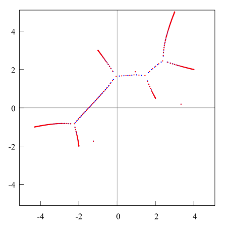
Let

$$f(z)=1/\bigl{(}(z-a_{1})\cdot\dotso\cdot(z-a_{6})\bigr{)}^{1/6},$$ (38)

where $a_{1}=4.3+i$, $a_{2}=2+0.5i$, $a_{3}=2+2i$, $a_{4}=1-3i$, $a_{5}=4+2i$, $a_{6}=3+5i$. On Fig. 4 are plotted zeros (blue points) and poles (red points) of the PA $[103/103]_{f}$, taken at the infinity point $z=\infty$ to the function $f$ given by (38). Clearly, numerical zero-pole distribution is in good agreement with the statements of Stahl Theorem. But there are spurious zero-pole pairs, which do not correspond to singularities of the given function (38). The behavior of this pair, as $n\to\infty$, is not governed by Stahl Theorem, since it is about weak-star limit zero-pole distribution of PA. This behavior was discovered by A. Martinez-Finkelshtein, E. A. Rakhmanov, and S. P. Suetin [44] in 2012 via a suitable modification of Liouville–Steklov method (cf. [53]). This result was obtained on the base of Stahl Theorem. More precisely: the authors of [44] used the basic fact about the existence of Stahl’s $S$-curve for the function (38). Namely, first they proved that Padé polynomials of order $n$, as well as the remainder function for the function (38) solve a linear homogeneous differential equation of second order with polynomial coefficients of fixed degrees. These polynomials have some accessory parameters depending on $n$. Second, they showed that Stahl’s $S$-curve is the limit, as $n\to\infty$, of the Stokes lines for these differential equations, depending on $n$. Ultimately, the authors concluded that no more than four spurious zero-pole pairs of PA of the function (38) may exist. The reason is that the Stahl’s two-sheeted Riemann surface $\mathfrak{R}_{2}$, which corresponds to the function (38), is of genus $g=4$. It was proved that the zero and the pole in each spurious zero-pole pair are close to each other and they cancel each other, as $n\to\infty$. However, in the “generic case”, if they do not coincide with each other for each $n\in\mathbb{N}$, then they are everywhere dense on the Riemann sphere, as $n\to\infty$. Describing the behavior of the spurious zero-pole pairs might require solving a system of equations with some Abelian integrals of first kind on the left side and some expressions, which are linear in $n$, on the right side. The fact that the zero and pole in some sense cancel each other in such a zero-pole pair as $n\to\infty$ is in full agreement with the pure numerical results obtained by M. Froissart [20], see also [11, Chapter 2, § 2.2] and [74].

4.2. Some numerical examples for two-point Padé approximants

Let

$$f(z)=\left(\frac{z-a_{1}}{z-a_{2}}\right)^{1/4},$$ (39)

where $a_{1}=0.9-1.1i$, $a_{2}=0.1+0.2i$. Suppose that two “different” germs are taken, $f_{0}$ and $f_{\infty}$ of the function (39) at the point $z=0$ and at the infinity point $z=\infty$, respectively. Here, “different” means that to obtain the germ $f_{\infty}\in\mathscr{H}(\infty)$ by the analytic continuation of the germ $f_{0}\in\mathscr{H}(0)$, we should go along a path that encircles exactly one time one of the branch points ($a_{1}$ or $a_{2}$).

On Fig. 6 are plotted the zeros and poles of two-point PA $[199/199]_{f_{0},f_{\infty}}$ to the function (39). On Fig. 7 and Fig. 8 are plotted separately the zeros (blue points) and poles (red points) of the two-point PA $[199/199]_{f_{0},f_{\infty}}$ for the function (39). This numerical zero-pole distribution of two-point PA $[199/199]_{f_{0},f_{\infty}}$ is in full agreement with Buslaev’s limit zero-pole distribution theorem [14]. Similarly to the function (37) and classical PA, the two-sheeted Riemann surface, associated with the function (39) and the two-point PA, is of genus $g=1$. Therefore, similarly to the case of classical PA, there is a single zero-pole pair of spurious character. The behavior of this pair, as $n\to\infty$, cannot be described by Buslaev Theorem, since the theorem is only about weak-star convergence of two-point PA.

The description of this behavior for the special function (39) and under the condition of a “generic case”, imposed on the branch points $a_{1}$ and $a_{2}$, was done by Komlov and Suetin in [33]. Under this condition, in [33] was derived a formula of the strong asymptotics for two-point PA. The method producing this formula is similar to Nuttall’s method for classical PA, see [53] and [44]. In [33], it was proved first that for each $n\in\mathbb{N}$ the two-point Padé polynomials and the corresponding remainder function solve the homogeneous linear differential equation of second order with polynomial coefficients of fixed degrees, but depending on $n$. After that, it was proved that Buslaev’s $S$-curve forms the limit, as $n\to\infty$, of the Stokes lines for these differential equations. Finally, a formula of the strong asymptotics for the two-point PA was found via the asymptotic Liouville–Steklov method.

4.3. Some numerical examples for Hermite-Padé polynomials

Now we are ready to make some short description of the obtained numerical results for the HP of the collection of three functions $[1,f_{1},f_{2}]$.

4.3.1. Parameter $a=-0.1$: logarithmic functions, Fig. 9–Fig. 10, square root functions, Fig. 11–Fig. 12

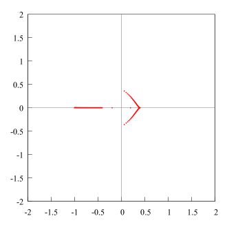
At first we set $a=-0.1$ (and keep $n=200$). Clearly, that value of $a$ is out of the range of $(0,1)$. But in that case all three pairs $f_{1},f_{2}$, $g_{1},g_{2}$ and $h_{1},h_{2}$ form Angelesco systems, since $E_{1},E_{2}\subset\mathbb{R}$ and $E_{1}\cap E_{2}=\varnothing$. On Fig. 9, Fig. 10, Fig. 11, and Fig. 12 are plotted the zeros of HP polynomials $Q_{200,j}$ and $P_{200,j}$, $j=0,1,2$. The numerical distribution of the zeros of the HP polynomials are similar in both cases, and it does not depend on the different type of branching of the functions $f_{1},f_{2}$ and $g_{1},g_{2}$ at the points $z=\pm 1,\pm a$. The reason is as follows. All these numerical results are in a full agreement with the general theory of limit zero distribution (LZD) for HP polynomials in the Angelesco case (see [21], [26], [4]; in these papers the case of type II HP polynomials was considered, but it is well known that in the Angelesco case there is a direct connection between LZD of type I and type II HP polynomials). Since the size of the supports of Markov-type functions $f_{1}$ and $f_{2}$ (and $g_{1}$, $g_{2}$ as well) are equal, the phenomena of the so-called “pushing of the charge” is absent in the case when $a=-0.1$. It is also in full agreement with the general theory (see [30], [1], [21]). From Fig. 9 and Fig. 10 follows, that the zeros of HP polynomials $Q_{200,1}$ and $Q_{200,2}$ (and $P_{200,1}$, $P_{200,2}$ as well) are located on the segments $E_{1}$ and $E_{2}$, respectively. But the zeros of $Q_{200,0}$ (and $P_{200,0}$ respectively) are located on the imaginary axis. Thus, in some sense, the zeros of $Q_{200,0}$ “intend to separate” the zeros of $Q_{200,1}$ and $Q_{200,2}$ from each other. Again, this result is in good agreement with the well known LZD of type I HP polynomials in the Angelesco case (see, e.g. [54]). To finish the analysis of the case $a=-0.1$, we emphasize that in this case all numerical results are in good agreement with the general theory of HP polynomials. Thus it is reasonable to consider all numerical results for $a=0.2;0.4;0.625;0.73;0.8$ as to be trustable.

4.3.2. Parameter $a=0.2$: logarithmic functions, Fig. 13–Fig. 16

Now let $a=0.2$. For this value of the parameter $a$, the intersection of the two segments $E_{1}=[-1,a]$ and $E_{2}=[-a,1]$ equals $E_{1}\cap E_{2}=\Delta=[-a,a]\not=\varnothing$, that is, $\Delta$ is small, but nonempty real segment.

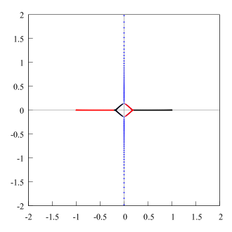
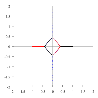
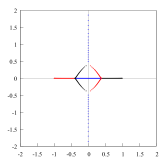
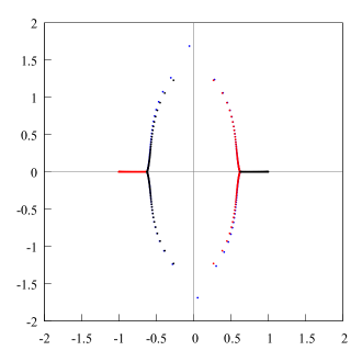
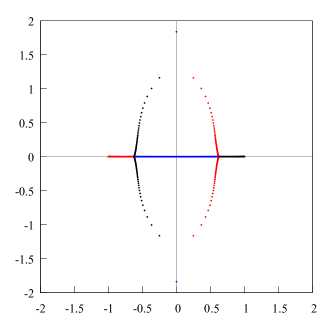
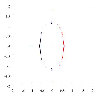
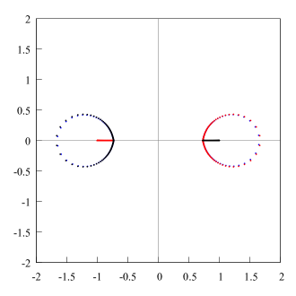
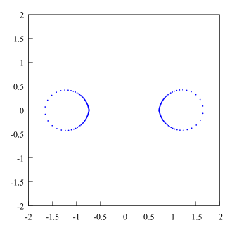
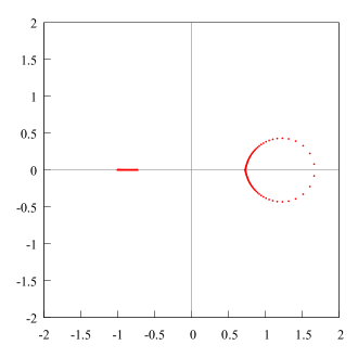
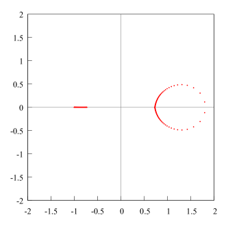
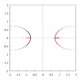
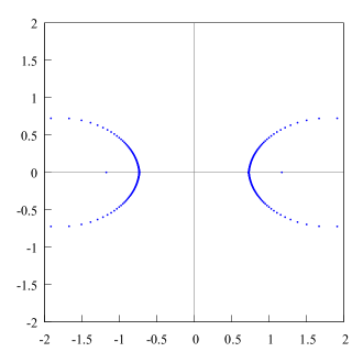
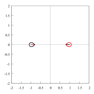
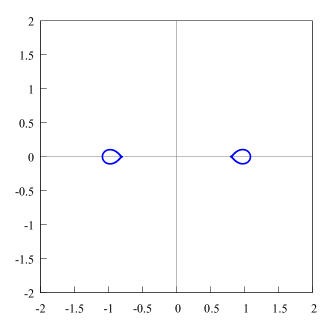
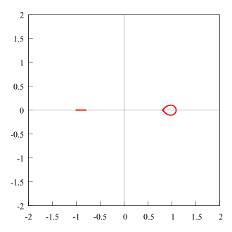
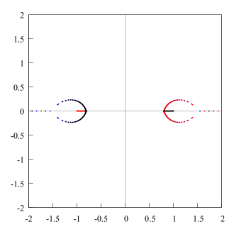
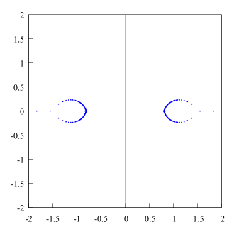
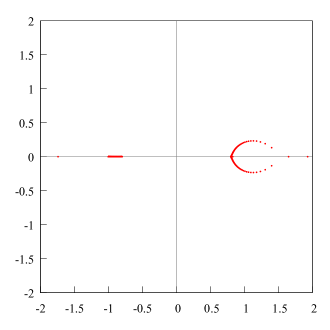
In all three cases, Case 1, Case 2, and Case 3, the numerical zero distribution (NZD) of HP $Q_{200,j}(z;f_{1},f_{2})$, $P_{200,j}(z;g_{1},g_{2})$, and $U_{200,j}(z;h_{1},h_{2})$ for $j=1,2$ are similar to each other. Thus, here we only discuss the NZD for HP $Q_{200,1}$ and $Q_{200,2}$ (these zeros are plotted by red and black points respectively, see Fig. 15 and Fig. 16). Notice that zeros of $Q_{200,1}$ and $Q_{200,2}$ are symmetric to each other, with respect to the imaginary axis. Thus, it is enough to only consider the NZD for HP $Q_{200,2}$ (these zeros are plotted in black; see Fig. 16).

For this value of the parameter $a$, the essential part of zeros of HP $Q_{200,2}$ are located not on the real line, but somewhere in the complex plane. Evidently, this set is symmetric with respect to the real axis, since we consider Markov-type functions. Due to the general conjectures (see [52], [69]), that are based on the seminal paper by Gonchar and Rakhmanov [21] about LZD of pure Angelesco system of Markov-type functions, the LZD for HP $Q_{n,2}$, as $n\to\infty$, should be described via an equilibrium measure, say $\lambda_{2}$, that is associated with some special $\max$-$\min$ extremal theoretical potential problem. From Fig. 16 (see also Fig. 15) it follows immediately, that in the case $a=0.2$ the support of the measure $\lambda_{2}$ should be a disconnected set. The same is true for the equilibrium measure $\lambda_{1}$, that is associated with LZD for HP $Q_{n,1}$. The union $S_{1}(f_{1},f_{2})\cup S_{2}(f_{1},f_{2})$ of two compact sets $S_{1}(f_{1},f_{2})=\operatorname{supp}\lambda_{1}$ and $S_{2}(f_{1},f_{2})=\operatorname{supp}\lambda_{2}$ form some type of lenses. From the general approach, based on the paper by Gonchar and Rakhmanov [24] about “$1/9$-conjecture”, it follows, that the compact sets $S_{1}(f_{1},f_{2})$ and $S_{2}(f_{1},f_{2})$ should be a weighted $S$-curve (see also [59]). Notice, that in both cases the open sets $\overline{\mathbb{C}}\setminus S_{1}(f_{1},f_{2})$ and $\overline{\mathbb{C}}\setminus S_{2}(f_{1},f_{2})$ are also domains (see Fig. 15 and Fig. 16 respectively).

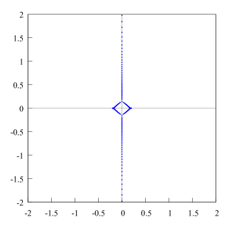
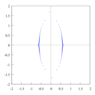
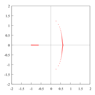
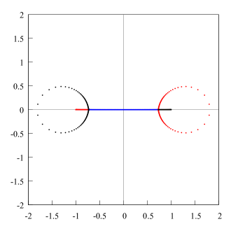
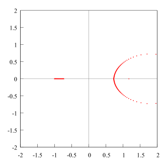
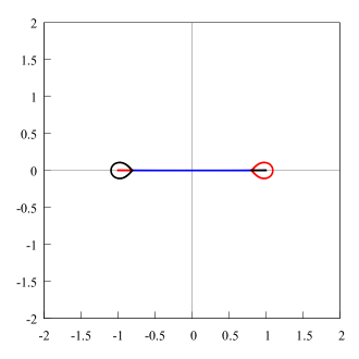
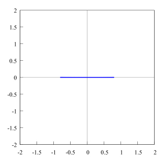
It follows from Fig. 14, that the LZD for HP $Q_{n,0}$ should be quite different from the LZD for HP $Q_{n,1}$ and $Q_{n,2}$. The reason is as follows. This LZD should be described by an extremal $\max$-$\min$ theoretical potential problem of different type than before. In part, the support $S_{0}(f_{1},f_{2})$ of the equilibrium measure $\lambda_{0}$, associated with this extremal theoretical potential problem, should be a continuum, i.e. a connected compact set. But now, the open set $\overline{\mathbb{C}}\setminus S_{0}(f_{1},f_{2})$ is not a domain, since it consists of three domains. The compact set $S_{0}(f_{1},f_{2})$ should also be a weighted $S$-curve, but of some other nature than the compact sets $S_{1}(f_{1},f_{2})$ and $S_{2}(f_{1},f_{2})$. In particular, there should be three Chebotarev’s points on the compact set $S_{0}(f_{1},f_{2})$, i.e. the points of zero density of the equilibrium measure $\lambda_{0}$. One of these points is located on the upper half plane, the other point is located on lower half plane, and the third Chebotarev’s point coincides with the infinity point. Notice, that similarly to the case when $a=-0.1$, now the $S$-curve $S_{0}(f_{1},f_{2})$ separates the $S$-curves $S_{1}(f_{1},f_{2})$ and $S_{2}(f_{1},f_{2})$ from each other. It might be conjectured that the pair $S_{(}f_{1},f_{2}),S_{2}(f_{1},f_{2})$ forms some kind of weighted Nuttall’s condenser (see [61]).

4.3.3. Parameter $a=0.2$: square root functions, Fig. 17–Fig. 20, and cubic root functions, Fig. 21–Fig. 24

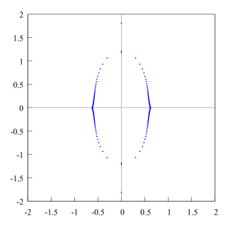
The NZD of HP $P_{200,1}$ and $P_{200,2}$ for the square root functions, given by (5), (6), and NZD of HP polynomials $U_{200,1}$ and $U_{200,2}$ for the cubic root functions, given by (7), (8), are similar to the NZD of HP $Q_{200,1}$ and $Q_{200,2}$, for the pair of logarithmic functions given by (3), (4), respectively (see Fig. 19, Fig. 20, Fig. 23, and Fig. 24). It is also valid for the HP $U_{200,0}$, i.e. this NZD is similar to the NZD of HP $Q_{200,0}$ for the given logarithmic functions. Therefore, we do not discuss specially the NZD of HP $P_{200,1}$, $P_{200,2}$, $U_{200,1}$, $U_{200,2}$, and $U_{200,0}$. Notice, that there is a pair of spurious zeros of the HP $U_{200,0}$ (see Fig. 22). From that numerical fact follows, that the genus of the associated three-sheeted Riemann surface $\mathfrak{R}_{3}$ should be equal to $2$ (cf. [54], [2]).

4.3.4. Parameter $a=0.2$: square root functions, NZD of $P_{200,0}$, Fig. 18

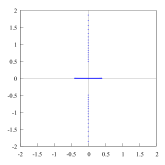
The NZD of HP polynomials $P_{200,0}$ is quite different from NZD of HP $Q_{200,0}$ (see Fig. 14) and $U_{200,0}$ (see Fig. 22). In fact, from the numerical results follows, that the associated $S$-curve $S_{0}(g_{1},g_{2})$ should consist of two segments, and the open set $\overline{\mathbb{C}}\setminus S_{0}(g_{1},g_{2})$ should be a domain. In that case, the compact set $S_{0}(g_{1},g_{2})$ separates distinctly the other $S$-curves $S_{1}(g_{1},g_{2})$ and $S_{2}(g_{1},g_{2})$ from each other.

4.3.5. Parameter $a=0.4$: logarithmic functions, Fig. 25–Fig. 28, square root functions, Fig. 29–Fig. 32, cubic root functions, Fig. 33–Fig. 36; parameter $a=0.625$: logarithmic functions, Fig. 37–Fig. 40, square root functions, Fig. 41–Fig. 44, cubic root functions, Fig. 45–Fig. 48

For these two values of the parameter $a$ all the NZD of HP $Q_{200,j}$, $P_{200,j}$, $U_{200,j}$, $j=0,1,2$, are similar to the case when $a=0.2$. The observed difference does not change the principal structure of the associated $S$-curves and is the following. The lenses, that appeared for parameter $a=0.2$, become larger and larger when $a$ changes from $0.2$ to the values $a=0.4$ and $a=0.625$. The positions of all four vertices of the lenses are not fixed, but depend on the value of the parameter $a$. When the parameter $a$ increases from $a=0.2$ to $a=0.4$ and after that to $a=0.625$, the two real vertices move from the inside of the segment $[-1,1]$ towards to the end points $\pm 1$. In addition, the two pure imaginary vertices move along simultaneously from the imaginary axis to the infinity point, where they meet each other, under some critical value of the parameter $a^{*}\in(0.625,0.73)$ (see the next Fig. 49–Fig. 72; the statement on the existence of the critical value $a^{*}$ is based only on numerical results and should be considered as a conjecture). As usually, the NZD of HP $P_{200,0}$ corresponds to the whole segment $[-a,a]$. Hence, the blue segment on Fig. 18, Fig. 30, and Fig. 42 becomes wider and wider as the parameter $a$ increases form $a=0.2$ to $a=0.625$.

4.3.6. Parameter $a=0.73$: logarithmic functions, Fig. 49–Fig. 52, square root functions, Fig. 53–Fig. 56, cubic root functions, Fig. 57–Fig. 60; parameter $a=0.8$: logarithmic functions, Fig. 61–Fig. 64, square root functions, Fig. 65–Fig. 68, cubic root functions, Fig. 69–Fig. 72

After $a>a^{*}$, where $a^{*}$ is the critical value of the parameter $a$ described above, the NZD of HP $Q_{200,j}$, $P_{200,j}$, $U_{200,j}$, $j=0,1,2$, dramatically changes. Namely, the complements $\overline{\mathbb{C}}\setminus S_{1}$ and $\overline{\mathbb{C}}\setminus S_{2}$ of the $S$-curves $S_{1}$ and $S_{2}$ are now disconnected open sets, instead of domains, as they were when $a<a^{*}$. Plotted on a single picture, all three numerical sets $S_{1},S_{2},S_{3}$, that consist of red, black, and blue points, respectively, form in these three cases three quite different structures. For instance, when the parameter $a$ equals $0.8$, in Case 1 the associated $S$-curve $S_{0}(f_{1},f_{2})$ becomes a disconnected compact set, namely, $S_{0}(f_{1},f_{2})$ consists of two continua (see Fig. 62). In Case 2, we have $S_{0}(g_{1},g_{2})=[-a,a]$ (see Fig. 66), and finally, in Case 3 the $S$-curve $S_{0}(h_{1},h_{2})$ is a continua that contains the infinity point (see Fig. 70). In the last case, $S_{0}(h_{1},h_{2})$ contains two Chebotarev’s points that are the points of zero density for the corresponding equilibrium measure $\lambda_{0}$ with $\operatorname{supp}\lambda_{0}=S_{0}(h_{1},h_{2})$.

Figure 1. Zeros and poles of the diagonal Padé approximant $[130/130]_{f}$ of the function $f(z)=1/((z-(-1.2+0.8i))(z-(0.9+1.5i))(z-(0.5-1.2i)))^{1/3}$, distributed accordingly to the electrostatical model by E. A. Rakhmanov [59]. There is a Froissart doublet (spurious zero-pole pair) when $n=130$ (see also Fig. 2 and Fig. 3). Since the genus of the Riemann surface is $1$, there might be at most one Froissart doublet. In full compliance with the Rakhmanov model [59], the Froissart doublet “attracts” the Stahl $S$-compact $S_{130}$.

Figure 2. The poles of the Padé approximant $[130/130]_{f}$ approximate a Chebotarev point $v_{130}$ for the $S$-compact $S_{130}$ (see [59]). The Chebotarev point is at $(0.029,0.466)$. When $n\to\infty$ we have that $v_{n}\to v$ is a classical Chebotarev point. There is one spurious pole of the Padé approximant $[130/130]_{f}$, it is accompanied by a spurious zero of the Padé approximant $[130/130]_{f}$ (see Fig. 3). The spurious zero-pole is at $(0.469,0.633)$.

Figure 3. The Chebotarev point should not be approximated by zeros of the Padé approximant $[130/130]_{f}$ of the function (37). Evidently, the Cheboratev point does not exist on the picture. There is one spurious zero of the Padé approximant $[130/130]_{f}$, it is accompanied by a spurious pole of the Padé approximant $[130/130]_{f}$ (see Fig. 2).

Figure 4. Zeros and poles of the diagonal Padé approximant $[103/103]_{f}$ of the function $f(z)=1/((z+(4.3+1.0i))(z-(2.0+0.5i))(z+(2.0+2.0i))(z+(1.0-3.0i))(z-(4.0+2.0i))(z-(3.0+5.0i)))^{1/6}$. These zeros and poles are distributed in a plane, under fixed $n=103$, accordingly to the electrostatical model by Rakhmanov [59]. Since the genus of the Riemann surface is $4$, for each $n$ there might be no more than 4 Froissart doublets. Here are observed 3 Froissart doublets. In full compliance with the Rakhmanov model, the Froissart doublets “attract” the Stahl $S$-compact $S_{103}$. In general, the zeros and poles of the diagonal Padé approximants $[n/n]_{f}$ are distributed as $n\to\infty$ accordingly to Stahl Theorem [71].

Figure 5. Numerical zeros and poles distribution of two-point Padé approximants $[120/120]$ to the set of functions $\mathfrak{f}=\{f_{0},f_{\infty}\}$, where $f_{0}=((1-2z)(2-z))^{-1/2}$, $f_{\infty}=((2z-1)(z-2))^{-1/2}+1$. The germs $f_{0}$ and $f_{\infty}$ result in two different multivalued analytic functions. Thus, this is a generic case and by Buslaev Theorem the associated $S$-curve partitions the Riemann sphere into two domains.

Figure 6. Numerical zeros and poles distribution of two-point Padé approximants $[199/199]$ to the function $f(z)=((z-a_{1})/(z-a_{2}))^{1/4}$, where $a_{1}=0.9-1.1i$ and $a_{2}=0.1+0.2i$. Here are selected two “different branches” of the function $f$, namely, $f_{0}=((z-a_{1})/(z-a_{2}))^{1/4}$ and $f_{\infty}=-((z-a_{1})/(z-a_{2}))^{1/4}$. Almost all zeros (blue points) and poles (red points) approximate numerically Buslaev’s compact set. But there is a spurious zero-pole pair that moves as $n\to\infty$ under the order of equation from [33].

Figure 7. Numerical zeros distribution of two-point Padé approximants $[199/199]$ to the function $f(z)=((z-a_{1})/(z-a_{2}))^{1/4}$, where $a_{1}=0.9-1.1i$ and $a_{2}=0.1+0.2i$. Here are selected two “different branches” of the function $f$, namely, $f_{0}=((z-a_{1})/(z-a_{2}))^{1/4}$ and $f_{\infty}=-((z-a_{1})/(z-a_{2}))^{1/4}$. Almost all zeros (blue points) approximate numerically Buslaev’s compact set. But there is a spurious zero-pole pair that moves as $n\to\infty$ under the order of equation from [33].

Figure 8. Numerical poles distribution of two-point Padé approximants $[199/199]$ to the function $f(z)=((z-a_{1})/(z-a_{2}))^{1/4}$, where $a_{1}=0.9-1.1i$ and $a_{2}=0.1+0.2i$. Here are selected two “different branches” of the function $f$, namely, $f_{0}=((z-a_{1})/(z-a_{2}))^{1/4}$ and $f_{\infty}=-((z-a_{1})/(z-a_{2}))^{1/4}$. Almost all poles (red points) approximate numerically Buslaev’s compact set. But there is a spurious zero-pole pair that moves as $n\to\infty$ under the order of equation from [33].

Figure 9. Numerical distribution of zeros of type I Hermite–Padé polynomials $Q_{200,0}$ (blue points), $Q_{200,1}$ (red points), $Q_{200,2}$ (black points), for the collection of functions $[1,f_{1},f_{2}]$, where $f_{1}=\log((0.1+1/z)/(1+1/z))$, $f_{2}=\log((0.1-1/z)/(1-1/z))$.

Figure 10. Numerical distribution of zeros of type I Hermite–Padé polynomials $Q_{200,0}$ (blue points) for the collection of functions $[1,f_{1},f_{2}]$, where $f_{1}=\log((0.1+1/z)/(1+1/z))$, $f_{2}=\log((0.1-1/z)/(1-1/z))$.

Figure 11. Numerical distribution of zeros of type I Hermite–Padé polynomials $P_{200,0}$ (blue points), $P_{200,1}$ (red points), $P_{200,2}$ (black points), for the collection of functions $[1,g_{1},g_{2}]$, where $g_{1}=((0.1+1/z)/(1+1/z))^{1/2}$, $g_{2}=((0.1-1/z)/(1-1/z))^{1/2}$.

Figure 12. Numerical distribution of zeros of type I Hermite–Padé polynomials $P_{200,0}$ (blue points) for the collection of functions $[1,g_{1},g_{2}]$, where $g_{1}=((0.1+1/z)/(1+1/z))^{1/2}$, $g_{2}=((0.1-1/z)/(1-1/z))^{1/2}$.

Figure 13. Numerical distribution of zeros of type I Hermite–Padé polynomials $Q_{200,0}$ (blue points), $Q_{200,1}$ (red points), $Q_{200,2}$ (black points), for the collection of functions $[1,f_{1},f_{2}]$, where $f_{1}=\log((0.2-1/z)/(1+1/z))$, $f_{2}=\log((0.2+1/z)/(1-1/z))$.

Figure 14. Numerical distribution of zeros of type I Hermite–Padé polynomials $Q_{200,0}$ (blue points) for the collection of functions $[1,f_{1},f_{2}]$, where $f_{1}=\log((0.2-1/z)/(1+1/z))$, $f_{2}=\log((0.2+1/z)/(1-1/z))$.

Figure 15. Numerical distribution of zeros of type I Hermite–Padé polynomials $Q_{200,1}$ (red points) for the collection of functions $[1,f_{1},f_{2}]$, where $f_{1}=\log((0.2-1/z)/(1+1/z))$, $f_{2}=\log((0.2+1/z)/(1-1/z))$.

Figure 16. Numerical distribution of zeros of type I Hermite–Padé polynomials $Q_{200,2}$ (black points) for the collection of functions $[1,f_{1},f_{2}]$, where $f_{1}=\log((0.2-1/z)/(1+1/z))$, $f_{2}=\log((0.2+1/z)/(1-1/z))$.

Figure 17. Numerical distribution of zeros of type I Hermite–Padé polynomials $P_{200,0}$ (blue points), $P_{200,1}$ (red points), $P_{200,2}$ (black points), for the collection of functions $[1,g_{1},g_{2}]$, where $g_{1}=((0.2-1/z)/(1+1/z))^{1/2}$, $g_{2}=((0.2+1/z)/(1-1/z))^{1/2}$.

Figure 18. Numerical distribution of zeros of type I Hermite–Padé polynomials $P_{200,0}$ (blue points) for the collection of functions $[1,g_{1},g_{2}]$, where $g_{1}=((0.2-1/z)/(1+1/z))^{1/2}$, $g_{2}=((0.2+1/z)/(1-1/z))^{1/2}$.

Figure 19. Numerical distribution of zeros of type I Hermite–Padé polynomials $P_{200,1}$ (red points) for the collection of functions $[1,g_{1},g_{2}]$, where $g_{1}=((0.2-1/z)/(1+1/z))^{1/2}$, $g_{2}=((0.2+1/z)/(1-1/z))^{1/2}$.

Figure 20. Numerical distribution of zeros of type I Hermite–Padé polynomials $P_{200,2}$ (black points) for the collection of functions $[1,g_{1},g_{2}]$, where $g_{1}=((0.2-1/z)/(1+1/z))^{1/2}$, $g_{2}=((0.2+1/z)/(1-1/z))^{1/2}$.

Figure 21. Numerical distribution of zeros of type I Hermite–Padé polynomials $U_{200,0}$ (blue points), $U_{200,1}$ (red points), $U_{200,2}$ (black points), for the collection of functions $[1,h_{1},h_{2}]$, where $h_{1}=((0.2-1/z)/(1+1/z))^{1/3}$, $h_{2}=((0.2+1/z)/(1-1/z))^{1/3}$.

Figure 22. Numerical distribution of zeros of type I Hermite–Padé polynomials $U_{200,0}$ (blue points) for the collection of functions $[1,h_{1},h_{2}]$, where $h_{1}=((0.2-1/z)/(1+1/z))^{1/3}$, $h_{2}=((0.2+1/z)/(1-1/z))^{1/3}$.

Figure 23. Numerical distribution of zeros of type I Hermite–Padé polynomials $U_{200,1}$ (red points) for the collection of functions $[1,h_{1},h_{2}]$, where $h_{1}=((0.2-1/z)/(1+1/z))^{1/3}$, $h_{2}=((0.2+1/z)/(1-1/z))^{1/3}$.

Figure 24. Numerical distribution of zeros of type I Hermite–Padé polynomials $U_{200,2}$ (black points) for the collection of functions $[1,h_{1},h_{2}]$, where $h_{1}=((0.2-1/z)/(1+1/z))^{1/3}$, $h_{2}=((0.2+1/z)/(1-1/z))^{1/3}$.

Figure 25. Numerical distribution of zeros of type I Hermite–Padé polynomials $Q_{200,0}$ (blue points), $Q_{200,1}$ (red points), $Q_{200,2}$ (black points), for the collection of functions $[1,f_{1},f_{2}]$, where $f_{1}=\log((0.4-1/z)/(1+1/z))$, $f_{2}=\log((0.4+1/z)/(1-1/z))$.

Figure 26. Numerical distribution of zeros of type I Hermite–Padé polynomials $Q_{200,0}$ (blue points) for the collection of functions $[1,f_{1},f_{2}]$, where $f_{1}=\log((0.4-1/z)/(1+1/z))$, $f_{2}=\log((0.4+1/z)/(1-1/z))$.

Figure 27. Numerical distribution of zeros of type I Hermite–Padé polynomials $Q_{200,1}$ (red points) for the collection of functions $[1,f_{1},f_{2}]$, where $f_{1}=\log((0.4-1/z)/(1+1/z))$, $f_{2}=\log((0.4+1/z)/(1-1/z))$.

Figure 28. Numerical distribution of zeros of type I Hermite–Padé polynomials $Q_{200,2}$ (black points) for the collection of functions $[1,f_{1},f_{2}]$, where $f_{1}=\log((0.4-1/z)/(1+1/z))$, $f_{2}=\log((0.4+1/z)/(1-1/z))$.

Figure 29. Numerical distribution of zeros of type I Hermite–Padé polynomials $P_{200,0}$ (blue points), $P_{200,1}$ (red points), $P_{200,2}$ (black points), for the collection of functions $[1,g_{1},g_{2}]$, where $g_{1}=((0.4-1/z)/(1+1/z))^{1/2}$, $g_{2}=((0.4+1/z)/(1-1/z))^{1/2}$.

Figure 30. Numerical distribution of zeros of type I Hermite–Padé polynomials $P_{200,0}$ (blue points) for the collection of functions $[1,g_{1},g_{2}]$, where $g_{1}=((0.4-1/z)/(1+1/z))^{1/2}$, $g_{2}=((0.4+1/z)/(1-1/z))^{1/2}$.

Figure 31. Numerical distribution of zeros of type I Hermite–Padé polynomials $P_{200,1}$ (red points) for the collection of functions $[1,g_{1},g_{2}]$, where $g_{1}=((0.4-1/z)/(1+1/z))^{1/2}$, $g_{2}=((0.4+1/z)/(1-1/z))^{1/2}$.

Figure 32. Numerical distribution of zeros of type I Hermite–Padé polynomials $P_{200,2}$ (black points) for the collection of functions $[1,g_{1},g_{2}]$, where $g_{1}=((0.4-1/z)/(1+1/z))^{1/2}$, $g_{2}=((0.4+1/z)/(1-1/z))^{1/2}$.

Figure 33. Numerical distribution of zeros of type I Hermite–Padé polynomials $U_{200,0}$ (blue points), $U_{200,1}$ (red points), $U_{200,2}$ (black points), for the collection of functions $[1,h_{1},h_{2}]$, where $h_{1}=((0.4-1/z)/(1+1/z))^{1/3}$, $h_{2}=((0.4+1/z)/(1-1/z))^{1/3}$.

Figure 34. Numerical distribution of zeros of type I Hermite–Padé polynomials $Q_{200,0}$ (blue points) for the collection of functions $[1,h_{1},h_{2}]$, where $h_{1}=((0.4-1/z)/(1+1/z))^{1/3}$, $h_{2}=((0.4+1/z)/(1-1/z))^{1/3}$.

Figure 35. Numerical distribution of zeros of type I Hermite–Padé polynomials $U_{200,1}$ (red points) for the collection of functions $[1,h_{1},h_{2}]$, where $h_{1}=((0.4-1/z)/(1+1/z))^{1/3}$, $h_{2}=((0.4+1/z)/(1-1/z))^{1/3}$.

Figure 36. Numerical distribution of zeros of type I Hermite–Padé polynomials $U_{200,2}$ (black points) for the collection of functions $[1,h_{1},h_{2}]$, where $h_{1}=((0.4-1/z)/(1+1/z))^{1/3}$, $h_{2}=((0.4+1/z)/(1-1/z))^{1/3}$.

Figure 37. Numerical distribution of zeros of type I Hermite–Padé polynomials $Q_{200,0}$ (blue points), $Q_{200,1}$ (red points), $Q_{200,2}$ (black points), for the collection of functions $[1,f_{1},f_{2}]$, where $f_{1}=\log((0.625-1/z)/(1+1/z))$, $f_{2}=\log((0.625+1/z)/(1-1/z))$.

Figure 38. Numerical distribution of zeros of type I Hermite–Padé polynomials $Q_{200,0}$ (blue points) for the collection of functions $[1,f_{1},f_{2}]$, where $f_{1}=\log((0.625-1/z)/(1+1/z))$, $f_{2}=\log((0.625+1/z)/(1-1/z))$.

Figure 39. Numerical distribution of zeros of type I Hermite–Padé polynomials $Q_{200,1}$ (red points) for the collection of functions $[1,f_{1},f_{2}]$, where $f_{1}=\log((0.625-1/z)/(1+1/z))$, $f_{2}=\log((0.625+1/z)/(1-1/z))$.

Figure 40. Numerical distribution of zeros of type I Hermite–Padé polynomials $Q_{200,2}$ (black points) for the collection of functions $[1,f_{1},f_{2}]$, where $f_{1}=\log((0.625-1/z)/(1+1/z))$, $f_{2}=\log((0.625+1/z)/(1-1/z))$.

Figure 41. Numerical distribution of zeros of type I Hermite–Padé polynomials $P_{200,0}$ (blue points), $P_{200,1}$ (red points), $P_{200,2}$ (black points), for the collection of functions $[1,g_{1},g_{2}]$, where $g_{1}=((0.625-1/z)/(1+1/z))^{1/2}$, $g_{2}=((0.625+1/z)/(1-1/z))^{1/2}$.

Figure 42. Numerical distribution of zeros of type I Hermite–Padé polynomials $P_{200,0}$ (blue points) for the collection of functions $[1,g_{1},g_{2}]$, where $g_{1}=((0.625-1/z)/(1+1/z))^{1/2}$, $g_{2}=((0.625+1/z)/(1-1/z))^{1/2}$.

Figure 43. Numerical distribution of zeros of type I Hermite–Padé polynomials $P_{200,1}$ (red points) for the collection of functions $[1,g_{1},g_{2}]$, where $g_{1}=((0.625-1/z)/(1+1/z))^{1/2}$, $g_{2}=((0.625+1/z)/(1-1/z))^{1/2}$.

Figure 44. Numerical distribution of zeros of type I Hermite–Padé polynomials $P_{200,2}$ (black points) for the collection of functions $[1,g_{1},g_{2}]$, where $g_{1}=((0.625-1/z)/(1+1/z))^{1/2}$, $g_{2}=((0.625+1/z)/(1-1/z))^{1/2}$.

Figure 45. Numerical distribution of zeros of type I Hermite–Padé polynomials $U_{200,0}$ (blue points), $U_{200,1}$ (red points), $U_{200,2}$ (black points), for the collection of functions $[1,h_{1},h_{2}]$, where $h_{1}=((0.625-1/z)/(1+1/z))^{1/3}$, $h_{2}=((0.625+1/z)/(1-1/z))^{1/3}$.

Figure 46. Numerical distribution of zeros of type I Hermite–Padé polynomials $U_{200,0}$ (blue points) for the collection of functions $[1,h_{1},h_{2}]$, where $h_{1}=((0.625-1/z)/(1+1/z))^{1/3}$, $h_{2}=((0.625+1/z)/(1-1/z))^{1/3}$.

Figure 47. Numerical distribution of zeros of type I Hermite–Padé polynomials $U_{200,1}$ (red points) for the collection of functions $[1,h_{1},h_{2}]$, where $h_{1}=((0.625-1/z)/(1+1/z))^{1/3}$, $h_{2}=((0.625+1/z)/(1-1/z))^{1/3}$.

Figure 48. Numerical distribution of zeros of type I Hermite–Padé polynomials $U_{200,2}$ (black points) for the collection of functions $[1,h_{1},h_{2}]$, where $h_{1}=((0.625-1/z)/(1+1/z))^{1/3}$, $h_{2}=((0.625+1/z)/(1-1/z))^{1/3}$.

Figure 49. Numerical distribution of zeros of type I Hermite–Padé polynomials $Q_{200,0}$ (blue points), $Q_{200,1}$ (red points), $Q_{200,2}$ (black points), for the collection of functions $[1,f_{1},f_{2}]$, where $f_{1}=\log((0.73-1/z)/(1+1/z))$, $f_{2}=\log((0.73+1/z)/(1-1/z))$.

Figure 50. Numerical distribution of zeros of type I Hermite–Padé polynomials $Q_{200,0}$ (blue points) for the collection of functions $[1,f_{1},f_{2}]$, where $f_{1}=\log((0.73-1/z)/(1+1/z))$, $f_{2}=\log((0.73+1/z)/(1-1/z))$.

Figure 51. Numerical distribution of zeros of type I Hermite–Padé polynomials $Q_{200,1}$ (red points) for the collection of functions $[1,f_{1},f_{2}]$, where $f_{1}=\log((0.73-1/z)/(1+1/z))$, $f_{2}=\log((0.73+1/z)/(1-1/z))$.

Figure 52. Numerical distribution of zeros of type I Hermite–Padé polynomials $Q_{200,2}$ (black points) for the collection of functions $[1,f_{1},f_{2}]$, where $f_{1}=\log((0.73-1/z)/(1+1/z))$, $f_{2}=\log((0.73+1/z)/(1-1/z))$.

Figure 53. Numerical distribution of zeros of type I Hermite–Padé polynomials $P_{200,0}$ (blue points), $P_{200,1}$ (red points), $P_{200,2}$ (black points), for the collection of functions $[1,g_{1},g_{2}]$, where $g_{1}=((0.73-1/z)/(1+1/z))^{1/2}$, $g_{2}=((0.73+1/z)/(1-1/z))^{1/2}$.

Figure 54. Numerical distribution of zeros of type I Hermite–Padé polynomials $P_{200,0}$ (blue points) for the collection of functions $[1,g_{1},g_{2}]$, where $g_{1}=((0.73-1/z)/(1+1/z))^{1/2}$, $g_{2}=((0.73+1/z)/(1-1/z))^{1/2}$.

Figure 55. Numerical distribution of zeros of type I Hermite–Padé polynomials $P_{200,1}$ (red points) for the collection of functions $[1,g_{1},g_{2}]$, where $g_{1}=((0.73-1/z)/(1+1/z))^{1/2}$, $g_{2}=((0.73+1/z)/(1-1/z))^{1/2}$.

Figure 56. Numerical distribution of zeros of type I Hermite–Padé polynomials $P_{200,2}$ (black points) for the collection of functions $[1,g_{1},g_{2}]$, where $g_{1}=((0.73-1/z)/(1+1/z))^{1/2}$, $g_{2}=((0.73+1/z)/(1-1/z))^{1/2}$.

Figure 57. Numerical distribution of zeros of type I Hermite–Padé polynomials $U_{300,0}$ (blue points), $U_{300,1}$ (red points), $U_{300,2}$ (black points), for the collection of functions $[1,h_{1},h_{2}]$, where $h_{1}=((0.73-1/z)/(1+1/z))^{1/3}$, $h_{2}=((0.73+1/z)/(1-1/z))^{1/3}$.

Figure 58. Numerical distribution of zeros of type I Hermite–Padé polynomials $U_{300,0}$ (blue points) for the collection of functions $[1,h_{1},h_{2}]$, where $h_{1}=((0.73-1/z)/(1+1/z))^{1/3}$, $h_{2}=((0.73+1/z)/(1-1/z))^{1/3}$.

Figure 59. Numerical distribution of zeros of type I Hermite–Padé polynomials $U_{200,1}$ (red points) for the collection of functions $[1,h_{1},h_{2}]$, where $h_{1}=((0.73-1/z)/(1+1/z))^{1/3}$, $h_{2}=((0.73+1/z)/(1-1/z))^{1/3}$.

Figure 60. Numerical distribution of zeros of type I Hermite–Padé polynomials $U_{200,2}$ (black points) for the collection of functions $[1,h_{1},h_{2}]$, where $h_{1}=((0.73-1/z)/(1+1/z))^{1/3}$, $h_{2}=((0.73+1/z)/(1-1/z))^{1/3}$.

Figure 61. Numerical distribution of zeros of type I Hermite–Padé polynomials $Q_{200,0}$ (blue points), $Q_{200,1}$ (red points), $Q_{200,2}$ (black points), for the collection of functions $[1,f_{1},f_{2}]$, where $f_{1}=\log((0.8-1/z)/(1+1/z))$, $f_{2}=\log((0.8+1/z)/(1-1/z))$.

Figure 62. Numerical distribution of zeros of type I Hermite–Padé polynomials $Q_{200,0}$ (blue points) for the collection of functions $[1,f_{1},f_{2}]$, where $f_{1}=\log((0.8-1/z)/(1+1/z))$, $f_{2}=\log((0.8+1/z)/(1-1/z))$.

Figure 63. Numerical distribution of zeros of type I Hermite–Padé polynomials $Q_{200,1}$ (red points) for the collection of functions $[1,f_{1},f_{2}]$, where $f_{1}=\log((0.8-1/z)/(1+1/z))$, $f_{2}=\log((0.8+1/z)/(1-1/z))$.

Figure 64. Numerical distribution of zeros of type I Hermite–Padé polynomials $Q_{200,2}$ (black points) for the collection of functions $[1,f_{1},f_{2}]$, where $f_{1}=\log((0.8-1/z)/(1+1/z))$, $f_{2}=\log((0.8+1/z)/(1-1/z))$.

Figure 65. Numerical distribution of zeros of type I Hermite–Padé polynomials $P_{200,0}$ (blue points), $P_{200,1}$ (red points), $P_{200,2}$ (black points), for the collection of functions $[1,g_{1},g_{2}]$, where $g_{1}=((0.8-1/z)/(1+1/z))^{1/2}$, $g_{2}=((0.8+1/z)/(1-1/z))^{1/2}$.

Figure 66. Numerical distribution of zeros of type I Hermite–Padé polynomials $P_{200,0}$ (blue points) for the collection of functions $[1,g_{1},g_{2}]$, where $g_{1}=((0.8-1/z)/(1+1/z))^{1/2}$, $g_{2}=((0.8+1/z)/(1-1/z))^{1/2}$.

Figure 67. Numerical distribution of zeros of type I Hermite–Padé polynomials $P_{200,1}$ (red points) for the collection of functions $[1,g_{1},g_{2}]$, where $g_{1}=((0.8-1/z)/(1+1/z))^{1/2}$, $g_{2}=((0.8+1/z)/(1-1/z))^{1/2}$.

Figure 68. Numerical distribution of zeros of type I Hermite–Padé polynomials $P_{200,2}$ (black points) for the collection of functions $[1,g_{1},g_{2}]$, where $g_{1}=((0.8-1/z)/(1+1/z))^{1/2}$, $g_{2}=((0.8+1/z)/(1-1/z))^{1/2}$.

Figure 69. Numerical distribution of zeros of type I Hermite–Padé polynomials $U_{200,0}$ (blue points), $U_{200,1}$ (red points), $U_{200,2}$ (black points), for the collection of functions $[1,h_{1},h_{2}]$, where $h_{1}=((0.85-1/z)/(1+1/z))^{1/3}$, $h_{2}=((0.85+1/z)/(1-1/z))^{1/3}$.

Figure 70. Numerical distribution of zeros of type I Hermite–Padé polynomials $U_{200,0}$ (blue points) for the collection of functions $[1,h_{1},h_{2}]$, where $h_{1}=((0.85-1/z)/(1+1/z))^{1/3}$, $h_{2}=((0.85+1/z)/(1-1/z))^{1/3}$.

Figure 71. Numerical distribution of zeros of type I Hermite–Padé polynomials $U_{200,1}$ (red points) for the collection of functions $[1,h_{1},h_{2}]$, where $h_{1}=((0.85-1/z)/(1+1/z))^{1/3}$, $h_{2}=((0.85+1/z)/(1-1/z))^{1/3}$.

Figure 72. Numerical distribution of zeros of type I Hermite–Padé polynomials $U_{200,2}$ (black points) for the collection of functions $[1,h_{1},h_{2}]$, where $h_{1}=((0.85-1/z)/(1+1/z))^{1/3}$, $h_{2}=((0.85+1/z)/(1-1/z))^{1/3}$.

References

- [1] A. I. Aptekarev, V. A. Kalyagin, “Asymptotic behavior of an -th degree root of polynomials of simultaneous orthogonality, and algebraic functions”, Russian. Akad. Nauk SSSR Inst. Prikl. Mat. Preprint, 1986, 60, 18 pp.
- [2] Aptekarev, Alexander I.; Kuijlaars, Arno B. J.; Van Assche, Walter, “Asymptotics of Hermite-Padé rational approximants for two analytic functions with separated pairs of branch points (case of genus 0)”, Art. ID rpm007, Int. Math. Res. Pap. IMRP, 2007, 4, 128 pp.
- [3] A. I. Aptekarev, “Asymptotics of Hermite-Padé approximants for a pair of functions with branch points (Russian)”, Dokl. Akad. Nauk, 422:4 (2008), 443–445; translation in Dokl. Math., 78:2 (2008), 717–719.
- [4] A. I. Aptekarev, V. G. Lysov, “Systems of Markov functions generated by graphs and the asymptotics of their Hermite-Padé approximants”, Sb. Math., 201:2 (2010), 183–234.
- [5] A. I. Aptekarev, V. G. Lysov, D. N. Tulyakov, “Random matrices with external source and the asymptotic behaviour of multiple orthogonal polynomials”, Sb. Math., 202:2 (2011), 155–206.
- [6] A. I. Aptekarev, V. I. Buslaev, A. Martínez-Finkelshtein, S. P. Suetin, “Padé approximants, continued fractions, and orthogonal polynomials”, Russian Math. Surveys, 66:6 (2011), 1049–1131.
- [7] Alexander I. Aptekarev, Maxim L. Yattselev, Padé approximants for functions with branch points – strong asymptotics of Nuttall–Stahl polynomials, 2011, 45 pp, arXiv:1109.0332.
- [8] Aptekarev A. I., Tulyakov D. N., “Geometry of Hermite-Padé approximants for system of functions with three branch points”, Keldysh Institute preprints, 2012, 77, 25 pp., library.keldysh.
- [9] A. I. Aptekarev, D. N. Tulyakov, “Abelian integral of Nuttall on the Riemann surface of the cubic root of the third degree polynomial”, Keldysh Institute preprints, 2014, 015, 25 pp.
- [10] N. I. Akhiezer, “Orthogonal polynomials on several intervals”, Soviet Math. Dokl., 1 (1960), 989–992.
- [11] Baker, George A., Jr.; Graves-Morris, Peter, Padé approximants. Part I, II, With a foreword by Peter A. Carruthers, Encyclopedia of Mathematics and its Applications, 13, 14, Addison-Wesley Publishing Co., Reading, Mass., 1981.
- [12] L. Baratchart, H. Stahl, M. Yattselev, “Weighted extremal domains and best rational approximation”, Adv. Math., 229:1 (2012), 357–407.
- [13] V. I. Buslaev, “On the Convergence of Continued -Fractions”, Analytic and geometric issues of complex analysis, Collected papers. Dedicated to the 70th anniversary of academician Anatolii Georgievich Vitushkin, Tr. Mat. Inst. Steklova, 235, Nauka, Moscow, 2001, 36–51; Proc. Steklov Inst. Math., 235 (2001), 29–43.
- [14] V. I. Buslaev, “Convergence of multipoint Padé approximants of piecewise analytic functions”, Sb. Math., 204:2 (2013), 190–222.
- [15] V. I. Buslaev, “The convergence of m-point Padé approximants to the set of multi-valued analytic functions”, Sb. Math., 206:2 (2015), 175–200.
- [16] V. I. Buslaev, S. P. Suetin, “An extremal problem in potential theory”, Russian Math. Surveys, 69:5 (2014), 915–917.
- [17] V. I. Buslaev, A. Martínez-Finkelshtein, S. P. Suetin, “Method of interior variations and existence of -compact sets”, Analytic and geometric issues of complex analysis, Collected papers, Tr. Mat. Inst. Steklova, 279, MAIK Nauka/Interperiodica, Moscow, 2012, 31–58; Proc. Steklov Inst. Math., 279 (2012), 25–51.
- [18] Chudnovsky, D. V.; Chudnovsky, G. V., “The Wronskian formalism for linear differential equations and Padé approximations”, Adv. in Math., 53:1 (1984), 28–54.
- [19] P. Deift, T. Kriecherbauer, K. T.-R. McLaughlin, S. Venakides, X. Zhou, “Uniform asymptotics for polynomials orthogonal with respect to varying exponential weights and applications to universality questions in random matrix theory”, Comm. Pure Appl. Math., 52:11 (1999), 1335–1425.
- [20] M. Froissart, “Approximation de Padé: application a la physique des particules elementaires”, Recherche Cooperative sur Programme (RCP), 9, eds. Carmona, J., Froissart, M., Robinson, D.W., Ruelle, D., Centre National de la Recherche Scientifique (CNRS), Strasbourg, 1969, 1–13.
- [21] A. A. Gonchar, E. A. Rakhmanov, “On the convergence of simultaneous Padé approximants for systems of functions of Markov type”, Number theory, mathematical analysis, and their applications, Collection of articles. Dedicated to I. M. Vinogradov, a member of the Academy of Sciences on the occasion of his 90-birthday, Trudy Mat. Inst. Steklov., 157, 1981, 31–48; Proc. Steklov Inst. Math., 157 (1983), 31–50.
- [22] A. A. Gonchar, E. A. Rakhmanov, “Equilibrium measure and the distribution of zeros of extremal polynomials”, Math. USSR-Sb., 53:1 (1986), 119–130.
- [23] A. A. Gonchar, E. A. Rakhmanov, “On the equilibrium problem for vector potentials”, Russian Math. Surveys, 40:4 (1985), 183–184.
- [24] A. A. Gonchar, E. A. Rakhmanov, “Equilibrium distributions and degree of rational approximation of analytic functions”, Math. USSR-Sb., 62:2 (1989), 305–348.
- [25] A. A. Gonchar, E. A. Rakhmanov, S. P. Suetin, “On the convergence of Padé approximation of orthogonal expansions”, Number theory, algebra, analysis and their applications, Collection of articles. Dedicated to the centenary of Ivan Matveevich Vinogradov, Trudy Mat. Inst. Steklov., 200, Nauka, Moscow, 1991, 136–146; Proc. Steklov Inst. Math., 200 (1993), 149–159.
- [26] A. A. Gonchar, E. A. Rakhmanov, V. N. Sorokin, “Hermite–Padé approximants for systems of Markov-type functions”, Sb. Math., 188:5 (1997), 671–696.
- [27] A. A. Gonchar, “Rational Approximations of Analytic Functions”, Sovrem. Probl. Mat., 1, Steklov Math. Inst., RAS, Moscow, 2003, 83–106; Proc. Steklov Inst. Math., 272, suppl. 2 (2011), S44–S57.
- [28] A. A. Gonchar, S. P. Suetin, “On Padé approximants of Markov-type meromorphic functions”, Proc. Steklov Inst. Math., 272, suppl. 2 (2011), 58–95.
- [29] W. B. Jones, W. J. Thron, Continued Fractions, Addison-Wesley Publishing Co., Reading, Mass., 1980.
- [30] V. A. Kalyagin, “On a class of polynomials defined by two orthogonality relations”, Math. USSR-Sb., 38:4 (1981), 563–580.
- [31] R. K. Kovacheva, S. P. Suetin, “Distribution of zeros of the Hermite–Padé polynomials for a system of three functions, and the Nuttall condenser”, Function spaces and related problems of analysis, Collected papers. Dedicated to Oleg Vladimirovich Besov, corresponding member of the Russian Academy of Sciences, on the occasion of his 80th birthday, Tr. Mat. Inst. Steklova, 284, MAIK Nauka/Interperiodica, Moscow, 2014, 176–199; Proc. Steklov Inst. Math., 284 (2014), 168–191.
- [32] N. R. Ikonomov, R. K. Kovacheva, S. P. Suetin, Some numerical results on the behavior of zeros of the Hermite-Padé polynomials, 2015, 95 pp, arXiv:1501.07090.
- [33] A. V. Komlov, S. P. Suetin, “Strong asymptotics of two-point Padé approximants for power-like multivalued functions”, Dokl. Math., 89:2 (2014), 165–168.
- [34] Kuijlaars, Arno B. J.; Silva, Guilherme L. F., “-curves in polynomial external fields”, J. Approx. Theory, 191 (2015), 1–37.
- [35] E. N. Laguerre, “Sur la réduction en fractions continues d’une fraction qui satisfait à une équation différentiélle linéaire du premier ordre dont les coefficients sont rationnels”, J. de Math. Pures Appl., 1 (4) (1885), 135–165.
- [36] M. A. Lapik, “On a family of vector equilibrium measures in an external field”, Sb. Math., 206:2 (2015), 211–224.
- [37] S. Delvaux, A. López, G. López Lagomasino, “A family of Nikishin systems with periodic recurrence coefficients”, Sb. Math., 204:1 (2013), 43–74.
- [38] U. Fidalgo Prieto, G. López Lagomasino, “Nikishin Systems Are Perfect”, Constr. Approx., 34:3 (2011), 297–356.
- [39] A. V. Komlov, S. P. Suetin, “An asymptotic formula for polynomials orthonormal with respect to a varying weight. II”, Sb. Math., 205:9 (2014), 1334–1356.
- [40] G. López Lagomasino, S. Medina Peralta, U. Fidalgo Prieto, “Hermite–Padé approximation for certain systems of meromorphic functions”, Sb. Math., 206:2 (2015), 225–241.
- [41] A. Martínez-Finkelshtein, E. A. Rakhmanov, “On asymptotic behavior of Heine–Stieltjes and Van Vleck polynomials”, Recent trends in orthogonal polynomials and approximation theory, Contemp. Math., 507, Amer. Math. Soc., Providence, RI, 2010, 209–232.
- [42] A. Martínez-Finkelshtein, E. Rakhmanov, “Critical Measures, Quadratic Differentials, and Weak Limits of Zeros of Stieltjes Polynomials”, Comm. Math. Phys., 302:1 (2011), 53–111.
- [43] A. Martínez-Finkelshtein, E. A. Rakhmanov, S. P. Suetin, “Variation of the equilibrium measure and the S-property of a stationary compact set”, Russian Math. Surveys, 66:1 (2011), 176–178.
- [44] A. Martínez-Finkelshtein, E. A. Rakhmanov, S. P. Suetin, “Heine, Hilbert, Padé, Riemann, and Stieltjes: a John Nuttall’s work 25 years later”, Recent Advances in Orthogonal Polynomials, Special Functions, and Their Applications, 11th International Symposium (August 29-September 2, 2011 Universidad Carlos III de Madrid Leganes, Spain), Contemporary Mathematics, 578, eds. J. Arvesú, and G. López Lagomasino, American Mathematical Society, Providence, RI, 2012, 165–193.
- [45] A. Martínez-Finkelshtein, E. A. Rakhmanov, S. P. Suetin, “A differential equation for Hermite–Padé polynomials”, Russian Math. Surveys, 68:1 (2013), 183–185.
- [46] A. Martínez-Finkelshtein, E. A. Rakhmanov, S. P. Suetin, “Asymptotics of type I Hermite–Padé polynomials for semiclassical functions”, Contemporary Mathematics, 2015 (to appear).
- [47] Paul Nevai, “Two of my favorite ways of obtaining asymptotics for orthogonal polynomials”, Anniversary volume on approximation theory and functional analysis (Oberwolfach, 1983), Internat. Schriftenreihe Numer. Math., 65, Birkhauser, Basel, 1984, 417–436.
- [48] E. M. Nikishin, “Asymptotic behavior of linear forms for simultaneous Padé approximants”, Soviet Math. (Iz. VUZ), 30:2 (1986), 43–52.
- [49] Nikishin, E. M., Sorokin, V. N. Rational approximations and orthogonality, Nauka, Moscow, 1988, 256 pp.
- [50] J. Nuttall, R. S. Singh, “Orthogonal polynomials and Padé approximants associated with a system of arcs”, J. Approx. Theory, 21 (1977), 1–42.
- [51] J. Nuttall, “Sets of minimal capacity Padé approximants and the bubble problem”, Bifurcation phenomena in mathematical physics and related topics, eds. C. Bardos and D. Bessis, Reidel, Dordrecht, 1980, 185–201.
- [52] J. Nuttall, “Asymptotics of diagonal Hermite–Padé polynomials”, J. Approx.Theory, 42 (1984), 299–386.
- [53] J. Nuttall, “Asymptotics of generalized Jacobi polynomials”, Constr. Approx., 2:1 (1986), 59–77.
- [54] J. Nuttall, G. M. Trojan, “Asymptotics of Hermite–Padé polynomials for a set of functions with different branch points”, Constr. Approx., 3:1 (1987), 13–29.
- [55] J. Nuttall, “Padé polynomial asymptotics from a singular integral equation”, Constr. Approx., 6:2 (1990), 157–166.
- [56] L. Pastur, “From random matrices to quasi-periodic Jacobi matrices via orthogonal polynomials”, J. Approx. Theory, 139:1–2 (2006), 269–292.
- [57] O. Perron, Die Lehre von den Kettenbrüchen, Bd. II, Teubner, Stuttgart, 1957.
- [58] E. A. Rakhmanov, “The asymptotics of Hermite-Padé polynomials for two Markov-type functions”, Sb. Math., 202:1 (2011), 127–134.
- [59] E. A. Rakhmanov, “Orthogonal polynomials and S-curves”, Recent Advances in Orthogonal Polynomials, Special Functions, and Their Applications, 11th International Symposium (August 29-September 2, 2011 Universidad Carlos III de Madrid Leganes, Spain), Contemporary Mathematics, 578, eds. J. Arvesú, and G. López Lagomasino, American Mathematical Society, Providence, RI, 2012, 195–239.
- [60] E. A. Rakhmanov, S. P. Suetin, “Asymptotic behaviour of the Hermite–Padé polynomials of the 1st kind for a pair of functions forming a Nikishin system”, Russian Math. Surveys, 67:5 (2012), 954–956.
- [61] E. A. Rakhmanov, S. P. Suetin, “The distribution of the zeros of the Hermite-Padé polynomials for a pair of functions forming a Nikishin system”, Sb. Math., 204:9 (2013), 1347–1390.
- [62] E. B. Saff, V. Totik, Logarithmic potentials with external fields, Appendix B by Thomas Bloom, Grundlehren der Mathematischen Wissenschaften, 316, Springer-Verlag, Berlin, 1997.
- [63] G. Springer, Introduction to Riemann surfaces, Addison-Wesley Publishing Co., Reading, Mass., 1957, viii+307 pp.
- [64] H. Stahl, “Extremal domains associated with an analytic function. I”, Complex Variables Theory Appl., 4 (1985), 311–324.
- [65] H. Stahl, “Extremal domains associated with an analytic function. II”, Complex Variables Theory Appl., 4 (1985), 325–338.
- [66] H. Stahl, “Structure of extremal domains associated with an analytic function”, Complex Variables Theory Appl., 4 (1985), 339–354.
- [67] H. Stahl, “Orthogonal polynomials with complex valued weight function. I”, Constr. Approx., 2 (1986), 225–240.
- [68] H. Stahl, “Orthogonal polynomials with complex valued weight function. II”, Constr. Approx., 2 (1986), 241–251.
- [69] H. Stahl, “Asymptotics of Hermite–Padé polynomials and related convergence results. A summary of results”, Nonlinear numerical methods and rational approximation (Wilrijk, 1987), Math. Appl., 43, Reidel, Dordrecht, 1988, 23–53; also the fulltext preprint version is avaible, 79 pp.
- [70] H. Stahl, “Diagonal Padé approximants to hyperelliptic functions”, Ann. Fac. Sci. Toulouse Math. (6), 1996, Special Issue, 121–193.
- [71] H. Stahl, “The convergence of Padé approximants to functions with branch points”, J. Approx. Theory, 91:2 (1997), 139–204.
- [72] W. Stekloff, “Sur les expressions asymptotiques de certaines fonctions, d éfinies par les équations différentielles linéaires du second ordre, et leurs applications au problème du développement d’une fonction arbitraire en séries procédant suivant les-dites fonctions”, Communications de la Société mathématique de Kharkow, 2-ée série, 10 (1907), 97–199.
- [73] S. P. Suetin, “Uniform convergence of Padé diagonal approximants for hyperelliptic functions”, Sb. Math., 191:9 (2000), 81–114.
- [74] S. P. Suetin, “On interpolation properties of diagonal Padé approximants of elliptic functions”, Russian Math. Surveys, 59:4 (2004), 800–802.
- [75] S. P. Suetin, Comparative Asymptotic Behavior of Solutions and Trace Formulas for a Class of Difference Equations, Sovrem. Probl. Mat., 6, Steklov Math. Inst., RAS, Moscow, 2006, 72 pp.
- [76] Sergey Suetin, On the distribution of zeros of the Hermite–Padé polynomials for three algebraic functions and the global topology of the Stokes lines for some differential equations of the third order, 2013, 59 pp, arXiv:1312.7105.
- [77] G. Szegő, Orthogonal polynomials, Amer. Math. Soc. Colloq. Publ., 23, Amer. Math. Soc., Providence, RI, 1959, ix+421 pp.
- [78] R. S. Varga, Functional analysis and approximation theory in numerical analysis, CBMS-NSF Regional Conf. Ser. Appl. Math., 3, Society for Industrial and Applied Mathematics, Philadelphia, PA, 1971, v+76 pp.
- [79] H. Widom, “Extremal polynomials associated with a system of curves in the complex plane”, Adv. Math., 3:2 (1969), 127–232.