Abstract

The recent observation by the IceCube experiment of cosmic neutrinos at energies up to a few PeV heralds the beginning of neutrino astronomy. At such high energies, the ‘conventional’ neutrino flux is suppressed and the ‘prompt’ component from charm meson decays is expected to become the dominant background to astrophysical neutrinos. Charm production at high energies is however theoretically uncertain, both since the scale uncertainties of the NLO calculation are large, and also because it is directly sensitive to the poorly-known gluon PDF at small-$x$. In this work we provide detailed perturbative QCD predictions for charm and bottom production in the forward region, and validate them by comparing with recent data from the LHCb experiment at 7 TeV. Finding good agreement between data and theory, we use the LHCb measurements to constrain the small-$x$ gluon PDF, achieving a substantial reduction in its uncertainties. Using these improved PDFs, we provide predictions for charm and bottom production at LHCb at 13 TeV, as well as for the ratio of cross-sections between 13 and 7 TeV. The same calculations are used to compute the energy distribution of neutrinos from charm decays in $pA$ collisions, a key ingredient towards achieving a theoretically robust estimate of charm-induced backgrounds at neutrino telescopes.

1 Introduction

The recent observation of very high-energy cosmic neutrinos by the IceCube experiment at the South Pole marks the beginning of neutrino astronomy [1, 2]. The most recent (2010-12) dataset [3] contains 37 neutrino candidates with energies between 30 and 2000 TeV, and arrival directions consistent with isotropy. At these high energies, the ‘conventional’ atmospheric neutrino flux, arising from the decays of pions and kaons produced by the collisions of cosmic rays with nuclei in the atmosphere [4, 5, 6] is highly suppressed due to energy loss before the decays occur. However charmed mesons decay almost instantaneously so at high energies, despite their smaller production cross-section, the so-called ‘prompt’ neutrino flux from charm decays [7, 8, 9, 10, 11, 12, 13, 14, 15, 16] becomes the dominant background to astrophysical neutrinos. The prompt flux has a harder spectrum than the conventional flux and is thus difficult to distinguish from the expected astrophysical neutrinos on this basis.

It is therefore essential to have a reliable estimate of this prompt neutrino background. Unfortunately, charm production at high energies is affected by substantial theoretical uncertainties when computed in perturbative QCD (pQCD). First of all, the small value of the charm quark mass ($m_{c}$), close to $\Lambda_{\rm QCD}$, leads to a large value for $\alpha_{s}(m_{c})$, which translates into substantial scale uncertainties in the NLO calculation. In addition, this process probes the gluon PDF at very small values of $x$, around $x\simeq 10^{-5}$, where there are no direct experimental constraints and consequently large uncertainties [18, 17, 19, 20, 21, 22]. Another source of theoretical uncertainty is the choice of the value of $m_{c}$ itself.

For these reasons, alternative calculations based on saturation models or non-linear evolution dynamics have been proposed. However, these calculations are model dependent, seldom validated with collider data, and often based on outdated PDF sets. A possible alternative would be to use high-energy resummation for heavy quark production [23], but for consistency this approach requires a small-$x$ resummed PDF fit [24, 25] which is currently not available. While there are some hints for deviations with respect to fixed-order DGLAP evolution in inclusive HERA data [26, 27, 28], there is so far no conclusive evidence that fixed-order pQCD cannot be reliably applied to the region relevant for calculations of atmospheric charm production. Therefore, our predictions will be based on next-to-leading order (NLO) QCD, where charm fragmentation is accounted for either analytically or by the matching to parton showers.

With the above motivation, in this work we provide state-of-the-art pQCD predictions for charm and bottom production in the forward region. Our calculations are based both on the semi-analytical FONLL approach [29], as well as the fully exclusive description of the final state provided by the MadGraph5_aMC@NLO [30] and POWHEG Monte Carlo programs, where the NLO result is matched to the Pythia8 [31, 32] parton shower. As input in the calculation, we use the recent NNPDF3.0 NLO PDF set [33] and verify the stability of the results when other modern PDF sets are used, in particular MMHT14 [22] and CT10 [34].

One central ingredient of our approach is the validation of our pQCD calculations with the data from the LHCb experiment on charm and bottom production in the forward region at 7 TeV [35, 36]. The LHCb measurements cover a similar kinematical range as that of charm production relevant to the prompt neutrino background for IceCube. For instance, an incoming cosmic ray with energy $E=100$ PeV corresponds to a centre-of-mass energy of $\sqrt{s}=\sqrt{2m_{N}E}\simeq 14$ TeV. Measurements of forwardly produced heavy flavour hadrons therefore provide a perfect environment for testing the validity of pQCD prompt neutrino flux predictions. As we will show, both the analytical FONLL calculation and the exclusive MadGraph5_aMC@NLO and POWHEG results are consistent with the LHCb charm and bottom data within theoretical uncertainties. Therefore, we can be confident that these calculations can be reliably applied to predictions of the atmospheric prompt neutrino flux.

The compatibility between the NLO QCD predictions and the 7 TeV charm production data from LHCb indicates that it is possible to use this process to constrain the small-$x$ gluon PDF [37]. To partially cancel the large scale uncertainties of the NLO calculation, we construct normalised differential cross-sections using a fixed bin as reference. We then include the LHCb charm data into NNPDF3.0 fit using the Bayesian reweighting method [39, 40], finding a substantial reduction of the small-$x$ gluon PDF uncertainties. The resulting PDF set, NNPDF3.0+LHCb, is particularly suitable for providing predictions for both heavy quark production within the LHCb acceptance at 13 TeV, as well as to provide a reliable estimate of the rate of high energy neutrino production in $pA$ collisions relevant for estimations of the prompt neutrino flux at IceCube.

In this work we also provide detailed predictions for charm and bottom production at LHCb Run II, using the improved NNPDF3.0+LHCb PDFs, including the evaluation of theoretical uncertainties arising from missing higher-orders, PDFs, and the value of the heavy quark mass. Our results are tabulated using the binning scheme adopted for the 7 TeV measurements, and predictions for other binning choices are available upon request. In addition, we also provide predictions for the ratio of differential distributions of charm and bottom production between 13 and 7 TeV, $R_{13/7}$, which provides complementary information on PDF discrimination [41]. After computing this observable and its corresponding theoretical uncertainty for $B$ and $D$ mesons, we apply our calculations to the LHCb 7 TeV data to provide robust predictions for the fiducial cross-sections within the LHCb acceptance for Run II. These predictions are useful for estimating $B$ and $D$ yields at 13 TeV, which can in turn be used to assess the statistical precision of future measurements — such as rare $B$ decays for example.

Using the same theoretical set-up as outlined for the LHC calculations, we provide predictions for the neutrino energy spectrum arising from the decays of charmed mesons in high-energy proton-air collisions. These results are an important ingredient for the computation of the expected number of prompt neutrino events at IceCube. While it is beyond the scope of this paper to compare with the IceCube measurements, our $pA\to\nu X$ cross-sections are available in the form of an interpolation code for the relevant range of incoming cosmic ray energies. These results can be used as an input for well-established frameworks such as the $Z$-moment approach [10, 13] to construct predictions for IceCube.

The outline of this paper is as follows. In Sect. 2 we review the framework for pQCD computations of heavy quark production and perform an extensive comparison with the LHCb 7 TeV data on charm and bottom cross-sections. In Sect. 3 we include the normalised LHCb charm data into NNPDF3.0 using the Bayesian reweighting method, obtaining an improved PDF set with reduced uncertainties in the small-$x$ region which will be the central ingredient of our subsequent calculations. In Sect. 4 we provide predictions for heavy quark production within the LHCb acceptance at 13 TeV, as well as ratio of 13 over 7 TeV cross-sections. In Sect. 5 we present our predictions for the energy distributions of neutrinos from charm decays in $pA$ collisions for a range of incoming cosmic ray energies relevant for neutrino telescopes. In Sect. 6 we summarise our findings and discuss possible next steps. Appendix A contains a tabulation our theory predictions for charm and bottom production at LHCb at 13 TeV, as well as the ratio of cross-sections between 13 and 7 TeV.

2 Heavy quark production in the forward region and LHCb data

In pQCD, the NLO calculation of heavy quark pair production in hadronic collisions has been available for a long time, both at the level of total inclusive cross-sections [42], and of differential distributions [43, 46, 44, 45]. Subsequently, the fixed-order calculation has been improved with the resummation of soft gluons at NLL [47, 48] and NNLL [50, 49] accuracy. Another way of refining the fixed-order result is by matching it to the massless calculation, valid in the limit where the heavy quark transverse momentum ($p_{T}^{h}$) greatly exceeds the heavy quark mass ($m_{h}$), thus obtaining a result which is valid both at small and at large values of $p_{T}^{h}$ [29, 51, 52], and has the benefit of reduced of scale uncertainties as compared to the NLO calculation. More recently, the next-to-NLO (NNLO) calculation for inclusive heavy quark pair production has become available [53, 54, 55], and results for the differential distributions for the case of top quark production have also been presented [56, 57]. These calculations will eventually be applied to charm and bottom production as well.

In this section, we begin by discussing our set-up for providing pQCD calculations of charm and beauty production, and their subsequent fragmentation and decay. We then demonstrate that the kinematic coverage of charm production at LHCb data overlaps with that relevant for the calculation of prompt neutrino fluxes at IceCube. With this in mind, we present a detailed comparison of the pQCD calculations for charm and bottom production in the forward region with the 7 TeV LHCb data, and examine relevant sources of theoretical uncertainty. Throughout this work, the NNPDF3.0 NLO PDF set will be used as a baseline for our predictions, and we also study the dependence of our predictions on the choice of input PDF set.

2.1 Heavy quark production in the forward region

In this work we will provide pQCD predictions of heavy quark pair production using three different approaches: FONLL, POWHEG and MadGraph5_aMC@NLO. We discuss briefly each of these approaches in turn. A similar comparison between different calculations for heavy quark production at the LHC and other hadron colliders, focussed on data in the central rapidity region, was presented in [58].

• FONLL [29, 51, 59] is a semi-analytical calculation based on the matching of the NLO fixed-order calculation [43], including full dependence on the heavy quark mass $m_{h}$, with the resummed NLL calculation where the heavy quark is treated as a massless parton. This matching allows a consistent description of the $p_{T}^{h}$ spectrum, from low to high transverse momenta. The fragmentation of heavy quarks into heavy flavored hadrons is then described analytically [61], with parameters extracted from LEP data. It is also possible to include the decays of the $D$ mesons using this approach.

  In the region relevant for the LHCb data, where $p_{T}^{h}$ does not greatly exceed $m_{h}$, the FONLL result corresponds to the fixed-order NLO massive calculation, and thus for simplicity in this work by “FONLL calculation” we denote the fixed-order NLO obtained from the FONLL code.

• The POWHEG [62, 63, 64] method allows NLO calculations to be matched to a Monte Carlo parton shower. In the case of heavy quark production [65], the massive NLO calculation performed in a fixed-flavour scheme is matched achieving NLO+LL accuracy — thanks to the resummation achieved by the parton shower. The fragmentation and hadronisation of heavy quarks into heavy hadrons and their subsequent decay into leptons is then modeled by the specific parton shower which has been matched too, with modelling parameters tuned to data. In this work we use POWHEG matched to the Pythia8 shower [31, 32], using the Monash 2013 tune for the modelling of the soft and semi-hard physics [66]. We will refer to this set-up as the POWHEG calculation.

• MadGraph5_aMC@NLO [30] provides automated calculations of arbitrary processes at LO and NLO, both at fixed-order and matched to a variety of parton showers using the MC@NLO method [67]. For consistency with the POWHEG calculation, the Pythia8 parton shower and Monash 2013 tune are also used for this prediction, therefore treating charm hadronisation and decay with universal settings. Note that the MC@NLO and POWHEG methods to match fixed-order calculations with parton showers are different, and thus the spread between the two calculations provide an estimate of the underlying theoretical uncertainties introduced by the various matching processes. This set-up is referred to as the aMC@NLO calculation.

  In the kinematic region relevant for charm and bottom production at LHCb, the effects of parton shower resummation in POWHEG and aMC@NLO are expected to be moderate, and thus the comparison of the three generators allows a meaningful validation of the pQCD calculations for the heavy quark production and fragmentation using three independent approaches.

The following common set of theory input parameters are adopted for all three calculations:

• As the input set of parton distributions, we use the NNPDF3.0 NLO PDF set [33] with five active flavours ($n_{f}=5$). The dependence of the results with respect to the choice of input PDF set will be discussed in Sect. 2.4, and comparisons with recent PDF fits will be made in Sect. 3. At the LHC, charm and bottom pairs are predominantly produced through the gluon-gluon initial state, and therefore our calculation will be sensitive to the details of the gluon PDF and the associated uncertainties at small-$x$.

  Charm production in the presented FONLL predictions only includes the matching between the $n_{f}=3$ to the $n_{f}=4$ schemes, so in principle one should use a $n_{f}=4$ PDF set for consistency. However, it has been verified that the results are unchanged in the latter scenario: differences between using FONLL with $n_{f}=4$ and $n_{f}=5$ PDFs for charm production are at most 1.5% at the highest values of $p_{T}^{D}$ covered by the LHCb data, much smaller than any other theoretical or experimental uncertainty.

  In the case of both POWHEG and aMC@NLO calculations, the matching between schemes is not included. We have verified however, by explicitly including these terms in the POWHEG [71] calculation, that such effects are also in this case unimportant. In particular, the effect of including the $n_{f}=3$ to $n_{f}=5$ compensation terms in the POWHEG calcaulation with a $n_{f}=5$ PDF set leads to an increase in scale variation of (2-3)% above $m_{b}$, while the central value is essentially unaltered ($<1\%$) due to a compensation of $n_{f}$ dependent $\alpha_{s}$ modifications and a depletion of the gluon PDF due to $g\rightarrow Q\bar{Q}$ splittings.

  For completeness, we provide here the explicit expressions of the compensation terms that must be dynamically applied to the partonic heavy-quark production cross-section to transform from the $n_{f}$ to the $n_{f}+1$ scheme:

  $$-\hat{\sigma}^{(0)}_{q\bar{q}} {{2T_{F}\alpha_{s}(\mu_{R}^{2})}\over{3\pi}}\rm{Log}\left[{{\mu_{R}^{2}}\over{m_{Q}^{2}}}\right]\,,$$ (1)

  $$-\hat{\sigma}^{(0)}_{gg} {{2T_{F}\alpha_{s}(\mu_{R}^{2})}\over{3\pi}}\left(\rm{Log}\left[{{\mu_{R}^{2}}\over{m_{Q}^{2}}}\right]-\rm{Log}\left[{{\mu_{F}^{2}}\over{m_{Q}^{2}}}\right]\right)\,.$$

  These expressions are valid for the choice $\mu_{F}$ and $\mu_{R}>m_{Q}$. If only the value of $\mu_{F}$ exceeds $m_{Q}$, then only the $\mu_{F}$-dependent correction to the gluon-gluon induced process should be applied (and similarly for the $\mu_{R}$-dependent corrections). In the case of charm production, if $\mu_{F}$ and $\mu_{R}$ exceed $m_{b}$, then the corrections (1) should be applied at both charm and bottom thresholds.

  In addition, let us recall that differences between $n_{f}=4$ and $n_{f}=5$ PDFs are only sizeable far above the bottom threshold [68], thus not relevant for the analysis of the LHCb production data.

• The value of the strong coupling constant is taken to be $\alpha_{s}(m_{Z})=0.118$, consistent with the latest PDG average [69]. The uncertainties due to the uncertainty of the value of $\alpha_{s}(m_{Z})$ are negligible as compared to other sources of theory uncertainty and are thus not considered here.

• Concerning the treatment of $\alpha_{s}(Q)$, in this work we always use consistently the same heavy flavour scheme as the corresponding input PDF set. Since we use $n_{f}=5$ PDF sets, then $\alpha_{s}(Q)$ runs with up to $n_{f}=5$ active flavours depending on the value of $Q$. Close to the charm threshold, $\alpha_{s}^{(n_{f}=3)}(Q)$ and $\alpha_{s}^{(n_{f}=5)}(Q)$ are extremely similar by construction.

  Note also that the VFN running of $\alpha_{s}(Q)$ is essential to obtain agreement with the PDG global average of $\alpha_{s}(m_{Z})$: using the $n_{f}=3$ scheme all the way up to $Q=m_{Z}$ will lead to a value of $\alpha_{s}(m_{Z})$ much smaller than the PDG average.

• The central renormalisation and factorisation scales are varied event-by-event, and taken to be

  $$\mu_{F}=\mu_{R}=\sqrt{m_{h}^{2}+p_{T,h}^{2}}\,.$$ (2)

  To estimate the size of missing higher-order corrections, $\mu_{F}$ and $\mu_{R}$ are varied by a factor of two around the central scale, with the restriction $1/2\leq\mu_{F}/\mu_{R}\leq 2$ to avoid introducing artificially large logarithms. Uncertainties computed in this way are referred to as scale uncertainties.

• The charm quark pole mass is taken to be $m_{c}=1.5\pm 0.2$ GeV, while for the bottom quark pole mass we use $m_{b}=4.75\pm 0.25$ GeV. The uncertainty of $m_{c}$ and $m_{b}$ will be included in the theory uncertainty of our calculation. While it should be possible to reduce the theory uncertainty due to the choice of heavy quark masses by using calculations in the $\overline{\rm MS}$ scheme [70], where the latest PDG values are $m_{c}(m_{c})=1.275\pm 0.025$ GeV and $m_{b}(m_{b})=4.18\pm 0.03$ GeV [69], this would not affect our results since the uncertainties due to $\delta m_{c}$ (and even more due to $\delta m_{b}$) are subleading as compared to other theory uncertainties.

• The fragmentation probabilities $f(c\to D)$ for the different types of charmed mesons are taken to be the same as those of the LHCb measurement [36], viz. $f(c\to D^{0})=0.565$, $f(c\to D^{\pm})=0.246$, $f(c\to D_{s}^{\pm})=0.080$, and $f(c\to\Lambda_{c})=0.094$. When uncertainties are considered, the sum of these fragmentation probabilities is consistent with unity. In comparison to the other sources of theoretical uncertainty, the impact of the uncertainty of these values for the considered observables is negligible.

• When semi-leptonic decays of $D$ hadrons are considered, the following branching fractions are enforced: $\mathcal{B}(D^{0}\to\nu_{l}X)=0.101$, $\mathcal{B}(D^{\pm}\to\nu_{l}X)=0.153$, $\mathcal{B}(D_{s}^{\pm}\to\nu_{l}X)=0.06$, and $\mathcal{B}(\Lambda_{c}\to\nu_{l}X)=0.02$. Combined with the fragmentation probabilities, this corresponds to a partial decay width $\Gamma(c\to\nu_{l}X)/\Gamma(c\to\rm{anything})=0.102$ for prompt $D$ hadron decays.

• The fragmentation probabilities $f(b\to B)$ for bottom mesons are taken to be $f(b\to B_{u})=f(b\to B_{d})=0.337$, as determined by the LHCb analysis of Ref. [72].

2.2 Sensitivity to the small-$x$ gluon PDF

Figure 1: Contour plot for the values of $(x_{1},x_{2})$ sampled in the LO calculation of charm (upper plots) and bottom (lower plots) production at 7 TeV, within the LHCb fiducial acceptance. The calculation has been performed with POWHEG using the NNPDF3.0 LO set. The regions in red indicate where the PDFs are sampled more frequently, while those in blue indicate less frequent sampling. The left plots have been computed in the full fiducial region, while the right plots are restricted to the forward region $4.0\leq y\leq 4.5$.

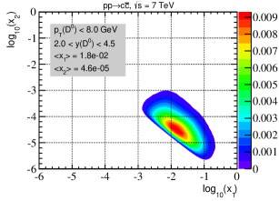
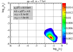
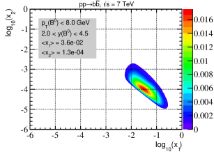
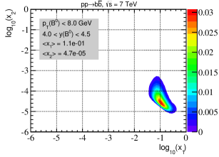
In order to better understand the relation between heavy quark production kinematics and the gluon PDF, it is useful to determine the coverage in the $(x_{1},x_{2})$ plane of the LHCb charm and bottom measurements, where $x_{1}$ and $x_{2}$ are the values of Bjorken-$x$ corresponding to the PDFs in each of the two incoming protons. This coverage is illustrated by the various contour plots shown in Fig. 1. These plots contain the values of $(x_{1},x_{2})$ sampled by the LO calculation of charm (upper) and bottom (lower) production at 7 TeV, within the LHCb acceptance. In the left plots, $D^{0}$ and $B^{0}$ hadrons are required to be within the LHCb rapidity acceptance ($2.0\leq y\leq 4.5$) and have been restricted to a low $p_{T}$ region ($p_{T}<8$ GeV). In the right plots, the hadrons are further restricted in rapidity to the most forward region with $4.0\leq y\leq 4.5$. The calculation has been performed with POWHEG using NNPDF3.0 LO. In all plots, the contours have been normalised to the corresponding fiducial region, and therefore the regions in red indicate where the PDFs are sampled more frequently, while those in blue indicate less frequent sampling. Note that due to the asymmetric acceptance of LHCb, events with $x_{1}\geq x_{2}$, where the first parton is a constituent of the proton travelling in the direction of the LHCb detector (positive rapidity), will be typically selected.

As shown in Fig. 1, measurements of charm production probe average values of Bjorken-$x$ as low as $\left\langle x_{2}\right\rangle\simeq 4.6\cdot 10^{-5}$, and even knowledge of the gluon PDF for values below $x\leq 10^{-5}$ is required for particular bins. This is demonstrated by the plot restricted to the forward region, where $\left\langle x_{2}\right\rangle\simeq 1.5\cdot 10^{-5}$. In this region, there is very limited direct experimental information, since HERA inclusive structure function data [26] is only available down to $x_{\rm min}\sim 6\cdot 10^{-5}$. For this reason, it is of paramount importance to validate our pQCD calculation with the LHCb data itself, since we are using as input PDFs in a region where uncertainties are extremely large. In contrast, the situation for bottom production is under better control since $\left\langle x_{2}\right\rangle\simeq 1.3\cdot 10^{-4}$, a region well covered by the HERA data. This said, for bottom production in the most forward bin, $4.0\leq y\leq 4.5$, we find that $\left\langle x_{2}\right\rangle\simeq 4.7\cdot 10^{-5}$, just below the limit of HERA data, demonstrating that PDF uncertainties also have a sizable impact in this region.

To better illustrate this point, and bearing in mind that heavy quark production at the LHC is driven by the $gg$ luminosity, it is useful to quantify the PDF uncertainties of the NNPDF3.0 gluon, and compare this to other NLO PDF sets. To ease these comparisons, we use the APFEL Web on-line PDF plotter [73, 74]. In Fig. 2 we show a comparison of the gluon PDFs evolved to the scale $Q=1.4$ GeV (corresponding to a typical value of the charm mass) between the NNPDF3.0 and (from top to bottom) the CT10 [20] and MMHT14 [22] NLO PDF sets. In each case, the bands correspond to the 68% confidence level for the PDF uncertainties. The right plots of Fig. 2 show the same comparisons now performed at the scale $Q=4.5$ GeV, a value typical of the bottom quark mass, shown as ratios with respect to the central NNPDF3.0 prediction.

Figure 2: Left plots: comparison of the small-$x$ gluon PDFs at $Q=1.4$ GeV between NNPDF3.0 and (from top to bottom) CT10 and MMHT14. PDFs are compared in an absolute scale, and the bands indicate the PDF uncertainties. Right plots: the same comparisons performed at $Q=4.5$ GeV, now shown as ratios with respect to the central NNPDF3.0 prediction.

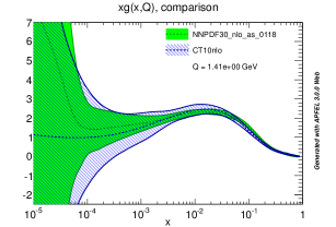
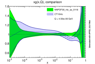
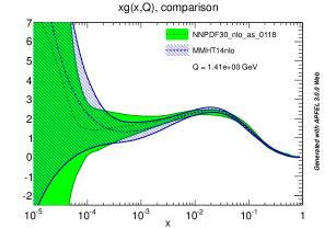
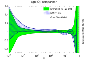
As can be seen, in the region relevant for charm production at LHCb, with $x_{2}\mathrel{\hbox to0.0pt{\lower 4.0pt\hbox{\hskip 1.0pt$\sim$}\hss}\raise 1.0pt\hbox{$<$}}\left\langle x_{2}\right\rangle\simeq 4.6\cdot 10^{-5}$, the gluon PDF uncertainties are extremely large. On the other hand, for the region relevant for bottom production, with $x_{2}\mathrel{\hbox to0.0pt{\lower 4.0pt\hbox{\hskip 1.0pt$\sim$}\hss}\raise 1.0pt\hbox{$<$}}\left\langle x_{2}\right\rangle\simeq 1.3\cdot 10^{-4}$, PDF uncertainties are moderate, thanks to the constraints from HERA data. Importantly, as shown in Fig. 2, the description of the gluon PDF at small-$x$ is quite similar, both in terms of the central value and associated uncertainty — particularly for the comparison between NNPDF3.0 and MMHT sets. As will be shown explicitly, this agreement implies that predictions for charm and bottom production at LHCb obtained with NNPDF3.0 will be similar to those obtained with CT10 or MMHT14 as input PDF sets.

Figure 3: Comparison between the $n_{f}=4$ and $n_{f}=5$ PDFs from the NNPDF3.0 NLO set, as a function of $Q$ for $x=5\cdot 10^{-5}$, in the region relevant for forward charm production at LHCb. We show the gluon (left plot) and the up quark (right plot), normalized to the central value of the $n_{f}=5$ set.

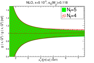
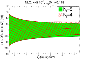
In Fig. 3 we show the comparison between the $n_{f}=4$ and $n_{f}=5$ gluon and up quark NNPDF3.0 NLO PDFs as a function of $Q$, for a reference value $x=2\cdot 10^{-5}$, in the kinematical region relevant for charm production at LHCb. We see that the differences between the $n_{f}=4$ and $n_{f}=5$ schemes are much smaller than the associated PDF uncertainties. We have also explicitly verified that either using $n_{f}=4$ PDFs in the FONLL calculations or including the $n_{f}\to n_{f}+2$ scheme transformation terms in POWHEG leads to negligible modifications of our results. These considerations justify our choice of the NNPDF3.0 NLO $n_{f}=5$ set as baseline in our calculations.

The fact that gluon PDF uncertainties in the region relevant for charm production at LHCb are large indicates that these measurements can be used to provide information on the poorly known small-$x$ gluon. This constraining potential has been recently verified by the PROSA analysis [37] based on the HERAfitter framework [75]. In Sect. 3 we will study the impact of the LHCb charm data in the NNPDF3.0 NLO global analysis using the Bayesian reweighting method.

2.3 Comparison with the LHCb data

We now perform a detailed comparison of the pQCD calculations of charm and bottom production in the forward region with the most recent LHCb data [35, 36]. The comparisons will be performed at the level of double differential distributions,

$${{d^{2}\sigma(D)(y,p_{T})}\over{dy^{D}dp^{D}_{T}}}\quad{\rm and}\quad{{d^{2}\sigma(B)(y,p_{T})}\over{dy^{B}dp^{B}_{T}}}\,.$$ (3)

For all mesons, we have also checked that good agreement is obtained for the total cross-sections in the fiducial region.

For $D$ mesons, we restrict the comparison to the case of the higher-statistics final states, namely $D^{0}$ and $D^{\pm}$, while for the beauty mesons we will show results only for $B^{0}$ production. For each calculation, we provide the central prediction as well as the contribution arising from the various sources of theoretical uncertainty as outlined in Sect. 2.1.

Figure 4: Comparison between the LHCb data on $D$ meson production and the FONLL calculation using NNPDF3.0 as input. We show the results for the most central bin, $2.0\leq y\leq 2.5$ (left column) and a forward bin, $3.5\leq y\leq 4.0$ (right column), both for $D^{0}$ data (upper row) and the $D^{\pm}$ data (lower row). The solid error band is obtained from the sum in quadrature of PDF and scale uncertainties, while the hatched band is only the scale variation component.

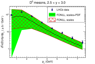
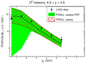
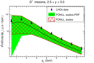
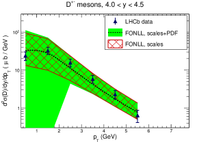
The comparison between the FONLL calculation and the LHCb charm production data is shown in Fig. 4. We show the results for the most central bin, $2.0\leq y\leq 2.5$ and a forward bin, $3.5\leq y\leq 4.0$, both for the $D^{0}$ and the $D^{\pm}$ measurements. In Fig. 4, statistical and systematic uncertainties have been added in quadrature for the experimental data, while for the theory uncertainties we show both the scale uncertainty alone and also the sum in quadrature of scale and PDF uncertainties.

The agreement, within uncertainties, between the LHCb data and the NLO pQCD prediction across the entire kinematic range demonstrates the applicability of this approach to forward charm production. The total theoretical uncertainty is dominated by scale variation, except in the low $p_{T}$ where the large gluon PDF uncertainty at small-$x$ becomes comparable to the scale variation or even dominant. Similar satisfactory agreement is found for the other data bins not shown in Fig. 4.

Figure 5: Comparison between the FONLL and aMC@NLO (upper plots) and between the POWHEG and aMC@NLO (lower plots) calculations for $D^{0}$ production in the same kinematics as the LHCb data of Fig. 4, using NNPDF3.0 NLO. The total theory uncertainly band is obtained by the addition in quadrature of scale and PDF uncertainties.

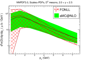
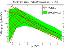
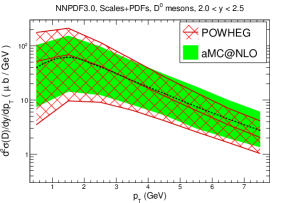
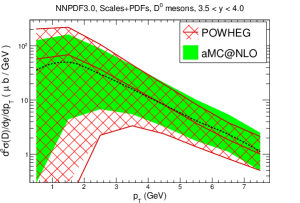
Given the compatibility of the charm production data and theory prediction provided by FONLL, we now compare these predictions to those obtained with the NLO Monte Carlo approaches, aMC@NLO and POWHEG. First of all we compare the FONLL results with the aMC@NLO calculation. For simplicity, we only provide results for $D^{0}$ mesons. The comparison is shown in Fig. 5: clearly, there is good agreement between the central values of the two calculations. For the total theory uncertainty band there is also reasonable agreement, with the aMC@NLO band being typically larger than, but still consistent, with the FONLL result. In this comparison the theory uncertainty band is obtained from adding scale and PDF uncertainties in quadrature. The corresponding comparison between the two MC generators, aMC@NLO and POWHEG, is shown in the lower plots of Fig. 5. Reasonable agreement is also found between the central predictions, well within the uncertainty bands. We note that scale uncertainties tend to be slightly larger in the POWHEG calculation.

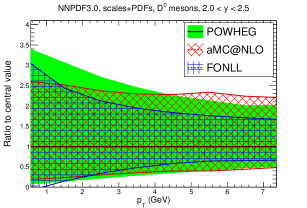
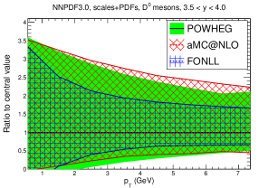
In Fig. 6 we perform the same comparison between the three calculations as shown in Fig. 5, but now normalising each prediction to the corresponding central value. This way we can gauge how the total theory uncertainty band compares among the three calculations. The total uncertainty is similar for POWHEG and aMC@NLO calculations. Notably, the scale uncertainties of the POWHEG and aMC@NLO calculations tend to be larger than those of FONLL, especially in the upper variations in the moderate and high $p_{T}$ region. While the origin of these differences remains to be understood, it might be related to the fact that FONLL is a fixed-order calculation while POWHEG and aMC@NLO are matched to parton showers, and this matching may induce additional theoretical uncertainties. Indeed, we have verified that the scale uncertainties of the fixed-order NLO computation of differential $c\bar{c}$ production (without fragmentation) in aMC@NLO reproduces those of FONLL to a few percent.

From Fig. 6 we see that the FONLL semi-analytical calculation exhibits smaller theoretical uncertainty, and for this reason, in the following Section we will use the FONLL predictions to quantify the constraints of the LHCb charm production data on the NNPDF3.0 small-$x$ gluon PDF.

Figure 6: Comparison between the total theoretical uncertainty (sum in quadrature of scale and PDF uncertainties) for the kinematics of $D^{0}$ production at LHCb. The results for the three calculations, aMC@NLO, POWHEG, and FONLL calculations, are normalised to the respective central values.

We now begin the comparison between the LHCb data and the various theoretical calculations for the case of $B$ meson production. For simplicity, we show results only for $B^{0}$ mesons, though similar agreement has been found for the other $B$ mesons. As compared to the case of the $D$ mesons, we expect a reduction of the theory uncertainties for several reasons: the calculation is performed at a higher scale $\sqrt{m_{b}^{2}+p_{T,b}^{2}}$, as compared to the charm production case, $\sqrt{m_{c}^{2}+p_{T,c}^{2}}$, leading to an improved convergence of the perturbative expansion; the relative uncertainty of the value of $m_{b}$ is smaller; and larger values of $x_{1,2}$ are probed within the proton, a region well covered by HERA data as illustrated in Fig. 1 and Fig. 2.

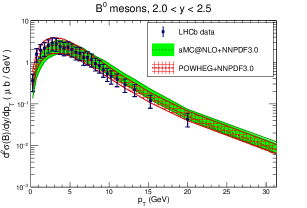
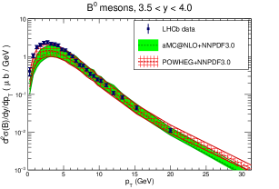
In Fig. 7 we show the comparison of the LHCb data for $B^{0}$ meson production, both for central and for forward rapidities, with the corresponding POWHEG and aMC@NLO calculations. The indicated theory uncertainty band includes only the scale uncertainties, and we have verified that PDF uncertainties are not so relevant in this case. As in the case of charm, satisfactory agreement between theory and data for $B$ meson production in the forward region is found. There is also a substantial reduction of the theory uncertainty as compared to the $D$ meson case. The POWHEG and aMC@NLO predictions are in reasonable agreement within the theory uncertainty band.

Figure 7: Comparison of the LHCb data on $B^{0}$ meson production, both for central and for forward rapidities, with the theoretical predictions from POWHEG and aMC@NLO. The theory uncertainty includes only scale uncertainties.

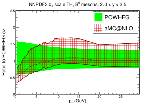
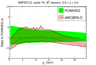
To better assess the differences between the two NLO matched calculations, we compare them again in Fig. 8, this time with the distributions normalised to the central POWHEG prediction. The aMC@NLO and POWHEG predictions agree across the considered kinematic range, with the POWHEG prediction favouring a slightly larger cross section in the low $p_{T}$ range. In comparison to the charm results, Fig. 6, the reduction of scale uncertainties is evident, since now the scale variation amounts to an uncertainty of $\simeq 40\%$. We can conclude that the pQCD description of $B$ meson production in the forward region is completely satisfactory, and that theory uncertainties are substantially reduced as compared to charm production.

Figure 8: Comparison of the theoretical predictions for $B^{0}$ meson production at the LHCb kinematics between POWHEG and aMC@NLO, shown in Fig. 7, but now where calculations are normalised to the central value of the POWHEG prediction.

In this section we have restricted our study to 7 TeV, the only centre-of-mass energy for which LHCb measurements are currently available. Predictions for double differential distributions at 13 TeV, as well as for the ratio of cross-sections at computed at 13 over 7 TeV, will be provided in Sect. 4.1 and 4.2.

2.4 PDF dependence of heavy quark production at LHCb

The results shown so far in this Section have been computed using the NNPDF3.0 NLO set. We have verified that the pQCD predictions for heavy quark production are affected by a sizeable PDF uncertainty, which arises in turn from poor knowledge of the small-$x$ gluon PDF due to a lack of direct experimental constraints. In this section we study the dependence of our predictions on the choice of input PDF set, in particular we compare those of the baseline NNPDF3.0 to CT10 and MMHT14 NLO sets. The comparison of the small-$x$ gluon PDF between these three sets shown in Fig. 2 indicates that predictions for charm production cross-sections are expected to be reasonably similar.

In Fig. 9 we show the comparison of the theoretical predictions for charm production at 7 TeV within the LHCb acceptance found using the POWHEG calculation with NNPDF3.0, CT10 and MMHT14 PDFs. The uncertainty band corresponds to the 68% confidence level for each PDF set, and the shown results have been normalised to the central value of the NNPDF3.0 prediction. From this comparison, we see that the dependence of the charm cross-section on the choice of input PDF set is moderate, with the three central values consistent within large PDF uncertainties. Recall that at fixed rapidity, smaller values of the $D$ meson $p_{T}$ correspond to probing smaller $x$ values for the gluon PDF, and that, likewise, for a fixed value of $p_{T}$, forward rapidities corresponds to smaller $x$ values. It is therefore reasonable that PDF uncertainties are largest at small $p_{T}$ and forward rapidities, as shown in Fig. 9.

Figure 9: Comparison of the theoretical predictions for $D^{0}$ meson production at $\sqrt{s}$=7 TeV in the LHCb kinematics with POWHEG, for three different NLO sets of PDFs, NNPDF3.0, CT10 and MMHT14. The band corresponds to the respective one-sigma PDF uncertainty for each set. Results are shown normalised to the central value of the NNPDF3.0 prediction.

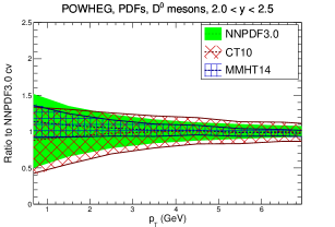
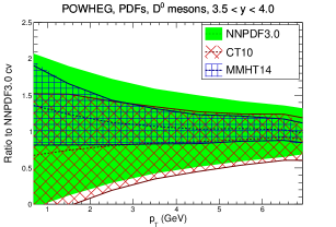
Even though predictions suffer from large PDF uncertainties, the central value of these three PDF sets are reasonably consistent. This agreement can in part be explained by the fact that at small-$x$ PDF constraints in the three sets come from the same dataset, the combined HERA-I measurements [26]. We note that the relative size of the PDF uncertainties is similar for NNPDF3.0 and CT10, while the MMHT14 uncertainty is about a factor of two smaller. Another feature of these predictions is the preference for the CT10 and MMHT14 central values towards relatively smaller and larger differential cross sections for small $p_{T}$ values, respectively. This can be traced to the relatively softer and harder gluon PDF at small-$x$ preferred by the CT10 and MMHT14 respectively as compared to NNPDF3.0 — see Fig. 2.

We conclude from Fig. 9 that although there is some dependence on the choice of input PDF set, these differences are small within the large intrinsic PDF uncertainties, and therefore it is sufficient to use a single PDF set, NNPDF3.0, as baseline in our calculations.

3 Constraints on the small-$x$ gluon PDF from forward charm production data

As demonstrated in the previous section, the production of charmed hadrons in the forward region and the associated theoretical uncertainty depends on the description of the gluon PDF at small-$x$. We now use the charm production data from LHCb to substantially reduce the small-$x$ gluon PDF uncertainties. This will allow a more reliable prediction for both forward charm production at the LHC Run II and the prompt neutrino cross section arising from high energy cosmic rays — an important input for calculating the background neutrino flux at IceCube.

The basic idea is similar to the study performed by the PROSA Collaboration [37], where the impact of forward $B$ and $D$ LHCb data on the low-$x$ PDFs is studied. The PROSA study is based on the HERAfitter framework [75], and quantifies the error reduction in a HERA-only PDF fit when the LHCb $B$ and $D$ meson production data is included using the MNR code [46] in a FFN $N_{f}=3$ scheme. Similarly as will be done here, theoretical uncertainties can be reduced by suitable normalisations. This said, there are important methodological differences in the two analysis (global fit versus HERA-only fit, theory calculations, data normalisation strategies), and so the two approaches complement one another.

The starting point is the NNPDF3.0 NLO set, with $\alpha_{s}(m_{Z})=0.118$, supplemented by the LHCb measurements of the 7 TeV differential distributions for $D^{0}$ and $D^{\pm}$ production [36]. The LHCb data will be added to the NNPDF3.0 global dataset by means of the Bayesian reweighting technique [39, 40]. This method allows to quantify the impact of new data in a set of Monte Carlo PDFs without the need of redoing the full global QCD analysis, and has been used before in a number of related applications in order to quantify the impact on PDF fits from data for isolated photon production [77, 78], top quark pair production [79], and polarised $W^{\pm}$ and jet production [80]. As an alternative to the reweighting, it should also have been possible to use the aMCfast [81] interface to construct an APPLgrid [82] fast implementation of the aMC@NLO calculations presented in the previous section.

As input to the reweighting, we consider the $\left(y,p_{T}\right)$ double differential distributions for $D^{0}$ and $D^{\pm}$ production at LHCb, but exclude the data from other final states such as $D^{*\pm}$ and $D^{\pm_{s}}$ which are affected by larger experimental uncertainties, and therefore have reduced impact on the fit. These data cover a range in rapidity of $[2.0,4.5]$ and in $p_{T}$ of $[0,8]$ GeV. In total, we are adding $N_{\rm dat}=75$ new data points into the NNPDF3.0 analysis.

For the theoretical calculations, we use the FONLL predictions, with the settings discussed in the previous Section. In Fig. 10 we compare the LHCb charm production data and the FONLL prediction for the $D^{0}$ and $D^{\pm}$ data. Results are shown normalised to the central value of the respective experimental data point. The experimental statistical and systematic uncertainties have been added in quadrature, and both scale and PDF uncertainties are independently shown for the FONLL theoretical prediction.

Figure 10: Comparison between the LHCb charm production data and the FONLL calculation with NNPDF3.0 NLO at the level of unnormalized (absolute) cross-sections. The left plot shows the $D^{0}$ data while the right plot corresponds to the $D^{\pm}$ data. Results are shown normalised to the central value of the LHCb data. For the FONLL calculation we show separately the scale and the PDF uncertainties. The data is ordered in increasing rapidity bins, an within each of these, in increasing $p_{T}$ bins.

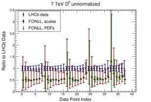
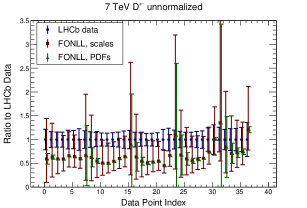
It is clear by inspection of Fig. 10 that the scale uncertainties in the NLO calculation are large, by as much as a factor of two for some bins. In general, they are reduced when going towards higher $p_{T}$ bins, thanks to the improved convergence of the perturbative expansion in this region. Although PDF uncertainties are also large, especially at low $p_{T}$ and forward rapidities where the small-$x$ gluon is being probed, they are sub-dominant as compared to the scale uncertainties. This is concerning from the point of view of a PDF analysis, in which a scale choice for the central value of the theory prediction must be made.

To bypass this problem, the strategy that will be adopted in this work is to normalise all the data bins to that with highest $p_{T}^{D}$, $\left[7,8\right]$ GeV, and central rapidity $y^{D}$, $\left[2.0,2.5\right]$. The rationale for this choice is that scale uncertainties will partially cancel in the ratio, while the cancellation of PDF uncertainties will not be as severe, given that different bins in $\left(y^{D},p_{T}^{D}\right)$ probe different values of $(x,Q^{2})$ of the gluon PDF. The reference bin has been chosen precisely for this reason, as PDF uncertainties for this particular bin are the smallest. Note that this is strategy is different as compared to the PROSA analysis [37], where, separately for each bin in $p_{T}^{D}$, the rapidity bin $3.0\leq y^{D}\leq 3.5$ was used to normalize the data and the theory calculations.

In Fig. 11 we provide the same comparison of Fig. 10, but this time at the level of normalised distributions. In Fig. 11 we have added in quadrature the experimental uncertainties in the numerator and the denominator, this being the only option since the full experimental covariance matrix with the information of correlations between bins is not available. Theoretical uncertainties are taken to be fully correlated among all the data bins.

Figure 11: Same as Fig. 10, where now both data and theory have been respectively normalised with respect to the bin with $7~{}{\rm GeV}\leq p_{T}\leq 8$ GeV and $2.0\leq y\leq 2.5$ (the bin with data point index 8).

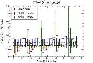
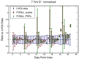
The comparison between Fig. 10 and Fig. 11 illustrates how after the normalisation procedure has been applied, scale uncertainties are substantially reduced in the low-$p_{T}$ and large-$y$ bins. Importantly, the PDF uncertainties are now larger than the corresponding scale and experimental uncertainties in these bins, which justifies the inclusion of the normalised charm production cross-sections into NNPDF3.0 using Bayesian reweighting. In this respect, after the normalisation, the theoretical status of forward charm production becomes similar to that of other hadronic processes routinely included in global NLO fits, such as jet production.

The results of the reweighting are summarised in Table 1. The breakdown of the $\chi^{2}$ per data point of the $D^{0}$ and $D^{\pm}$ data before and after reweighting, as well as the number of effective replicas left out of the original $N_{\rm rep}=100$ replicas, is provided. The description of the normalised LHCb charm data turns out to be excellent even using the original NNPDF3.0 set, with a value of $\chi^{2}/N_{\rm dat}=1.10$. This is certainly reassuring, since it shows that both NNPDF3.0 and the FONLL calculation provide a good description of charm production in the LHCb acceptance. Once the data is included by the reweighting, the $\chi^{2}_{\rm rw}/N_{\rm dat}=0.74$ is even better, and the effective number of replicas is $N_{\rm eff}=50$, confirming that this data is indeed very constraining on the small-$x$ gluon PDF. Note that since we are neglecting the correlations between systematics, we are underestimating the impact of these data. Future measurements with the full systematic breakdown should be even more powerful.

	NNPDF3.0	NNPDF3.0+LHCb data
$\chi^{2}/N_{\rm dat}$ for $D^{0}$ + c.c.	1.13	1.05
$\chi^{2}/N_{\rm dat}$ for $D^{+}$ + c.c.	1.06	0.40
$\chi^{2}/N_{\rm dat}$ for $D^{0}$ + $D^{\pm}$	1.10	0.74
$N_{\rm eff}$ for $D^{0}$ + $D^{\pm}$	-	50

Table 1: Results of the reweighting of NNPDF3.0 with the LHCb charm production data. We give the value of the $\chi^{2}/N_{\rm dat}$, both for the original NNPDF3.0 set, and for the reweighted NNPDF3.0+LHCb set, as well as the effective number of replicas left, $N_{\rm eff}$.

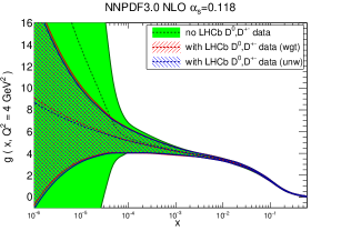
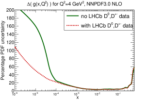
The impact of the LHCb charm production data into the small-$x$ gluon PDF can be seen in Fig. 12. We show the NNPDF3.0 small-$x$ gluon, evaluated at $Q=2$ GeV, compared with the new gluon obtained after the inclusion in the fit of the normalised LHCb charm data. As a cross-check, we have also verified that it is possible to unweight the results to produce a stand-alone LHAPDF6 grid for the combined NNPDF3.0+LHCb fit (indicated as “(unw)” in the plot legend). In Fig. 12 we also compare the percentage PDF uncertainties for the NNPDF3.0 gluon with and without the inclusion of the LHCb data, which quantify the reduction of PDF uncertainties at small-$x$.

We see that the impact of LHCb data is negligible for $x\mathrel{\hbox to0.0pt{\lower 4.0pt\hbox{\hskip 1.0pt$\sim$}\hss}\raise 1.0pt\hbox{$>$}}10^{-4}$, where most of the HERA data is available, but becomes substantial for $x\mathrel{\hbox to0.0pt{\lower 4.0pt\hbox{\hskip 1.0pt$\sim$}\hss}\raise 1.0pt\hbox{$<$}}10^{-4}$, where the previously large PDF uncertainties are dramatically reduced. For instance, for $x\sim 10^{-5}$, the PDF uncertainties in the gluon PDF are reduced by more than a factor three. We also note that the central value at small-$x$ of the gluon PDF preferred by the LHCb charm data is less steep than that of the global fit, although fully consistent within uncertainties. The quark PDFs are essentially unaffected by the inclusion of the LHCb charm data and are thus not shown here.

Figure 12: Left: The NNPDF3.0 NLO small-$x$ gluon, evaluated at $Q=2$ GeV, comparing the global fit result with with the new gluon obtained from the inclusion of the LHCb charm production data. In the latter case, we show both the reweighted (rwg) and the unweighted (unw) results. Right: comparison of percentage PDF uncertainties for the NNPDF3.0 gluon with and without the inclusion of the LHCb data, computed also at $Q=2$ GeV, that illustrate the reduction of PDF uncertainties for $x\mathrel{\hbox to0.0pt{\lower 4.0pt\hbox{\hskip 1.0pt$\sim$}\hss}\raise 1.0pt\hbox{$<$}}10^{-4}$.

Since the resulting PDF set from the inclusion of the LHCb data into NNPDF3.0 has been unweighted to a a LHAPDF6 grid, it can be easily used both for the predictions of heavy quark production at 13 TeV at LHCb, presented in Sect. 4, and for the prompt neutrino cross-sections relevant for IceCube in Sect 5.

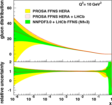
It is interesting to assess how the results of this analysis compare to those of the PROSA study [37]. Note that the two analysis use rather different methodologies (HERA-only fit versus global fit, HERAfitter versus NNPDF reweighting), and given that this is the first time that forward charm data is used in a PDF fit, it is important assess the robustness of the results by performing a cross-check. Since the PROSA analysis is performed in the FFN $n_{f}=3$ scheme, we have constructed a FFN $n_{f}=3$ version of the NNPDF3.0+LHCb NLO set using APFEL [73]. The results of this comparison are shown in Fig. 13, where we show the gluon PDF at $Q^{2}=10$ GeV² in the FFN scheme with $N_{f}=3$, In the PROSA case, we show the results both in the HERA-only fit and in the HERA+LHCb fit. The lower panel compares the relative PDF uncertainties in each case. As can be seen, there is good agreement both between central values (the two gluons agree within their one-sigma band) and especially between PDF uncertainties, which is a non-trivial verification of the two analyses.

Figure 13: The gluon PDF at $Q^{2}=10$ GeV² in the FFN scheme with $N_{f}=3$, comparing the results of this work with those of the PROSA analysis. In the latter case, we show the results both in the HERA-only fit and in the HERA+LHCb fit. The lower panel compares the relative PDF uncertainties in each case.

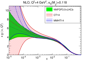
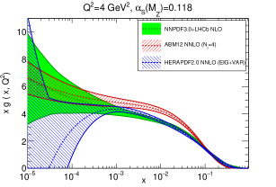
Finally, let us compare the resulting gluon PDF in this analysis with those of other recent PDF fits. In Fig. 14 we compare the NNPDF3.0+LHCb gluon PDF at $Q^{2}=4$ GeV² with the CT14 [85] and MMHT14 results (left plot), and to the ABM12 [84] and HERAPDF2.0 [86] results (right plot). In the case of HERAPDF2.0, both the experimental, model and parametrization uncertainties are included. In the case of ABM12, the $n_{f}=4$ set has been adopted. From Fig. 14 we note that the NNPDF3.0+LHCb central value is close to the CT14 result, but with much smaller uncertainties, while the MMHT14 gluon is substantially larger at small-$x$. From the comparison with ABM12 we find reasonable agreement for $x\leq 10^{-4}$, while HERAPDF2.0 predicts a much smaller (negative gluon), though consistent with the NNPDF3.0+LHCb result within the PDF large uncertainties.

Figure 14: The NNPDF3.0+LHCb gluon PDF at $Q^{2}=4$ GeV² compared with CT14 and MMHT14 (left plot), and to ABM12 and HERAPDF2.0 (right plot). In the case of HERAPDF2.0, both the experimental, model and parametrization uncertainties are included.

4 Predictions for 13 TeV and for the 13/7 TeV ratio

In this section we provide predictions for $D$ and $B$ production within the LHCb acceptance at 13 TeV. We also provide predictions for the ratio of differential cross-sections between 13 and 7 TeV. Our predictions are have been computed using the POWHEG and aMC@NLO calculations with the improved NNPDF3.0+LHCb PDF set constructed in Sect. 3, and can be used to compare with the upcoming Run II measurements at LHCb. Using the theoretical value of the ratio between inclusive fiducial cross-sections at 13 and 7 TeV, and the LHCb 7 TeV data ($R_{13/7}$), we also provide predictions for $B$ and $D$ mesons in fiducial cross-sections at 13 TeV. A tabulation of our results is provided in Appendix A, and predictions for different binning choices and other meson species are available from the authors on request.

4.1 Forward heavy quark production at 13 TeV

First of all, we provide theory predictions required to compare with the upcoming LHCb data on charm and bottom production which will be collected at 13 TeV. Our results are presented according to the binning scheme adopted in the 7 TeV measurements [36, 35], with the exception that a slightly finer binning for the charm predictions is chosen at low $p_{T}$ and the high $p_{T}$ range is slightly extended. For all predictions, the uncertainty due to scales, PDFs, and the heavy quark mass is provided as a sum in quadrature.

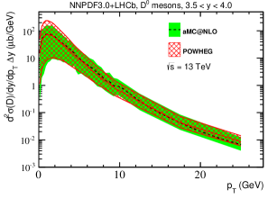
In Fig. 15, the double differential distributions for $D^{0}$ mesons at 13 TeV are shown for both a central and a forward rapidity bin within the LHCb acceptance. The central value and total uncertainty of both POWHEG and aMC@NLO calculations are provided. This comparison demonstrates that there is good agreement between the two calculations, both in terms of central values and in terms of the total uncertainty band — agreement also holds for other $D$ mesons and rapidity regions, which are not shown here. Thanks to using the improved NNPDF3.0 PDFs with 7 TeV LHCb data, PDF uncertainties turn out to be moderate even at 13 TeV, with scale variations being the dominant source of theoretical uncertainty.

Figure 15: The double-differential distribution, $d^{2}\sigma(D)/dydp_{T}$, for the production of $D^{0}$ mesons at LHCb for a centre-of-mass energy of 13 TeV. We show representative results for the central ($2.0\leq y\leq 2.5$) and forward ($3.5\leq y\leq 4.0$) regions. We compare the POWHEG and aMC@NLO calculations, using the NNPDF3.0+LHCb PDF set. For both calculations, the theory uncertainty band is computed adding in quadrature scales, PDF and charm mass uncertainties.

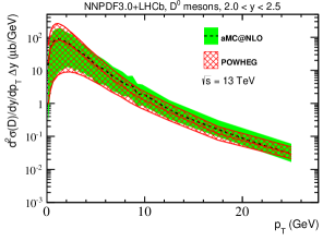
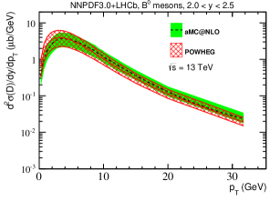
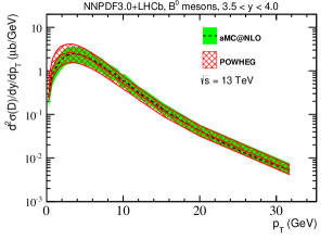
The corresponding comparison for $B^{0}$ mesons is shown in Fig. 16. As in the case of the charm, there is excellent agreement between the POWHEG and aMC@NLO calculations within the LHCb acceptance.

Figure 16: Same as Fig. 15 for $B^{0}$ mesons.

The tabulation of the results shown in Figs. 15 and 16 are provided in Appendix A, in particular in Tables 3 (for $D^{0}$ mesons) and 4 (for $B^{0}$ mesons).

4.2 Predictions for the ratio between the 13 and 7 TeV cross-sections

In addition to differential cross section measurements, it will also become possible to measure the ratio of differential cross sections performed at 13 and 7 TeV when the 13 TeV data is available. As discussed in Ref. [41], measurements of the ratio of cross-sections at different centre-of-mass energies are well motivated as many theoretical uncertainties, such as scale uncertainties, mass dependence, and fragmentation/branching fractions cancel in the ratio to a good approximation. In addition, many experimental uncertainties also cancel in such ratios which allows stringent tests of the Standard Model to be performed. The relevance of the ratio of 13 over 7 TeV heavy quark production cross-sections at LHCb for PDF studies has also been recently emphasised in Ref. [89], in a study of the various theoretical uncertainties associated to charm and bottom production in the forward region.

On the other hand, PDF uncertainties do not cancel completely, because of the different kinematical range covered by the measurements at the two centre-of-mass energies, and thus these ratio measurements provide in principle useful PDF discrimination power. This idea has been implemented already by a number of LHC analyses, like the ATLAS measurement of the ratio of 7 TeV over 2.76 TeV jet cross-sections [83] and the CMS measurement of the ratio of 8 TeV over 7 TeV Drell-Yan distributions [88].

In Fig. 17 we show the predictions for the ratio of differential cross-sections for $D^{0}$ production between 13 TeV and 7 TeV, defined as

$$R_{13/7}^{D^{0}}(y^{D},p_{T}^{D})\equiv{{d^{2}\sigma(D^{0})(y^{D},p_{T}^{D},13~{}{\rm TeV})}\over{dy^{D}dp_{T}^{D}}}\Bigg{/}{{d^{2}\sigma(D^{0})(y^{D},p_{T}^{D},7~{}{\rm TeV})}\over{dy^{D}dp_{T}^{D}}}\,,$$ (4)

where the same binning as in the 7 TeV LHCb measurement has been assumed. In the left plot we show the results computed with POWHEG and the NNPDF3.0+LHCb PDF set, for each of the bins of the 7 TeV measurement (data points are ordered in increasing bins of rapidity, and within each of these five rapidity bins, in increasing bins of $p_{T}$). The central value of the ratio $R_{13/7}^{D^{0}}$ varies between 1.20 and 2.2 for increasing values of $p_{T}$ and more forward rapidity bins, where the opening of phase space between 13 TeV with respect to 7 TeV is more important.

Figure 17: Left plot: predictions for the ratio of differential cross-sections $R_{13/7}^{D^{0}}$, Eq. (4), for the production of $D^{0}$ mesons between 13 TeV and 7 TeV, computed using POWHEG and NNPDF3.0+LHCb. Results are ordered in increasing bins in rapidity, in within each, in increasing bins of $p_{T}$. The total theoretical uncertainty in the ratio is decomposed into its various sources: scale, PDF and charm quark mass variations. Right plot: comparison of the predictions for $R_{13/7}^{D^{0}}$ between POWHEG and aMC@NLO, for central values and for the total theory uncertainties.

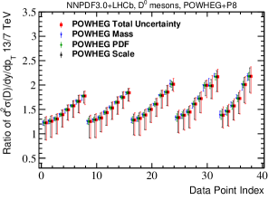
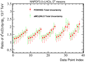
In the left plot of Fig. 17 we have separated the total theory uncertainty into the individual contributions from scales, PDFs and charm mass to highlight their importance. We see that the total uncertainty in $R_{13/7}^{D^{0}}$ varies between 10% and 30%, depending on the specific bin, and that scale variation is found to dominate the total uncertainty in $R_{13/7}^{D^{0}}$. Note however the substantial cancellation of scale uncertainties as compared to the absolute differential cross-sections shown in Fig. 15. In Appendix A we provide a tabulation of the results of Fig. 17, which will be useful for comparison if the ratio $R_{13/7}^{D^{0}}$ is measured in the upcoming LHCb 13 TeV analysis. In the same appendix we also quantify the reduction of PDF uncertainties in $R_{13/7}^{D^{0}}$ by comparing the predictions using the original NNPDF3.0 set with our baseline predictions obtained with NNPDF3.0+LHCb. The substantial reduction of PDF uncertainties in $R_{13/7}^{D^{0}}$, thanks to the constraints from the 7 TeV normalised charm cross-sections derived in Sect. 3, improve the robustness of our theory prediction for $R_{13/7}^{D^{0}}$. Conversely, the measurement of $R_{13/7}^{D^{0}}$ should provide important PDF discrimination power, and it would be interesting to verify the consistency of the constraints on the small-$x$ gluon from $R_{13/7}^{D^{0}}$ from those that we have derived from the normalised 7 TeV data.

To validate the cancellation of the theoretical systematics in the POWHEG calculation, we have also computed the ratio with the aMC@NLO calculation. The comparison of these two calculations, including their total uncertainties, is shown in the right plot of Fig. 17. Reasonable agreement is found, both for the central values and for the uncertainties. In particular, for most of the bins, the central predictions for $R_{13/7}^{D^{0}}$ agree within 10% at most. This agreement should be considered satisfactory especially taking into account the very large theory uncertainties in the absolute distributions.

Next we provide the corresponding predictions for the ratio of $B$ meson differential distributions between 13 TeV and 7 TeV, defined as

$$R_{13/7}^{B^{0}}(y^{B},p_{T}^{B})\equiv{{d^{2}\sigma(B^{0})(y^{B},p_{T}^{B},13~{}{\rm TeV})}\over{dy^{B}dp_{T}^{B}}}\Bigg{/}{{d^{2}\sigma(B^{0})(y^{B},p_{T}^{B},7~{}{\rm TeV})}\over{dy^{B}dp_{T}^{B}}}\,,$$ (5)

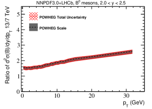
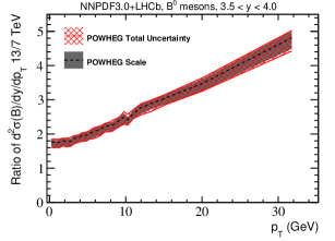
for the case of $B^{0}$ mesons, which we choose for illustrative purposes. In Fig. 18 we show the theoretical predictions for the ratio $R_{13/7}^{B^{0}}$ computed with POWHEG using NNPDF3.0+LHCb for two representative bins in rapidity, one central (left plot) and one forward (right plot), as a function of $p_{T}^{B}$. The total theory uncertainty (hatched band) is compared with the scale uncertainty (solid band). We have verified that the results for $R_{13/7}^{B^{0}}$ obtained with aMC@NLO are fully consistent the POWHEG calculation. In the results of Fig. 18, the same binning as in the 7 TeV measurement has been used [36].

From Fig. 18 we see that $R_{13/7}^{B^{0}}$ varies between 1.3 at central rapidities at low $p_{T}$ to almost 5 at forward rapidities and large $p_{T}$, for the same reasons as $R_{13/7}^{D^{0}}$. The total uncertainty in $R_{13/7}^{B^{0}}$ ranges between 5 and 10%, depending on the specific bin, and is dominated by the scale uncertainty (but only due to using the improved NNPDF3.0+LHCb set). As in the case of charm production, in Appendix A we tabulate our predictions for $R_{13/7}^{B^{0}}$, that can be used to compare the the upcoming LHCb measurement. The corresponding predictions for other $B$ meson species are available upon request.

Figure 18: Theoretical predictions for the ratio $R_{13/7}^{B^{0}}$ Eq. (5) between $B^{0}$ meson distributions between 13 and 7 TeV. Results have been computed with POWHEG using NNPDF3.0+LHCb. We show the predictions for two representative bins in rapidity, one central (left plot) and the other forward (right plot), as a function of $p_{T}^{B}$. The total theory uncertainty (hatched band) is compared with the scale uncertainty (solid band).

4.3 Predictions for inclusive fiducial cross-sections at 13 TeV

In addition to the double differential distributions, it is also useful to provide predictions for the charm and bottom inclusive cross-section, that is, the cross-sections measured within the full LHCb fiducial region. In the case of $D$ mesons, the fiducial region is defined as

$$0\leq p_{T}^{D}\leq 8~{}{\rm GeV}\,,\qquad 2.0\leq y^{D}\leq 4.5\,,$$ (6)

while the corresponding fiducial region for the production of $B$ mesons is defined by

$$0\leq p_{T}^{B}\leq 40~{}{\rm GeV}\,,\qquad 2.0\leq y^{B}\leq 4.5\,.$$ (7)

In order to compute the 13 TeV predictions for the charm and bottom inclusive cross-sections in the fiducial region, there are two possible strategies that can be adopted, namely

• integrating the POWHEG calculation for the absolute double differential cross-sections, shown in Fig. 15, for the acceptance in Eq. (6), or instead

• using the theoretical predictions for the ratios $R_{13/7}^{D}$ and $R_{13/7}^{B}$ to rescale the corresponding 7 TeV LHCb inclusive measurements reported in [36, 35].

The main advantage of the second option is that theoretical uncertainties are substantially reduced in the ratios $R_{13/7}^{D}$ and $R_{13/7}^{B}$ as compared to the absolute cross-sections, allowing a reasonably accurate extrapolation for the 13 TeV inclusive cross-sections, with precision comparable to that expected for the corresponding experimental measurement.

Let us illustrate how the two strategies compare in the case of $D$ meson production. For simplicity, we will show the results for $D^{0}$ mesons but the same ideas apply to the other $D$ mesons. In this case, the prediction for the inclusive ratio, with the total associated theory uncertainty, is given by

$$R_{13/7}^{D^{0}}({\rm th,incl})=1.39\,~{}^{+0.12\,(8.3\%)}_{-0.29\,(20.5\%)}\,.$$ (8)

This can be combined with the 7 TeV LHCb inclusive measurement [36] in the fiducial region for $D^{0}$ mesons

$$\sigma^{D^{0}}_{\rm 7TeV}({\rm LHCb,incl})=1661\pm 129\,~{}(\pm 7.8\%)\,~{}{\rm\mu b}\ ,$$ (9)

to obtain an accurate prediction for the corresponding 13 TeV inclusive cross-section in the same fiducial region. This leads to

$$\sigma^{D^{0}}_{\rm 13TeV}({\rm th,incl})=\sigma^{D^{0}}_{\rm 7TeV}({\rm LHCb,incl})\cdot R_{13/7}^{D^{0}}({\rm th,incl})=2236^{+308\,(14\%)}_{-521\,(23\%)}\,~{}{\rm\mu b}\ ,$$ (10)

where the theoretical uncertainty from $R_{13/7}^{D^{0}}$ is slightly larger than that of the 7 TeV measurement, and dominates the precision of the prediction for $\sigma^{D^{0}}_{\rm 13TeV}$ performed in this way. In Eq. (10) we have added in quadrature the theory uncertainties from $R_{13/7}^{D^{0}}$ with the experimental uncertainties of the LHCb measurement.

In Table 2 the prediction for the inclusive cross-section $\sigma^{D^{0}}_{\rm 13TeV}$ obtained using the 7 TeV measurement and the calculation of $R_{13/7}^{D}$ is compared to the corresponding result computed from the integral of the absolute differential distributions. The advantage of the ratio strategy is apparent: when integrating the absolute distributions, the prediction is affected by large theory uncertainties up to 200% which render the comparison with the much more accurate experimental measurement not very informative. On the other hand, our prediction obtained using $R_{13/7}^{D}$ has a 10-20% accuracy, comparable to that of the upcoming Run II LHCb measurement, and therefore should provide interesting information for the comparison between data and theory in a hitherto unexplored kinematical region. In Table 2 we also provide the predictions for the inclusive charm pair production cross-section using the two methods, obtained from rescaling the meson-level result by the branching fraction of charm into $D^{0}$ mesons,

$$\sigma^{c\bar{c}}_{\rm 13TeV}({\rm th,incl})=\sigma^{D^{0}}_{\rm 13TeV}({\rm th,incl})/\left(2f\left(c\to D^{0}\right)\right)\,.$$ (11)

This prediction is useful to compare with parton-level predictions of charm production, which do not account for the fragmentation of charm quarks into $D$ mesons.

13 TeV	$D^{0}$			$c\bar{c}$
$\sigma_{\rm 13TeV}({\rm th,incl})(\mu b)$ (from ratio)	2236		${}^{+308\,(14\%)}_{-521\,(23\%)}$	1979		${}^{+249\,(13\%)}_{-447\,(23\%)}$
$\sigma_{\rm 13TeV}({\rm th,incl})(\mu b)$ (from abs)	1097		${}^{+2082\,(190\%)}_{-896\,(82\%)}$	970		${}^{+1843\,(190\%)}_{-793\,(82\%)}$

Table 2: Predictions for the inclusive $D^{0}$ production cross-section in the fiducial region Eq. (6) at 13 TeV using the two methods discussed in the text (integrating the absolute distributions and rescaling the 7 TeV LHCb measurement with the ratio $R^{D}_{13/7}$). Predictions are also provided for the corresponding $c\bar{c}$ cross-sections using Eq. 11.

The same strategies can be applied to obtain accurate predictions for the inclusive $B$ meson production cross-sections at 13 TeV in the fiducial region defined by Eq. (7). For simplicity we restrict ourselves to $B^{0}$ mesons, though the same method also applies to all other $B$ mesons that will be measured at Run II. The first method, integrating the absolute differential cross-sections from Fig. 16 in this fiducial region leads to the following prediction

$$\sigma^{B^{0}}_{\rm 13TeV}({\rm th,incl})(\mu b)({\rm from~{}abs})=55.07\,~{}^{+28.77\,(52.3\%)}_{-20.76\,(37.7\%)}\,{\rm\mu b}\,.$$ (12)

Now, using the prediction for the ratio of inclusive cross-sections between 13 and 7 TeV for $B^{0}$ mesons,

$$R^{B^{0}}_{13/7}({\rm th,incl})=1.84\,~{}^{+0.08\,(4.1\%)}_{-0.12\,(6.8\%)}\,,$$ (13)

to rescale the 7 TeV LHCb measurements [35] in this fiducial region,

$$\sigma^{B^{0}}_{\rm 7TeV}({\rm LHCb,incl})=38.1\pm 6.0\,~{}(\pm 15.6\%)\,~{}{\rm\mu b}\,,$$ (14)

we obtain the following prediction for the 13 TeV fiducial $B^{0}$ production cross-section

$$\sigma_{\rm 13TeV}({\rm th,incl})({\rm from~{}rat})=\sigma^{B^{0}}_{\rm 7TeV}({\rm LHCb,incl})\cdot R^{B^{0}}_{13/7}({\rm th,incl})=70.02\,^{+11.42\,(16.3\%)}_{-12.03\,(17.2\%)}\,\mu b\,.$$ (15)

In the above procedure, the theoretical uncertainties from $R_{13/7}^{B}$ and the experimental uncertainties from the 7 TeV measurement have been added in quadrature. In this case, the advantage of using $R_{13/7}^{B}$ are even more marked: as the theoretical uncertainties of the ratio are smaller than those of the 7 TeV LHCb inclusive measurement, the extrapolation from 7 to 13 TeV is essentially limited by the precision of the 7 TeV cross-section, with very small theoretical uncertainty in the procedure. Note that using the ratio strategy our theoretical prediction for $\sigma_{\rm 13TeV}$ leads to a prediction with uncertainties which are around three times smaller as compared to the prediction obtained from the integration of the absolute distributions, Eq. (12). Similar improvements can be observed for other meson species. Note also that in the case of $B$ mesons, the fragmentation is essentially the same for all the meson types, and thus the same rescaling Eq. (13) can be applied to all the $B$ meson species. For example, we find $R^{B^{\pm}}_{13/7}({\rm th,incl})=R^{B^{0}}_{13/7}({\rm th,incl})$ to the precision provided in Eq. (13).

In summary, in this section we have provided accurate predictions for the 13 TeV fiducial cross-sections for the production of $D$ and $B$ mesons at LHCb, using the ratios $R^{D}_{13/7}$ and $R^{B}_{13/7}$ to extrapolate the 7 TeV measurements. The robustness of this extrapolation is illustrated by the fact that, upon rescaling by the ratio, the corresponding 13 TeV prediction has uncertainties which are at most two times larger than than the precision of the 7 TeV data. Note that the predictions from the absolute distributions have significantly larger uncertainties as compared to the foreseen prediction of the 13 TeV uncertainties, particularly in the case of charm, where theory uncertainties for the fiducial cross-section can be as large as $\sim 200\%$ (see Table 2).

5 QCD predictions for charm-induced neutrino production

The dominant background for the detection of ultra-high-energy neutrinos from astrophysical sources in experiments like IceCube arises from the flux of neutrinos originating from the prompt decay of energetic charmed mesons produced in cosmic ray collisions in the upper atmosphere. We now provide state-of-the-art pQCD predictions for the cross-sections of charm-induced neutrino production. These cross-sections are an important ingredient of the full calculation of prompt neutrino event rates at IceCube, which is beyond the scope of this paper.

As compared to previous works [7, 8, 9, 10, 11, 12, 13], here we want to fully exploit the flexibility of our approach for the computation of the charm production cross-sections, based on NLO Monte Carlo event generators. We can derive a robust prediction for the primary neutrino flux arising from the decays of charmed mesons produced in cosmic ray collisions from pQCD, eliminating the need of model assumptions, and being able to estimate all the associated sources of theoretical uncertainties in our calculation. Being fully differential, our calculation of the prompt neutrino flux can be processed in cascade codes and in neutrino telescopes detector simulation software with arbitrary selection cuts.

To achieve this goal, using the results of Sects. 2 and 3 we have computed

$${{d\sigma(pN\to\nu X;E;E_{\nu})}\over{dE_{\nu}}}\,,$$ (16)

that is, the differential cross-section for the production of neutrinos from the decays of charmed hadrons in proton-nucleon collisions, as a function of the neutrino energy $E_{\nu}$, for different values of the incoming cosmic ray energy $E$.

To compute the neutrino energy distribution, Eq. (16), using POWHEG and aMC@NLO, charmed hadrons are first decayed using the Pythia8 shower, summing over all hadron species and neutrino flavours. Subsequently, a Lorentz boost is applied for the conversion of the neutrino energy distribution from the centre-of-mass frame, where the prediction of MC event generators is provided, to the laboratory frame. The magnitude of this boost is determined by the incoming cosmic ray energy.

Results have been computed for a number of values of the incoming cosmic ray energy $E$ between $E=10^{3}$ GeV to $E=100$ PeV, corresponding to centre of mass energies $\sqrt{s}=\sqrt{2m_{N}E}$ ranging from 44 GeV to 14 TeV. As discussed before, we emphasize the overlap between the kinematic region crucial for neutrino telescopes and that of the LHCb charm production data.

The fact that cosmic rays collide with air nucleus rather than with isolated (isoscalar) nucleons can be accounted for by rescaling the cross-section for $pN$ collisions with the mean atomic number of air nuclei $\left\langle A\right\rangle\simeq 14.5$, that is, to good approximation we can write

$$\sigma(pA\rightarrow c\bar{c}X)\simeq\left\langle A\right\rangle\cdot\sigma(pN\rightarrow c\bar{c}X)\,.$$ (17)

Eq. (17) assumes that nuclei can be treated as an incoherent sum of their protons and neutrons, and that nuclear corrections to the nucleon PDFs can be neglected as compared other theoretical uncertainties in the calculation.

The assumption of neglecting nuclear shadowing in charm production is justified by the recent CMS measurements of $B$ mesons in proton-lead collisions at $\sqrt{s_{NN}}=5$ TeV [90], which cover a similar kinematical range as for charm production in cosmic rays, and that show no evidence for suppression induced by nuclear PDFs. Moreover, available sets of nuclear PDFs [91, 92, 93] are unconstrained at small-$x$ due to the absence of experimental data, and thus cannot be used reliably in our calculation. In addition, a recent calculation of forward $D$ production at $\sqrt{s_{NN}}=5$ TeV incorporating the EPS09 nuclear PDF modifications [71] indicates that a cross section suppression of at most $\simeq 10\%$ can expected in proton-lead collisions, within substantial uncertainties.

Figure 19: The differential cross-section for the production of neutrinos from charm decay in $pp$ collisions, Eq. 16, as a function of the neutrino energy, computed with POWHEG. The results are provided for two values of the incoming cosmic ray energy, $E=10^{3}$ GeV (left plot) and $E=10^{8}$ GeV (right plot). The input PDF set is NNPDF3.0NLO+LHCb. We show the central prediction as well as the scale, PDF and $m_{c}$ uncertainties, as well as the overall theoretical uncertainty band computed from adding in quadrature the three independent theory errors.

In our approach the production of charm quarks, their hadronisation into charmed mesons and their subsequent decays into neutrinos are completely accounted for in the matrix element calculation matched to the parton shower. We can therefore obtain exact results for the various differential distributions relevant for prompt neutrino production. We emphasise that the the modelling of charm production and decay in Pythia8 has been validated by LEP data as well as hadron collider data, see Refs. [94, 66] and references therein.

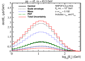
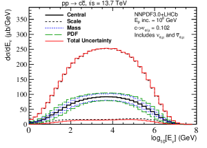
These differential cross-sections Eq. (16) have been computed in a range of values of $E$ and $E_{\nu}$ and then suitably interpolated. For each point in $\left(E;E_{\nu}\right)$, we have determined the relevant theoretical uncertainties from scales, PDFs, and $m_{c}$ variations. Our calculations use the improved NNPDF3.0+LHCb which includes the constraints from the 7 TeV charm data. A representative sample of our predictions are provided in Fig. 19, where we show the differential cross-section for the production of neutrinos from charm decay in $pp$ collisions, Eq. (16), as a function of the neutrino energy, computed with the POWHEG calculation. Results are shown for two values of the incoming cosmic ray energy, $E=10^{3}$ GeV (left plot) and $E=10^{8}$ GeV (right plot). We show the central prediction as well as the individual contributions from scale, PDF and $m_{c}$ uncertainties, as well as the overall theoretical uncertainty band computed from adding these uncertainties in quadrature. We see that at the highest energies, $E=10^{8}$ GeV, the total uncertainty band is dominated by scale variations, while PDF uncertainties are under control thanks to the constraints from the LHCb charm production data. We stress that while NLO QCD scale uncertainties are still large, up to a factor three, recent work towards the NNLO differential distributions for heavy quark production [56, 57] will provide a reduction of these higher-order uncertainties.

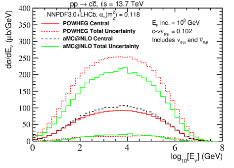
A powerful cross-check of the robustness of the predictions shown in Fig. 19 is provided by the fact that comparable results are obtained using either POWHEG or aMC@NLO, both for the central prediction and for the upper and lower ranges of the total theory uncertainty band, as shown in Fig. 20, when the same theory settings are used in the two calculations. Let us emphasise that two completely independent codes are used, with different underlying matrix element calculations and different matching to the parton showers, so this agreement is an indication of the robustness of the pQCD predictions for the charm-induced neutrino production cross-sections presented here.

Figure 20: Same as the right plot of Fig. 19, now comparing the predictions of POWHEG with those of aMC@NLO. The same theory settings are used in the two calculations. Only the central curve total theory uncertainty bands are shown for the predictions obtained with the two event generators.

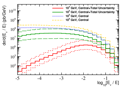
It is also interesting to study the dependence of our results for the charm-induced neutrino production cross-sections as a function of the incoming cosmic ray energy $E$. In Fig. 21 we represent the differential cross-section for neutrino production in charm decays, Eq. (16), for different values of $E$, as a function of the ratio between the neutrino energy $E_{\nu}$ and the cosmic ray energy, $z\equiv E_{\nu}/E_{p}$, that is,

$${{d\sigma(pN\to\nu X;E;E_{\nu}=zE)}\over{dz}}\,,\quad z={{E_{\nu}}\over{E}}\,,$$ (18)

which allows to compare the increase of the neutrino production cross-section, due to the larger value of $E$, for the same value of $z$, the ratio of the neutrino energy over the incoming cosmic ray energy. In Fig. 21 results are shown for $E=10^{3}$ and $E=10^{6}$ GeV (both central values and total theoretical uncertainty) and then for $E=10^{8}$ and $E=10^{9}$ GeV (only central values). Note how the cross-sections fall steeply as one approaches the kinematical boundary, $z\to 1$.

Figure 21: The dependence on the incoming cosmic ray energy $E$ of the prompt neutrino production cross-section $d\sigma/dE_{\nu}$, plotted as a function of $z\equiv E_{\nu}/E$, Eq. (18), which allows to compare calculations for different values of $E$. Results are shown for $E=10^{3}$ and $E=10^{6}$ GeV (both central values and total theoretical uncertainty) and then for $E=10^{8}$ and $E=10^{9}$ GeV (only central values). The cross-sections fall steeply as one approaches the kinematical boundary $z\to 1$.

Note that in pQCD, the correct expression for representing the dependence of $E$ of the prompt neutrino production cross-section is given by Eq. (18), shown in Fig. 21. Previous works, for example [13], present their calculations of the charm production cross-section as $d\sigma/dx_{c}$, where $x_{c}=E_{c}/E$, the ratio of produced charm quark energy over the incoming proton energy. However, the charm quark energy is only well defined at leading order, beyond which this is not true, and moreover is not accessible experimentally. Therefore, a robust comparison of theoretical calculations should always be presented at the level of the physical $D$ production cross-section. Alternatively, one might rescale by the charm branching fraction as in Eq. (11), but this approximation is only valid for relatively inclusive observables.

Finally, let us mention that our calculations for Eq. (16), illustrated in Figs. 19 and 20, are available for a wide range of $E$ and $E_{\nu}$ values in the format of interpolated tables that can be used as input for calculations of the prompt neutrino flux at IceCube, and are available from the authors upon request.

6 Summary and outlook

In this work we have performed a detailed study of charm and bottom production in the forward region, based on state-of-the-art pQCD with NLO calculations matched to parton showers. Our motivation was to provide a robust estimate of the theoretical uncertainties associated to the prompt neutrino flux at neutrino telescopes like IceCube, which is the dominant background for the detection of astrophysical neutrinos.

Our strategy was based on the careful validation of the pQCD calculations with the LHCb charm and bottom production data at 7 TeV, which cover the same kinematical region as that relevant for the production of prompt neutrinos at IceCube. We found that, with a suitable normalisation of the differential distributions, it is possible to include the 7 TeV $D$ meson data from LHCb in order to significantly constrain the poorly known small-$x$ gluon. Being able to include the LHCb charm measurements in a global NLO PDF fit further enhances our confidence of the applicability of pQCD to provide predictions for the prompt neutrino flux. These improved PDFs, NNPDF3.0+LHCb, which include the information from the LHCb charm data, are then used to construct the predictions for charm and bottom production at LHCb for the recently started Run II with a centre-of-mass energy of 13 TeV, as well as for the ratio of 13 over 7 TeV cross-sections.

Our main result for the cross-sections of the production of prompt neutrinos in charmed meson decays originating from cosmic ray collisions in the atmosphere is summarised in Figs. 19, 20 and 21. The main difference as compared to previous calculations of the prompt neutrino flux is that our approach has been fully validated with the recent LHCb differential measurements on charm production, and that the input PDF set used in our calculations is one that already includes the constraints from the LHCb charm data. We would like to emphasise that our calculations, both for the central values and for the various theoretical uncertainties, have been carefully benchmarked using three independent codes.

The main results of our study can be summarised as follows:

• pQCD predictions for charm and bottom production in the forward region are consistent with the recent LHCb 7 TeV measurements within theoretical uncertainties. Predictions obtained with three different codes, two Monte Carlo parton shower programs, aMC@NLO and POWHEG, and one semi-analytical calculation, FONLL, yield comparable results, both for the central value and for the total uncertainty.

• It is possible to include the LHCb charm data in the NNPDF3.0 NLO global analysis, achieving a substantial reduction of the PDF uncertainties on the poorly known small-$x$ gluon. In order to reduce the large scale uncertainties of the NLO calculation, the LHCb data have been normalised to a fixed reference bin.

• Run II of the LHC has just started, and the LHCb experiment will soon measure charm and bottom production in the forward region at 13 TeV, which will further explore the low-$x$ region of gluon PDF providing unique information on the structure of the proton. We have thus provided predictions for charm and bottom production at 13 TeV, as well as for the ratio of differential cross-sections between 13 and 7 TeV. These new measurements, both the 13 TeV (normalised) differential distributions and the 13 over 7 TeV cross-section ratio, offer new possibilities for PDF constraints, in particular thanks to the extended coverage at small-$x$ as compared to the 7 TeV measurements.

• Using the theory prediction for the ratio of inclusive fiducial cross-sections $R_{13/7}$ combined with the corresponding LHCb 7 TeV measurements, we are able to provide a prediction for the 13 TeV fiducial cross-section with substantially reduced uncertainties as that compared to the prediction from the NLO QCD calculation.

• We have provided QCD predictions for the differential cross-sections for the production of neutrinos from charm decay in $pA$ collisions, Eq. (16), using two independent NLO Monte Carlo generators, across a wide range of incoming cosmic ray energies $E$, and accounting for all relevant theory uncertainties.

It will be interesting to compare the upcoming 13 TeV LHCb measurements with the predictions presented in this paper. In particular, one should verify that the constraints on the small-$x$ gluon obtained from the inclusion on the PDF fit of the measurement of the ratio $R_{13/7}$ of differential distributions are consistent with those that have been obtained from the 7 TeV normalised charm production cross-sections. Likewise, comparing the inclusive fiducial cross-sections at 13 TeV with our predictions based on $R_{13/7}$ will be an important test of the validity of QCD calculations in this new kinematical region.

It is beyond the scope of this paper to explore quantitatively the implications of our calculations for the recent IceCube measurements of ultra high energy neutrinos. Our results for the charm-induced neutrino cross-sections as a function of $E$ and $E_{\nu}$ are available in the form of interpolated grids. This information can be used as input in a full calculation to derive robust predictions for the rates of prompt neutrino events expected at IceCube.

Appendix A Predictions for charm and bottom production at 13 TeV

In this appendix we provide a tabulation of our predictions for charm and bottom production in LHCb at TeV, presented in Sect. 4.1, as well as for the ratio of cross-sections between 13 TeV and 7 TeV, discussed in Sect. 4.2. For simplicity, we will restrict ourselves to the POWHEG results, since we have established from the comparison with aMC@NLO in Figs. 15 and 16 that the two calculations yield similar results.

A.1 Predictions for differential distributions at 13 TeV

First of all, in Table 3 we provide the predictions for the differential cross-sections for $D^{0}$ production at 13 TeV in the LHCb acceptance, corresponding to the results in Fig. 15. These results have been obtained with POWHEG using NNPDF3.0+LHCb as input PDF. For each bin, we provide the central value and the total theoretical uncertainty. To take into account the increased statistics that the Run II measurement will benefit from, we have used in this tabulation an optimised binning as compared to the 7 TeV results. First of all, we have used a finer binning at low $p_{T}$ (the region which is most sensitive to the gluon PDF) and extended our predictions up to $p_{T}^{D}=30$ GeV (where theoretical uncertainties are smallest). The corresponding predictions for any other choice of binning in $\left(p_{T}^{D},y^{D}\right)$ as well as for the other $D$ meson species are available from the authors upon request. As in the case of the 7 TeV results, absolute cross-sections are affected by substantial theoretical uncertainties, in particular due to the large scale variations of the NLO computation. On the other hand, PDF uncertainties are now subdominant for all values of $y^{D}$ and $p_{T}^{D}$, thanks for the constraints from the 7 TeV LHCb charm data.

${{d^{2}\sigma(D)(y,p_{T})}\over{dy^{D}dp_{T}^{D}}}\Delta y\,~{}(\mu b/{\rm GeV})$
$p_{T}^{D}$ (GeV)	$y^{D}$
	$2.0-2.5$			$2.5-3.0$			$3.0-3.5$			$3.5-4.0$			$4.0-4.5$
$0.0-0.25$	16.7		${}^{+41.4}_{-15.8}$	16.4		${}^{+40.6}_{-15.3}$	16.2		${}^{+41.0}_{-14.9}$	15.0		${}^{+38.0}_{-13.8}$	13.5		${}^{+34.0}_{-12.2}$
$0.25-0.5$	45.4		${}^{+109.8}_{-43.0}$	45.9		${}^{+114.6}_{-42.8}$	43.6		${}^{+108.7}_{-40.2}$	41.5		${}^{+103.5}_{-37.6}$	38.6		${}^{+96.4}_{-34.1}$
$0.5-0.75$	66.0		${}^{+156.6}_{-61.4}$	65.2		${}^{+157.6}_{-60.0}$	63.0		${}^{+153.0}_{-57.1}$	59.9		${}^{+146.3}_{-53.8}$	55.4		${}^{+136.1}_{-48.8}$
$0.75-1.0$	77.3		${}^{+178.6}_{-71.7}$	75.1		${}^{+174.6}_{-68.5}$	73.5		${}^{+171.5}_{-65.7}$	70.5		${}^{+167.5}_{-62.8}$	63.0		${}^{+148.6}_{-55.2}$
$1.0-1.25$	82.2		${}^{+181.7}_{-75.0}$	80.1		${}^{+178.5}_{-72.2}$	76.1		${}^{+171.0}_{-67.5}$	72.4		${}^{+164.2}_{-63.4}$	66.8		${}^{+152.9}_{-57.9}$
$1.25-1.5$	79.6		${}^{+168.0}_{-71.8}$	77.7		${}^{+165.2}_{-69.2}$	73.8		${}^{+155.5}_{-64.8}$	69.9		${}^{+150.3}_{-60.2}$	63.7		${}^{+138.2}_{-54.6}$
$1.5-1.75$	76.2		${}^{+152.2}_{-67.7}$	73.4		${}^{+148.8}_{-64.1}$	69.9		${}^{+143.0}_{-60.0}$	65.8		${}^{+137.1}_{-56.0}$	59.3		${}^{+124.0}_{-49.8}$
$1.75-2.0$	69.7		${}^{+132.7}_{-60.9}$	67.7		${}^{+129.5}_{-58.5}$	64.8		${}^{+127.6}_{-54.8}$	59.7		${}^{+117.2}_{-49.2}$	53.1		${}^{+106.5}_{-44.0}$
$2.0-2.25$	62.7		${}^{+112.3}_{-53.8}$	59.8		${}^{+108.0}_{-50.1}$	57.5		${}^{+107.0}_{-47.4}$	52.0		${}^{+97.1}_{-42.6}$	46.9		${}^{+89.1}_{-37.6}$
$2.25-2.5$	55.3		${}^{+95.1}_{-46.3}$	53.1		${}^{+91.5}_{-43.8}$	50.2		${}^{+88.4}_{-40.8}$	46.3		${}^{+82.2}_{-36.8}$	40.2		${}^{+72.6}_{-31.8}$
$2.5-2.75$	49.7		${}^{+82.8}_{-41.1}$	46.5		${}^{+77.1}_{-37.7}$	43.7		${}^{+73.2}_{-34.7}$	39.3		${}^{+67.2}_{-30.8}$	34.7		${}^{+58.8}_{-26.7}$
$2.75-3.0$	43.4		${}^{+68.7}_{-35.0}$	41.2		${}^{+66.2}_{-32.5}$	37.9		${}^{+60.6}_{-29.2}$	34.0		${}^{+56.2}_{-25.8}$	29.3		${}^{+49.2}_{-21.8}$
$3.0-3.5$	35.7		${}^{+53.6}_{-28.1}$	33.5		${}^{+50.6}_{-25.7}$	30.7		${}^{+46.8}_{-23.1}$	27.6		${}^{+42.6}_{-20.4}$	22.9		${}^{+35.9}_{-16.8}$
$3.5-4.0$	26.9		${}^{+37.5}_{-20.2}$	25.0		${}^{+34.8}_{-18.3}$	22.9		${}^{+32.4}_{-16.5}$	20.0		${}^{+28.8}_{-14.3}$	16.7		${}^{+24.5}_{-11.6}$
$4.0-4.5$	19.9		${}^{+26.0}_{-14.3}$	18.9		${}^{+25.0}_{-13.2}$	16.6		${}^{+21.6}_{-11.5}$	14.2		${}^{+18.7}_{-9.6}$	11.8		${}^{+15.9}_{-7.9}$
$4.5-5.0$	15.2		${}^{+19.0}_{-10.5}$	13.9		${}^{+17.3}_{-9.4}$	12.1		${}^{+15.3}_{-8.0}$	10.3		${}^{+13.0}_{-6.7}$	8.3		${}^{+10.9}_{-5.3}$
$5.0-6.0$	10.2		${}^{+11.7}_{-6.7}$	9.0		${}^{+10.3}_{-5.8}$	8.1		${}^{+9.3}_{-5.0}$	6.7		${}^{+8.0}_{-4.1}$	5.0		${}^{+6.0}_{-3.0}$
$6.0-7.0$	5.85		${}^{+6.02}_{-3.53}$	5.11		${}^{+5.41}_{-3.0}$	4.43		${}^{+4.62}_{-2.55}$	3.55		${}^{+3.91}_{-1.99}$	2.67		${}^{+2.88}_{-1.48}$
$7.0-8.0$	3.63		${}^{+3.41}_{-2.0}$	3.11		${}^{+3.02}_{-1.7}$	2.65		${}^{+2.61}_{-1.38}$	2.06		${}^{+2.0}_{-1.08}$	1.52		${}^{+1.55}_{-0.78}$
$8.0-9.0$	2.21		${}^{+1.98}_{-1.14}$	1.89		${}^{+1.68}_{-0.97}$	1.57		${}^{+1.42}_{-0.77}$	1.25		${}^{+1.2}_{-0.6}$	0.78		${}^{+0.74}_{-0.37}$
$9.0-10.0$	1.45		${}^{+1.23}_{-0.71}$	1.21		${}^{+1.05}_{-0.57}$	1.0		${}^{+0.87}_{-0.47}$	0.75		${}^{+0.67}_{-0.34}$	0.46		${}^{+0.41}_{-0.2}$
$10.0-15.0$	0.54		${}^{+0.42}_{-0.24}$	0.45		${}^{+0.35}_{-0.19}$	0.34		${}^{+0.26}_{-0.14}$	0.25		${}^{+0.2}_{-0.1}$	0.16		${}^{+0.12}_{-0.06}$
$15.0-20.0$	0.12		${}^{+0.08}_{-0.04}$	0.1		${}^{+0.07}_{-0.04}$	0.07		${}^{+0.05}_{-0.03}$	0.04		${}^{+0.03}_{-0.01}$	0.02		${}^{+0.02}_{-0.01}$
$20.0-30.0$	0.029		${}^{+0.018}_{-0.008}$	0.025		${}^{+0.014}_{-0.008}$	0.016		${}^{+0.009}_{-0.005}$	0.009		${}^{+0.006}_{-0.003}$	0.003		${}^{+0.002}_{-0.001}$

Table 3: Predictions for the differential cross-sections for $D^{0}$ meson production at LHCb at 13 TeV, computed using POWHEG and NNPDF3.0+LHCb. For each bin we indicate the central value and the total theoretical uncertainty. Predictions for different binnings and for other $D$ meson species are available upon request.

The corresponding predictions for the differential cross-sections of the production of $B^{0}$ mesons at LHCb Run II are shown in Table 4, which is the analog of Table 3 for charm production. These predictions were represented graphically (and compared to the aMC@NLO calculation) in Fig. 16. In this case we have assumed the same binning as in the 7 TeV measurement. As compared to the 13 TeV charm predictions, the higher scales and the larger values of Bjorken-$x$ probed in the case of bottom production result in reduced theory uncertainties. The total uncertainty is around $50\%$, with differences depending on the specific bin, and is again dominated by scale uncertainties.

${{d^{2}\sigma(B)(y,p_{T})}\over{dy^{B}dp_{T}^{B}}}(\mu b/{\rm GeV})$
$p_{T}^{B}$ (GeV)	$y^{B}$
	$2.0-2.5$			$2.5-3.0$			$3.0-3.5$			$3.5-4.0$			$4.0-4.5$
$0.0-0.5$	0.6		${}^{+0.37}_{-0.28}$	0.53		${}^{+0.34}_{-0.25}$	0.45		${}^{+0.29}_{-0.21}$	0.4		${}^{+0.25}_{-0.18}$	0.32		${}^{+0.2}_{-0.13}$
$0.5-1.0$	1.67		${}^{+1.0}_{-0.8}$	1.53		${}^{+0.94}_{-0.73}$	1.36		${}^{+0.84}_{-0.62}$	1.14		${}^{+0.71}_{-0.51}$	0.91		${}^{+0.56}_{-0.4}$
$1.0-1.5$	2.56		${}^{+1.58}_{-1.21}$	2.32		${}^{+1.42}_{-1.07}$	2.05		${}^{+1.27}_{-0.93}$	1.75		${}^{+1.07}_{-0.77}$	1.39		${}^{+0.83}_{-0.59}$
$1.5-2.0$	3.27		${}^{+1.98}_{-1.54}$	2.96		${}^{+1.77}_{-1.36}$	2.58		${}^{+1.57}_{-1.15}$	2.21		${}^{+1.33}_{-0.97}$	1.77		${}^{+1.07}_{-0.76}$
$2.0-2.5$	3.68		${}^{+2.19}_{-1.68}$	3.34		${}^{+1.99}_{-1.49}$	2.93		${}^{+1.76}_{-1.29}$	2.45		${}^{+1.46}_{-1.04}$	1.98		${}^{+1.18}_{-0.83}$
$2.5-3.0$	3.91		${}^{+2.3}_{-1.76}$	3.55		${}^{+2.09}_{-1.57}$	3.1		${}^{+1.82}_{-1.33}$	2.58		${}^{+1.52}_{-1.07}$	2.05		${}^{+1.2}_{-0.84}$
$3.0-3.5$	3.99		${}^{+2.25}_{-1.76}$	3.58		${}^{+2.06}_{-1.53}$	3.16		${}^{+1.82}_{-1.32}$	2.64		${}^{+1.51}_{-1.09}$	2.04		${}^{+1.16}_{-0.82}$
$3.5-4.0$	3.91		${}^{+2.17}_{-1.68}$	3.49		${}^{+1.96}_{-1.46}$	3.06		${}^{+1.7}_{-1.25}$	2.54		${}^{+1.44}_{-1.01}$	1.97		${}^{+1.11}_{-0.76}$
$4.0-4.5$	3.71		${}^{+2.03}_{-1.54}$	3.36		${}^{+1.83}_{-1.37}$	2.9		${}^{+1.6}_{-1.17}$	2.4		${}^{+1.3}_{-0.93}$	1.82		${}^{+0.98}_{-0.67}$
$4.5-5.0$	3.5		${}^{+1.87}_{-1.43}$	3.16		${}^{+1.68}_{-1.27}$	2.67		${}^{+1.42}_{-1.04}$	2.21		${}^{+1.18}_{-0.84}$	1.69		${}^{+0.91}_{-0.62}$
$5.0-5.5$	3.17		${}^{+1.69}_{-1.25}$	2.87		${}^{+1.49}_{-1.12}$	2.43		${}^{+1.27}_{-0.91}$	1.98		${}^{+1.05}_{-0.72}$	1.5		${}^{+0.77}_{-0.53}$
$5.5-6.0$	2.89		${}^{+1.48}_{-1.12}$	2.6		${}^{+1.31}_{-0.98}$	2.22		${}^{+1.13}_{-0.82}$	1.77		${}^{+0.89}_{-0.62}$	1.34		${}^{+0.68}_{-0.46}$
$6.0-6.5$	2.63		${}^{+1.29}_{-1.0}$	2.33		${}^{+1.15}_{-0.87}$	1.97		${}^{+0.97}_{-0.69}$	1.58		${}^{+0.76}_{-0.55}$	1.15		${}^{+0.57}_{-0.37}$
$6.5-7.0$	2.36		${}^{+1.14}_{-0.87}$	2.05		${}^{+1.0}_{-0.73}$	1.74		${}^{+0.85}_{-0.61}$	1.38		${}^{+0.67}_{-0.45}$	0.98		${}^{+0.48}_{-0.31}$
$7.0-7.5$	2.07		${}^{+0.99}_{-0.74}$	1.84		${}^{+0.88}_{-0.65}$	1.52		${}^{+0.73}_{-0.5}$	1.2		${}^{+0.56}_{-0.38}$	0.86		${}^{+0.41}_{-0.27}$
$7.5-8.0$	1.82		${}^{+0.87}_{-0.63}$	1.61		${}^{+0.76}_{-0.54}$	1.33		${}^{+0.62}_{-0.43}$	1.04		${}^{+0.47}_{-0.32}$	0.72		${}^{+0.34}_{-0.22}$
$8.0-8.5$	1.62		${}^{+0.74}_{-0.55}$	1.41		${}^{+0.65}_{-0.47}$	1.15		${}^{+0.51}_{-0.36}$	0.88		${}^{+0.39}_{-0.26}$	0.62		${}^{+0.28}_{-0.18}$
$8.5-9.0$	1.41		${}^{+0.63}_{-0.46}$	1.23		${}^{+0.55}_{-0.39}$	1.01		${}^{+0.45}_{-0.31}$	0.77		${}^{+0.35}_{-0.23}$	0.52		${}^{+0.24}_{-0.14}$
$9.0-9.5$	1.22		${}^{+0.55}_{-0.39}$	1.07		${}^{+0.48}_{-0.33}$	0.87		${}^{+0.38}_{-0.26}$	0.66		${}^{+0.29}_{-0.19}$	0.45		${}^{+0.2}_{-0.12}$
$9.5-10.0$	1.11		${}^{+0.48}_{-0.35}$	0.93		${}^{+0.4}_{-0.28}$	0.77		${}^{+0.33}_{-0.23}$	0.58		${}^{+0.26}_{-0.16}$	0.39		${}^{+0.16}_{-0.11}$
$10.0-10.5$	0.95		${}^{+0.41}_{-0.29}$	0.82		${}^{+0.35}_{-0.24}$	0.66		${}^{+0.28}_{-0.19}$	0.48		${}^{+0.21}_{-0.12}$	0.33		${}^{+0.14}_{-0.09}$
$10.5-11.5$	0.79		${}^{+0.33}_{-0.23}$	0.67		${}^{+0.28}_{-0.19}$	0.53		${}^{+0.22}_{-0.14}$	0.4		${}^{+0.16}_{-0.1}$	0.26		${}^{+0.11}_{-0.07}$
$11.5-12.5$	0.61		${}^{+0.25}_{-0.17}$	0.51		${}^{+0.21}_{-0.14}$	0.4		${}^{+0.17}_{-0.1}$	0.3		${}^{+0.12}_{-0.08}$	0.18		${}^{+0.07}_{-0.05}$
$12.5-14.0$	0.45		${}^{+0.18}_{-0.12}$	0.38		${}^{+0.15}_{-0.1}$	0.29		${}^{+0.12}_{-0.08}$	0.21		${}^{+0.08}_{-0.05}$	0.13		${}^{+0.05}_{-0.03}$
$14.0-16.5$	0.28		${}^{+0.11}_{-0.07}$	0.23		${}^{+0.09}_{-0.06}$	0.18		${}^{+0.07}_{-0.04}$	0.12		${}^{+0.05}_{-0.03}$	0.07		${}^{+0.03}_{-0.02}$
$16.5-23.5$	0.11		${}^{+0.04}_{-0.03}$	0.09		${}^{+0.03}_{-0.02}$	0.06		${}^{+0.02}_{-0.01}$	0.04		${}^{+0.01}_{-0.01}$	0.02		${}^{+0.01}_{-0.0}$
$23.5-40.0$	0.019		${}^{+0.006}_{-0.004}$	0.014		${}^{+0.005}_{-0.003}$	0.01		${}^{+0.003}_{-0.002}$	0.005		${}^{+0.002}_{-0.001}$	0.002		${}^{+0.001}_{-0.001}$

Table 4: Same as Table 3, now for the production of $B^{0}$ mesons at 13 TeV. Predictions for different binnings and for other $B$ mesons are available upon request.

A.2 Predictions for the ratio $R_{13/7}$

Next we turn to the predictions for the ratio $R_{13/7}$ of the differential distributions for heavy quark production at LHCb between 13 TeV and 7 TeV, Eqns. (4) and (5), discussed in Sect. 4.2. In Table 5 we show the ratio $R_{13/7}$ for $D^{0}$ mesons using POWHEG and NNPDF3.0+LHCb. These predictions were represented graphically in Fig. 17. We provide the central value of $R_{13/7}$ and the total theoretical uncertainty, which as can be seen from Fig. 17 arises predominantly due to scale variations. When evaluating Eq. (4), scale variations, charm mass variations and PDF variations are considered to be fully correlated between 13 and 7 TeV.

$R_{13/7}^{D}={{d^{2}\sigma(D)(y,p_{T},13~{}{\rm TeV})}\over{dy^{D}dp_{T}^{D}}}\Big{/}{{d^{2}\sigma(D)(y,p_{T},7~{}{\rm TeV})}\over{dy^{D}dp_{T}^{D}}}$
$p_{T}^{D}$ (GeV)	$y^{D}$
	$2.0-2.5$			$2.5-3.0$			$3.0-3.5$			$3.5-4.0$			$4.0-4.5$
$0.0-1.0$	1.23		${}^{+0.13}_{-0.35}$	1.25		${}^{+0.13}_{-0.35}$	1.28		${}^{+0.15}_{-0.32}$	1.33		${}^{+0.15}_{-0.32}$	1.38		${}^{+0.17}_{-0.27}$
$1.0-2.0$	1.26		${}^{+0.12}_{-0.34}$	1.29		${}^{+0.12}_{-0.37}$	1.32		${}^{+0.13}_{-0.35}$	1.38		${}^{+0.13}_{-0.31}$	1.46		${}^{+0.14}_{-0.31}$
$2.0-3.0$	1.31		${}^{+0.11}_{-0.31}$	1.33		${}^{+0.12}_{-0.29}$	1.39		${}^{+0.12}_{-0.31}$	1.45		${}^{+0.13}_{-0.33}$	1.57		${}^{+0.15}_{-0.3}$
$3.0-4.0$	1.39		${}^{+0.1}_{-0.26}$	1.43		${}^{+0.11}_{-0.26}$	1.5		${}^{+0.11}_{-0.27}$	1.61		${}^{+0.13}_{-0.33}$	1.72		${}^{+0.16}_{-0.32}$
$4.0-5.0$	1.49		${}^{+0.1}_{-0.22}$	1.53		${}^{+0.13}_{-0.24}$	1.61		${}^{+0.12}_{-0.26}$	1.72		${}^{+0.14}_{-0.29}$	2.01		${}^{+0.16}_{-0.39}$
$5.0-6.0$	1.57		${}^{+0.11}_{-0.24}$	1.65		${}^{+0.12}_{-0.25}$	1.79		${}^{+0.11}_{-0.26}$	1.99		${}^{+0.11}_{-0.25}$	2.18		${}^{+0.19}_{-0.35}$
$6.0-7.0$	1.67		${}^{+0.13}_{-0.24}$	1.75		${}^{+0.12}_{-0.23}$	1.85		${}^{+0.14}_{-0.28}$	1.98		${}^{+0.21}_{-0.27}$
$7.0-8.0$	1.78		${}^{+0.1}_{-0.18}$	1.84		${}^{+0.09}_{-0.18}$	2.02		${}^{+0.12}_{-0.15}$	2.17		${}^{+0.16}_{-0.31}$

Table 5: Predictions for the ratio $R_{13/7}^{D}$ of double differential cross-sections for $D^{0}$ meson production between 13 and 7 TeV at LHCb, Eq. (4) Results have obtained using POWHEG with the NNPDF3.0+LHCb NLO PDF set. The same binning as in the 7 TeV measurement is assumed at 13 TeV. In each bin, we provide the central prediction and the total theoretical uncertainty, obtained from the sum in quadrature of scales, PDFs and charm mass variations. See Fig. 17 for the graphical representation of these predictions.

In order to evaluate the impact of the reduction of PDF uncertainties on the observable $R^{D}_{13/7}$, that has been achieved by including in NNPDF3.0 the LHCb 7 TeV charm production data, it is useful to compare with the corresponding predictions with the original NNPDF3.0 set. With this motivation, in Table 6 we show ratio $R_{13/7}({\rm orig})$ computed with the original NNPDF3.0 PDF set, which should be compared with the predictions obtained with the NNPDF3.0+LHCb set in Table 5. The data is ordered in increasing rapidity bins, and within each of these in increasing $p_{T}$ bins. For each bin, we show the central prediction, the PDF uncertainty and the the total theory uncertainty for $R^{D}_{13/7}({\rm orig})$, as well as the ratio between the predictions for the ratio itself computed with NNPDF3.0+LHCb and with the original NNPDF3.0, $R^{D}_{13/7}({\rm new})/R^{D}_{13/7}({\rm orig})$.

From the comparison between Tables 6 and 5 we see first of all that the predictions for the central value of $R^{D}_{13/7}$ are reasonably stable: differences for the central value computed between the original and new PDFs are typically a few percent, rather smaller than the total theory uncertainties. This nicely illustrates the compatibility of the NNPDF3.0 small-$x$ gluon with the 7 TeV LHCb charm production data. The real difference comes from the reduction in PDF uncertainties: since scale and charm mass uncertainties are essentially the same in $R^{D}_{13/7}({\rm new})$ and $R^{D}_{13/7}({\rm old})$, the differences between the total theory errors stem from the reduction of PDF uncertainties in $R_{13/7}({\rm new})$. For instance, in the lowest $p_{T}$ and most forward region (data bin 33), the relative total theory uncertainty of $R^{D}_{13/7}({\rm orig})$ is $~{}^{+30\%}_{-38\%}$, while for $R^{D}_{13/7}({\rm new})$ the corresponding uncertainty is substantially reduced reduced down to $~{}^{+17\%}_{-27\%}$. Similar comparisons can be performed for other bins.

Data Index	$R_{13/7}({\rm new})$/$R_{13/7}({\rm orig})$	$R_{13/7}({\rm orig})$ cv	$R_{13/7}({\rm orig})$ PDF	$R_{13/7}({\rm orig})$ Tot
1	0.9	1.36	$\pm$0.19	${}^{+0.23}_{-0.43}$
2	0.93	1.35	$\pm$0.18	${}^{+0.22}_{-0.4}$
3	0.94	1.39	$\pm$0.19	${}^{+0.21}_{-0.37}$
4	0.95	1.47	$\pm$0.18	${}^{+0.2}_{-0.32}$
5	0.97	1.55	$\pm$0.15	${}^{+0.18}_{-0.27}$
6	0.99	1.59	$\pm$0.13	${}^{+0.17}_{-0.27}$
7	1.0	1.67	$\pm$0.12	${}^{+0.18}_{-0.27}$
8	1.01	1.75	$\pm$0.09	${}^{+0.13}_{-0.2}$
9	0.88	1.42	$\pm$0.19	${}^{+0.23}_{-0.43}$
10	0.92	1.41	$\pm$0.17	${}^{+0.21}_{-0.44}$
11	0.93	1.42	$\pm$0.17	${}^{+0.2}_{-0.35}$
12	0.96	1.5	$\pm$0.16	${}^{+0.19}_{-0.31}$
13	0.96	1.6	$\pm$0.15	${}^{+0.2}_{-0.29}$
14	0.95	1.73	$\pm$0.18	${}^{+0.22}_{-0.31}$
15	0.96	1.81	$\pm$0.16	${}^{+0.2}_{-0.29}$
16	0.99	1.85	$\pm$0.14	${}^{+0.16}_{-0.22}$
17	0.88	1.46	$\pm$0.2	${}^{+0.25}_{-0.4}$
18	0.91	1.44	$\pm$0.18	${}^{+0.22}_{-0.42}$
19	0.93	1.48	$\pm$0.16	${}^{+0.2}_{-0.36}$
20	0.95	1.58	$\pm$0.14	${}^{+0.18}_{-0.32}$
21	0.95	1.69	$\pm$0.15	${}^{+0.19}_{-0.3}$
22	1.02	1.75	$\pm$0.16	${}^{+0.19}_{-0.3}$
23	1.0	1.85	$\pm$0.16	${}^{+0.21}_{-0.32}$
24	1.02	1.97	$\pm$0.17	${}^{+0.19}_{-0.21}$
25	0.88	1.51	$\pm$0.25	${}^{+0.29}_{-0.43}$
26	0.91	1.51	$\pm$0.19	${}^{+0.23}_{-0.38}$
27	0.92	1.57	$\pm$0.16	${}^{+0.21}_{-0.39}$
28	0.96	1.68	$\pm$0.15	${}^{+0.2}_{-0.37}$
29	0.97	1.78	$\pm$0.15	${}^{+0.2}_{-0.33}$
30	1.01	1.98	$\pm$0.16	${}^{+0.18}_{-0.29}$
31	0.95	2.09	$\pm$0.17	${}^{+0.27}_{-0.32}$
32	1.04	2.09	$\pm$0.16	${}^{+0.21}_{-0.33}$
33	0.86	1.61	$\pm$0.24	${}^{+0.3}_{-0.38}$
34	0.9	1.61	$\pm$0.21	${}^{+0.25}_{-0.39}$
35	0.92	1.7	$\pm$0.18	${}^{+0.23}_{-0.36}$
36	0.93	1.85	$\pm$0.17	${}^{+0.23}_{-0.37}$
37	0.98	2.04	$\pm$0.16	${}^{+0.22}_{-0.42}$
38	0.99	2.21	$\pm$0.2	${}^{+0.27}_{-0.4}$

Table 6: The ratio $R_{13/7}$ computed with the original NNPDF3.0 PDF set, in order to compare with the predictions obtained with the NNPDF3.0+LHCb set in Table 5. The data is ordered in increasing rapidity bins, an within each of these, in increasing $p_{T}$ bins. For each bin, we show the central prediction, the PDF uncertainty and the the total theory uncertainty for $R_{13/7}({\rm orig})$, as well as the ratio between the new and orig predictions for the ratio itself, $R_{13/7}({\rm new})/R_{13/7}({\rm orig})$.

We should mention that, once a measurement of $R_{13/7}$ becomes available, it should be possible to include this data in a global PDF fit in a similar way as we have done with the 7 TeV charm normalised cross-sections. One expects similar improvements in the low-$x$ gluon, though perhaps the increased lever arm in $x$ of the 13 TeV data will increase the constraining power towards smaller values of $x$. As discussed in Sect. 4.2, the main advantage of the ratio measurement is the cancellation of theory systematics, in particular from scale variations.

We have also computed the value of ratio of inclusive fiducial cross-sections, as explained in Sect. 4.3, but this time for original NNPDF3.0 set, which turns out to be

$$R_{D}({\rm orig})=1.52\,^{+0.19\,(12.6\%)}_{-0.34\,(22.6\%)}\,,$$ (19)

where we provide the total theoretical uncertainty of the prediction. This should be compared with the result obtained with the NNPDF3.0+LHCb set, Eq. (8). The reduction of the total theory uncertainty in Eq. (8) as compared to Eq. (19) is a consequence of the constraints from the 7 TeV LHCb charm measurements.

We now provide the differential predictions for $B$ meson production at LHC Run II in LHCb. First of all, in Table 7 we provide the predictions for the ratio of double differential cross-sections for the production of $B^{0}$ mesons between 13 TeV and 7 TeV, see Eq. (5). These results were represented graphically in Fig. 16. This is the analog table as that for charm production in Table 5. As in the case of charm, we have assumed the same binning in $\left(p_{T}^{B},y^{B}\right)$ than the corresponding 7 TeV measurement. The magnitude of $R_{13/7}^{B}$ increases rapidly with increasing $p_{T}^{B}$ and $y^{B}$, where the 7 TeV cross-sections are close to their kinematical boundaries.

$R_{13/7}^{B}={{d^{2}\sigma(B)(y,p_{T},13~{}{\rm TeV})}\over{dy^{B}dp_{T}^{B}}}\Big{/}{{d^{2}\sigma(B)(y,p_{T},7~{}{\rm TeV})}\over{dy^{B}dp_{T}^{B}}}$
$p_{T}^{B}$ (GeV)	$y^{B}$
	$2.0-2.5$			$2.5-3.0$			$3.0-3.5$			$3.5-4.0$			$4.0-4.5$
$0.0-0.5$	1.56		${}^{+0.07}_{-0.11}$	1.6		${}^{+0.08}_{-0.13}$	1.59		${}^{+0.12}_{-0.14}$	1.77		${}^{+0.08}_{-0.17}$	1.85		${}^{+0.25}_{-0.17}$
$0.5-1.0$	1.54		${}^{+0.08}_{-0.14}$	1.6		${}^{+0.07}_{-0.15}$	1.66		${}^{+0.07}_{-0.15}$	1.74		${}^{+0.11}_{-0.15}$	1.93		${}^{+0.11}_{-0.16}$
$1.0-1.5$	1.53		${}^{+0.07}_{-0.13}$	1.59		${}^{+0.07}_{-0.15}$	1.65		${}^{+0.09}_{-0.15}$	1.75		${}^{+0.1}_{-0.15}$	1.95		${}^{+0.1}_{-0.14}$
$1.5-2.0$	1.55		${}^{+0.06}_{-0.13}$	1.59		${}^{+0.08}_{-0.13}$	1.66		${}^{+0.08}_{-0.14}$	1.8		${}^{+0.08}_{-0.14}$	1.99		${}^{+0.09}_{-0.2}$
$2.0-2.5$	1.53		${}^{+0.07}_{-0.13}$	1.58		${}^{+0.08}_{-0.14}$	1.66		${}^{+0.07}_{-0.13}$	1.78		${}^{+0.1}_{-0.16}$	2.01		${}^{+0.09}_{-0.18}$
$2.5-3.0$	1.55		${}^{+0.08}_{-0.13}$	1.62		${}^{+0.07}_{-0.13}$	1.69		${}^{+0.08}_{-0.14}$	1.79		${}^{+0.11}_{-0.15}$	1.98		${}^{+0.13}_{-0.17}$
$3.0-3.5$	1.58		${}^{+0.07}_{-0.13}$	1.62		${}^{+0.08}_{-0.14}$	1.71		${}^{+0.07}_{-0.14}$	1.87		${}^{+0.08}_{-0.16}$	2.03		${}^{+0.11}_{-0.17}$
$3.5-4.0$	1.59		${}^{+0.07}_{-0.13}$	1.65		${}^{+0.07}_{-0.14}$	1.73		${}^{+0.09}_{-0.15}$	1.89		${}^{+0.08}_{-0.13}$	2.09		${}^{+0.11}_{-0.18}$
$4.0-4.5$	1.58		${}^{+0.08}_{-0.13}$	1.67		${}^{+0.07}_{-0.14}$	1.76		${}^{+0.09}_{-0.15}$	1.95		${}^{+0.08}_{-0.17}$	2.15		${}^{+0.12}_{-0.17}$
$4.5-5.0$	1.63		${}^{+0.07}_{-0.13}$	1.71		${}^{+0.07}_{-0.15}$	1.77		${}^{+0.09}_{-0.15}$	1.96		${}^{+0.09}_{-0.17}$	2.26		${}^{+0.1}_{-0.19}$
$5.0-5.5$	1.62		${}^{+0.07}_{-0.13}$	1.71		${}^{+0.08}_{-0.14}$	1.81		${}^{+0.08}_{-0.14}$	2.01		${}^{+0.09}_{-0.16}$	2.27		${}^{+0.11}_{-0.16}$
$5.5-6.0$	1.65		${}^{+0.08}_{-0.14}$	1.73		${}^{+0.07}_{-0.13}$	1.88		${}^{+0.07}_{-0.15}$	2.06		${}^{+0.12}_{-0.2}$	2.39		${}^{+0.1}_{-0.2}$
$6.0-6.5$	1.69		${}^{+0.08}_{-0.15}$	1.78		${}^{+0.07}_{-0.15}$	1.89		${}^{+0.08}_{-0.15}$	2.11		${}^{+0.1}_{-0.2}$	2.42		${}^{+0.11}_{-0.17}$
$6.5-7.0$	1.73		${}^{+0.08}_{-0.15}$	1.76		${}^{+0.08}_{-0.14}$	1.92		${}^{+0.09}_{-0.15}$	2.15		${}^{+0.1}_{-0.18}$	2.44		${}^{+0.15}_{-0.19}$
$7.0-7.5$	1.74		${}^{+0.07}_{-0.14}$	1.87		${}^{+0.08}_{-0.16}$	1.95		${}^{+0.1}_{-0.15}$	2.23		${}^{+0.08}_{-0.17}$	2.54		${}^{+0.22}_{-0.21}$
$7.5-8.0$	1.76		${}^{+0.07}_{-0.13}$	1.85		${}^{+0.08}_{-0.15}$	1.97		${}^{+0.1}_{-0.14}$	2.24		${}^{+0.1}_{-0.17}$	2.53		${}^{+0.19}_{-0.2}$
$8.0-8.5$	1.81		${}^{+0.08}_{-0.13}$	1.93		${}^{+0.08}_{-0.16}$	2.03		${}^{+0.09}_{-0.15}$	2.26		${}^{+0.14}_{-0.18}$	2.75		${}^{+0.14}_{-0.19}$
$8.5-9.0$	1.8		${}^{+0.1}_{-0.13}$	1.9		${}^{+0.07}_{-0.13}$	2.1		${}^{+0.1}_{-0.16}$	2.33		${}^{+0.11}_{-0.17}$	2.78		${}^{+0.16}_{-0.19}$
$9.0-9.5$	1.83		${}^{+0.09}_{-0.12}$	1.98		${}^{+0.07}_{-0.16}$	2.1		${}^{+0.1}_{-0.17}$	2.42		${}^{+0.1}_{-0.19}$	2.82		${}^{+0.16}_{-0.18}$
$9.5-10.0$	1.89		${}^{+0.07}_{-0.14}$	1.96		${}^{+0.09}_{-0.15}$	2.11		${}^{+0.11}_{-0.16}$	2.49		${}^{+0.15}_{-0.21}$	3.01		${}^{+0.15}_{-0.24}$
$10.0-10.5$	1.88		${}^{+0.07}_{-0.13}$	2.02		${}^{+0.07}_{-0.16}$	2.2		${}^{+0.09}_{-0.17}$	2.41		${}^{+0.17}_{-0.15}$	3.09		${}^{+0.17}_{-0.21}$
$10.5-11.5$	1.94		${}^{+0.07}_{-0.14}$	2.05		${}^{+0.08}_{-0.13}$	2.19		${}^{+0.15}_{-0.16}$	2.59		${}^{+0.12}_{-0.14}$	3.31		${}^{+0.14}_{-0.32}$
$11.5-12.5$	1.94		${}^{+0.08}_{-0.13}$	2.07		${}^{+0.08}_{-0.14}$	2.3		${}^{+0.1}_{-0.17}$	2.78		${}^{+0.11}_{-0.22}$	3.32		${}^{+0.15}_{-0.21}$
$12.5-14.0$	2.03		${}^{+0.08}_{-0.14}$	2.15		${}^{+0.08}_{-0.14}$	2.48		${}^{+0.08}_{-0.19}$	2.88		${}^{+0.1}_{-0.23}$	3.72		${}^{+0.18}_{-0.28}$
$14.0-16.5$	2.11		${}^{+0.09}_{-0.14}$	2.27		${}^{+0.09}_{-0.15}$	2.6		${}^{+0.1}_{-0.2}$	3.06		${}^{+0.11}_{-0.2}$	4.12		${}^{+0.21}_{-0.22}$
$16.5-23.5$	2.24		${}^{+0.08}_{-0.13}$	2.42		${}^{+0.11}_{-0.14}$	2.86		${}^{+0.13}_{-0.17}$	3.47		${}^{+0.16}_{-0.22}$	4.77		${}^{+0.27}_{-0.44}$
$23.5-40.0$	2.6		${}^{+0.09}_{-0.14}$	2.88		${}^{+0.11}_{-0.13}$	3.6		${}^{+0.15}_{-0.23}$	4.81		${}^{+0.21}_{-0.39}$	7.45		${}^{+1.21}_{-0.59}$

Table 7: Same as Table 5 for the ratio $R_{13/7}^{B}$ of double differential cross-sections for $B^{0}$ mesons between 13 TeV and 7 TeV.

References

- [1] IceCube Collaboration, M. Aartsen et al., First observation of PeV-energy neutrinos with IceCube, Phys.Rev.Lett. 111 (2013) 021103, [arXiv:1304.5356].
- [2] IceCube Collaboration, M. Aartsen et al., Evidence for High-Energy Extraterrestrial Neutrinos at the IceCube Detector, Science 342 (2013) 1242856, [arXiv:1311.5238].
- [3] IceCube Collaboration, M. Aartsen et al., Observation of High-Energy Astrophysical Neutrinos in Three Years of IceCube Data, Phys.Rev.Lett. 113 (2014) 101101, [arXiv:1405.5303].
- [4] G. Barr, T. Gaisser, P. Lipari, S. Robbins, and T. Stanev, A Three - dimensional calculation of atmospheric neutrinos, Phys.Rev. D70 (2004) 023006, [astro-ph/0403630].
- [5] M. C. Gonzalez-Garcia, M. Maltoni, and J. Rojo, Determination of the atmospheric neutrino fluxes from atmospheric neutrino data, JHEP 10 (2006) 075, [hep-ph/0607324].
- [6] M. Honda, T. Kajita, K. Kasahara, S. Midorikawa, and T. Sanuki, Calculation of atmospheric neutrino flux using the interaction model calibrated with atmospheric muon data, Phys.Rev. D75 (2007) 043006, [astro-ph/0611418].
- [7] P. Lipari, Lepton spectra in the earth’s atmosphere, Astropart.Phys. 1 (1993) 195–227.
- [8] L. Pasquali, M. Reno, and I. Sarcevic, Lepton fluxes from atmospheric charm, Phys.Rev. D59 (1999) 034020, [hep-ph/9806428].
- [9] R. Enberg, M. H. Reno, and I. Sarcevic, Prompt neutrino fluxes from atmospheric charm, Phys.Rev. D78 (2008) 043005, [arXiv:0806.0418].
- [10] P. Gondolo, G. Ingelman, and M. Thunman, Charm production and high-energy atmospheric muon and neutrino fluxes, Astropart.Phys. 5 (1996) 309–332, [hep-ph/9505417].
- [11] A. Martin, M. Ryskin, and A. Stasto, Prompt neutrinos from atmospheric and production and the gluon at very small x, Acta Phys.Polon. B34 (2003) 3273–3304, [hep-ph/0302140].
- [12] G. Gelmini, P. Gondolo, and G. Varieschi, Prompt atmospheric neutrinos and muons: NLO versus LO QCD predictions, Phys.Rev. D61 (2000) 036005, [hep-ph/9904457].
- [13] A. Bhattacharya, R. Enberg, M. H. Reno, I. Sarcevic, and A. Stasto, Perturbative charm production and the prompt atmospheric neutrino flux in light of RHIC and LHC, arXiv:1502.01076.
- [14] M. V. Garzelli, S. Moch and G. Sigl, Lepton fluxes from atmospheric charm revisited, arXiv:1507.01570.
- [15] F. Riehn, R. Engel, A. Fedynitch, T. K. Gaisser, and T. Stanev, Charm production in SIBYLL, arXiv:1502.06353.
- [16] C. A. Arguelles, F. Halzen, L. Will, M. Kroll, and M. H. Reno, The High-Energy Behavior of Photon, Neutrino and Proton Cross Sections, arXiv:1504.06639.
- [17] G. Watt, Parton distribution function dependence of benchmark Standard Model total cross sections at the 7 TeV LHC, JHEP 1109 (2011) 069, [arXiv:1106.5788].
- [18] J. Rojo et al., The PDF4LHC report on PDFs and LHC data: Results from Run I and preparation for Run II, arXiv:1507.00556.
- [19] R. D. Ball, S. Carrazza, L. Del Debbio, S. Forte, J. Gao, et al., Parton Distribution Benchmarking with LHC Data, JHEP 1304 (2013) 125, [arXiv:1211.5142].
- [20] J. Gao, M. Guzzi, J. Huston, H.-L. Lai, Z. Li, et al., The CT10 NNLO Global Analysis of QCD, arXiv:1302.6246.
- [21] The NNPDF Collaboration, R. D. Ball et al., A first unbiased global NLO determination of parton distributions and their uncertainties, Nucl. Phys. B838 (2010) 136–206, [arXiv:1002.4407].
- [22] L. Harland-Lang, A. Martin, P. Motylinski, and R. Thorne, Parton distributions in the LHC era: MMHT 2014 PDFs, Eur.Phys.J. C75 (2015), no. 5 204, [arXiv:1412.3989].
- [23] R. Ball and R. K. Ellis, Heavy quark production at high-energy, JHEP 0105 (2001) 053, [hep-ph/0101199].
- [24] G. Altarelli, R. D. Ball, and S. Forte, Small x Resummation with Quarks: Deep-Inelastic Scattering, Nucl. Phys. B799 (2008) 199–240, [arXiv:0802.0032].
- [25] M. Ciafaloni, D. Colferai, G. Salam, and A. Stasto, A Matrix formulation for small-x singlet evolution, JHEP 0708 (2007) 046, [arXiv:0707.1453].
- [26] H1 and ZEUS Collaboration, F. Aaron et al., Combined Measurement and QCD Analysis of the Inclusive Scattering Cross Sections at HERA, JHEP 1001 (2010) 109, [arXiv:0911.0884].
- [27] F. Caola, S. Forte, and J. Rojo, Deviations from NLO QCD evolution in inclusive HERA data, Phys. Lett. B686 (2010) 127–135, [arXiv:0910.3143].
- [28] ZEUS and H1 Collaboration, S. Schmidtt, Combination of Measurements of Inclusive Deep Inelastic Scattering Cross Sections and QCD Analysis of HERA Data, arXiv:1506.06042.
- [29] M. Cacciari and M. Greco, Large hadroproduction of heavy quarks, Nucl.Phys. B421 (1994) 530–544, [hep-ph/9311260].
- [30] J. Alwall, R. Frederix, S. Frixione, V. Hirschi, F. Maltoni, et al., The automated computation of tree-level and next-to-leading order differential cross sections, and their matching to parton shower simulations, JHEP 1407 (2014) 079, [arXiv:1405.0301].
- [31] T. Sjostrand, S. Mrenna, and P. Z. Skands, A Brief Introduction to PYTHIA 8.1, Comput. Phys. Commun. 178 (2008) 852–867, [arXiv:0710.3820].
- [32] T. Sjöstrand, S. Ask, J. R. Christiansen, R. Corke, N. Desai, et al., An Introduction to PYTHIA 8.2, Comput.Phys.Commun. 191 (2015) 159–177, [arXiv:1410.3012].
- [33] NNPDF Collaboration, R. D. Ball et al., Parton distributions for the LHC Run II, JHEP 1504 (2015) 040, [arXiv:1410.8849].
- [34] H.-L. Lai et al., New parton distributions for collider physics, Phys. Rev. D82 (2010) 074024, [arXiv:1007.2241].
- [35] LHCb Collaboration, R. Aaij et al., Measurement of B meson production cross-sections in proton-proton collisions at = 7 TeV, JHEP 1308 (2013) 117, [arXiv:1306.3663].
- [36] LHCb Collaboration, R. Aaij et al., Prompt charm production in pp collisions at sqrt(s)=7 TeV, Nucl.Phys. B871 (2013) 1–20, [arXiv:1302.2864].
- [37] O. Zenaiev, A. Geiser, K. Lipka, J. Blümlein, A. Cooper-Sarkar, et al., Impact of heavy-flavour production cross sections measured by the LHCb experiment on parton distribution functions at low x, arXiv:1503.04581.
- [38] https://indico.desy.de/getFile.py/access?contribId=60&sessionId=13&resId=0&materialId=slides&confId=9319.
- [39] The NNPDF Collaboration, R. D. Ball et al., Reweighting NNPDFs: the W lepton asymmetry, Nucl. Phys. B849 (2011) 112–143, [arXiv:1012.0836].
- [40] R. D. Ball, V. Bertone, F. Cerutti, L. Del Debbio, S. Forte, et al., Reweighting and Unweighting of Parton Distributions and the LHC W lepton asymmetry data, Nucl.Phys. B855 (2012) 608–638, [arXiv:1108.1758].
- [41] M. L. Mangano and J. Rojo, Cross Section Ratios between different CM energies at the LHC: opportunities for precision measurements and BSM sensitivity, JHEP 1208 (2012) 010, [arXiv:1206.3557].
- [42] P. Nason, S. Dawson, and R. K. Ellis, The Total Cross-Section for the Production of Heavy Quarks in Hadronic Collisions, Nucl.Phys. B303 (1988) 607.
- [43] P. Nason, S. Dawson, and R. K. Ellis, The One Particle Inclusive Differential Cross-Section for Heavy Quark Production in Hadronic Collisions, Nucl.Phys. B327 (1989) 49–92.
- [44] W. Beenakker, W. L. van Neerven, R. Meng, G. A. Schuler and J. Smith, QCD corrections to heavy quark production in hadron hadron collisions, Nucl. Phys. B 351, 507 (1991).
- [45] W. Beenakker, H. Kuijf, W. L. van Neerven and J. Smith, QCD Corrections to Heavy Quark Production in p anti-p Collisions, Phys. Rev. D 40, 54 (1989).
- [46] M. L. Mangano, P. Nason, and G. Ridolfi, Heavy quark correlations in hadron collisions at next-to-leading order, Nucl.Phys. B373 (1992) 295–345.
- [47] R. Bonciani, S. Catani, M. L. Mangano, and P. Nason, NLL resummation of the heavy quark hadroproduction cross-section, Nucl.Phys. B529 (1998) 424–450, [hep-ph/9801375].
- [48] N. Kidonakis and G. F. Sterman, Resummation for QCD hard scattering, Nucl. Phys. B 505, 321 (1997), [hep-ph/9705234].
- [49] V. Ahrens, A. Ferroglia, M. Neubert, B. D. Pecjak and L. L. Yang, Renormalization-Group Improved Predictions for Top-Quark Pair Production at Hadron Colliders, JHEP 1009, 097 (2010), [hep-ph/1003.5827].
- [50] M. Czakon, A. Mitov, and G. F. Sterman, Threshold Resummation for Top-Pair Hadroproduction to Next-to-Next-to-Leading Log, Phys.Rev. D80 (2009) 074017, [arXiv:0907.1790].
- [51] M. Cacciari, M. Greco, and P. Nason, The P(T) spectrum in heavy flavor hadroproduction, JHEP 9805 (1998) 007, [hep-ph/9803400].
- [52] B. A. Kniehl, G. Kramer, I. Schienbein, and H. Spiesberger, Finite-mass effects on inclusive meson hadroproduction, Phys.Rev. D77 (2008) 014011, [arXiv:0705.4392].
- [53] M. Czakon and A. Mitov, NNLO corrections to top pair production at hadron colliders: the quark-gluon reaction, JHEP 1301 (2013) 080, [arXiv:1210.6832].
- [54] M. Czakon, P. Fiedler, and A. Mitov, The total top quark pair production cross-section at hadron colliders through O(), Phys.Rev.Lett. 110 (2013) 252004, [arXiv:1303.6254].
- [55] P. Bärnreuther, M. Czakon, and A. Mitov, Percent Level Precision Physics at the Tevatron: First Genuine NNLO QCD Corrections to , Phys.Rev.Lett. 109 (2012) 132001, [arXiv:1204.5201].
- [56] M. Czakon, P. Fiedler, and A. Mitov, Resolving the Tevatron top quark forward-backward asymmetry puzzle, arXiv:1411.3007.
- [57] M. Czakon, A. Mitov, and J. Rojo, Summary of the Topical Workshop on Top Quark Differential Distributions 2014, arXiv:1501.01112.
- [58] M. Cacciari, S. Frixione, N. Houdeau, M. L. Mangano, P. Nason, et al., Theoretical predictions for charm and bottom production at the LHC, JHEP 1210 (2012) 137, [arXiv:1205.6344].
- [59] M. Cacciari, S. Frixione, and P. Nason, The p(T) spectrum in heavy flavor photoproduction, JHEP 0103 (2001) 006, [hep-ph/0102134].
- [60] S. Forte, E. Laenen, P. Nason, and J. Rojo, Heavy quarks in deep-inelastic scattering, Nucl. Phys. B834 (2010) 116–162, [arXiv:1001.2312].
- [61] M. Cacciari, P. Nason, and C. Oleari, A Study of heavy flavored meson fragmentation functions in e+ e- annihilation, JHEP 0604 (2006) 006, [hep-ph/0510032].
- [62] P. Nason, A New method for combining NLO QCD with shower Monte Carlo algorithms, JHEP 0411 (2004) 040, [hep-ph/0409146].
- [63] S. Frixione, P. Nason, and C. Oleari, Matching NLO QCD computations with Parton Shower simulations: the POWHEG method, JHEP 0711 (2007) 070, [arXiv:0709.2092].
- [64] S. Alioli, P. Nason, C. Oleari, and E. Re, A general framework for implementing NLO calculations in shower Monte Carlo programs: the POWHEG BOX, JHEP 1006 (2010) 043, [arXiv:1002.2581].
- [65] S. Frixione, P. Nason, and G. Ridolfi, A Positive-weight next-to-leading-order Monte Carlo for heavy flavour hadroproduction, JHEP 0709 (2007) 126, [arXiv:0707.3088].
- [66] P. Skands, S. Carrazza, and J. Rojo, Tuning PYTHIA 8.1: the Monash 2013 Tune, European Physical Journal 74 (2014) 3024, [arXiv:1404.5630].
- [67] S. Frixione and B. R. Webber, Matching NLO QCD computations and parton shower simulations, JHEP 0206 (2002) 029, [hep-ph/0204244].
- [68] NNPDF Collaboration, R. D. Ball et al., Impact of Heavy Quark Masses on Parton Distributions and LHC Phenomenology, Nucl. Phys. B849 (2011) 296–363, [arXiv:1101.1300].
- [69] Particle Data Group Collaboration, J. Beringer et al., Review of Particle Physics (RPP), Phys.Rev. D86 (2012) 010001.
- [70] M. Dowling and S. O. Moch, Differential distributions for top-quark hadro-production with a running mass, Eur. Phys. J. C 74, no. 11, 3167 (2014), [arXiv:1305.6422].
- [71] R. Gauld, Forward predictions for collisions, and sensitivity to cold nuclear matter effects, arXiv:1508.07629
- [72] LHCb Collaboration, R. Aaij et al., Measurement of -hadron production fractions in collisions, Phys.Rev. D85 (2012) 032008, [arXiv:1111.2357].
- [73] V. Bertone, S. Carrazza, and J. Rojo, APFEL: A PDF Evolution Library with QED corrections, Comput.Phys.Commun. 185 (2014) 1647–1668, [arXiv:1310.1394].
- [74] S. Carrazza, A. Ferrara, D. Palazzo, and J. Rojo, APFEL Web: a web-based application for the graphical visualization of parton distribution functions, J.Phys. G42 (2015), no. 5 057001, [arXiv:1410.5456].
- [75] S. Alekhin, O. Behnke, P. Belov, S. Borroni, M. Botje, et al., HERAFitter, Open Source QCD Fit Project, arXiv:1410.4412.
- [76] A. Buckley, J. Ferrando, S. Lloyd, K. Nordström, B. Page, et al., LHAPDF6: parton density access in the LHC precision era, Eur.Phys.J. C75 (2015), no. 3 132, [arXiv:1412.7420].
- [77] D. d’Enterria and J. Rojo, Quantitative constraints on the gluon distribution function in the proton from collider isolated-photon data, Nucl.Phys. B860 (2012) 311–338, [arXiv:1202.1762].
- [78] L. Carminati, G. Costa, D. D’Enterria, I. Koletsou, G. Marchiori, et al., Sensitivity of the LHC isolated-gamma+jet data to the parton distribution functions of the proton, Europhys.Lett. 101 (2013) 61002, [arXiv:1212.5511].
- [79] M. Czakon, M. L. Mangano, A. Mitov, and J. Rojo, Constraints on the gluon PDF from top quark pair production at hadron colliders, JHEP 1307 (2013) 167, [arXiv:1303.7215].
- [80] NNPDF Collaboration, E. R. Nocera, R. D. Ball, S. Forte, G. Ridolfi, and J. Rojo, A first unbiased global determination of polarized PDFs and their uncertainties, Nucl.Phys. B887 (2014) 276–308, [arXiv:1406.5539].
- [81] V. Bertone, R. Frederix, S. Frixione, J. Rojo, and M. Sutton, aMCfast: automation of fast NLO computations for PDF fits, JHEP 1408 (2014) 166, [arXiv:1406.7693].
- [82] T. Carli, D. Clements, A. Cooper-Sarkar, C. Gwenlan, G. P. Salam, et al., A posteriori inclusion of parton density functions in NLO QCD final-state calculations at hadron colliders: The APPLGRID Project, Eur.Phys.J. C66 (2010) 503–524, [arXiv:0911.2985].
- [83] ATLAS Collaboration, G. Aad et al., Measurement of the inclusive jet cross section in pp collisions at =2.76 TeV and comparison to the inclusive jet cross section at =7 TeV using the ATLAS detector, Eur.Phys.J. C73 (2013) 2509, [arXiv:1304.4739].
- [84] S. Alekhin, J. Blumlein and S. Moch, The ABM parton distributions tuned to LHC data Phys. Rev. D 89, no. 5, 054028 (2014) [arXiv:1310.3059].
- [85] S. Dulat et al., The CT14 Global Analysis of Quantum Chromodynamics, arXiv:1506.07443.
- [86] H. Abramowicz et al. [H1 and ZEUS Collaborations], Combination of Measurements of Inclusive Deep Inelastic Scattering Cross Sections and QCD Analysis of HERA Data, arXiv:1506.06042.
- [87] LHCb Collaboration, R. Aaij et al., Measurements of prompt charm production cross-sections in collisions at , [arXiv:1510.01707].
- [88] CMS Collaboration, V. Khachatryan et al., Measurements of differential and double-differential Drell-Yan cross sections in proton-proton collisions at 8 TeV, Eur.Phys.J. C75 (2015), no. 4 147, [arXiv:1412.1115].
- [89] M. Cacciari, M. L. Mangano and P. Nason, Gluon PDF constraints from the ratio of forward heavy quark production at the LHC at and 13 TeV, arXiv:1507.06197
- [90] CMS Collaboration, S. Chatrchyan et al., Measurements of the , and production cross sections in pPb collisions at = 5.02 TeV, CMS-PAS-HIN-14-004.
- [91] K. Eskola, H. Paukkunen, and C. Salgado, EPS09: A New Generation of NLO and LO Nuclear Parton Distribution Functions, JHEP 0904 (2009) 065, [arXiv:0902.4154].
- [92] D. de Florian and R. Sassot, Nuclear parton distributions at next to leading order, Phys. Rev. D69 (2004) 074028, [hep-ph/0311227].
- [93] D. de Florian, R. Sassot, P. Zurita, and M. Stratmann, Global Analysis of Nuclear Parton Distributions, Phys.Rev. D85 (2012) 074028, [arXiv:1112.6324].
- [94] P. Z. Skands, Tuning Monte Carlo Generators: The Perugia Tunes, Phys.Rev. D82 (2010) 074018, [arXiv:1005.3457].