Loop quantization of the Schwarzschild interior revisited

Abstract

The loop quantization of the Schwarzschild interior region, as described by a homogeneous anisotropic Kantowski-Sachs model, is re-examined. As several studies of different –inequivalent– loop quantizations have shown, to date there exists no fully satisfactory quantum theory for this model. This fact poses challenges to the validity of some scenarios to address the black hole information problem. Here we put forward a novel viewpoint to construct the quantum theory that builds from some of the models available in the literature. The final picture is a quantum theory that is both independent of any auxiliary structure and possesses a correct low curvature limit. It represents a subtle but non-trivial modification of the original prescription given by Ashtekar and Bojowald. It is shown that the quantum gravitational constraint is well defined past the singularity and that its effective dynamics possesses a bounce into an expanding regime. The classical singularity is avoided, and a semiclassical spacetime satisfying vacuum Einstein’s equations is recovered on the “other side” of the bounce. We argue that such metric represents the interior region of a white-hole spacetime, but for which the corresponding “white-hole mass” differs from the original black hole mass. Furthermore, we find that the value of the white-hole mass is proportional to the third power of the starting black hole mass.

I Introduction

The singularity theorems of general relativity tell us that, under generic conditions, spacetime singularities will form. From the study of solutions to Einstein’s equations we have learned that spacelike singularities arise in two physical situations: in cosmological scenarios where we associate them with either the Big Bang or the Big Crunch, and in the interior regions of event horizons, that is, inside black holes. Just as in the cosmological scenario, FLRW cosmological spacetimes are taken as paradigmatic examples of space-times possessing a singularity, the Schwarzschild spacetime is the standard example of those singularities of the second kind. The standard interpretation within general relativity, when such singularities appear, is that the description one is using of the physical situation breaks down; general relativity is no longer valid. In terms of physical quantities, such as geometric scalars, these singularities are manifest when some of such quantities grow un-boundedly. One can therefore expect that in these physical situations, quantum gravitational effects will take over and become dominant. The problem is that we do not yet possess a complete theory that describes such quantum phenomena. A very conservative approach is to apply ‘standard’ quantization techniques to highly symmetric classical configurations, such as homogeneous spacetimes in the cosmological context and for the interior of black holes. This is the strategy that we shall consider in this manuscript. Since the interior (black hole) Schwarzschild solution can be seen as a particular example of a contracting anisotropic Kantowski-Sachs model, one natural question is to consider its quantization with the aim of probing what the fate of the final classical singularity may be.

In recent years, new quantization techniques have been applied to these minisuperpace scenarios. These techniques, motivated by loop quantum gravity (LQG) lqg , are based on non-regular representations of the canonical commutation relations that make these quantum systems inequivalent to the standard Schrödinger representation, already at the kinematical level. In the cosmological scenario the resulting formalism is known as loop quantum cosmology (LQC) lqc . The main features that distinguishes these quantum minisuperspace models from the standard Wheeler-De Witt (WDW) models is that, for simple systems, the singularity is generically avoided and the quantum evolution continues past the ‘would be singularity’ in a unitary way aps2 ; slqc . These contrasting features have been rigorously understood via various analytical lqc and numerical investigations in LQC ps12 . It is therefore natural to ask whether similar results emerge when these technique are applied to the Schwarzschild interior. The pioneer work that embarked on this task was Ref. aa:mb , and several other works followed Modesto ; b-k ; Campiglia ; jp .

Unlike the regular representations, where the Stone-Von Neumann theorem warranties uniqueness (up to unitary equivalence), within the realm of loop quantizations (sometimes referred also as ‘polymer quantizations’), there are infinite inequivalent representations of the quantum constraints. In simple cases, this freedom translates into the liberty of choosing the basic variables for the quantization. In the original treatment of the black hole interior aa:mb , the strategy followed a particular quantization of isotropic FLRW models abl ; aps1 . As in the early quantization of cosmological models in LQC, the quantizations of black hole spacetime given in Refs. aa:mb ; Modesto ; Campiglia ; jp suffer from lack of independence of the the auxiliary structure, such as the ‘size’ of the fiducial cell, needed for the Hamiltonian description. This results in spurious quantum gravitational effect at ultra-violet and infra-red scales cs2 . Further, in these quantizations singularity resolution can not be consistently identified with a curvature scale cs3 ; ksbound . A new proposal motivated by the ‘improved quantization’ in LQC aps2 was put forward by Böhmer and Vandersloot b-k (see also Ref.mb_cartin_khanna ). Though this quantization is free from the auxiliary structure and results in universally bounded expansion and shear scalars ksbound , it has the following limitation. The quantization leads to ‘quantum gravitational effects’ at the horizon due to the coordinate singularity. Nevertheless, Böhmer and Vandersloot’s prescription turns out to be free from these effects when the quantization of Kantowski-Sachs spacetime is performed in the presence of matter. Interestingly, after the would-be singularity is avoided the spacetime corresponds to a ‘charged’ Nariai spacetime in Böhmer and Vandersloot’s prescription charged ; ksphen , a conclusion which remains unchanged for the vacuum case and hence for the Schwarzschild interior.

Given that the quantizations of black hole spacetimes based on the original LQC suffer from auxiliary structures dependence and the lack of a consistent singularity resolution scale, and the attempt based on ‘improved quantization’ in LQC results in large ‘quantum gravity effects’ at low curvatures near the horizon, none of the available quantizations of the Schwarzschild interior in LQG can be deemed satisfactory. The purpose of this manuscript is to advance a new viewpoint to construct a quantization that is free from these limitations. The main new ingredient in the construction is the realization that, in order to define the Hamiltonian formulation, it is necessary to introduce a physical length scale $r_{o}$ into the problem. This is a true scale that, in the classical limit, selects a unique classical solution and becomes nothing but the Schwarzschild radius. This scale is to be contrasted with the auxiliary length $L_{o}$ that fixes the fiducial cell needed for defining the symplectic structure. The latter being an auxiliary structure has no physical significance and should be absent in the final quantum theory.

The proposal that we shall describe in detail is motivated by recent considerations regarding the loop quantization of symmetry reduced models cs2 ; cs3 . There, it was proposed that rather natural physical criteria be used to select various choices in the quantization procedure. In particular one should require that the final quantum theory be independent of any auxiliary structure, have a well defined high curvature regime and recover the classical theory at low curvatures. In the case of the black hole interiors, no such construction exists to date. Here we are able to construct a quantum theory that satisfies all these criteria and, even when it resembles the original treatment of aa:mb , it possesses subtle and important differences. These are manifested in the inputs necessary for regulating the curvature in the Hamiltonian constraint using holonomies which capture the fundamental discrete nature of the underlying quantum geometry. We notice that different prescriptions need to be specified for the two anisotropic directions, with distinct dependence on the two scales at hand, namely the (new) physical scale $r_{o}$ and the auxiliary $L_{o}$. This subtle difference makes the resulting quantum theory singularity free and independent of $L_{o}$, thus removing dependence on any auxiliary structure. A study of the semiclassical ‘effective dynamics’ also shows that there are no spurious quantum gravity effects appearing at low curvatures. From this viewpoint, this represents the first fully consistent quantization for black hole interiors using loop quantization methods which has a well defined and consistent ultra-violet regime where the singularity resolution occurs, and which is in agreement with general relativity in the infra-red limit. It should be noted that we arrive at this description without invoking ideas from improved dynamics of LQC which involved a subtle change of the original discretization variable. The classical singularity is avoided, and replaced by a ‘quantum bounce’ to a new branch. The spacetime does not end at the singularity. An interesting feature of the effective spacetime that arises after the bounce is that it represents the (expanding) interior region of a white hole, but of a different mass than the original black hole. Furthermore, there appears to be a cubic powerlaw relation between the two sets of masses. It should be noted that the difference in the white hole mass and the starting black hole mass is also present in the Ashtekar-Bojowald prescription as was first shown in Ref. b-k . But, there is a striking difference in physics in comparison to our analysis. Unlike the quantization introduced in this manuscript, the white hole mass in the Ashtekar-Bojowald prescription depends on the fiducial length $L_{o}$, and not on the starting black hole mass. Thus, while the white hole mass in our prescription is proportional to the cubic power of the initial black hole mass and independent of any fiducial structure, in the Ashtekar-Bojowald prescription it can take any arbitrary value through its $L_{o}$ dependence.

The structure of the paper is as follows. In Sec. II, we recall the classical minisuperspace in terms of connections and triads that we are considering and introduce the main assumption underlying the construction of the quantum theory. Sec. III is devoted to the study of the classical solution for the equations and their space-time interpretation. In Sec. IV we consider the loop quantization of these models and arrive at a quantum difference equation that selects the physical states of the theory. In Sec. V we consider the effective dynamics one expects to recover from the quantum theory and study its phenomenological implications. Here we discuss the boundedness of expansion and shear scalars in the effective spacetime description when the would-be central singularity is approached. We show the independence of the physics on the underlying fiducial structures and discuss the relationship between the starting black hole mass and the white hole mass. We conclude the article with a summary of results and a discussion in Sec. VI.

II Preliminaries

The portion of the Schwarzschild spacetime corresponding to the interior region of the black hole can described by a homogeneous cosmological model given by a Kantowski-Sachs geometry with symmetry group $\mathbb{R}\times SO(3)$. This corresponds to a foliation in which the 3-manifolds with topology $M=\mathbb{R}\times\mathbb{S}^{2}$ approach a null-surface, the horizon, on the past and a space-like singularity on the future. As in the previous cases studied within minisuperspace Hamiltonian formulation, it is a standard procedure to define a fiducial metric ${}^{o}\!q_{ab}$ on the 3-manifold $M=\mathbb{R}\times\mathbb{S}^{2}$ and define the corresponding compatible triad ${}^{o}\!e^{i}_{a}$ and co-triad ${}^{o}\!\omega^{a}_{i}$. However, unlike the isotropic and homogeneous FLRW and Bianchi-I models, there is only one non-compact direction and thus one has to introduce a line interval $L_{o}$ as an auxiliary structure to define the phase space. The choice of fiducial metric that we will here make, even when rather similar to that of aa:mb (and used in all subsequent articles Modesto ; b-k ; mb_cartin_khanna ; Campiglia ) is, however, motivated by different considerations. In aa:mb , the fiducial metric on the sphere was chosen to be a unit sphere. Even when this choice is mathematically consistent, one needs to specify a scale, in this case with dimensions of area that, together with the dimension-full coordinate $x$, yield a fiducial metric with consistent dimensions. The viewpoint that we shall adopt here is that, in order to perform a Hamiltonian analysis in the absence of a natural scale in GR, one has to specify it externally as a boundary condition. This situation is not new in black hole physics. For instance, as part of the definition of an isolated horizon IH , one has to specify the precise values of all the multipole moments of the horizon. For the simplest case of spherical horizons (of Type I in the standard terminology), this means fixing the value of the area $a_{o}$ of the horizon. The classical Hamiltonian theory is thus dependent on this external parameter, and this is carried over to the quantum regime.

Our concrete proposal is to extend this viewpoint to the formalism that we are here considering, and fix a classical scale by asking that the area $a_{o}$ of $\mathbb{S}^{2}$ be equal to $a_{o}:=4\pi\,r^{2}_{o}$. The fiducial metric takes the form:

$${\rm d}s_{o}^{2}:={\rm d}x^{2}+r^{2}_{o}({\rm d}\theta^{2}+\sin^{2}\theta\,{\rm d}\phi^{2})$$ (1)

with determinant ${}^{o}q=r^{4}_{o}\,\sin^{2}\theta$. This externally prescribed length scale will turn out to be the Schwarzschild radius, thus providing a physical parameter that defines the configurations under consideration. Namely, just as in the analysis of entropy for isolated horizons where one chooses a given fixed area from the start, the system under consideration here will be the dynamics of a Kantowski-Sachs cosmology with the interpretation of being the interior region of a black hole of a given area $a_{o}$. In practical terms, this does not represent a limitation, since at the end of the day one can let $a_{o}$ become a free parameter, so we have a description of all possible black hole interiors. We have been careful in explaining the role of $r_{o}$ since it represents the main conceptual difference from other treatments, and the one that will allow for a consistent formulation.

In order to define the symplectic structure, one has to specify a finite interval for the coordinate $x$ in $\mathbb{R}$. The usual procedure is to restrict the range of $x$ to the interval $[0,L_{o}]$. With this choice the fiducial volume of the fiducial cylinder is equal to $V_{o}=4\pi\,r^{2}_{o}\,L_{o}$. With our choices, this quantity has the ‘right dimensions’ of volume.

Utilizing the symmetries of the spacetime (and after imposing the Gauss constraint), the connection and the triad can be written as follows aa:mb :

$$A^{i}_{a}\,\tau_{i}\,{\rm d}x^{a}\,=\,\bar{c}\,\tau_{3}\,{\rm d}x+\bar{b}\,r_{o}\,\tau_{2}{\rm d}\theta-\bar{b}\,r_{o}\,\tau_{1}\sin\theta\,{\rm d}\phi+\tau_{3}\cos\theta\,{\rm d}\phi$$ (2)

and

$$E^{a}_{i}\,\tau^{i}\frac{\partial}{\partial x^{a}}\,=\,\bar{p}_{c}\,r_{o}^{2}\,\tau_{3}\,\sin\theta\,\frac{\partial}{\partial x}+\bar{p}_{b}\,r_{o}\,\tau_{2}\,\sin\theta\,\frac{\partial}{\partial\theta}-\bar{p}_{b}\,r_{o}\,\tau_{1}\,\frac{\partial}{\partial\phi}~{}$$ (3)

with fiducial triad and cotriad:

$${}^{o}\!A^{i}_{a}\,\tau_{i}\,{\rm d}x^{a}\,=\,\tau_{3}\,{\rm d}x+r_{o}\,\tau_{2}{\rm d}\theta-r_{o}\,\tau_{1}\sin\theta\,{\rm d}\phi+\tau_{3}\cos\theta\,{\rm d}\phi$$ (4)

and

$${}^{o}E^{a}_{i}\,\tau^{i}\frac{\partial}{\partial x^{a}}\,=r_{o}^{2}\,\tau_{3}\,\sin\theta\,\frac{\partial}{\partial x}+r_{o}\,\tau_{2}\,\sin\theta\,\frac{\partial}{\partial\theta}-r_{o}\,\tau_{1}\,\frac{\partial}{\partial\phi}~{}.$$ (5)

The metric for the particular case of the Schwarzschild interior spacetime is

$${\rm d}s^{2}=-N^{2}{\rm d}t^{2}+\frac{\bar{p}_{b}^{2}}{|\bar{p}_{c}|}\,{\rm d}x^{2}+|\bar{p}_{c}|\,r_{o}^{2}\,({\rm d}\theta^{2}+\sin^{2}\theta\,{\rm d}\phi^{2})~{}$$ (6)

Thus $\bar{p}_{\tt b}$ and $|\bar{p}_{c}|$ are related to components of the standard Schwarzschild metric as

$$\frac{\bar{p}_{b}^{2}}{|\bar{p}_{c}|}=(2m/t-1),~{}~{}~{}~{}|\bar{p}_{c}|\,r_{o}^{2}=t^{2}.$$ (7)

where $m=GM$ and $M$ is the ADM mass of the spacetime. The triads $\bar{p}_{b}$ and $\bar{p}_{c}$ are dimensionless, the latter being equal to unity at the horizon by the choice of parameter $r_{o}$ (with dimensions of mass parameter): $r_{o}=2m$. The symplectic structure expressed in terms of the conjugate pairs $(\tilde{b},\tilde{p}_{b})$ and $(\tilde{c},\tilde{p}_{c})$ is not invariant under the change of fiducial metric. We can introduce

$$c=L_{o}\,\bar{c},~{}~{}p_{c}=r_{o}^{2}\,\bar{p}_{c},~{}~{}b=r_{o}\,\bar{b},~{}~{}p_{b}=r_{o}\,L_{o}\,\bar{p}_{b}$$ (8)

which satisfy

$$\{c,p_{c}\}\,=\,2G\gamma,~{}~{}~{}~{}\{b,p_{b}\}\,=\,G\gamma~{}.$$ (9)

There are two underlying freedoms associated with auxiliary structures of which the theory should be invariant. The redefinition (8) takes care of the freedom to rescale coordinates (for eg. $x\rightarrow\lambda x$) keeping the metric invariant. However, freedom to rescale size of the interval of integration $L_{o}$ exists, and as in the cosmological model one of the primary tasks will be to identify suitable variables for the phase space. Under the rescaling of $L_{o}\rightarrow\alpha L_{o}$:

$$c\,\rightarrow\,c^{\prime}\,=\,\alpha\,c, ~{}~{}p_{c}\,\rightarrow\,p_{c}^{\prime}\,=\,p_{c},~{}~{}$$

$$b\,\rightarrow\,b^{\prime}\,=\,b, ~{}~{}p_{b}\,\rightarrow\,p_{b}^{\prime}\,=\,\alpha\,p_{b}~{}.$$ (10)

Note that in our model, there is no underlying freedom to change $r_{o}$. As stated before it amounts to considering a different physical situation. This is quite different from the quantity $L_{0}$ that is an auxiliary (and arbitrary) construct with no physical meaning.

III Classical Solutions

The classical Hamiltonian constraint in terms $(b,p_{b})$ and $(c,p_{c})$ can be written as aa:mb

$$C_{\mathrm{class}}=-\frac{8\pi N\mathrm{sgn}(p_{c})}{\gamma^{2}}\left((b^{2}+\gamma^{2})\frac{p_{b}}{\sqrt{|p_{c}|}}+2bc|p_{c}|^{1/2}\right)~{}.$$ (11)

It is related to the classical Hamiltonian as: $H_{\mathrm{class}}=C_{\mathrm{class}}/16\pi G$. Choosing $N=\gamma\mathrm{sgn}(p_{c})|p_{c}|^{1/2}/b$ in $H_{\mathrm{class}}$ and using (9), we can find the equations of motion for the phase space variables:

$$\dot{b}=-\frac{1}{2}\,\left(b+\frac{\gamma^{2}}{b}\right)\,,~{}~{}\dot{p}_{b}=\frac{p_{b}}{2}\,\left(1-\frac{\gamma^{2}}{b^{2}}\right)\,$$ (12)

and

$$\dot{c}=-2c\,,~{}~{}\dot{p}_{c}=2p_{c}~{}$$ (13)

where the derivative is with respect to ‘time’ $T$. Integrating the equations for $b$, $p_{b}$ and $p_{c}$ and using the constraint equation

$$c=-\frac{p_{b}}{2p_{c}}\left(b+\frac{\gamma^{2}}{b}\right)\,.$$ (14)

we obtain

$$p_{b}(T) = p_{b}^{(o)}\,e^{T}\,\sqrt{e^{-(T-T_{o})}-1}\,,$$ (15)

$$p_{c}(T) = p_{c}^{(o)}\,e^{2T}\,,$$ (16)

$$b(T) = \pm\gamma\,\sqrt{e^{-(T-T_{o})}-1}\,$$ (17)

$${\mathrm{and}}~{}~{}~{}~{}~{}c(T) = c_{o}\,e^{-2T}~{}.$$ (18)

It is convenient to make a change of variables from dimensionless $T$ to dimensionfull $t:=l_{o}\,e^{T}$, with $l_{o}$ as a length scale to be determined. We also identify the free parameter in $b$ and $p_{b}$, denoted $T_{o}$ as $\tilde{m}=(l_{o}/2)\,e^{T_{o}}$. With this change of variables, the solutions take the form:

$$b(t) = \pm\gamma\,\sqrt{(2\tilde{m}-t)/t}~{},$$ (19)

$$p_{b}(t) = \frac{p^{(o)}_{b}}{l_{o}}\,\sqrt{t(2\tilde{m}-t)}\,$$ (20)

$$p_{c}(t) = \pm\frac{p_{c}^{(o)}}{l_{o}^{2}}\,t^{2}\,$$ (21)

$${\mathrm{and}}~{}~{}~{}~{}~{}c(t) = \mp\gamma\tilde{m}\frac{p_{b}^{(o)}}{p_{c}^{(o)}}\,\frac{l_{o}}{t^{2}}\,~{}.$$ (22)

So far, we have four free parameters, two of which have to be fixed to end up with only two (corresponding to the true degrees of freedom in the canonical formulation). The first simplification pertains to the freedom we have in choosing the initial time $T_{o}$ (given that the constraint generates constant translations in $T$, and one has to reduce this freedom). Thus one can chose without losing generality $T_{o}=0$ which implies $l_{o}=2\tilde{m}$. Since the Schwarzschild radius, $r_{o}$ is a natural physical length scale in the model we further identify $l_{o}=r_{o}$ which implies $\tilde{m}=m$, the mass parameter of the black hole. Note that $|p_{c}|$ has the interpretation, in terms of the spacetime metric of the geometric radius of the homogeneous spheres. Thus, we would like to associate the parameter $t$ with this quantity. This implies the choice $p_{c}^{(o)}:=r_{o}^{2}=4m^{2}$. With these identifications the solutions can be rewritten as

$$b(t) = \pm\gamma\,\sqrt{(2m-t)/t}~{},$$ (23)

$$p_{b}(t) = \frac{p^{(o)}_{b}}{2m}\,\sqrt{t(2m-t)}\,,\,$$ (24)

$$p_{c}(t) = \,\pm t^{2}\,$$ (25)

$${\mathrm{and}}~{}~{}~{}~{}c(t) = \mp\frac{\gamma}{2}\frac{p_{b}^{(o)}}{t^{2}}\,~{}.$$ (26)

We are thus left with only two free quantities, namely $(m,p_{b}^{(o)})$. We further note that the spacetime metric only knows of the one independent parameter ($m$). This can be seen by considering the $g_{xx}$ component that is given by,

$$g_{xx} = \frac{p^{2}_{b}(t)}{|p_{c}(t)|L^{2}_{o}}=\frac{(p_{b}^{(o)})^{2}}{|p_{c}^{(o)}|L_{o}^{2}}\,\left(\frac{2m}{t}-1\right)$$ (27)

$$= \frac{(p_{b}^{(o)})^{2}}{4m^{2}\,L_{o}^{2}}\,\left(\frac{2m}{t}-1\right)\,,$$

From which one can fix $p_{b}^{(o)}$ to be $p_{b}^{(o)}=2m\,L_{o}$, in order to have the standard form of the line element. Note that for any other choice of $p_{b}^{(o)}$, say $\tilde{p}_{b}^{(o)}=\lambda^{2}\,p_{b}^{(o)}$ one could still bring the metric to the standard form by a constant rescaling of the coordinate $x$ by defining $x^{\prime}=\lambda x$ .

There is another way of solving the equations of motion that is illustrative to understand the behavior. First note that there is a natural constant of the motion given by $h=2c\,p_{c}$ (in the standard terminology it is a Dirac observable). With this identification we see that the Hamiltonian constraint can be rewritten:

$$h=p_{b}\,\left(b+\frac{\gamma^{2}}{b}\right)\,,$$ (28)

Thus, we can interpret $h$ as a reduced Hamiltonian that dictates the motion for the $(b,p_{b})$ part of the phase space, that is decoupled from the $(c,p_{c})$ sector. It is also a first integral that gives us the relational dynamics of $p_{b}$ as function of $b$:

$$p_{b}=\frac{h\,b}{b^{2}+\gamma^{2}}$$ (29)

There is only one free parameter in this dynamics, namely the value of $h$. In the $(c,p_{c})$ sector since $c=h/2p_{c}$, we only have to fix one constant (for instance $p_{c}^{(o)}$.). Thus we recover the two degrees of freedom. It is now immediate to identify and interpret the dynamical evolution, with parameter $t$ (or $|p_{c}|^{1/2}$), in the phase space. For $t=2m$, that in the spacetime pictures represents the horizon, we have that $b=p_{b}=0$ and $c=\gamma\,L_{o}/4m$. As $t$ approaches zero, $b$ and $c$ grow unboundedly, and $p_{b}$ increases from $b=0$ to $b=\gamma$ where it reaches its maximum value $p_{b}^{\rm max}=r_{o}\,L_{o}/2$, and then becomes a monotonically decreasing function that approaches zero as $t\to 0$.

IV Loop Quantization

The elementary variables for the quantization are the holonomies of the connections $c$ (considered over edges labelled by $\tau$ in $x$ direction) and $b$ (considered over edges labelled by $\mu$ in $\theta$ and $\phi$ directions)

$$h_{x}^{(\tau)}=\cos(\tau c/2)+2\,\tau_{3}\,\sin(\tau c/2)~{},$$ (30)

$$h_{\theta}^{(\mu)}=\cos(\mu b/2)+2\,\tau_{2}\,\sin(\mu b/2)~{}$$ (31)

and

$$h_{\phi}^{(\mu)}=\cos(\mu b/2)-2\,\tau_{1}\,\sin(\mu b/2)~{}.$$ (32)

The holonomies generate an algebra of the almost periodic functions with elements of the form $\exp(i(\mu b+\tau c)/2)$ and the resulting kinematical Hilbert space is a space of square integrable functions on the Bohr compactification of $\mathbb{R}^{2}$:${\cal H}=L^{2}(\mathbb{R}_{\mathrm{Bohr}},{\rm d}\mu_{B})$. The eigenstates of $\hat{p}_{b}$ and $\hat{p}_{c}$ are:

$$\hat{p}_{b}\,|\mu,\tau\rangle=\frac{\gamma{\ell}_{\rm Pl}^{2}}{2}\,\mu\,|\mu,\tau\rangle,~{}~{}\hat{p}_{c}\,|\mu,\tau\rangle=\gamma{\ell}_{\rm Pl}^{2}\,\tau\,|\mu,\tau\rangle~{}.$$ (33)

which satisfy $\langle\mu^{\prime},\tau^{\prime}|\mu,\tau\rangle=\delta_{\mu\mu^{\prime}}\delta_{\tau\tau^{\prime}}$.

In order to quantize the gravitational constraint we treat extrinsic curvature $K^{i}_{a}=\gamma^{-1}(A^{i}_{a}-\Gamma^{i}_{a})$ as the connection and consider its curvature ${}^{o}\!F_{ab}^{k}$, using which the classical constraint can be written as

$$C_{\mathrm{Ham}}=-\int{\rm d}^{3}x\,e^{-1}\varepsilon_{ijk}E^{ai}E^{bj}(\gamma^{-2}\,{}^{o}\!F_{ab}^{k}-\Omega_{ab}^{k})~{}.$$ (34)

Here $\Omega=-\sin\theta\tau_{3}{\rm d}\theta\wedge{\rm d}\phi$ is the curvature corresponding to the spin connection $\Gamma=\cos\theta\,{\rm d}\phi$. At the equator of $\mathbb{S}^{2}$, the spin connection vanishes and $K^{i}_{a}=\gamma^{-1}A^{i}_{a}$. Holonomies of extrinsic curvature along $x$, $\theta$ and $\phi$ directions then turn out to be equal to the holonomies of connection (30,31,32) when computed from equator. To be precise, we consider loops in $x-\theta$, $x-\phi$ an $\theta-\phi$ planes. The edge along $x$ direction in $\mathbb{R}$ has length $\delta_{c}\ell_{c}$ with $\ell_{c}=L_{o}$ and the edges along longitudes and equator of $\mathbb{S}^{2}$ each having length $\delta_{b}\ell_{b}$ with $\ell_{b}=r_{o}$.

The term proportional to inverse triad can be casted in terms of holonomies by using an identity on the classical phase space:

$$\varepsilon_{ijk}e^{-1}E^{aj}E^{bk} = \sum_{k}\frac{{}^{o}\!\varepsilon^{abc}\,{}^{o}\omega_{c}^{k}}{2\pi\gamma G\delta_{(k)}\ell_{(k)}}$$ (35)

$$\hskip-11.38092pt\times\,\mathrm{Tr}\left(h_{k}^{(\delta_{(k)})}\,\{(h_{k}^{(\delta_{(k)})})^{-1},V\}\tau_{i}\right)$$

where $\delta_{(i)}$ (and $\ell_{(i)}$) correspond to $\delta_{b}$ or $\delta_{c}$ (and similarly $L_{o}$ or $r_{o}$) depending on the edge over which a holonomy is computed. Here $V$ is the physical volume of the fiducial cell

$$V\,=\,\int\,{\rm d}^{3}x\sqrt{\det q}\,=\,4\pi\,L_{o}r_{o}^{2}|\bar{p}_{b}||\bar{p}_{c}|^{1/2}=4\pi\,|p_{b}||p_{c}|^{1/2}~{}.$$ (36)

The eigenvalues $V_{\mu\tau}$ of $\hat{V}$ can be found using (33) which yield $V_{\mu\tau}=2\pi\gamma^{3/2}{\ell}_{\rm Pl}^{3}|\mu||\tau|^{1/2}$.

Classically, the field strength can be written in terms of holonomies using

$${}^{o}\!F_{ab}^{k}=-2\,\lim_{Ar_{\Box}\rightarrow 0}\,\,{\rm Tr\,}\,\left(\frac{h^{(\delta_{(i)},\delta_{(j)})}_{\Box_{ij}}-1}{\delta_{(i)}\delta_{(j)}\ell_{(i)}\ell_{(j)}}\right)\,\,\tau^{k}\,{}^{o}\!\omega^{i}_{a}\,\,{}^{o}\!\omega^{j}_{b}\,$$ (37)

where

$$h_{\Box_{ij}}^{(\delta_{(i)},\delta_{(j)})}=h_{i}^{(\delta_{(i)})}h_{j}^{(\delta_{(j)})}(h_{i}^{(\delta_{(i)})})^{-1}(h_{j}^{(\delta_{(j)})})^{-1}~{}.$$ (38)

In the quantum theory, due to underlying discreteness of quantum geometry, the loop $\Box_{ij}$ can only be shrunk to the minimum value of area as given in LQG: $\Delta=\beta{\ell}_{\rm Pl}^{2}$ with $\beta$ of the order unity abl . Hence the area of the loop in $x-\theta$ and $x-\phi$ planes is constrained as:

$$\delta_{b}r_{o}\,\delta_{c}L_{o}=\Delta~{}.$$ (39)

Unlike the loop in $x-\theta$ or $x-\phi$, the loop in $\theta-\phi$ is an open loop. However due to homogenity one can still associate an effective area with this loop aa:mb and constrain it with $\Delta$:

$$(\delta_{b}r_{o})^{2}=\Delta~{}.$$ (40)

Using, Eqs. (39) and (40) we find

$$\delta_{b}=\frac{\sqrt{\Delta}}{r_{o}}~{},~{}~{}\mathrm{and}~{}~{}\delta_{c}=\frac{\sqrt{\Delta}}{L_{o}}~{}.$$ (41)

Both $\delta_{b}$ and $\delta_{c}$ depend on length scales in the model. However, the difference in their dependence is important. The label of holonomies along equator and longitudes $\delta_{b}$, ‘knows’ only about the radius $r_{o}$ of $\mathbb{S}^{2}$ where as $\delta_{c}$ which labels holonomies along $x$ ‘knows’ about $L_{o}$ – length of the fiducial interval. This dependence is consistent with the expectation that holonomies along the equator and longitude should not feel the auxiliary length scale $L_{o}$. As will turn out, the relationship between $\delta_{c}$ and the auxiliary line interval $L_{o}$ plays an important role to obtain a consistent physics from this quantization.

Remark: Instead of constraining the area of the closed loops in $x-\theta$ and $x-\phi$ directions to be equal to $\Delta$, we could require them to be equal to the electric flux along the transverse edge, as in the case for a Bianchi-I model cs2 ; cs3 . For both of the loops it corresponds to equating $\delta_{b}\delta_{c}L_{o}r_{o}$ with $2\pi$ times the minimum eigenvalue of $\hat{p}_{b}$: $\delta_{b}r_{o}\,\delta_{c}L_{o}=\pi\gamma{\ell}_{\rm Pl}^{2}\,\delta_{b}$ which using (40) implies $\delta_{c}=\pi\gamma{\ell}_{\rm Pl}^{2}/L_{o}r_{o}$. Though the numerical factors change, the crucial dependence of $\delta_{c}$ on $L_{o}$ does not. In comparison to (39), in this case $\delta_{c}$ also feels the radius of $\mathbb{S}^{2}$. In the present analysis, we will however work with Eqs.(39) and (40).

Combining terms (35) and (37) with computations of the $\Omega$ term we get

$$C^{(\delta_{b},\delta_{c})} = -\frac{2}{\gamma^{3}G\delta_{b}^{2}\delta_{c}}\Bigg{[}2\,\gamma^{2}\delta_{b}^{2}\mathrm{Tr}\left(\tau_{3}h_{x}^{(\delta_{c})}\,\{(h_{x}^{(\delta_{c})})^{-1},V\}\right)$$ (42)

$$\hskip-35.56593pt+\sum_{ijk}\varepsilon^{ijk}\mathrm{Tr}\left(h^{(\delta_{(i)},\delta_{(j)})}_{\Box_{ij}}h_{k}^{(\delta_{(k)})}\,\{(h_{k}^{(\delta_{(k)})})^{-1},V\}\right)\Bigg{]}~{}.$$

We are interested in evaluating the corresponding symmetric operator: $\hat{C}_{\mathrm{SA}}^{(\delta_{b},\delta_{c})}=(1/2)(\hat{C}^{(\delta_{b},\delta_{c})}+\hat{C}^{(\delta_{b},\delta_{c})\,\dagger})$, where $\hat{C}^{(\delta_{b},\delta_{c})}$ obtained from (42) is

$$\hat{C}^{(\delta_{b},\delta_{c})} = \frac{32\,i}{\gamma^{3}\delta_{b}^{2}\delta_{c}}\Bigg{[}\sin\left(\frac{\delta_{b}b}{2}\right)\cos\left(\frac{\delta_{b}b}{2}\right)\sin\left(\frac{\delta_{c}c}{2}\right)\cos\left(\frac{\delta_{c}c}{2}\right)\left(\sin\left(\frac{\delta_{b}b}{2}\right)\hat{V}\cos\left(\frac{\delta_{b}b}{2}\right)-\cos\left(\frac{\delta_{b}b}{2}\right)\hat{V}\sin\left(\frac{\delta_{b}b}{2}\right)\right)$$ (43)

$$+\frac{1}{2}\left(\sin^{2}\left(\frac{\delta_{b}b}{2}\right)\cos^{2}\left(\frac{\delta_{b}b}{2}\right)+\frac{1}{4}\gamma^{2}\delta_{b}^{2}\right)\left(\sin\left(\frac{\delta_{c}c}{2}\right)\hat{V}\cos\left(\frac{\delta_{c}c}{2}\right)-\cos\left(\frac{\delta_{c}c}{2}\right)\hat{V}\sin\left(\frac{\delta_{c}c}{2}\right)\right)\Bigg{]}~{}.$$

We can now find the action of $\hat{C}_{\mathrm{SA}}^{(\delta_{b},\delta_{c})}$ on the states $\Psi(\mu,\tau)=\langle\Psi|\mu,\tau\rangle$:

$$\hat{C}_{\mathrm{SA}}^{(\delta_{b},\delta_{c})}\Psi(\mu,\tau) = \frac{1}{2\gamma^{3}\delta_{b}^{2}\delta_{c}{\ell}_{\rm Pl}^{2}}\Bigg{[}\left(V_{\mu+\delta_{b},\tau}-V_{\mu-\delta_{b},\tau}+V_{\mu+3\delta_{b},\tau+2\delta_{c}}-V_{\mu+\delta_{b},\tau+2\delta_{c}}\right)\,\Psi(\mu+2\delta_{b},\tau+2\delta_{c})$$ (44)

$$~{}~{}~{}~{}~{}~{}~{}~{}~{}~{}~{}~{}~{}+\left(V_{\mu-\delta_{b},\tau}-V_{\mu+\delta_{b},\tau}+V_{\mu+\delta_{b},\tau-2\delta_{c}}-V_{\mu+3\delta_{b},\tau-2\delta_{c}}\right)\Psi(\mu+2\delta_{b},\tau-2\delta_{c})$$

$$~{}~{}~{}~{}~{}~{}~{}~{}~{}~{}~{}~{}~{}+\left(V_{\mu-\delta_{b},\tau}-V_{\mu+\delta_{b},\tau}+V_{\mu-3\delta_{b},\tau-2\delta_{c}}-V_{\mu-\delta_{b},\tau+2\delta_{c}}\right)\Psi(\mu-2\delta_{b},\tau+2\delta_{c})$$

$$~{}~{}~{}~{}~{}~{}~{}~{}~{}~{}~{}~{}~{}+\left(V_{\mu+\delta_{b},\tau}-V_{\mu-\delta_{b},\tau}+V_{\mu-\delta_{b},\tau-2\delta_{c}}-V_{\mu-3\delta_{b},\tau-2\delta_{c}}\right)\Psi(\mu-2\delta_{b},\tau-2\delta_{c})$$

$$~{}~{}~{}~{}~{}~{}~{}~{}~{}~{}~{}~{}~{}+\frac{1}{2}\bigg{[}\left(V_{\mu,\tau+\delta_{c}}-V_{\mu,\tau-\delta_{c}}+V_{\mu+4\delta_{b},\tau+\delta_{c}}-V_{\mu+4\delta_{b},\tau-\delta_{c}}\right)\Psi(\mu+4\delta_{b},\tau)$$

$$~{}~{}~{}~{}~{}~{}~{}~{}~{}~{}~{}~{}~{}~{}~{}~{}~{}~{}~{}+\left(V_{\mu,\tau+\delta_{c}}-V_{\mu,\tau-\delta_{c}}+V_{\mu-4\delta_{b},\tau+\delta_{c}}-V_{\mu-4\delta_{b},\tau-\delta_{c}}\right)\Psi(\mu-4\delta_{b},\tau)\bigg{]}$$

$$~{}~{}~{}~{}~{}~{}~{}~{}~{}~{}~{}~{}~{}+2(1+2\gamma^{2}\delta_{b}^{2})(V_{\mu,\tau-\delta_{c}}-V_{\mu,\tau+\delta_{c}})\Psi(\mu,\tau)\Bigg{]}~{}.$$

The states $\Psi(\mu,\tau)$ are further required to satisfy the invariance under parity operation: $\hat{\Pi}_{b}\Psi(\mu,\tau)=\Psi(-\mu,\tau)$. The quantum difference equation reduces to the one in of Ref. aa:mb if we put $\delta_{b}=\delta_{c}$ (except for the factor of $2$ multiplying $(1+2\gamma^{2}\delta_{b}^{2})$ term). Thus various properties remain similar. These include its non-singular nature. If one considers $\tau$ as a clock, then the ‘evolution’ occurs in the steps of $2\delta_{c}$. By specifying the wavefunction at initial time steps $\tau=2n\delta_{c}$ and $\tau=2(n-1)\delta_{c}$, it is possible to backward evolve the equation through the classical singularity at $\tau=0$. For that let us consider the case when $\mu=n\delta_{b}$ where $n$ is positive integer greater than four:

$$(\sqrt{|\tau|}+\sqrt{|\tau+2\delta_{c}|})\left(\Psi_{(n+2)\delta_{b},\tau+2\delta_{c}}-\Psi_{(n-2)\delta_{b},\tau+2\delta_{c}}\right)$$

$$\hskip-5.69046pt+\frac{1}{2}\,(\sqrt{|\tau+\delta_{c}|}-\sqrt{|\tau-\delta_{c}|})\bigg{[}(n+2)\Psi_{(n+4)\delta_{b},\tau}$$

$$\hskip 11.38092pt~{}~{}~{}~{}~{}+(n-2)\Psi_{(n-4)\delta_{b},\tau}-2n(1+2\gamma^{2}\delta_{b}^{2})\Psi_{n\delta_{b},\tau}\bigg{]}$$

$$\hskip-5.69046pt+(\sqrt{|\tau|}+\sqrt{|\tau-2\delta_{c}|})\left(\Psi_{(n-2)\delta_{b},\tau-2\delta_{c}}-\Psi_{(n+2)\delta_{b},\tau-2\delta_{c}}\right)$$

$$=0~{}.$$ (45)

Since the coefficient of the term $(\Psi_{(n-2)\delta_{b},\tau-2\delta_{c}}-\Psi_{(n+2)\delta_{b},\tau-2\delta_{c}})$ never vanishes, we can use above equation to determine the wavefunction at negative values of $\tau$ starting the backward evoluution from the positive values. Thus we can ‘evolve’ across the singularity.

It is to be emphasized that non-singular nature of above difference equation should be only seen as a indication of the resolution of singularity in this quantization. To have a detailed knowledge of the latter, it is important to construct a physical Hilbert space and finds expectation values of the Dirac observables (as accomplished for the isotropic LQC aps2 ). This analysis will be performed elsewhere.

V Effective Dynamics

Let us analyse the dynamics resulting from an effective Hamiltonian corresponding to the quantum constraint. This will be on the lines of similar analysis in the isotropic LQC, where the effective Hamiltonian, derived using geometric methods in quantum mechanics, captures the underlying quantum dynamics extremely well even for states which may not be sharply peaked nlqc2 . In the following, we assume that the effective spacetime description remains valid.

It remains to be seen if the same holds for the following effective Hamiltonian, which requires a detailed numerical analysis once we have the knowledge of physical states and observables in the model. The effective Hamiltonian is given by

$$H_{\mathrm{eff}} = -\frac{N\mathrm{sgn}(p_{c})}{2G\gamma^{2}}\Bigg{[}2\frac{\sin(\delta_{c}c)}{\delta_{c}}\frac{\sin(\delta_{b}b)}{\delta_{b}}\,|p_{c}|^{1/2}$$ (46)

$$+\left(\frac{\sin^{2}(\delta_{b}b)}{\delta_{b}^{2}}+\gamma^{2}\right)\,p_{b}\,|p_{c}|^{-1/2}\Bigg{]}~{}.$$

For $\delta_{b}\rightarrow 0$ and $\delta_{c}\rightarrow 0$, $H_{\mathrm{eff}}$ approximates $H_{\mathrm{class}}$ (11).

To solve for the dynamics we choose $N=\gamma\mathrm{sgn}(p_{c})|p_{c}|^{1/2}\delta_{b}/\sin(\delta_{b}b)$ and using (9) we obtain

$$\dot{b} = -\frac{1}{2}\left(\frac{\sin(\delta_{b}b)}{\delta_{b}}+\gamma^{2}\frac{\delta_{b}}{\sin(\delta_{b}b)}\right)~{},$$ (47)

$$\dot{p}_{b} = \frac{1}{2}\,\cos(\delta_{b}b)\left(1-\gamma^{2}\frac{\delta_{b}^{2}}{\sin^{2}(\delta_{b}b)}\right)~{},$$ (48)

$$\dot{c} = -2\,\frac{\sin(\delta_{c}c)}{\delta_{c}}$$ (49)

$${\mathrm{and}}~{}~{}~{}~{}\dot{p}_{c} = 2\,p_{c}\,\cos(\delta_{c}c)~{}$$ (50)

where the derivatives are with respect to time $T$. Integrating the equations for $b$, $c$ and $p_{c}$, using the relations between $p_{c}^{(o)}=4m^{2}$, $l_{o}=2m$ and $p_{b}^{(o)}=2mL_{o}$ and determining $p_{b}$ using ${\cal H}_{\mathrm{eff}}\approx 0$ we obtain

$$b(T)=\pm\frac{1}{\delta_{b}}\,\cos^{-1}\bigg{[}b_{o}\tanh\left(\frac{1}{2}\left(b_{o}T+2\tanh^{-1}(1/b_{o})\right)\right)\bigg{]}$$ (51)

where

$$b_{o}=(1+\gamma^{2}\delta_{b}^{2})^{1/2},$$ (52)

$$c(T) = \frac{2}{\delta_{c}}\,\tan^{-1}\left(\mp\frac{\gamma L_{o}\delta_{c}}{8m}e^{-2T}\right)~{},$$ (53)

$$p_{c}(T) = 4m^{2}\left(e^{2T}+\frac{\gamma^{2}L_{o}^{2}\delta_{c}^{2}}{64m^{2}}e^{-2T}\right)$$ (54)

and

$$p_{b}=-2\frac{\sin(\delta_{c}c)}{\delta_{c}}\frac{\sin(\delta_{b}b)}{\delta_{b}}\frac{|p_{c}|}{\frac{\sin^{2}(\delta_{b}b)}{\delta_{b}^{2}}+\gamma^{2}}~{}.$$ (55)

The effective dynamics predicts a non-singular bounce of $p_{c}$ and $p_{b}$ as the classical singularity is approached. Of particular interest is the behavior of $p_{c}$. It takes a minimum value at time $T=(1/2)\ln(\gamma\Delta^{1/2}/8m)$:

$$p_{c\,\mathrm{(min)}}=\gamma\,\Delta^{1/2}\,m$$ (56)

(where we have used Eq.(41)). Since $\Delta=\beta\,{\ell}_{\rm Pl}^{2}$, with $\beta$ is of order one, we see that as $G\hbar\rightarrow 0$, $p_{c}\rightarrow 0$ . Thus the resolution of Schwarzschild singularity has a pure quantum gravitational origin.

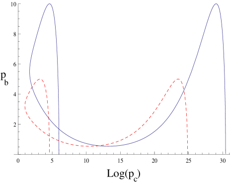
Figure 1: Plot shows the evolution for different mass black holes with same $L_{o}$(equal to unity). Solid (black) curve shows the evolution for $m=10$ and dashed (red) curve displays for $m=5$. Mass parameters are in Planck units and we use the conventional values $\Delta=4\sqrt{3}\pi\gamma{\ell}_{\rm Pl}^{2}$ and $\gamma=0.2375$.

The variation of $p_{b}$ and $p_{c}$ obtained by solving the above effective equations is shown in figures 1 and 2. The evolution starts from $p_{b}=0$ at the horizon. Classically the evolution breaks down at the singularity where both $p_{b}\rightarrow 0$ and $p_{c}\rightarrow 0$. This does not happen in the effective dynamics. In the high curvature regime, both $p_{c}$ and $p_{b}$ bounce and the singularity is avoided leading to a new white hole spacetime. Fig. 1, shows the effects of changing the mass parameter on the evolution. Fig. 2, displays the curves if one changes the auxiliary length $L_{o}$. As can be seen, it only translates the curve vertically without changing the value of the mass of the white hole. At the low curvature scales, the evolution approximates the classical theory.

To understand the details of the singularity resolution, let us consider the expansion ($\theta$) and shear ($\sigma^{2}$) scalars. These are given as follows:

$$\theta = \frac{1}{p_{b}}\frac{{\rm d}p_{b}}{{\rm d}\tau}+\frac{1}{2p_{c}}\frac{{\rm d}p_{c}}{{\rm d}\tau}$$ (57)

$$= \frac{1}{\gamma p_{c}^{1/2}}\Bigg{[}\frac{\sin(\delta_{b}b)}{\delta_{b}}(\cos(\delta_{b}b)+\cos(\delta_{c}c))$$

$$~{}~{}~{}~{}~{}~{}~{}~{}~{}~{}~{}~{}~{}~{}+\frac{\sin(\delta_{c}c)}{\delta_{c}}\cos(\delta_{b}b)\frac{p_{c}}{p_{b}}\Bigg{]}$$

and

$$\sigma^{2} = \frac{1}{3}\left(\frac{1}{p_{c}}\frac{{\rm d}p_{c}}{{\rm d}\tau}-\frac{1}{p_{b}}\frac{{\rm d}p_{b}}{{\rm d}\tau}\right)^{2}$$ (58)

$$= \frac{1}{3\gamma^{2}p_{c}^{1/2}}\Bigg{[}\frac{\sin(\delta_{b}b)}{\delta_{b}}(2\cos(\delta_{c}c)-\cos(\delta_{b}b))$$

$$~{}~{}~{}~{}~{}~{}~{}~{}~{}~{}~{}-\cos(\delta_{b}b)\frac{\sin(\delta_{c}c)}{\delta_{c}}\frac{p_{c}}{p_{b}}\Bigg{]}^{2}~{}.$$

In the classical theory, the expansion and shear scalars diverge at the central singularity where $p_{b}$ and $p_{c}$ vanish simultaneously. Since $p_{c}$ is bounded below, the dynamical evolution in the effective spacetime description does not allow $\theta$ and $\sigma^{2}$ to diverge when the central singularity is approached in the loop quantized model. Thus, the expansion and shear scalars are dynamically bounded and the central singularity is resolved. The boundedness of expansion and shear scalars is an indication that geodesics are complete in this effective spacetime, past the would-be singularity, as was the case for the isotropic and anisotropic models in LQC ps09 ; ps11 . Finally, we note that at the horizon the expansion and shear scalars diverge both in the classical theory and the effective theory because of the coordinate singularity encountered there.

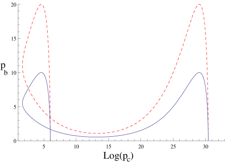
Figure 2: Effects of changing $L_{o}$ are displayed in the figure. For both curves we choose $m=10$ in Planck units. The solid (black) curve corresponds to $L_{o}=1$ and the dashed (red) curve to $L_{o}=2$. The mass of the white hole formed after bounce does not depend on $L_{o}$ and is equal for both cases independent of the choice of parameters.

It is important to note that the expansion and the shear scalars are free from the underlying freedom of the rescaling of the fiducial length $L_{o}$. This is in contrast to the Ashtekar-Bojowald prescription, where these scalars turn out to be dependent on the fiducial length ksbound . As has been stressed earlier by the authors, a consistency check of any quantization prescription is that the geometric scalars such as $\theta$ and $\sigma^{2}$ must be independent of any fiducial structure cs2 ; cs3 . Otherwise no consistent physical predictions on the details of the singularity resolution can be drawn from the quantization. So far, in the context of the black hole spacetimes the Böhmer-Vandersloot prescription was the only available quantization which satisfies this criteria ksbound . Our quantization prescription is the only other choice which passes this criteria, and which leads to a mathematically and physically consistent dynamics.

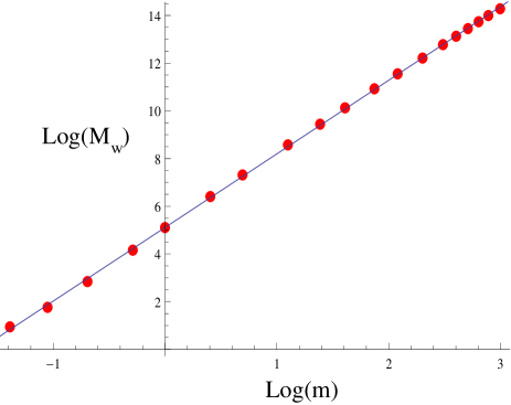
Figure 3: The (log of the) mass of the white hole $(M_{w})$ is plotted versus the (log of the) initial black hole mass $m$. It turns out that the white hole mass is proportional to an approximately cubic power of the starting black hole mass. The fit to the data points obtained from effective dynamics is $\log(M_{w})=5.1086+3.08679\log(m)$.

An interesting aspect of the effective dynamics in this quantization prescription is that the mass $M_{w}$ of the white hole which forms after the singularity resolution is directly determined by the original black hole mass $m$. The relation, for different initial conditions, between the black hole mass and the resulting white hole mass is shown in Fig. 3. Phenomenologically, we find that the white hole mass is approximately proportional to the cube of the black hole mass. Furthermore, we can explicitly see from the graph that the mass of the white hole is independent of the fiducial cell represented by $L_{o}$, thus satisfying our criteria for consistency.

Let us compare the results with earlier works in more detail. For the quantization of the Schwarzschild interior in Ref. aa:mb , an effective Hamiltonian was introduced in Ref. b-k which can be written using (46) after replacing $\delta_{b}$ and $\delta_{c}$ by a constant $\delta$. Note that departures from classical theory in the effective dynamics occur when trigonometric terms of the type $\sin(\delta c)$ in the effective Hamiltonian depart from $c$. The departures become most significant when the $\sin(\delta c)$ term saturates ($\sin(\delta c)\approx 1$). In the quantization proposed in Ref. aa:mb , the saturation of $\sin(\delta c)$ is not independent of the choice of auxiliary structure ($L_{o}$) introduced to define the phase space, since for $L_{o}\rightarrow\alpha L_{o}$: $c\rightarrow\alpha c$ and $\delta$ does not scale. (The term $\sin(\delta b)$ in the effective Hamiltonian though is independent of the rescaling in $L_{o}$). This is problematic as the dynamics then depends on the value of $L_{o}$ leading to unphysical effects. Hence, though we expect that fiducial structures should not affect physical predictions, the Ashtekar-Bojowald quantization prescription is an example where a theory fails this vital test.

Let us consider two instances in which the Ashtekar-Bojowald quantization yields inconsistent predictions. The first one is the minimum value of $p_{c}$ which depends on $L_{o}$ b-k . Since curvature scalars are proportional to inverse power of $p_{c}$, this implies that no sensible answer can be obtained for the upper bound on the value of spacetime curvature at which the bounce happens. The second example is the relation between the black hole mass $m$ and the white hole mass $M_{w}$. It was noted earlier that in the Ashtekar-Bojowald prescription the white hole mass is governed by the fiducial length $L_{o}$ (through $p_{b}^{(o)}$) b-k . Fig. 4 explicitly demonstrates this difference between the two quantization prescriptions. We plot solutions obtained from the effective dynamics in the Ashtekar-Bojowald prescription for two different choices of $L_{o}$ for the same black hole mass. Since in this approach there is no distinction between $\delta_{b}$ and $\delta_{c}$ and they are assumed to be constant, we have chosen $\delta=1$ in Fig. 4. We find that, in a striking comparison to the quantization put forward in this manuscript, the mass of the white hole changes with a change in $L_{o}$. Since the choice of the fiducial length $L_{o}$ is arbitrary, in the Ashtekar-Bojowald prescription the white hole can have an arbitrarily large or small mass which can be changed by a rescaling of $L_{o}$.

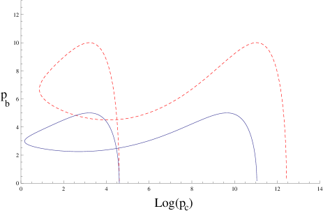
Figure 4: This figure corresponds to the case for quantization of Schwarzschild interior in Ref. aa:mb . Unlike the quantization presented in this manuscript (see Fig. 2), the mass of the white hole depends on the rescaling of $L_{o}$. For these simulations we have chosen $m=5$ in Planck units. The solid (black) curve corresponds to $L_{o}=1$ and the dashed (red) curve to $L_{o}=2$. By changing the fiducial scale $L_{o}$, the mass of the white hole can be changed arbitrarily in the quantization presented in Ref. aa:mb .

In contrast, in our approach the term $\sin(\delta_{c}c)$ in (46) does not depend on $L_{o}$. The reason is tied to the quantization presented here, leading to Eqs.(41). These imply that under the change $L_{o}\rightarrow\alpha L_{o}$: $\delta_{c}\rightarrow\alpha^{-1}\delta_{c}$, thus $\delta_{c}c\rightarrow\delta_{c}c$. Further, as in the previous case no effect is produced on the term $\sin(\delta_{b}b)$ under the rescaling of $L_{o}$. The saturation of $\sin(\delta_{c}c)$ and the resulting quantum gravitational effects are hence independent of the choice of $L_{o}$, which is seen from the plots in Fig. 2. As a consequence of all this, the mass $M_{w}$ of the white hole in our analysis turns out to be independent of any fiducial structure.

In summary, the reason for the success of our present quantization, when compared to the Ashtekar-Bojowald quantization, is the subtle difference in the way field strength is regulated in the quantum theory. The fact that subtleties in the quantization prescription can have a deep impact on the physical predictions of the theory is not new. Indeed, we have seen something rather similar in loop quantum cosmology. The old ($\mu_{o}$) quantization in LQC shared similar problems as the one in Ref. aa:mb , i.e. unacceptable dependence of physics on auxiliary structures. It was cured by the introduction of the ‘improved’ ($\bar{\mu}$) dynamics of LQC which resulted in change of the uniform discreteness variable from triad to volume aps2 . In the Schwarzschild case, no such change is needed. The quantum difference equation (44) is uniformly discrete in $p_{c}$ and $p_{b}$ as in the case of the earlier quantization aa:mb . Thus no refinement of the original lattice mb_cartin_khanna or ‘improvement’ on the lines of LQC b-k are required. All such ‘improved’ schemes suffer from the problem of predicting “quantum gravity” effects at low curvatures near the coordinate singularity at the horizon. Such unphysical effects near the horizon are absent in the present quantization.

VI Discussion

Let us summarize our results. In the process of quantizing the Schwarzschild interior, we have noted that an important step in the Hamiltonian formulation was the understanding of the physical length scale $r_{o}$ from the very beginning. This scale corresponds, in the classical description, precisely to the natural length scale in the system, the Schwarzschild radius. This simple modification has important ramifications. For, in the heart of the loop quantization, namely in the replacement of curvature by finite holonomies, there are two unequal parameters $\delta_{b}$ and $\delta_{c}$. The former depending on $r_{o}$ and the latter on the auxiliary length scale $L_{o}$. As a consequence, the resulting Hamiltonian operator is invariant under the change of fiducial cell. In this respect, the quantization found here can be seen as a refinement of that in Ref. aa:mb . In particular, it reduces to that one when the parameter in each direction are set to be equal. An important feature of the resulting quantum constraint is that it is perfectly regular at the ‘would be singularity’. Physics does not stop there.

Even when we do not have a physical Hilbert space and Dirac operators thereon, one can expect that effective equations describe the unitary evolution of appropriate semiclassical states, as happens in multiple examples within the isotropic sector. We have analysed in detail these effective equations and found interesting dynamics. In the relevant variable chosen the ‘initial condition’ is given by the model universe (of spatial topology $\mathbb{S}^{2}\times\mathbb{R}$) approaching a null surface, that in the Schwarzschild solution corresponds to the (black hole) event horizon. The homogeneous hypersurfaces contract as they would in Schwarzschild but, instead of reaching zero area in a finite proper time (the singularity), the spheres reach a minimum value of area and ‘bounce back’, approaching a different constant value in the asymptotic future. This asymptotic value (that could be called the mass of a white hole) only depends on the mass of the original black hole and does not depend on the other degree of freedom available in the Hamiltonian description, nor on any fiducial structure. Analysis of the solutions of the effective equations show that the mass of the white hole is proportional to the cube of the starting black hole mass. In both asymptotic past and future, where the classical horizons might arise, the dynamics from the effective Hamiltonian approximates the classical dynamics. Thus, there are no spurious quantum gravity effects appearing where one does not expect them. Our quantization represents the first one possessing all these features. Further, analysis of the expansion and shear scalars shows that they are dynamically bounded on the approach to the classical singularity and are free from the rescaling of fiducial structures. These results stand in striking contrast to the resulting physics derived from the effective description of the Ashtekar-Bojowald quantization where the white hole mass, and the expansion and shear scalars depended on the fiducial length $L_{o}$. Finally, we would like to end this note with two remarks.

Relation with the Information loss issue. The singularity resolution found in Ref. aa:mb gave support to the paradigm proposed in aa-mb-info about black hole evaporation and information loss (further support comes from work in the CGHS model cghs ). The basic idea is that the scenario in which a black hole looses mass via Hawking radiation and evaporates is based in the assumption that there exists a singularity inside the event horizon. If, as (loop) quantum gravity effects suggest, there is no singularity, then one has to conclude that there was no event horizon to begin with and one has to extend the arena on which to describe the physical process, from the standard one with a future singularity to some ‘quantum spacetime’ containing no singularity. What can we say from our present study regarding this issue? The problem we have analysed is posed with the initial conditions corresponding to a space-like surface ‘just inside’ the event horizon of the Schwarzschild spacetime, and through dynamical evolution, after the bounce the asymptotic geometry to the future approaches that of a space-like surface ‘just inside’ a white-hole horizon of a different mass. While in the restricted sense of our analysis (vacuum and therefore no backreaction of matter), one obtains a different asymptotic region to the future, one can not conclude that the new paradigm does not hold. In order to settle this question, one would need a more complete treatment, including radiating matter, and an extension to the exterior region of the horizon. It is only with that more complete description that one might hope to give meaning to the ‘effective spacetime’ that arises from the solution to our effective equations, in terms of the Ashtekar-Bojowald paradigm aa-mb-info . In particular it should be clear that from the perspective of a complete non-singular quantum state, statements like ‘the mass of the initial black hole’ or ‘final white hole’ might become meaningless. Needless to say, a lot of work in this direction is needed, and our present analysis can only be seen as a first step in that direction.

Relation to $2+1$ Gravity. In several instances, it has been useful to relate 3+1 symmetric spacetimes, via the Geroch reduction, to $2+1$ gravity coupled to a massless scalar field $\psi$ geroch . This equivalence has been exploited to study the quantum theory of Einstein Rosen waves ER and polarized Gowdy models pierri . For the Kantowski-Sachs model under consideration here, this strategy is also a possibility that one might consider. To be precise, we have for the Schwarzschild interior all the ingredients needed in such reduction, namely, a Killing field $\xi=\partial/\partial x$ that is hypersurface orthogonal (to the $x=$constant surfaces). Thus, any Kantowski-Sachs space-time (in vacuum) is equivalent to a spherically symmetric gravitational field $\tilde{g}_{ab}$ on a 3D spacetime with topology ${}^{3}\!{\cal M}=\mathbb{S}^{2}\times\mathbb{R}$, coupled to a mass-less spherically symmetric scalar field $\psi$. The scalar field is proportional to the logarithm of the norm of $\xi$ (given by $g_{xx}$). If we analyse the system from this perspective we see that the 3D Ricci curvature $\tilde{R}_{ab}$ (and energy density of the scalar field as defined by the 3D energy momentum tensor $\tilde{T}_{ab}$) diverge at both the $t=0$ singularity and at the horizon where $t=2m$. The spurious curvature singularity at the horizon of the 3D metric $\tilde{g}$ disappears once we go back to the $3+1$ description by means of the conformal transformation that relates both metrics and that in this case ‘cures’ the singularity, yielding a finite 4D curvature at the horizon. It is to be noted that any quantization that was build from the $2+1$ perspective and that was successful in ‘curing’ this 3D singularity would be, however, physically inadequate from the 4D perspective, where no classical singularity exists. In fact, what one might conclude is that the ‘improved’ schemes of b-k and cs2 ; cs3 are somewhat tailored to curing this 3D singularity as well, as can be seen from the fact that spurious quantum gravity effects appear near the horizon. In retrospect, this is not the first instance in which the classical equivalence between 4D symmetric models and $2+1$ gravity $+$ scalar field faces some difficulties in the quantum realm. In the case of polarized Gowdy models, the resulting quantization that used this equivalence in a fundamental way does not possess a unitary time evolution CCQ . Furthermore, it has been shown that no such quantization exists for that field parametrization CMV . In order to have a consistent, unitary, description one needs to take the 4D character of the problem at face value and find a suitable parametrization that does not admit a $2+1$ interpretation CCM .

References

- (1) A. Ashtekar and J. Lewandowski “Background independent quantum gravity: A status report,” Class. Quant. Grav. 21 (2004) R53 arXiv:gr-qc/0404018; C. Rovelli, “Quantum Gravity”, (Cambridge U. Press, 2004); T. Thiemann, “Modern canonical quantum general relativity,” (Cambridge U. Press, 2007).
- (2) A. Ashtekar and P. Singh, “Loop Quantum Cosmology: A Status Report,” Class. Quant. Grav. 28, 213001 (2011) arXiv:1108.0893 [gr-qc]; I. Agullo and A. Corichi, “Loop Quantum Cosmology,” The Springer Handbook of Spacetime, Springer-Verlag (2014) arXiv:1302.3833 [gr-qc]
- (3) A. Ashtekar, T. Pawlowski and P. Singh, “Quantum nature of the big bang: Improved dynamics,” Phys. Rev. D 74, 084003 (2006) arXiv:gr-qc/0607039.
- (4) A. Ashtekar, A. Corichi and P. Singh, “Robustness of key features of loop quantum cosmology,” Phys. Rev. D 77, 024046 (2008). arXiv:0710.3565 [gr-qc].
- (5) P. Singh, “Numerical loop quantum cosmology: an overview,” Class. Quant. Grav. 29, 244002 (2012) arXiv:1208.5456 [gr-qc]]; D. Brizuela, D. Cartin and G. Khanna, “Numerical techniques in loop quantum cosmology,” SIGMA 8, 001 (2012) [arXiv:1110.0646 [gr-qc]]
- (6) A. Ashtekar, M. Bojowald, “Quantum geometry and the Schwarzschild singularity,” Class. Quant. Grav. 23, 391 (2006). arXiv:gr-qc/0509075.
- (7) L. Modesto, “Loop quantum black hole,” Class. Quant. Grav. 23, 5587 (2006) arXiv:gr-qc/0509078.
- (8) M. Campiglia, R. Gambini and J. Pullin, “Loop quantization of spherically symmetric midi-superspaces : the interior problem,” AIP Conf. Proc. 977, 52 (2008) arXiv:0712.0817 [gr-qc].
- (9) R. Gambini and J. Pullin, “Loop quantization of the Schwarzschild black hole,” Phys. Rev. Lett. 110, 211301 (2013) arXiv:1302.5265 [gr-qc]]
- (10) C. G. Boehmer and K. Vandersloot, “Loop Quantum Dynamics of the Schwarzschild Interior,” Phys. Rev. D 76, 104030 (2007); arXiv:0709.2129[gr-qc].
- (11) A. Ashtekar, M. Bojowald and L. Lewandowski, “Mathematical structure of loop quantum cosmology” Adv. Theor. Math. Phys. 7 233 (2003) arXiv:gr-qc/0304074.
- (12) A. Ashtekar, T. Pawlowski and P. Singh, “Quantum Nature of the Big Bang: An Analytical and Numerical Investigation. I.,” Phys. Rev. D 73, 124038 (2006) gr-qc/0604013
- (13) A. Corichi and P. Singh, “Is loop quantization in cosmology unique?,” Phys. Rev. D 78, 024034 (2008) arXiv:0805.0136 [gr-qc]
- (14) A. Corichi and P. Singh, “A Geometric perspective on singularity resolution and uniqueness in loop quantum cosmology,” Phys. Rev. D 80, 044024 (2009) arXiv:0905.4949 [gr-qc]
- (15) A. Joe and P. Singh, “Kantowski-Sachs spacetime in loop quantum cosmology: bounds on expansion and shear scalars and the viability of quantization prescriptions,” Class. Quant. Grav. 32, no. 1, 015009 (2015) arXiv:1407.2428 [gr-qc]
- (16) M. Bojowald, D. Cartin and G. Khanna, “Lattice refining loop quantum cosmology, anisotropic models and stability,” Phys. Rev. D 76, 064018 (2007) arXiv:0704.1137 [gr-qc].
- (17) N. Dadhich, A. Joe and P. Singh, “Emergence of product of constant curvature spaces in loop quantum cosmology,” arXiv:1505.05727 [gr-qc]
- (18) A. Joe, P. Singh, Phenomenological aspects of Kantowski-Sachs spacetimes in LQC (To appear).
- (19) A. Ashtekar and B. Krishnan, “Isolated and dynamical horizons and their applications,” Living Rev. Rel. 7, 10 (2004) [arXiv:gr-qc/0407042].
- (20) P. Diener, B. Gupt, P. Singh, “Numerical simulations of a loop quantum cosmos: robustness of the quantum bounce and the validity of effective dynamics,” Class. Quant. Grav. 31, 105015 (2014) arXiv:1402.6613 [gr-qc]]; P. Diener, B. Gupt, M. Megevand, P. Singh, “Numerical evolution of squeezed and non-Gaussian states in loop quantum cosmology,” Class. Quant. Grav. 31, 165006 (2014) arXiv:1406.1486 [gr-qc]]
- (21) D. W. Chiou, “Phenomenological loop quantum geometry of the Schwarzschild black hole,” Phys. Rev. D 78, 064040 (2008) [arXiv:0807.0665 [gr-qc]]
- (22) P. Singh, “Are loop quantum cosmos never singular?,” Class. Quant. Grav. 26, 125005 (2009) arXiv:0901.2750 [gr-qc]
- (23) P. Singh, “Curvature invariants, geodesics and the strength of singularities in Bianchi-I loop quantum cosmology,” Phys. Rev. D 85, 104011 (2012) arXiv:1112.6391 [gr-qc]
- (24) A. Ashtekar and M. Bojowald, “Black hole evaporation: A paradigm,” Class. Quant. Grav. 22, 3349 (2005); arXiv:gr-qc/0504029.
- (25) A. Ashtekar, V. Taveras, M. Varadarajan, ‘ ‘Information is Not Lost in the Evaporation of 2-dimensional Black Holes,” Phys. Rev. Lett. 100, 211302 (2008); arXiv:0801.1811[gr-qc]; A. Ashtekar, F. Pretorius and F. M. Ramazanoglu, “Evaporation of 2-Dimensional Black Holes,” Phys. Rev. D 83, 044040 (2011) doi:10.1103/PhysRevD.83.044040 arXiv:1012.0077 [gr-qc].
- (26) R. Geroch, “A Method for generating solutions of Einstein’s equations,” J. Math. Phys. 12, 918 (1971).
- (27) A. Ashtekar and M. Pierri, “Probing quantum gravity through exactly soluble midi-superspaces. I,” J. Math. Phys. 37, 6250 (1996) arXiv:gr-qc/9606085.
- (28) M. Pierri, “Probing quantum general relativity through exactly soluble midi-superspaces. II: Polarized Gowdy models,” Int. J. Mod. Phys. D 11, 135 (2002) arXiv:gr-qc/0101013.
- (29) A. Corichi, J. Cortez and H. Quevedo, “On unitary time evolution in Gowdy T(3) cosmologies,” Int. J. Mod. Phys. D 11, 1451 (2002) arXiv:gr-qc/0204053; C. G. Torre, “Quantum dynamics of the polarized Gowdy model,” Phys. Rev. D 66, 084017 (2002) arXiv:gr-qc/0206083.
- (30) J. Cortez, G. A. Mena Marugan and J. M. Velhinho, “Uniqueness of the Fock quantization of the Gowdy model,” Phys. Rev. D 75, 084027 (2007) arXiv:gr-qc/0702117.
- (31) A. Corichi, J. Cortez and G. A. Mena Marugan, “Quantum Gowdy model: A unitary description,” Phys. Rev. D 73, 084020 (2006) arXiv:gr-qc/0603006.