A. Garbuno-Inigo, F.A. DiazDelaO, K.M. Zuev, Gaussian process hyper-parameter estimation using Parallel Asymptotically Independent Markov Sampling, Computational Statistics & Data Analysis, Volume 103, November 2016.
Gaussian process hyper-parameter estimation using parallel asymptotically independent Markov sampling

Abstract

Gaussian process emulators of computationally expensive computer codes provide fast statistical approximations to model physical processes. The training of these surrogates depends on the set of design points chosen to run the simulator. Due to computational cost, such training set is bound to be limited and quantifying the resulting uncertainty in the hyper-parameters of the emulator by uni-modal distributions is likely to induce bias. In order to quantify this uncertainty, this paper proposes a computationally efficient sampler based on an extension of Asymptotically Independent Markov Sampling, a recently developed algorithm for Bayesian inference. Structural uncertainty of the emulator is obtained as a by-product of the Bayesian treatment of the hyper- parameters. Additionally, the user can choose to perform stochastic optimisation to sample from a neighbourhood of the Maximum a Posteriori estimate, even in the presence of multimodality. Model uncertainty is also acknowledged through numerical stabilisation measures by including a nugget term in the formulation of the probability model. The efficiency of the proposed sampler is illustrated in examples where multi-modal distributions are encountered. For the purpose of reproducibility, further development, and use in other applications the code used to generate the examples is freely available for download at https://github.com/agarbuno/paims_codes.

1 Introduction

Computationally expensive computer codes are frequently needed to implement mathematical models which are assumed to be reliable approximations to physical processes. Such simulators often require intensive use of computational resources that makes them inefficient if further exploitation of the code is needed, e.g. optimisation, uncertainty propagation and sensitivity analysis (Forrester et al., 2008, Kennedy and O’Hagan, 2001a). For this reason, surrogate models are needed to perform fast approximations to the output of demanding simulators and enable efficient exploration and exploitation of the input space. In this context, Gaussian processes are a common choice to build statistical surrogates -also known as emulators- which allow to take into account the uncertainty derived from the inability to evaluate the original model in the whole input space. Gaussian processes have become popular in recent years due to their ability to fit complex mappings between outputs and inputs by means of a non-parametric hierarchical structure. Such applications are found, amongst many other areas, in Machine Learning (Rasmussen and Williams, 2006), Spatial Statistics (Cressie, 1993) (with the name of Kriging), likelihood-free Bayesian Inference (Wilkinson, 2014) and Genetics (Kalaitzis and Lawrence, 2011).

To build an emulator, a number of runs from the simulator is needed, but due to computing limitations only a small amount of evaluations can be performed. With a small amount of data, it is possible that the uncertainty of the parameters of the model cannot be described by a clearly uni-modal distribution. In such scenarios, Model Uncertainty Analysis (Draper, 1995) is capable of setting a proper framework in which we acknowledge all uncertainties related to the idealisations made through the modelling assumptions and the available, albeit limited information. To this end, hierarchical modelling should be taken into account. This corresponds to adding a layer of structural uncertainty to the assumed emulator either in a continuous or discrete manner (see Draper, 1995, §4). In the case of Gaussian processes, continuous structural uncertainty can be accounted for as a natural by-product from a Bayesian procedure. Hence, this is pursued in this work by focusing on samplers capable of exploring multi-modal distributions.

In order for the Gaussian process to be able to replicate the relation between inputs and outputs and make predictions, a training phase is necessary. Such training involves the estimation of the parameters of the Gaussian process from the data collected by running the simulator. These parameters are referred to as hyper-parameters. The selection of the hyper-parameters is usually done by using Maximum Likelihood estimates (MLE), or their Bayesian counterpart Maximum a Posteriori estimates (MAP) (Oakley, 1999, Rasmussen and Williams, 2006), or by sampling from the posterior distribution (Williams and Rasmussen, 1996) in a fully Bayesian manner.

In this paper we assume a scenario where the task of generating new runs from the simulator is prohibitive. Such limited information is not enough to completely identify either a candidate or a region of appropriate candidates for the hyper-parameters. In this scenario, traditional optimisation routines (Nocedal and Wright, 2004) are not able to guarantee global optima when looking for the MLE or MAP, and a Bayesian treatment is the only option to account for all the uncertainties in the modelling. In the literature, however, it is common to see that MLE or MAP alternatives are preferred (Kennedy and O’Hagan, 2001a, Gibbs, 1998) due to the numerical burden of maximising the likelihood function or because it is assumed that Bayesian integration will not produce results worth the effort. Though it is a strong argument in favour of estimating isolated candidates, in high-dimensional applications it is difficult to assess if the number of runs of the simulator is sufficient to produce robust hyper-parameters. Robustness is usually measured with a prediction-oriented metric such as root-mean-square error (RMSE) (Kennedy and O’Hagan, 2001b), ignoring uncertainty and risk assessment of choosing a single candidate of the hyper-parameters by an inference process with limited data. In order to account for such uncertainty in the hyper-parameters when making predictions, numerical integration should be performed. However, methods as quadrature approximation become infeasible as the number of dimensions increases (Kennedy and O’Hagan, 2001a). Therefore, an appropriate approach is to perform Monte Carlo integration (MacKay, 1998). This allows to approximate any integral by means of a weighted sum, given a sample from the correct distribution.

In Gaussian processes, as in many other applications of statistics, the target distribution of the hyper-parameters cannot be sampled directly and one should resort to Markov Chain Monte Carlo (MCMC) methods (Robert and Casella, 2004). MCMC methods are powerful statistical tools but have a number of drawbacks if not tuned properly, particularly if one wishes to sample from multi-modal distributions (Neal, 2001, Hankin, 2005). One of such limitations is the tuning of the proposal distribution, which allows the generation of a candidate in the chain. This proposal function has to be tuned with parameters that define its ability to move through the sample space. If an excessively wide spread is selected, this will produce samples with space-filling properties but which are likely to be rejected. On the other hand, having a narrower spread will cause an inefficient exploration of the sample space by taking short updates of the states of the chain, known in the literature as Random Walk behaviour (Neal, 1993). In practice it is desirable to use a proposal distribution which is capable of balancing both extremes. To find an appropriate tuning in high-dimensional spaces with sets of highly correlated variables can be an overwhelming task and often MCMC samplers can become expensive due to the long time needed to reach stationarity (Ching and Chen, 2007). Neal (1998) and Williams and Rasmussen (1996) favour the Hybrid Monte Carlo (HMC) method to generate a sample from the posterior distribution, preventing the random walk behaviour of traditional MCMC methods. If tuned correctly, the HMC should be able to explore most of the input space (Liu, 2008). Such tuning process is problem-dependent and there is no guarantee that the method will sample from all existing modes, thus failing to adapt well to multi-modal distributions (Neal, 2011).

This paper proposes a sampler for the hyper-parameters of a Gaussian process based on recently developed methods for Bayesian inference problems. Additionally, it uses the Transitional Markov Chain Monte Carlo (TMCMC) method of Ching and Chen (2007) to set a framework for the parallelisation of Asymptotically Independent Markov Sampling in both the context of hyper-parameter sampling (AIMS) (Beck and Zuev, 2013) and in stochastic optimisation (AIMS-OPT) (Zuev and Beck, 2013) reminiscent of Stochastic Subset Optimisation (Taflanidis and Beck, 2008a, b). Such an extension is built using concepts of Particle Filtering methods (Andrieu et al., 2010, Gramacy and Polson, 2009), Adaptive Sequential Monte Carlo (Del Moral et al., 2006, 2012) and Delayed Rejection Samplers (Zuev and Katafygiotis, 2011, Mira, 2001). AIMS is chosen since it provides a framework for Sequential Monte Carlo sampling (Neal, 1996, 2001, Del Moral et al., 2006) which automatically chooses the sequence of transitions. Moreover, it uses most of the information generated in the previous step in the sequence as opposed to traditional sequential methods, thus building a robust sampler when applied to multi-modal distributions. Finally, by using the AIMS-OPT algorithm a solution is built by means of a nested sequence of subsets, which converges to the optimal solution set. The algorithm can be terminated prematurely given a previously chosen accuracy threshold, thus providing a set of nearly optimal solutions. Whether it is composed by a single element, or a set of elements whose objective function differs by a negligible quantity, a full characterisation of the optimal solution is achieved. This contrasts with the capabilities of other stochastic optimisation schemes such as particle swarm optimisation or genetic algorithms (Schneider and Kirkpatrick, 2007).

By selecting the hyper-parameters using the AIMS-OPT framework the effect is twofold. First, the uncertainty inherent to the specification of the hyper-parameters is embedded in the set of suboptimal approximations to the solution. This uncertainty, expressed in a mixture of Gaussian process emulators, yields a robust surrogate where model uncertainty is accounted for. Second, computational implementation deficiencies of the inference procedure in Gaussian processes is overcome by incorporating stabilising approaches exposed in the literature as in Ranjan et al. (2011), Andrianakis and Challenor (2012) but in a Bayesian framework. The problem is therefore treated from both a probabilistic and an optimisation perspective.

The paper is organised as follows. In Section 2, a brief introduction to the Gaussian processes and their treatment by Bayesian inference is discussed. Section 3 presents both the AIMS algorithm and the proper generalisation for a parallel implementation. Section 4 discusses several aspects of the computational implementation of the algorithm and their effect on the modelling assumptions. The efficiency and robustness of the proposed sampler are discussed in Section 5 with some illustrative examples. Concluding remarks are given in Section 6.

2 Gaussian processes

Let $X=\{\mathbf{x}_{1},\ldots,\mathbf{x}_{n}\}$ be the set of trials run by the simulator where $\mathbf{x}_{i}\in\mathbb{R}^{p}$ denotes a given configuration for the model. The set $X$ will be referred to as the set of design points. Let $\mathbf{y}=\{y_{1},\ldots,y_{n}\}$ be the set of outputs observed for the design points. The pair $(\mathbf{x}_{i},y_{i})$ will denote the training run being used to learn the emulator that approximates the simulator. The emulator is assumed to be a real-valued mapping $\eta:\mathbb{R}^{p}\rightarrow\mathbb{R}$ which is an interpolator of the training runs, i.e. $y_{i}=\eta(\mathbf{x}_{i})$ for all $i=1,\ldots,n$. This omits any random error in the output of the computer code in the observed simulations, that is, the simulator is deterministic. It is assumed that the output of the simulator can be represented by a Gaussian process. Therefore, the set of design points is assumed to have a joint Gaussian distribution where the output satisfies the structure

$$\eta(\mathbf{x})=h(\mathbf{x})^{T}\boldsymbol{\beta}+Z(\mathbf{x}|\sigma^{2},\boldsymbol{\phi}),$$ (2.1)

where $h(\cdot)$ is a vector of known basis (location) functions of the input, $\boldsymbol{\beta}$ is a vector of regression coefficients, and $Z(\cdot|\sigma^{2},\boldsymbol{\phi})$ is a Gaussian process with zero mean and covariance function

$$\text{cov}(\mathbf{x},\mathbf{x}^{\prime}|\sigma^{2},\boldsymbol{\phi})=\sigma^{2}\,k(\mathbf{x},\mathbf{x}^{\prime}|\boldsymbol{\phi}),$$ (2.2)

where $\sigma^{2}$ is the signal noise and $\boldsymbol{\phi}\in\mathbb{R}^{p}_{+}$ denotes the length-scale parameters of the correlation function $k(\cdot,\cdot)$. Note that for a pair of design points$(\mathbf{x},\mathbf{x}^{\prime})$, the function $k(\cdot,\cdot|\boldsymbol{\phi})$ measures the correlation between $\eta(\mathbf{x})$ and $\eta(\mathbf{x}^{\prime})$ based on their respective input configurations. The effect of different values of $\boldsymbol{\phi}$ in a one-dimensional example is depicted in Figure 1.

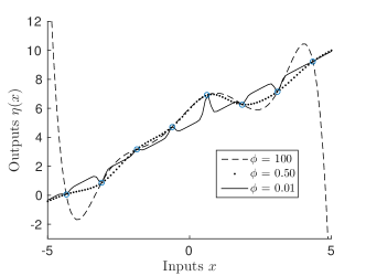
Figure 1: The length-scale parameters represent how sensitive is the output of the simulator to variations in each dimension. The plot corresponds to 8 design points chosen for the function $\eta(x)=5+x+\cos(x)+.5\,\sin(3x)$. For low values of the length-scale parameter the training runs are less dependent of each other.

The role of the correlation function is to measure how close to each other the design points are, following the assumption that similar input configurations should produce similar outputs. For its analytical simplicity, interpretation and smoothness properties, this work uses the squared-exponential correlation function, namely

$$k(\mathbf{x},\mathbf{x}^{\prime}|\boldsymbol{\phi})=\exp\left\{-\frac{1}{2}\displaystyle\sum_{i=1}^{p}\frac{(x_{i}-x^{\prime}_{i})^{2}}{\phi_{i}}\right\}.$$ (2.3)

Note that other authors prefer the parametrisation with $\phi^{2}_{i}$ as denominators. However, this work uses a linear term in the denominator since the restriction of the length-scale parameters to lie in the positive orthant is more natural, as weights in the norm used to measure closeness and sensitivity to changes in such dimensions. Both interpretability and numerical performance can be improved if the length-scales refer to the same units, which leads to rescaling all dimensions of the input configurations. In the computer simulation terminology this translates in utilising experimental designs restricted to hypercubes, such as Latin hypercube sampling or Sobol sequences. Design of experiments is an active area of research outside the scope of this work.

In summary, the output of a design point, given the parameters $\boldsymbol{\beta},\sigma^{2}$ and $\boldsymbol{\phi}$, has a Gaussian distribution

$$y|\mathbf{x},\boldsymbol{\beta},\sigma^{2},\boldsymbol{\phi}\sim\mathcal{N}(h(\mathbf{x})^{T}\boldsymbol{\beta},\sigma^{2}\,k(\mathbf{x},\mathbf{x}^{\prime}|\boldsymbol{\phi})),$$ (2.4)

which can be rewritten as the joint distribution of the vector of outputs $\mathbf{y}$ conditional on the design points $X$ and hyper-parameters $\boldsymbol{\beta},\sigma^{2}$ and $\boldsymbol{\phi}$ as

$${\bf y}|X,\boldsymbol{\beta},\sigma^{2},\boldsymbol{\phi}\sim\mathcal{N}(H\boldsymbol{\beta},\sigma^{2}\,K),$$ (2.5)

where $H$ is the design matrix whose rows are the inputs $h(\mathbf{x}_{i})^{T}$ and $K$ is the correlation matrix with elements $K_{ij}=k(\mathbf{x}_{i},\mathbf{x}_{j}|\boldsymbol{\phi})$ for all $i,j=1,\ldots,n$.

2.1 Estimating the hyper-parameters

The parameters of the process are not known beforehand and this induces uncertainty in the emulator itself. They can be estimated by Maximum Likelihood principles, but doing so lacks rigorous uncertainty quantification by concentrating all the density of the unknown quantities in a single value. The alternative is to treat them in a fully Bayesian manner and marginalise them when performing predictions. This way their respective uncertainty is taken into account. In this scenario, the prediction $y^{*}$ for a non-observed configuration $\mathbf{x}^{*}$ can be performed with the data available, $\mathcal{D}=({\bf y},X)$, and the evidence they shed on the parameters of the Gaussian process. Therefore, the predictions should be made with the marginalised posterior distribution

$$p(y^{*}|\mathbf{x}^{*},\mathcal{D})=\int_{\Theta}p(y^{*}|\mathbf{x}^{*},\mathcal{D},\boldsymbol{\theta})\,p(\boldsymbol{\theta}|\mathcal{D})\,d\boldsymbol{\theta},$$ (2.6)

where $\boldsymbol{\theta}=(\boldsymbol{\beta},\sigma^{2},\boldsymbol{\phi})$ denotes the complete vector of hyper-parameters. One should note that given the properties of a collection of Gaussian random variables, a prediction for $y^{*}$ conditioned in the data and $\boldsymbol{\theta}$ is also a Gaussian random variable (see Oakley, 1999). As in hierarchical modelling, each possible value of $\boldsymbol{\theta}$ defines a specific realisation of a Gaussian distribution, so it is appropriate to refer to $\boldsymbol{\theta}$ as the hyper-parameters of the Gaussian process.

Due to its computational complexity, the integral in (2.6) is often omitted when making predictions. It is commonly assumed that the MLE of the likelihood

$$\mathcal{L}(\boldsymbol{\theta})=p(\mathbf{y}|X,\boldsymbol{\beta},\sigma^{2},\boldsymbol{\phi}),$$ (2.7)

or the MAP estimate from the posterior distribution

$$p(\boldsymbol{\theta}|\mathcal{D})\propto p({\bf y}|X,\boldsymbol{\beta},\sigma^{2},\boldsymbol{\phi})\,\,p(\boldsymbol{\beta},\sigma^{2},\boldsymbol{\phi}),$$ (2.8)

are robust enough to account for all the uncertainty in the modelling. However, when either the likelihood (2.7) is a non-convex function or the posterior (2.8) is a multi-modal distribution, conventional optimisation routines might only find local optima, thus failing to find the most probable candidate of such distribution. Moreover, by selecting only one candidate, robustness and uncertainty quantification are lost in the process. Additionally, there are degenerate cases when it is crucial to estimate the integral in (2.6) by means of Monte Carlo simulation instead of by proposing a single candidate. As it has been noted by Andrianakis and Challenor (2012), two extreme cases for the Gaussian process length-scale hyper-parameters can be identified. One possibility is for $\phi$ to approach infinity, which makes every design point dependent of each other; the other, when $\phi$ approaches the origin where a multivariate regression model becomes the limiting case. In the first case, high correlation among all the training runs results in a model which is not able to distinguish local dependencies. As for the second, it violates the assumptions that constitute a Gaussian process, by completely ignoring the correlation structure in the design points to predict the output. Consequently, if MCMC is performed one can approximate the integrated predictive distribution in (2.6) by means of

$$p(y^{*}|\mathbf{x}^{*},\mathcal{D})\approx\sum_{i=1}^{N}w_{i}\,\,p(y^{*}|\mathbf{x}^{*},\mathcal{D},\boldsymbol{\theta}_{i}),$$ (2.9)

where $\boldsymbol{\theta}_{i}$ is obtained through an appropriate sampler, i.e. one capable of sampling from multi-modal distributions. The coefficients $w_{i}$ denote the weights of each sample generated. Since each term $p(y^{*}|\mathbf{x}^{*},\mathcal{D},\boldsymbol{\theta}_{i})$ corresponds to a Gaussian density function, the predictions are made by a mixture of Gaussians.

Proposition 1.

If the emulator output $y^{*}$ conditional on its configuration vector $\mathbf{x}^{*}$ has a posterior density as in (2.9), then its mean function and covariance function can be computed as

$$\mu(\mathbf{x}^{*}) =\sum_{i=1}^{N}w_{i}\,\,\mu_{i}(\mathbf{x}^{*}),$$ (2.10)

$$\text{cov}(\mathbf{x}^{*},\mathbf{x}^{\prime}) =\sum_{i=1}^{N}w_{i}\,\,\left[(\mu_{i}(\mathbf{x}^{*})-\mu(\mathbf{x}^{*}))(\mu_{i}(\mathbf{x}^{\prime})-\mu(\mathbf{x}^{\prime}))+\text{cov}(\mathbf{x}^{*},\mathbf{x}^{\prime}|\boldsymbol{\theta}_{i})\right],$$ (2.11)

where $\mu_{i}(\mathbf{x}^{*})$ denotes the expected value of the likelihood distribution of $y^{*}$ conditional on the hyper-parameters $\boldsymbol{\theta}_{i}$, the training runs $\mathcal{D}$ and the input configuration $\mathbf{x}^{*}$.

Proof.

Equality in (2.10) is a direct application of the tower property of conditional expectation and (2.11) follows from the covariance decomposition formula using the vector of weights $w_{i}$ as an auxiliary probability distribution on the conditioning. ∎

From equation (2.11) we can compute the variance, also known as the prediction error, of an untested configuration $\mathbf{x}^{*}$ as

$$\text{var}(\mathbf{x^{*}}) =\sum_{i=1}^{N}w_{i}\,\,((\mu_{i}(\mathbf{x^{*}})-\mu(\mathbf{x^{*}}))^{2}+\sigma_{i}^{2}(\mathbf{x^{*}})).$$ (2.12)

By doing this, a more robust estimation of the prediction error is made since it balances the predicted error in one sample with how far the prediction of such sample is from the overall estimation of the mixture.

2.2 Prior distributions

In order to perform a Bayesian treatment for the prediction task in equation (2.6) the prior distribution $p(\boldsymbol{\beta},\sigma^{2},\boldsymbol{\phi})$ in equation (2.8) has to be specified. Weak prior distributions are commonly used for $\boldsymbol{\beta}$ and $\sigma^{2}$ (Oakley, 1999). Such weak prior has the form

$$p(\boldsymbol{\beta},\sigma^{2},\boldsymbol{\phi})\propto\frac{p(\boldsymbol{\phi})}{\sigma^{2}},$$ (2.13)

where it is assumed a priori that both the covariance and the mean hyper-parameters are independent. Even more, $\boldsymbol{\beta}$ and $\sigma^{2}$ are assumed to have an improper non-informative distribution.

As for the length-scale hyper-parameter $\boldsymbol{\phi}$, a prior distribution $p(\boldsymbol{\phi})$ is still needed. In this case the reference prior (studied by Berger and Bernardo, 1992, Berger et al., 2009) sets an objective framework to account for the uncertainty of $\boldsymbol{\phi}$, thus avoiding any potential bias induced by the modelling assumptions. This prior is built based on Shannon’s expected information criteria and allows the use of a prior distribution in a setting where no previous knowledge is assumed. That way, the training runs are the only source of information for the inference process. Additionally, the reference prior is capable of ruling out subspaces of the sample space of the hyper-parameters (Andrianakis and Challenor, 2011), thus reducing regions of possible candidates of Gaussian distributions in the mixture model in equation (2.9). Since this provides an off-the-shelf framework for the estimation of the hyper-parameters, the reference prior developed by Paulo (2005) is used in this work. However, there are no known analytical expressions for its derivatives which limits its application to MCMC samplers that use gradient information. Note that there are other possibilities available for the prior distribution of $\boldsymbol{\phi}$. Examples of these are the log-normal or log-Laplacian distributions, which can be interpreted as a regularisation in the norm of the parameters. Andrianakis and Challenor (2011) suggest a decaying prior. Another option is to elicit prior distributions from expert knowledge as in Oakley (2002).

2.3 Marginalising the nuisance hyper-parameters

The nature of the hyper-parameters $\boldsymbol{\beta},\sigma^{2}$ and $\boldsymbol{\phi}$ is potentially different in terms of scales and dynamics, as seen and explained in Figure 2. It is possible to cope with this limitations by using a Gibbs sampling framework, but it is well-known that such sampling scheme can be inefficient if it is used for multi-modal distributions in higher dimensions. Analogously, a Metropolis-Hastings sampler can also be overwhelmed.

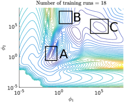
((a)) Correlations

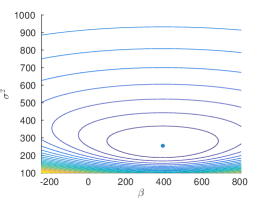
((b)) Scales

Figure 2: In 2(a), different dynamics of the hyper-parameters for the log-posterior distribution of test function 5.1 are shown: A. corresponds to positive correlation. B. corresponds to an independent region. C. corresponds to negative correlation. In 2(b), the marginal log-posterior function of the same example with $h(x)=1$, presents the same contour level for a wide range of $\boldsymbol{\beta}$. Thus, the hyper-parameters exhibit very different scales. The dot represents the minimum of the corresponding function.

Another alternative is to focus on $\boldsymbol{\phi}$ and perform the inference in the correlation function. This is done by regarding $\boldsymbol{\beta}$ and $\sigma^{2}$ as nuisance parameters and integrating them out from the posterior distribution (2.8). The modelling assumptions in the training runs and the prior distribution, equations (2.5) and (2.13) respectively, allow to identify a Gaussian-inverse-gamma distribution for $\boldsymbol{\beta}$ and $\sigma^{2}$, which can be shown to yield the integrated posterior distribution

$$p(\boldsymbol{\phi}|\mathcal{D})\propto p(\boldsymbol{\phi})\,(\hat{\sigma}^{2})^{-\frac{n-p}{2}}\,|K|^{-\frac{1}{2}}\,|H^{T}K^{-1}H|^{-\frac{1}{2}},$$ (2.14)

where

$$\hat{\sigma}^{2} =\frac{\mathbf{y}^{T}\,\left(K^{-1}-K^{-1}H(H^{T}K^{-1}H)^{-1}H^{T}K^{-1}\right)\,\mathbf{y}}{n-p-2},$$ (2.15)

and

$$\hat{\boldsymbol{\beta}} =(H^{T}K^{-1}H)^{-1}H^{T}K^{-1}\mathbf{y},$$ (2.16)

are estimators of the signal noise $\sigma^{2}$ and regression coefficients $\boldsymbol{\beta}$ (see Oakley, 1999, for further details). Additionally, the predictive distribution conditioned on the hyper-parameters follows a Gaussian distribution with mean and correlation functions

$$\mu(\mathbf{x}^{*}|\boldsymbol{\phi})= \,\,h(\mathbf{x}^{*})^{T}\hat{\boldsymbol{\beta}}+t(\mathbf{x}^{*})^{T}K^{-1}(\mathbf{y}-H\hat{\boldsymbol{\beta}}),$$ (2.17)

$$\text{corr}(\mathbf{x}^{*},\mathbf{w}^{*}|\boldsymbol{\phi})= \,\,k(\mathbf{x}^{*},\mathbf{w}^{*}|\boldsymbol{\phi})-t(\mathbf{x}^{*})^{T}K^{-1}\,t(\mathbf{w}^{*})\,+$$

$$\left(h(\mathbf{x}^{*})^{T}-t(\mathbf{x}^{*})^{T}K^{-1}H\right)(H^{T}K^{-1}H)^{-1}\left(h(\mathbf{w}^{*})^{T}-t(\mathbf{w}^{*})^{T}K^{-1}H\right)^{T},$$ (2.18)

where $\mathbf{x}^{*}$, $\mathbf{w}^{*}$ denote a pair of test configurations and $t(\mathbf{x}^{*})$ denotes the vector obtained by computing the covariance of the new proposal with every design point $t(\mathbf{x})=(k(\mathbf{x},\mathbf{x}_{1}|\boldsymbol{\phi}),\ldots k(\mathbf{x},\mathbf{x}_{n}|\boldsymbol{\phi}))^{T}$. Note that both estimators depend only on the correlation function hyper-parameters $\boldsymbol{\phi}$ since both $\boldsymbol{\beta}$ and $\sigma^{2}$ have been integrated out. Considerations of when it is appropriate to integrate out the hyper-parameters in a model has been discussed by MacKay (1996). In the Gaussian process context it gains additional significance since it allows the development of appropriate MCMC samplers capable of overcoming the dynamics of different sets of hyper-parameters.

In the light of the above discussion, this work focuses on the inference drawn from the correlation function $k(\cdot,\cdot)$ in equation (2.2), since the structure of dependencies of the training runs to predict the outputs is recovered by it. The main assumption is that the mean function hyper-parameter $\boldsymbol{\beta}$ contains minor information on the structural dependencies of the data, relative to the correlation function hyper-parameters, which would prevent the use of integrated likelihoods (see Berger et al., 1999, for further discussion). If prior information is available, then an additional effort can be made on eliciting an appropriate mean function for the Gaussian process emulator. Such information can be related to expert knowledge of the simulator which eventually allows the analyst to build a better mean function by adding significant regression covariates (see Vernon et al., 2010, for a detailed discussion).

3 AIMS Framework

Hyper-parameter marginalisation by means of Monte Carlo methods in Gaussian processes is usually performed by Hybrid Monte Carlo methods (Neal, 1998, Williams and Rasmussen, 1996) which are capable of suppressing the Random Walk behaviour of MCMC samplers if tuned correctly. In this work, the sampling of the hyper-parameters is done by means of Asymptotically Independent Markov Sampling (AIMS) (Beck and Zuev, 2013). This method combines techniques developed for Bayesian inference such as Importance Sampling and Simulated Annealing (Kirkpatrick et al., 1983) to sample from the posterior distribution as done by other MCMC algorithms. Additionally, AIMS can also be adapted for global optimisation (AIMS-OPT) (Zuev and Beck, 2013) in a fashion of the traditional simulated annealing method for stochastic optimisation. Let the problem be

$$\min_{\boldsymbol{\phi}\in\Phi}\,\mathcal{H}(\boldsymbol{\phi}|\mathcal{D}),$$ (3.1)

where $\mathcal{H}(\phi|\mathcal{D})$ denotes the negative log-posterior distribution conditional on the set of training runs $\mathcal{D}$. Let the set of optimal solutions to the optimisation problem above be

$$\Phi^{*}=\left\{\boldsymbol{\phi}\in\Phi\,:\,\boldsymbol{\phi}=\arg\min_{\boldsymbol{\phi}\in\Phi}\,\mathcal{H}(\boldsymbol{\phi}|\mathcal{D})\right\},$$ (3.2)

where $|\Phi^{*}|\geq 1$. This formulation acknowledges the presence of multiple global optima in the posterior distribution conditional on the training runs. It is important to note that using the logarithm of the posterior distribution reduces the overflow in the computation of the equation (2.14), which is likely to arise due to ill-conditioning of the matrix $K$ (Neal, 2003).

In this context, AIMS-OPT is capable of producing samples by means of a sequence of nested subsets $\Phi_{k+1}\subseteq\Phi_{k}$ that converges to the set of optimal solutions $\Phi^{*}$. Thus, if the algorithm is terminated in a premature step, a set of sub-optimal approximations to (3.2) will be recovered. Let $\{p_{k}(\boldsymbol{\phi}|\mathcal{D})\}_{k=1}^{\infty}$ be the sequence of density distributions such that

$$p_{k}(\boldsymbol{\phi}|\mathcal{D}) \propto p(\boldsymbol{\phi}|\mathcal{D})^{1/\tau_{k}}=\exp\left\{-\mathcal{H}(\boldsymbol{\phi}|\mathcal{D})/\tau_{k}\right\},$$ (3.3)

for a sequence of monotonically decreasing temperatures $\tau_{k}$. By tempering the distributions in this manner, the samples obtained in the first step of the algorithm are approximately distributed as a uniform random variable over a practical support; while in the last annealing level, they are distributed uniformly on the set of optimal solutions, namely

$$\lim_{\tau\rightarrow\infty}p_{\tau}(\boldsymbol{\phi}|\mathcal{D}) =U_{\Phi}(\boldsymbol{\phi}),$$ (3.4)

$$\lim_{\tau\rightarrow 0}p_{\tau}(\boldsymbol{\phi}|\mathcal{D}) =U_{\Phi^{*}}(\boldsymbol{\phi}),$$ (3.5)

where $U_{A}(\boldsymbol{\phi})$ denotes a uniform distribution over the set $A$ for every $\boldsymbol{\phi}\in A$.

3.1 Annealing at level k

The general framework for the AIMS-OPT algorithm is presented, focusing on how to sample from the hyper-parameter space at level $k$ based on the sample of the previous level. Let $\boldsymbol{\phi}_{1}^{(k-1)},\ldots,\boldsymbol{\phi}_{N}^{(k-1)}$ be samples of the hyper-parameters distributed as $p_{k-1}(\boldsymbol{\phi})$ at level $k-1$. For notational simplicity, the conditional on $\mathcal{D}$ will be omitted from $p_{k-1}(\cdot)$, however the training runs are crucial to build statistical surrogates. The objective is to use a kernel such that $p_{k}(\cdot)$ is the stationary distribution of the Markov chain. Let $\mathcal{P}_{k}$ denote such Markov transition kernel, which satisfies the continuous Chapman-Kolmogorov equation

$$p_{k}(\boldsymbol{\phi})\,d\boldsymbol{\phi}=\int_{\Phi}\,\mathcal{P}_{k}(d\boldsymbol{\phi}|\boldsymbol{\xi})\,p_{k}(\boldsymbol{\xi})\,d\boldsymbol{\xi},$$ (3.6)

where $p_{k}(d\boldsymbol{\phi})=p_{k}(\boldsymbol{\phi})\,d\boldsymbol{\phi}$ denotes the probability measure. By applying importance sampling using the distribution at the previous annealing level, equation (3.6) can be approximated as

$$p_{k}(\boldsymbol{\phi})\,d\boldsymbol{\phi} =\int_{\Phi}\,\mathcal{P}_{k}(d\boldsymbol{\phi}|\boldsymbol{\xi})\,\frac{p_{k}(\boldsymbol{\xi})}{p_{k-1}(\boldsymbol{\xi})}\,p_{k-1}(\boldsymbol{\xi})\,d\boldsymbol{\xi}$$

$$\approx\sum_{j=1}^{N}\,\mathcal{P}_{k}(d\boldsymbol{\phi}|\boldsymbol{\phi}^{(k-1)}_{j})\,\overline{\omega}_{j}^{(k-1)}=\hat{p}_{k,N}(d\boldsymbol{\phi}),$$ (3.7)

where $\hat{p}_{k,N}(\cdot)$ is used as the global proposal distribution for a candidate in the chain and

$$\omega^{(k-1)}_{j} =\frac{p_{k}\left(\boldsymbol{\phi}^{(k-1)}_{j}\right)}{p_{k-1}\left(\boldsymbol{\phi}^{(k-1)}_{j}\right)}\propto\exp\left\{-\mathcal{H}\left(\boldsymbol{\phi}^{(k-1)}_{j}|\mathcal{D}\right)\left(\frac{1}{\tau_{k}}-\frac{1}{\tau_{k-1}}\right)\right\},$$ (3.8)

$$\overline{\omega}^{(k-1)}_{j} =\frac{\omega^{(k-1)}_{j}}{\sum_{j=1}^{N}\omega^{(k-1)}_{j}},$$ (3.9)

are the importance weights and the normalised importance weights respectively. Note that for computing $\overline{\omega}^{(k-1)}_{j}$ the normalising constant of the integrated posterior distribution (2.14) is not needed.

The proposals of candidates for the chain are done in two steps. In the first step, a candidate is drawn as an update from a random marker from the sample of the previous annealing level, checking whether it is accepted or not. If the local candidate is rejected by a Random Walk Metropolis-Hastings evaluation, then the chain remains invariant, $\boldsymbol{\phi}^{(k)}_{i+1}=\boldsymbol{\phi}^{(k)}_{i}$, and another marker is selected at random. In the second step, given the candidate has been accepted as a local proposal, such candidate is considered as being drawn from the approximation in (3.7) and accepted in an Independent Metropolis-Hastings framework, hence called a global candidate for the chain. Let $q_{k}(\cdot|\cdot)$ denote the symmetric transition distribution used for local proposals for the Markov chain. The subscript $k$ accounts for the adaptive nature of the transition steps in each annealing level. Thus, the kernel distribution of the Random Walk, which leaves the intermediate density invariant, can be written as

$$\mathcal{P}_{k}(d\boldsymbol{\phi}|\boldsymbol{\xi})= \,q_{k}(\boldsymbol{\phi}|\boldsymbol{\xi})\,\min\left\{1,\frac{p_{k}(\boldsymbol{\phi})}{p_{k}(\boldsymbol{\xi})}\right\}d\boldsymbol{\phi}\,+\,\left(1-\alpha_{k}(\boldsymbol{\xi})\right)\,\delta_{\boldsymbol{\xi}}(d\boldsymbol{\phi}),$$ (3.10)

where $\delta_{\boldsymbol{\xi}}(d\boldsymbol{\phi})$ denotes a delta density and $\alpha_{k}(\boldsymbol{\xi})$ is the probability of accepting the transition from $\boldsymbol{\xi}$ to $\Phi\backslash\{\boldsymbol{\xi}\}$. It follows from (3.7) that the approximated stationary condition of the target distribution at annealing level $k$ can be written as

$$\hat{p}_{k,N}(\boldsymbol{\phi}) =\sum_{j=1}^{N}\overline{\omega}_{j}^{(k-1)}\,q_{k}\left(\boldsymbol{\phi}\left\lvert\boldsymbol{\phi}^{(k-1)}_{j}\right.\right)\,\alpha_{k}^{l}\left(\boldsymbol{\phi}\left|\boldsymbol{\phi}^{(k-1)}_{j}\right.\right),$$ (3.11)

with

$$\alpha_{k}^{l}\left(\boldsymbol{\xi}\left|\boldsymbol{\phi}\right.\right)=\min\left\{1,\frac{p_{k}(\boldsymbol{\xi})}{p_{k}\left(\boldsymbol{\phi}\right)}\right\},$$ (3.12)

the probability of accepting the local transition; whereas

$$\alpha_{k}^{g}\left(\boldsymbol{\xi}\left|\boldsymbol{\phi}\right.\right)=\min\left\{1,\frac{p_{k}(\boldsymbol{\xi})\,\hat{p}_{k,N}(\boldsymbol{\phi})}{p_{k}\left(\boldsymbol{\phi}\right)\,\hat{p}_{k,N}(\boldsymbol{\xi})}\right\},$$ (3.13)

denotes the probability of accepting such candidate for the Markov chain, hence accepting a global transition (see Zuev and Beck, 2013, for a detailed discussion). This leads to the following two algorithms for each level in the annealing sequence.

Input : 

$\diamond$ $\boldsymbol{\phi}^{(k-1)}_{1},\ldots,\boldsymbol{\phi}^{(k-1)}_{N}\sim p_{k-1}(\boldsymbol{\phi})$, generated at previous level; $\diamond$ $\boldsymbol{\phi}_{1}^{(k)}\in\Phi\backslash\left\{\boldsymbol{\phi}^{(k-1)}_{1},\ldots,\boldsymbol{\phi}^{(k-1)}_{N}\right\}$, initial state of the chain; $\diamond$ $q_{k}(\boldsymbol{\phi}|\boldsymbol{\xi})$, symmetric local proposal;

Output : 

• $\boldsymbol{\phi}^{(k)}_{1},\ldots,\boldsymbol{\phi}^{(k)}_{N}\sim p_{k}(\boldsymbol{\phi})$;

for $i\leftarrow 2$ to $n-1$ do

       (1) Generate a local candidate using the previous level samples as “markers” $\displaystyle\boldsymbol{\xi}\sim$ $\displaystyle\,Q_{k}\left(\boldsymbol{\xi}\left\rvert\boldsymbol{\phi}^{(k-1)}_{1},\ldots,\boldsymbol{\phi}^{(k-1)}_{n}\right.\right)$ $\displaystyle=\sum_{j=1}^{N}\,\overline{\omega}_{j}^{(k-1)}\,q_{k}\left(\boldsymbol{\xi}\left\lvert\boldsymbol{\phi}^{(k-1)}_{j}\right.\right)$ (3.14) (a) Select index $j$ with probability proportional to importance weights $\omega_{1}^{(k-1)},\ldots,\omega_{N}^{(k-1)}$. (b) Generate candidate from the local proposal distribution $\displaystyle\boldsymbol{\xi}\sim q_{k}\left(\boldsymbol{\xi}\left\lvert\boldsymbol{\phi}^{(k-1)}_{j}\right.\right)\;$ (3.15) (c) Accept $\boldsymbol{\xi}$ as a local candidate with probability $\displaystyle\alpha^{l}_{k}\left(\boldsymbol{\xi}\left|\boldsymbol{\phi}^{(k-1)}_{j}\right.\right)\;$ (3.16) (2) Update $\boldsymbol{\phi}_{i}^{(k)}\rightarrow\boldsymbol{\phi}_{i+1}^{(k)}$ by accepting or rejecting $\boldsymbol{\xi}$ using Algorithm 2.

      

end for

Algorithm 1 AIMS-OPT at annealing level $k$

if $\boldsymbol{\xi}$ was accepted as local candidate then

       Accept $\boldsymbol{\xi}$ as a global transition with probability

$$\alpha^{g}_{k}\left(\boldsymbol{\xi}\left|\boldsymbol{\phi}^{(k)}_{i}\right.\right)\;$$ (3.17)

else

       Leave the chain invariant

$$\boldsymbol{\phi}_{i+1}^{(k)}=\boldsymbol{\phi}_{i}^{(k)}\;$$ (3.18)

end if

Algorithm 2 Global acceptance of $\boldsymbol{\xi}$

According to Algorithm 1 the initialising step should also be provided for the annealing level. In practical implementations it is suggested that it should be considered to be $\boldsymbol{\phi}^{(k)}_{1}\sim q_{k}(\boldsymbol{\phi}|\boldsymbol{\phi}_{j}^{(k-1)})$ where $j=\arg\max_{i}\,\overline{\omega}_{i}^{(k-1)}$, i.e. the sample with the largest normalised importance weight.

3.2 Adaptive proposal distribution and temperature scheduling

Even though a Random Walk is performed in every local proposal, AIMS-OPT performs efficient sweeping of the sample space by producing candidates from neighbourhoods of the markers from the previous annealing level $\{\boldsymbol{\phi}_{j}^{(k-1)}\}_{j=1}^{N}$. This is accomplished if the transition distribution $q_{k}(\boldsymbol{\phi}|\boldsymbol{\phi}^{(k-1)}_{j})$ uses an appropriate proposal distribution where sampling is to be realised; namely, the level curves of the tempered distribution. To be able to cope with the non-negative restriction and to neglect the effect of the scales on each dimension, the transitions are performed in the log-space of the length-scale parameters $\boldsymbol{\phi}$, as suggested by Neal (1997). The symmetric transition distribution proposed is a Gaussian distribution for such log-parameters. That is, each local candidate will be distributed as

$$\boldsymbol{\xi}\sim\mathcal{N}\left(\boldsymbol{\xi}\left\lvert\boldsymbol{\phi}_{j}^{(k-1)},c_{k}\Sigma_{k}\right.\right),$$ (3.19)

where $c_{k}$ is a decaying parameter for the spread of the proposal, i.e. $c_{k}=\nu\,c_{k-1}$ with $\nu\in(0,1)$ commonly chosen as $\nu=1/2$ (Zuev and Beck, 2013). The matrix $\Sigma_{k}$ denotes the covariance matrix for log-parameters where typical choices can be the identity matrix $I_{p\times p}$, a diagonal matrix or a symmetric positive definite matrix. We propose the use of the weighted covariance matrix estimated from the sample and their importance weights of the previous level $(\overline{\omega}_{1}^{(k-1)},\boldsymbol{\phi}_{1}^{(k-1)}),\ldots,(\overline{\omega}_{N}^{(k-1)},\boldsymbol{\phi}_{N}^{(k-1)})$. By doing so, the scale and directions of the ellipsoids of the Gaussian steps are learned as in Adaptive Sequential Monte Carlo methods (Haario et al., 2001, Fearnhead and Taylor, 2013) from the information gathered from the previous level in the sequence.

The annealing sequence and its effective exploration of the sample space is dictated by the temperature $\tau_{k}$ of the intermediate distributions. Moreover, it defines how different is one target distribution from the next one, so the effectiveness of the sample as markers from the previous annealing level depends strongly on how the scheduling is performed. It is clear that abrupt changes lead to rapid deterioration of the sample, whilst low paced changes could produce unnecessary steps in the annealing schedule. In order to cope with this compromise, Zuev and Beck (2013) used the effective sampling size to determine the value of the next temperature in the process. That is solving for $\tau_{k}$, when a sample from level $k-1$ has been produced, in

$$\frac{\sum_{j=1}^{n}\exp\left\{-2\mathcal{H}(\boldsymbol{\phi}_{j}^{(k-1)})\,\left(\frac{1}{\tau_{k}}-\frac{1}{\tau_{k-1}}\right)\right\}}{\left(\sum_{j=1}^{n}\exp\left\{-\mathcal{H}(\boldsymbol{\phi}_{j}^{(k-1)})\,\left(\frac{1}{\tau_{k}}-\frac{1}{\tau_{k-1}}\right)\right\}\right)^{2}}=\frac{1}{\gamma n},$$ (3.20)

where $\gamma$ defines a threshold for the proportion of the sample to be as effective from the importance sampling. Note that the value of $\gamma$ defines additionally how many annealing steps will be performed. As suggested from Zuev and Beck (2013) a value of 1/2 is used for such parameter.

3.3 Stopping condition

If the temperature continues to drop along the sequence of intermediate distributions, eventually an absolute zero $\tau_{k}=0$ would be reached. However, such limit cannot be achieved in practical implementations and a stopping condition is needed for the algorithm. By the same assumptions as in the original paper (Zuev and Beck, 2013) and without loss of generality, the objective function $\mathcal{H}(\boldsymbol{\phi})$ is assumed to be non-negative. Similarly, let $\delta_{k}$ denote the Coefficient of Variation (COV) of the sample $\mathcal{H}(\boldsymbol{\phi}_{1}^{(k)}),\ldots,\mathcal{H}(\boldsymbol{\phi}_{N}^{(k)})$, i.e.

$$\delta_{k}=\frac{\sqrt{\frac{1}{N}\sum_{i=1}^{N}\left(\mathcal{H}\left(\boldsymbol{\phi}_{i}^{(k)}\right)-\frac{1}{N}\sum_{j=1}^{N}\mathcal{H}\left(\boldsymbol{\phi}_{j}^{(k)}\right)\right)^{2}}}{\frac{1}{N}\sum_{j=1}^{N}\mathcal{H}\left(\boldsymbol{\phi}_{j}^{(k)}\right)}.$$ (3.21)

Therefore, $\delta_{k}$ is used as a measure of the sensitivity of the objective function to the hyper-parameters in the domain $\Phi^{*}_{\tau_{k}}$. If the samples are all located in $\Phi^{*}$ then their COV will be zero, since $\forall\,j\,$ $\mathcal{H}(\boldsymbol{\phi}_{j}^{(k)})=\min_{\boldsymbol{\phi}\in\Phi^{*}}\,\mathcal{H}(\boldsymbol{\phi})$. As the progression of the intermediate distributions advances with $k$, it is expected that $\delta_{k}\rightarrow 0$. As a consequence, a criteria to stop the annealing sequence is needed, and the algorithm will stop when the following condition is attained

$$\delta_{k}<\alpha\,\delta_{0}=\delta_{\text{target}},$$ (3.22)

where $\alpha$ is assumed to be 0.10 in practical implementations to prevent the algorithm to generate redundant annealing levels in the last steps of the procedure. Note that the stopping criterion (3.22) is used to drive the simulated annealing temperature towards the absolute zero. However, if the aim is not localising modes as in stochastic optimisation, and a more traditional oriented sampling is required, the algorithm could be truncated in a temperature value of 1. This adds an additional layer of flexibility to the algorithm which other stochastic-search approaches do not share.

3.4 Parallel implementation and guarding against rejection

As found in our earliest experiments, AIMS-OPT with the global acceptance rule as in Algorithm 2 might degenerate quickly in higher dimensions since the starting of the chain comes from the highest normalised weighted sample and a transition might take too long to be performed, resulting in high rejection rates. Furthermore, information from the markers is lost since they do not provide good transition neighbourhoods and the ability to create new samples for the next annealing level is maimed. This aside, AIMS-OPT can become computationally expensive when the number of samples increases. To cope with these limitations we propose to incorporate the Transitional Markov Chain Monte Carlo (TMCMC) and the Delayed Rejection methods into the AIMS-OPT framework. This extension not only enhances the mixing properties of the sampler, i.e. improve acceptance rates, but also provides a computational framework in which parallel Markov chains can be sampled from the intermediate distributions $p_{k}(\boldsymbol{\phi})$ of the length-scale hyper-parameters.

The idea to enable parallelisation comes from the TMCMC algorithm (see Ching and Chen, 2007, for further details). In the framework of Algorithm 1, every marker from the annealing level $k-1$ is a starting point for a Markov chain. This produces not only specialised chains which are likely to explore the marker’s neighbourhood on the sample space, but also allows an assessment of which markers will generate a better chain. The normalised weights $\overline{\omega}_{j}^{(k)}$ will dictate how deeply a chain will evolve starting from its marker $\boldsymbol{\phi}_{j}^{(k-1)}$. Consequently, the number of samples in each chain will be set with probability proportional to the normalised weight, a direct result from the TMCMC algorithm.

In order to guard against high rejection rates, and therefore degeneracy on the sampling scheme, we propose to generate an additional candidate if the first one is rejected as in Delayed Rejection Algorithms (Mira, 2001). Let $S_{1}(\cdot|\cdot)$, $S_{2}(\cdot|\cdot,\cdot)$ be a one step and two steps proposal density distributions respectively; $\pi(\cdot)$ the target distribution of the Markov chain and $a_{1}(\cdot,\cdot)$ the probability of accepting a transition in one step. Then, the probability of accepting a transition in two steps, denoted by $a_{2}(\cdot,\cdot)$, is

$$a_{2}(\boldsymbol{\phi}_{0},\boldsymbol{\phi}_{2})=\min\left\{1,\frac{\pi(\boldsymbol{\phi}_{2})\,S_{1}(\boldsymbol{\phi}_{1}|\boldsymbol{\phi}_{2})\,S_{2}(\boldsymbol{\phi}_{0}|\boldsymbol{\phi}_{2},\boldsymbol{\phi}_{1})\,(1-a_{1}(\boldsymbol{\phi}_{2},\boldsymbol{\phi}_{1}))}{\pi(\boldsymbol{\phi}_{0})\,S_{1}(\boldsymbol{\phi}_{1}|\boldsymbol{\phi}_{0})\,S_{2}(\boldsymbol{\phi}_{2}|\boldsymbol{\phi}_{0},\boldsymbol{\phi}_{1})\,(1-a_{1}(\boldsymbol{\phi}_{0},\boldsymbol{\phi}_{1}))}\right\},$$ (3.23)

where $\boldsymbol{\phi}_{0}$ denotes the starting point, $\boldsymbol{\phi}_{1}$ the rejected candidate and $\boldsymbol{\phi}_{2}$ the second stage candidate. In our context, the target distribution $\pi(\cdot)$ is each annealing level $p_{k}(\cdot)$ density distribution, the one step proposal distribution $S_{1}$ is the independent approximation in equation (3.11) and the one-step acceptance probability is the global acceptance probability in (3.13). The two-step proposal density $S_{2}$ can be chosen from several alternatives. In this work we use a symmetric distribution centred at the starting point $\boldsymbol{\phi}_{0}$, since it can be seen as a back-guard against $S_{1}$ being a deficient independent sampler (see Zuev and Katafygiotis, 2011, for a detailed discussion). Therefore, the previous equation can be rewritten in compact form as

$$\alpha_{k,2}(\boldsymbol{\phi}_{0},\boldsymbol{\phi}_{2})=\min\left\{1,\frac{p_{k}(\boldsymbol{\phi}_{2})\,(1-\alpha_{k}^{g}(\boldsymbol{\phi}_{1}|\boldsymbol{\phi}_{2}))}{p_{k}(\boldsymbol{\phi}_{0})\,(1-\alpha_{k}^{g}(\boldsymbol{\phi}_{1}|\boldsymbol{\phi}_{0}))}\right\},$$ (3.24)

where $\alpha_{k}^{g}(\cdot|\cdot)$ is defined as in equation (3.13). The fact that $S_{2}$ is a symmetric distribution centred in the starting point $\boldsymbol{\phi}_{0}$ has been used, i.e. $S_{2}(\boldsymbol{\phi}_{2}|\boldsymbol{\phi}_{0},\boldsymbol{\phi}_{1})=g(\boldsymbol{\phi}_{2}|\boldsymbol{\phi}_{0})=g(\boldsymbol{\phi}_{0}|\boldsymbol{\phi}_{2})=S_{2}(\boldsymbol{\phi}_{0}|\boldsymbol{\phi}_{2},\boldsymbol{\phi}_{1})$, where $g(\cdot|\cdot)$ denotes such symmetric proposal density. By performing the second stage proposal, the stationary condition of $p_{k}(\cdot)$ is maintained as stated in the following proposition.

Proposition 2.

AIMS-OPT coupled with delayed rejection in two stages leaves the target distribution $p_{k}(\cdot)$ invariant at each annealing level.

Proof.

See A for a proof using a general transition distribution $S_{2}(\cdot|\cdot,\cdot)$. ∎

From the above discussion, the proposed scheme provides a fail-safe against any possible mismatch of the approximation done with (3.11). Additionally, the results presented in this paper correspond to the second step candidate being a Gaussian random variable, $\boldsymbol{\xi}\sim\mathcal{N}(\boldsymbol{\phi}_{i}^{(k)}|c_{0}\Sigma_{k})$. The ideas to accept a global transition after having accepted a local proposition can be summarised in Algorithm 3.

if $\boldsymbol{\xi}$ was accepted as local candidate then

       Accept $\boldsymbol{\xi}$ as a global transition with probability

$$\alpha^{g}_{k}\left(\boldsymbol{\xi}\left|\boldsymbol{\phi}^{(k)}_{i}\right.\right)\;$$ (3.25)

else

       Generate a second candidate $\boldsymbol{\xi}_{2}$ from

$$\boldsymbol{\xi}_{2}\sim\mathcal{N}(\boldsymbol{\phi}_{i}^{(k)}|c_{0}\Sigma_{k})$$ (3.26)

if $\boldsymbol{\xi}_{2}$ is accepted with probability $\alpha_{k,2}(\boldsymbol{\phi}_{i}^{(k)},\boldsymbol{\xi}_{2})$ computed as in equation (3.24)  then

            

$$\boldsymbol{\phi}_{i+1}^{(k)}=\boldsymbol{\xi}_{2}\;$$ (3.27)

      else

            

$$\boldsymbol{\phi}_{i+1}^{(k)}=\boldsymbol{\phi}_{i}^{(k)}\;$$ (3.28)

       end if

      

end if

Algorithm 3 Global acceptance using delayed rejection

4 Implementation Aspects

The computational complexity of the posterior distribution in equation (2.14) is governed by the inverse of the covariance matrix $K$ as it scales with the number of training runs $N$. Several solutions have been developed in the literature, such as computation of inverse products of the form $K^{-1}u$, with $u\in\mathbb{R}^{N}$, by means of Cholesky factors or Spectral Decomposition (see Golub and Van Loan, 1996, for efficient implementations) to preserve numerical stability in the matrix operations (see Gibbs, 1998). Nonetheless, numerical stability is not likely to be achieved if the training runs are very limited, or if the sampling scheme for such training runs cannot lead to stable covariance matrices, as depicted in Figure 3.

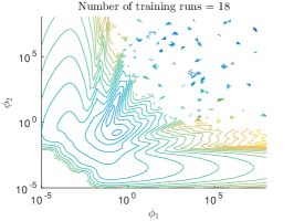
((a)) Numerically unstable surface

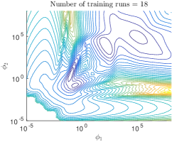
((b)) Numerically stable surface

Figure 3: Projection of the negative log-posterior curves in the two dimensional length-scale space. Adding the nugget $\phi_{\delta}$ results in a numerically stable surface.

To overcome this practical deficiency, a correction term in the covariance matrix can be added in order to preserve diagonal dominancy, that is, we add a nugget hyper-parameter $\boldsymbol{\phi}_{\delta}$ to the covariance such that

$$K_{\delta}=K+\boldsymbol{\phi}_{\delta}\,I,$$ (4.1)

is positive definite. Doing so results in the stochastic simulator

$$y_{i}=\eta(\mathbf{x}_{i})+\sigma^{2}\,\boldsymbol{\phi}_{\delta}.$$ (4.2)

Note that the interpolating quality of the Gaussian process is lost, however, the term $\sigma^{2}\,\boldsymbol{\phi}_{\delta}$ accounts for the variability of the simulator that cannot be explained by the emulator given the original assumptions (adequacy of the covariance function, for example). The nugget can also provide further quantification of model uncertainty in the inference process as it provides an alternative to smoothing an already complex surface. As it is also noticed by Andrianakis and Challenor (2012) and Ranjan et al. (2011), the quality of the emulator changes with the inclusion of the nugget, since it modifies the objective function itself by introducing new modes in the landscape of the posterior distribution. The configuration reflected by new modes in these cases might correspond to emulators with no local dependencies and an overall simple trend, defined from the basis functions and regression hyper-parameters $\boldsymbol{\beta}$. Therefore, if a Gaussian process with no local dependencies, e.g. with its mode farther away from the origin in the length-scale space, is assessed as not appropriate for the model, a regularisation term can be added in the optimisation formulation as in (Andrianakis and Challenor, 2012). This corresponds to precautions for the inclusion of the nugget and can be seen as elicited prior beliefs on the Bayesian formulation. However, by using a multi-modal sampler for stochastic optimisation as the one proposed, a robust emulator capable of mixing various possibilities can be provided. This results in an emulator that is able to cope with violations to the modelling assumptions originated by working with a limited amount of training runs.

We incorporate the nugget term $\boldsymbol{\phi}_{\delta}$ as a hyper-parameter of the correlation function in the Bayesian inference process. As suggested by Ranjan et al. (2011) a uniform prior distribution $U(10^{-12},1)$ for such parameter is considered. The effect of the bounds is twofold. First, the lower bound is used to guarantee stability in the covariance matrix. Second, the upper bound is used to force the numerical noise of the simulator to be smaller than the signal noise of the emulator itself. Note that this last assumption can be omitted if the problem requires it. By considering the correlation matrix as in equation (4.1), this yields

$$\Sigma_{\delta} =\sigma^{2}\,K_{\delta},$$ (4.3)

where $K_{\delta}$ denotes the corrected correlation matrix and $\Sigma_{\delta}$ has been used to denote the covariance matrix of the Gaussian process. By doing so it is clear that previous considerations regarding $\sigma^{2}$, such as the ability of marginalising it as a nuisance parameter and the use of a non-informative prior remain unchanged (De Oliveira, 2007).

5 Numerical Experiments

To illustrate the robustness of estimating the hyper-parameters of a Gaussian process using the parallel AIMS-OPT framework, three test cases have been selected. The first two are common examples that can be found in the literature. The first is known as the Branin function and has been modified to resemble usual properties of engineering applications (Forrester et al., 2008). The second one (Bastos and O’Hagan, 2009) has been used as a two dimensional function with a challenging complexity for emulating purposes. The third example presented in this section comes from a real dataset also presented in Bastos and O’Hagan (2009). In all the examples it is assumed that $h(\mathbf{x})=(1,x_{1},\ldots,x_{p})^{T}$. Regarding the nugget, a sigmoid transformation has been performed in order to sample from a Gaussian distribution. Namely, we sample an auxiliary $z_{\delta}$ as part of the multivariate Gaussian in (3.19), and compute the nugget as

$$\theta_{\delta}=\frac{1-l_{b}}{1+\exp(-z_{\delta})}+l_{b},$$ (5.1)

where $l_{b}$ is the lower bound for the nugget, which is set equal to $10^{-12}$. Additionally, the uniform meta-prior distribution of equation (3.4) has been considered in a practical support of the length-scale parameters in the logarithmic space, namely a uniform distribution with support in $[-7,7]$. For the nugget, a truncated beta distribution with parameters $\alpha=\beta=0.5$ has been considered since it corresponds to a non informative meta-prior in the interval $[l_{b},\,1]$. Here the prefix meta has been used to refer to the algorithm’s prior distribution and to set a clear distinction from the prior used in the modelling assumptions in equation (2.13).

The code has been implemented in MATLAB and all examples have been run in a GNU/Linux machine with an Intel i5 processor with 8 Gb of RAM. For the purpose of reproducibility, the code used to generate the examples is available for download at https://github.com/agarbuno/paims_codes.

5.1 Branin Function

The version of the Branin function used in this paper is a modification made by Forrester et al. (2008) for the purpose of Kriging prediction in engineering applications. It is a rescaled version of the original in order to bound the inputs to the rectangle $[0,1]\times[0,1]$, with an additional term that modifies its landscape to include a global optimum. Namely,

$$f({\bf x})=\left(\overline{x}_{2}-\frac{5.1}{4\pi^{2}}\overline{x}_{1}^{2}+\frac{5}{\pi}\overline{x}_{1}-6\right)^{2}+10\left[\left(1-\frac{1}{8\pi}\right)\cos(\overline{x}_{1})+1\right]+5\overline{x}_{1},$$ (5.2)

where $\overline{x}_{1}=15\,x_{1}-5$ and $\overline{x}_{2}=15\,x_{2}$.

For this case, a sample of 18 design points were chosen with a Latin hypercube sampling scheme. The resulting log-posterior function possesses 4 different modes in its landscape (see Figure 4(a)) leading to 4 possible configurations of the correlation function. Thus, the impact of the training runs used to construct the emulator is evident. Among these modes, 4 different types of emulators can be distinguished: an emulator with high sensitivity to changes in input $x_{1}$ (mode A in Figure 4(a)); an emulator with rapid changes in $x_{2}$ for the correlation structure of the training runs (mode B); a limiting case where dimension $x_{2}$ is disregarded in the correlation function, due to a high value in $\boldsymbol{\phi}_{2}$ (mode C); or a second limiting emulator which approximates a Bayesian linear regression model (mode D) (see Andrianakis and Challenor, 2012, for a detailed discussion).

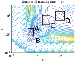
((a)) Level curves and modes

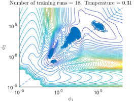
((b)) Parallel AIMS-OPT sample

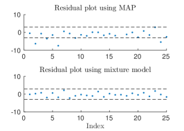
((c)) Residual plots

Figure 4: Projection of the negative log-posterior curves in the two dimensional length-scale space for the Branin simulator. The minimum possible value of $10^{-12}$ for the nugget $\boldsymbol{\phi}_{\delta}$ has been used for such projection. The reference diagonal helps visualise the regions where the length scales favour one dimension over the other.

For this example, two thousand samples were generated in each annealing level. The parallel AIMS-OPT algorithm generated 7 annealing levels to produce the samples in Figure 4(b). The RMSE of the MAP model is 7.068 whereas the RMSE of the mixture is 15.099 which is an indication that in terms of brute prediction, the mixture model could be improved by taking more samples. Figure 4(c) depicts the standardised residuals from both the MAP approach (top) and the mixture model (bottom) using equations (2.10) and (2.11) with uniform weights in the sample. The standardised residuals are defined as

$$r(\mathbf{x})=\frac{y-\mu(\mathbf{x})}{\sqrt{\sigma^{2}(\mathbf{x})}},$$ (5.3)

where $y$ is the output for configuration $\mathbf{x}$, $\mu(\mathbf{x})=E[y|\mathbf{x},\mathcal{D}]$ and $\sigma^{2}(\mathbf{x})=\text{var}(y|\mathbf{x},\mathcal{D})$, the posterior mean and variance for configuration $\mathbf{x}$ (see Bastos and O’Hagan, 2009, for a more detailed discussion on diagnostics). By marginalising the hyper-parameters it is clear that our estimation is a more robust in terms of error prediction. Even with such limited amount of information the residuals suggest that the uncertainty is being incorporated appropriately in the marginalised predictive posterior distribution in equation (2.6). The standardised residuals are inside the 95% confidence bands, assuming approximate normality, though not too close to 0. This is an indicator that although greater variability is expected, excessively large variances are avoided. This is done by means of the integrated predictive distribution and the use of the proposed sampler to build a mixture of emulators leaving the predicted errors inside appropriate bounds.

5.2 2D Model

This function has already been used as an example for emulation purposes and can be found in GEM-SA software web page (http://ctcd.group.shef.ac.uk/gem.html). Even though it is a two dimensional problem it also serves as a good illustration of the importance of estimating the hyper-parameters of a Gaussian process with a multi-modal sampler. The mathematical expression for this simulator is

$$f({\bf x})=\left[1-\exp\left(-\frac{0.5}{x_{2}}\right)\right]\,\left(\frac{2300x_{1}^{3}+1900x_{1}^{2}+2092x_{1}+60}{100x_{1}^{2}+500x_{1}^{2}+4x_{1}+20}\right).$$ (5.4)

As in the previous case, the training runs and the modelling assumptions fail to summarise the uncertainty in a uni-modal posterior distribution. The design points where selected using a Latin hypercube in the rectangle $[0,1]\times[0,1]$. It can be seen from Figure 5(a) that the modes are separated by a wide valley of low posterior probability, which can become an overwhelming task for traditional MCMC samplers. The proposed sampler is able to cope with all local and global spread dynamics present in the neighbourhoods of the modes it encounters, as shown in Figure 5(b).

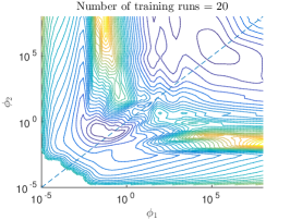
((a)) Level curves with reference prior

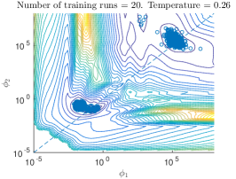
((b)) Parallel AIMS-OPT sample

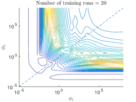
((c)) Level curves with uniform prior

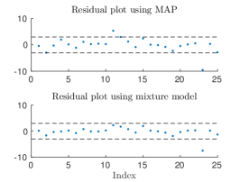
((d)) Residuals plot

Figure 5: Projection of the negative log-posterior curves in the two dimensional length-scale space for the 2D Model simulator. The minimum possible value of $10^{-12}$ for the nugget $\boldsymbol{\phi}_{\delta}$ has been used for such projection. The reference diagonal helps visualise the regions where the length scales favour one dimension over the other.

Depicted in Figures 5(a) and 5(c) the use of the reference prior in the posterior distribution removes probability mass from the neighbourhood around the origin. This validates the use of the reference prior to cut out regions from the space of hyper-parameters for the sampling and exploit the most information contained in the data available, namely, the training runs $\mathcal{D}$. As in the previous example, two thousand samples were generated in each annealing level. The parallel AIMS-OPT algorithm generated 7 annealing levels to produce the samples in Figure 5(b). In terms of prediction accuracy, we now obtain that the RMSE is 1.356 for the MAP estimate and 1.345 for the mixture model. While as for the residuals, we can see from Figure 5(d) that the mixture model allows for a more robust prediction of the error, by means of increasing the variability in particular locations. This can be seen as the standardised residuals are concentrated within the 95% confidence bands of an approximate assumed normality, resulting in a more robust estimation of the error by the use of a mixture model. This motivates the use of multi-modal density samplers in the context of optimisation, where if a single candidate is provided the overall error prediction of the emulator might be biased towards more concentrated predictions around the mean estimation.

5.3 Nilson-Kuusk Model

This simulator is built from the Nilson-Kuusk model for the reflectance for a homogeneous plant canopy. Such model is a five dimensional simulator whose inputs are the solar zenith angle, the leaf area index, relative leaf size, the Markov clumping parameter and a model parameter $\lambda$ (see Nilson and Kuusk, 1989, for further details on the model itself and the meaning of the inputs and outputs). For the analysis presented in this paper a single output emulator is assumed and the set of the inputs have been rescaled to fit the hyper-rectangle $[0,1]^{5}$ on a five dimensional space as in Bastos and O’Hagan (2009).

As in the previous test cases, the design points were chosen by Latin hypercube designs (100 for this case). In this example, the dimension of the problem makes it impossible to plot the level curves of the posterior distribution for the length scale hyper-parameters to visualize potential multiple modes. However, the samples can be visualized by means of a box-plot as shown in Figure 6, where the red line denotes the median, the edges of the box the 25^th and 75^th percentiles, and the whiskers cover the most extreme cases. The samples are obtained after completing 10 levels of the parallel AIMS-OPT algorithm. The box-plots of the approximate optimal solutions strongly suggest that the samples come from a multi-modal posterior distribution. This can be seen from the location of the edges of the boxes and the median for any given input. The last input possesses a very limited spread which might denote a high concentration around one mode. Note that as the magnitude of the length-scale increases, thus reducing the sensitivity of the simulator to such input, the length-scales are located in what can be seen as either a plateau or regions of modes with negligible difference in the posterior density. Additionally, from the range of values that are covered in log-space, it can be noted that the output of the simulator appears to be insensitive to changes of the third and fourth input. Furthermore, a limit-case emulator can be suggested by the box-plot in Figure 6 by considering a surrogate with no third and fourth inputs in the model. Notice the scales for such hyper-parameters in logarithmic space.

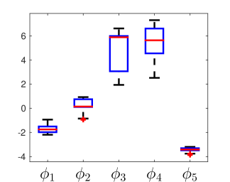
Figure 6: Box-plots of the sample of length-scales obtained by the parallel asymptotically independent Markov sampling.

Due to the larger number of dimensions, five thousand samples were generated for each annealing level. In this case we have that the RMSE of the MAP estimate is 0.022 while the RMSE of the mixture proposal is 0.021 which is a consequence of the posterior distribution being highly concentrated around one mode, in a particular set of length-scales ($\phi_{1},\phi_{2}$ and $\phi_{5}$) while being less specialised for the less sensitive ones ($\phi_{3}$ and $\phi_{4}$). In Figure 7 there is evidence that even with such behaviour the predictive error is improved by narrowing the spread of the standardised residuals, as before, a consequence of an increased estimation of the variability in particular locations. In this case the residuals cannot all be contained in the approximate normality 95% bands but as noted by Bastos and O’Hagan (2009) in their experiments there is strong evidence that more runs of the simulator are needed to adequately built a statistical surrogate. Due to the highly concentrated posterior density around the high sensitive length-scales there seems to be no apparent gain from using the mixture model. However, it can be noted from Figure 6 that by acknowledging the variability of the hyper-parameters, a better understanding of the sensitivity of the simulator with respect to the inputs is achieved. An improved and more robust uncertainty analysis of the simulator can be provided in this case understanding the wide spread of length-scales for particular dimensions. For instance if screening is performed, the MAP estimate will fail to summarise the wide posterior density with respect to $\phi_{3}$ and $\phi_{4}$ and this in turn, will provide partial information. This analysis cannot be performed solely by maximising the posterior density. Therefore the proposed method provides additional insight of the sensitivity of both simulator and emulator.

Figure 7: Residuals plot for the Nilson-Kuusk simulator

6 Conclusions

This paper proposes to estimate the hyper-parameters of a Gaussian process using a new sampler based on the Asymptotically Independent Markov Sampling (AIMS) method. The AIMS-OPT algorithm, used in stochastic optimisation, provides a robust computation of the MAP estimates of the hyper-parameters. This is done by providing a set of approximations to the optimal solution instead of a single approximation as it is so frequently done in the literature. The problem is approached in a combined effort from the computational, optimisation and probabilistic perspectives which serve as solid foundations for building surrogate models for computationally expensive computer codes.

The original AIMS algorithm has been extended to provide an efficient sampler in computational terms, by means of parallelisation, as well as an effective sampler with good mixing qualities, by means of both the delayed rejection and adaptive modification exposed. It has been demonstrated that by using the parallel AIMS-OPT algorithm it is possible to acknowledge uncertainty in the structure of the emulator proposed as illustrated in the examples provided. Structural uncertainty should be taken into account to determine when the training runs available are sufficient to narrow the posterior distribution of the hyper-parameters to a uni-modal convex distribution. Even though it has been proven to be effective in lower and medium dimensional design spaces, research in high dimensional spaces has been left for future research.

Appendix A

In this appendix, a proof that using the delayed rejection algorithm in the AIMS framework leaves the target distribution $p_{k}(\cdot)$ invariant is provided.

A sufficient condition to prove that indeed $p_{k}(\cdot)$ is the stationary distribution for the Markov chain is to prove that the detailed balance condition is satisfied. Since the first stage approval has been proven to satisfy the detailed balance condition in Zuev and Beck (2013), it will only be proved for the second stage sampling.

Let $f_{k}(\boldsymbol{\phi}_{2}|\boldsymbol{\phi}_{0})$ describe the AIMS-OPT delayed transitions in the $k$-th annealing level from $\boldsymbol{\phi}_{0}\rightarrow\boldsymbol{\phi}_{2}$, with $\boldsymbol{\phi}_{2}\neq\boldsymbol{\phi}_{0}$. Let $\boldsymbol{\phi}_{1}$ be the rejected transition in the first stage, for any $\boldsymbol{\phi}_{0},\boldsymbol{\phi}_{1},\boldsymbol{\phi}_{2}\in\Phi\backslash\{\boldsymbol{\phi}_{1}^{(k-1)},\ldots,\boldsymbol{\phi}_{n}^{(k-1)}\}$. It will be proved that for such candidates the following holds:

$$p_{k}(\boldsymbol{\phi}_{0})f_{2}(\boldsymbol{\phi}_{2}|\boldsymbol{\phi}_{0})=p_{k}(\boldsymbol{\phi}_{2})f_{2}(\boldsymbol{\phi}_{0}|\boldsymbol{\phi}_{2}).$$ (A.1)

As seen from the description in section 3.4 it follows that

$$f_{k}(\boldsymbol{\phi}_{2}|\boldsymbol{\phi}_{0}) =\underbrace{\hat{p}_{k,n}(\boldsymbol{\phi}_{1})}_{\text{generate }\boldsymbol{\phi}_{1}}\,\underbrace{(1-a_{1}(\boldsymbol{\phi}_{0},\boldsymbol{\phi}_{1}))}_{\text{reject }\boldsymbol{\phi}_{1}}\,\underbrace{S_{2}(\boldsymbol{\phi}_{2}|\boldsymbol{\phi}_{0},\boldsymbol{\phi}_{1})}_{\text{generate }\boldsymbol{\phi}_{2}}\,\underbrace{a_{2}(\boldsymbol{\phi}_{0},\boldsymbol{\phi}_{2})}_{\text{accept }\boldsymbol{\phi}_{2}},$$ (A.2)

where it is used the fact that AIMS-OPT generates first stage proposals with an independent approximate distribution. Recall that the probability of a second stage proposal is

$$a_{2}(\boldsymbol{\phi}_{0},\boldsymbol{\phi}_{2})=\min\left\{1,\frac{p_{k}(\boldsymbol{\phi}_{2})\,S_{2}(\boldsymbol{\phi}_{0}|\boldsymbol{\phi}_{2},\boldsymbol{\phi}_{1})\,(1-a_{1}(\boldsymbol{\phi}_{2},\boldsymbol{\phi}_{1}))}{p_{k}(\boldsymbol{\phi}_{0})\,S_{2}(\boldsymbol{\phi}_{2}|\boldsymbol{\phi}_{0},\boldsymbol{\phi}_{1})\,(1-a_{1}(\boldsymbol{\phi}_{0},\boldsymbol{\phi}_{1}))}\right\}$$ (A.3)

and the fact that for any two positive numbers $a,b$ the equality $a\,\min\{1,b/a\}=b\,\min\{1,a/b\}$ is satisfied. With these two equalities we can substitute the left hand side of equation (A.1) as

$$p_{k}(\boldsymbol{\phi}_{0})f_{2}(\boldsymbol{\phi}_{2}|\boldsymbol{\phi}_{0}) =\hat{p}_{k,n}(\boldsymbol{\phi}_{1})\,\left[p_{k}(\boldsymbol{\phi}_{0})\,S_{2}(\boldsymbol{\phi}_{2}|\boldsymbol{\phi}_{0},\boldsymbol{\phi}_{1})\,(1-a_{1}(\boldsymbol{\phi}_{0},\boldsymbol{\phi}_{1}))\right]\,a_{2}(\boldsymbol{\phi}_{0},\boldsymbol{\phi}_{2})$$

$$=\hat{p}_{k,n}(\boldsymbol{\phi}_{1})\,\left[p_{k}(\boldsymbol{\phi}_{2})\,S_{2}(\boldsymbol{\phi}_{0}|\boldsymbol{\phi}_{2},\boldsymbol{\phi}_{1})\,(1-a_{1}(\boldsymbol{\phi}_{2},\boldsymbol{\phi}_{1}))\right]\,a_{2}(\boldsymbol{\phi}_{2},\boldsymbol{\phi}_{0})$$

$$=p_{k}(\boldsymbol{\phi}_{2})\,f_{2}(\boldsymbol{\phi}_{0}|\boldsymbol{\phi}_{2}),$$ (A.4)

which proves the detailed balance for the second stage proposal. Note that the proof has been made with no further assumptions about the second stage proposal distribution $S_{2}(\boldsymbol{\phi}_{2}|\boldsymbol{\phi}_{0},\boldsymbol{\phi}_{1})$, as it can be defined from several candidates. In this work, a symmetric proposal that ignores the rejected sample has been used since it can be interpreted as a Random Walk safeguard against a possible ill approximation done by the independent sampler.

References

References

- Andrianakis and Challenor (2012) I. Andrianakis and P. G. Challenor. The effect of the nugget on Gaussian process emulators of computer models. Computational Statistics and Data Analysis, 56(12):4215–4228, 2012.
- Andrianakis and Challenor (2011) Y. Andrianakis and P. G. Challenor. Parameter estimation for Gaussian process emulators. Technical report, Managing Uncertainty in Complex Models, 2011.
- Andrieu et al. (2010) C. Andrieu, A. Doucet, and R. Holenstein. Particle Markov chain Monte Carlo methods. Journal of the Royal Statistical Society. Series B: Statistical Methodology, 72(3):269–342, 2010.
- Bastos and O’Hagan (2009) L. S. Bastos and A. O’Hagan. Diagnostics for Gaussian process emulators. Technometrics, 51(4):425–438, 2009.
- Beck and Zuev (2013) J. Beck and K. M. Zuev. Asymptotically Independent Markov Sampling: a new MCMC scheme for Bayesian Inference. International Journal for Uncertainty Quantification, 3(5), 2013.
- Berger and Bernardo (1992) J. O. Berger and J. M. Bernardo. On the development of reference priors. Bayesian Statistics, 4(4), 1992.
- Berger et al. (1999) J. O. Berger, B. Liseo, and R. L. Wolpert. Integrated likelihood methods for eliminating nuisance parameters. Statistical Science, 14(1):1–28, 1999.
- Berger et al. (2009) J. O. Berger, J. M. Bernardo, and D. Sun. The formal definition of reference priors. Annals of Statistics, 37(2):905–938, 2009.
- Ching and Chen (2007) J. Ching and Y.-C. Chen. Transitional Markov Chain Monte Carlo method for Bayesian model updating, model class selection and model averaging. Journal of Engineering Mechanics, 133(7):816–832, 2007.
- Cressie (1993) N. Cressie. Statistics for Spatial Data. Wiley Series in Probability and Statistics. Wiley, 1993.
- De Oliveira (2007) V. De Oliveira. Objective Bayesian analysis of spatial data with measurement error. Canadian Journal of Statistics, 35(2):283–301, 2007.
- Del Moral et al. (2006) P. Del Moral, A. Doucet, and A. Jasra. Sequential Monte Carlo samplers. Journal of the Royal Statistical Society B, 68(3):411–436, 2006.
- Del Moral et al. (2012) P. Del Moral, A. Doucet, and A. Jasra. On adaptive resampling strategies for sequential Monte Carlo methods. Bernoulli, 18(1):252–278, 2012.
- Draper (1995) D. Draper. Assessment and propagation of model uncertainty. Journal of the Royal Statistical Society, Series B, 57(1):45–97, 1995.
- Fearnhead and Taylor (2013) P. Fearnhead and B. M. Taylor. An adaptive sequential Monte Carlo sampler. Bayesian Analysis, 8(2):411–438, 2013.
- Forrester et al. (2008) A. I. J. Forrester, A. Sóbester, and A. J. Keane. Engineering Design via Surrogate Modelling. 2008.
- Gibbs (1998) M. N. Gibbs. Bayesian Gaussian processes for regression and classification. PhD thesis, Citeseer, 1998.
- Golub and Van Loan (1996) G. Golub and C. Van Loan. Matrix Computations. Johns Hopkins Studies in the Mathematical Sciences. Johns Hopkins University Press, 1996.
- Gramacy and Polson (2009) R. B. Gramacy and N. G. Polson. Particle learning of Gaussian process models for sequential design and optimization. Journal Of Computational And Graphical Statistics, 20(1):18, 2009.
- Haario et al. (2001) H. Haario, E. Saksman, and J. Tamminen. An Adaptive Metropolis Algorithm. Bernoulli, 7(2):223–242, 2001.
- Hankin (2005) R. Hankin. Introducing BACCO, an R bundle for Bayesian analysis of computer code output. Journal of Statistical Software, 14(16), 2005.
- Kalaitzis and Lawrence (2011) A. A. Kalaitzis and N. D. Lawrence. A simple approach to ranking differentially expressed gene expression time courses through Gaussian process regression. BMC bioinformatics, 12:180, Jan. 2011.
- Kennedy and O’Hagan (2001a) M. C. Kennedy and A. O’Hagan. Bayesian calibration of computer models. Journal of the Royal Statistical Society: Series B (Statistical Methodology), 63(3):425–464, Aug. 2001a.
- Kennedy and O’Hagan (2001b) M. C. Kennedy and A. O’Hagan. Supplementary details on Bayesian Calibration of Computer Models. Technical report, 2001b.
- Kirkpatrick et al. (1983) S. Kirkpatrick et al. Optimization by simulated annealing. Journal of statistical physics, 34(5-6):975–986, 1983.
- Liu (2008) J. Liu. Monte Carlo Strategies in Scientific Computing. Springer Series in Statistics. Springer, 2008.
- MacKay (1998) D. J. MacKay. Introduction to Monte Carlo methods. In Learning in graphical models, pages 175–204. Springer, 1998.
- MacKay (1996) D. J. C. MacKay. Hyperparameters: Optimize, or integrate out? Maximum entropy and Bayesian methods, pages 43–59, 1996.
- Mira (2001) A. Mira. On Metropolis-Hastings algorithms with delayed rejection. Metron, 59(3-4):231–241, 2001.
- Neal (1993) R. M. Neal. Probabilistic inference using Markov Chain Monte Carlo methods. Technical Report, pages 1–144, 1993.
- Neal (1996) R. M. Neal. Sampling from multimodal distributions using tempered transitions. Statistics and Computing, 6(4):353–366, 1996.
- Neal (1997) R. M. Neal. Monte Carlo implementation of Gaussian process models for Bayesian regression and classification. Technical Report 9702, 1997.
- Neal (1998) R. M. Neal. Regression and classification using Gaussian process priors. Bayesian Statistics, 6, 1998.
- Neal (2001) R. M. Neal. Annealed importance sampling. Statistics and Computing, 11(2):125–139, 2001.
- Neal (2003) R. M. Neal. Slice sampling. Annals of Statistics, 31(3), 2003.
- Neal (2011) R. M. Neal. MCMC using Hamiltonian dynamics. In Handbook of Markov Chain Monte Carlo. 2011.
- Nilson and Kuusk (1989) T. Nilson and A. Kuusk. A reflectance model for the homogeneous plant canopy and its inversion. Remote Sensing of Environment, 27(2):157–167, 1989.
- Nocedal and Wright (2004) J. Nocedal and S. J. Wright. Numerical Optimization. Springer, 2004.
- Oakley (1999) J. Oakley. Bayesian Uncertainty Analysis for Complex Computer Codes. PhD thesis, 1999.
- Oakley (2002) J. Oakley. Eliciting Gaussian process priors for complex computer codes. Journal of the Royal Statistical Society Series D: The Statistician, 51(1):81–97, 2002.
- Paulo (2005) R. Paulo. Default priors for Gaussian processes. Annals of Statistics, 33(2):556–582, 2005.
- Ranjan et al. (2011) P. Ranjan, R. Haynes, and R. Karsten. A computationally stable approach to Gaussian process interpolation of deterministic computer simulation data. Technometrics, 53(4):366–378, 2011.
- Rasmussen and Williams (2006) C. E. Rasmussen and C. K. I. Williams. Gaussian Processes for Machine Learning. MIT Press, 2006.
- Robert and Casella (2004) C. Robert and G. Casella. Monte Carlo Statistical Methods. Springer Science & Business Media, 2004.
- Schneider and Kirkpatrick (2007) J. Schneider and S. Kirkpatrick. Stochastic Optimization. Scientific Computation. Springer Berlin Heidelberg, 2007.
- Taflanidis and Beck (2008a) A. A. Taflanidis and J. L. Beck. Stochastic Subset Optimization for optimal reliability problems. Probabilistic Engineering Mechanics, 23(2-3):324–338, Apr. 2008a.
- Taflanidis and Beck (2008b) A. A. Taflanidis and J. L. Beck. An efficient framework for optimal robust stochastic system design using stochastic simulation. Computer Methods in Applied Mechanics and Engineering, 198(1):88–101, 2008b.
- Vernon et al. (2010) I. Vernon, M. Goldstein, and R. G. Bower. Galaxy formation: a Bayesian uncertainty analysis. Bayesian Analysis, 5(4):619–669, Dec. 2010.
- Wilkinson (2014) R. D. Wilkinson. Accelerating ABC methods using Gaussian processes. arXiv preprint, 2014.
- Williams and Rasmussen (1996) C. K. I. Williams and C. E. Rasmussen. Gaussian processes for regression. Advances in Neural Information Processing Systems, pages 514–520, 1996.
- Zuev and Beck (2013) K. M. Zuev and J. L. Beck. Global optimization using the Asymptotically Independent Markov Sampling method. Computers & Structures, 126:107–119, Sept. 2013.
- Zuev and Katafygiotis (2011) K. M. Zuev and L. S. Katafygiotis. Modified Metropolis-Hastings algorithm with delayed rejection. Probabilistic Engineering Mechanics, 26(3):405–412, 2011.