Strip maps of small surfaces are convex

Abstract.

The strip map is a natural map from the arc complex of a bordered hyperbolic surface $S$ to the vector space of infinitesimal deformations of $S$. We prove that the image of the strip map is a convex hypersurface when $S$ is a surface of small complexity: the punctured torus or thrice punctured sphere.

1. Introduction

Let $S$ be a compact orientable surface of genus $g\geq 0$ with $p\geq 1$ boundary components, where $2g+p\geq 3$. The arc complex of $S$ is the complex $\overline{X}$ whose vertices are the isotopy classes of non-boundary-parallel embedded arcs in $S$ with endpoints in $\partial S$, and whose $(k-1)$-cells (for $2\leq k\leq 6g-6+3p=:N$) correspond to $k$-tuples of mutually nonisotopic arcs that can be embedded in $S$ disjointly. In this paper we study some realizations of $\overline{X}$ in $\mathbb{R}^{N}$ arising from hyperbolic geometry.

The top-dimensional cells of $\overline{X}$ correspond to so-called hyperideal triangulations of $S$, namely, collections of arcs subdividing $S$ into disks each of which is bounded by three segments of $\partial S$ and three arcs. Elements of $\overline{X}$ can always be represented in barycentric coordinates in the form $\sum_{i=1}^{N}\lambda_{i}\alpha_{i}$ where the $\lambda_{i}$ are nonnegative reals summing to $1$ and the $\alpha_{i}$ are arcs of a hyperideal triangulation. Note that $\overline{X}$ is infinite unless $S$ is the thrice punctured sphere.

A cell of $\overline{X}$ (of any dimension) is called small if the arcs corresponding to its vertices fail to decompose $S$ into disks. For example, vertices of $\overline{X}$ are small cells but top-dimensional cells are not. An important result of Harer and (independently) Penner [3, 6] is the following: the complement $X\subset\overline{X}$ of the union of all small cells is homeomorphic to an open $(N-1)$-ball. Up to boundary effects, we may therefore think of the infinite complex $\overline{X}$ as (essentially) a ball.

It is an interesting question whether this triangulation of the ball can be realized by affine simplices in $\mathbb{R}^{N-1}$ as a tiling of, say, a convex region. One of the main results of [1] is an affirmative answer:

Proposition 1.1.

The projectivized strip map (defined below) associated to a hyperbolic metric on $S$ restricts to an embedding of $X$ into $\mathbb{P}(\mathbb{R}^{N})$, whose image is a convex open set with compact closure in some affine chart.

1.1. The strip map

Let $\mathcal{T}$ be the space of hyperbolic metrics on $S$ with totally geodesic boundary, seen up to isotopy. Then $\mathcal{T}$, also called the Teichmüller space, is diffeomorphic to an open $N$-ball. Let $g\in\mathcal{T}$ be a fixed metric and $x=\sum_{i=1}^{N}\lambda_{i}\alpha_{i}$ a point of $\overline{X}$. We consider for each arc $\alpha\in\overline{X}^{(0)}$ its geodesic representative in $(S,g)$, still denoted $\alpha$, that exits $\partial S$ perpendicularly: in particular, the (representatives of the) $\alpha_{i}$ are disjoint. Suppose moreover that for each $\alpha\in\overline{X}^{(0)}$ we are given a point $p_{\alpha}\in\alpha$, called the waist. To any reals $c_{1}\dots,c_{N}\geq 0$ we can then associate a deformation $\mathsf{Strip}\left(g,\sum_{i=1}^{N}c_{i}\alpha_{i}\right)\in\mathcal{T}$, as follows:

• Glue funnels to $\partial S$, turning $(S,g)$ into an infinite-area hyperbolic surface $S^{\prime}$ without boundary;

• For each $1\leq i\leq N$, cut $S^{\prime}$ open along the geodesic $\alpha_{i}^{\prime}$ that extends $\alpha_{i}$;

• Insert along $\alpha^{\prime}_{i}$ a strip of $\mathbb{H}^{2}$ of width $c_{i}$, i.e. the region bounded by two geodesics of $\mathbb{H}^{2}$ perpendicular to a segment of length $c_{i}$ at its endpoints. Make sure these endpoints become glued to the two copies of the waist $p_{\alpha_{i}}\in\alpha_{i}^{\prime}$ obtained after cutting $\alpha_{i}^{\prime}$ open.

• Define $\mathsf{Strip}\left(g,\sum_{i=1}^{N}c_{i}\alpha_{i}\right)$ as the convex core of the new surface with $N$ strips inserted.

We may now define a continuous map associated to $g\in\mathcal{T}$ and to the chosen system of waists $(p_{\alpha})_{\alpha\in\overline{X}^{(0)}}$:

$$\begin{array}[]{rrcl}\boldsymbol{f}:&\overline{X}&\longrightarrow&T_{[g]}\mathcal{T}\\ &\sum_{1}^{N}\lambda_{i}\alpha_{i}&\longmapsto&\left.\frac{\mathrm{d}}{\mathrm{d}t}\right|_{t=0}\mathsf{Strip}\left(g,\sum_{i=1}^{N}t\lambda_{i}\alpha_{i}\right).\end{array}$$

This map $\boldsymbol{f}$, called the (infinitesimal) strip map, is the main object of interest in this paper. Its projectivization $f:\overline{X}\rightarrow\mathbb{P}(T_{[g]}\mathcal{T})\simeq\mathbb{P}(\mathbb{R}^{N})$ is the projectivized strip map mentioned in Proposition 1.1. The strip construction goes back at least to Thurston [8]; see also [7].

Remarkably, the set $f(X)$ is actually independent of the choices of waists. In fact $f(X)$ coincides with the projectivization of the space of infinitesimal deformations of the hyperbolic metric on $S$ such that all closed geodesics become (in a strict sense) shorter to first order [1]. This has important consequences concerning the structure of the deformation space of Margulis spacetimes (quotients of $\mathbb{R}^{2,1}$ by free groups acting properly discontinuously), and motivates a more detailed study of $\boldsymbol{f}$.

1.2. Convex hypersurfaces

Proposition 1.1 can be rephrased thus: for any two top-dimensional simplices of $\overline{X}$ with vertex lists $(\alpha,\beta_{1},\dots,\beta_{N-1})$ and $(\alpha^{\prime},\beta_{1},\dots,\beta_{N-1})$, there exist reals $A,A^{\prime},B_{1},\dots,B_{N}$ such that

• $(\boldsymbol{f}(\alpha),\boldsymbol{f}(\beta_{1}),\dots,\boldsymbol{f}(\beta_{N-1}))$ is a basis of $\mathbb{R}^{N}$;

• $\displaystyle{A\boldsymbol{f}(\alpha)+A^{\prime}\boldsymbol{f}(\alpha^{\prime})=\sum_{i=1}^{N-1}B_{i}\boldsymbol{f}(\beta_{i})}$;

• $\sum_{i=1}^{N-1}B_{i}>0$ and $A,A^{\prime}>0$.

(The first two conditions already imply that $(A,A^{\prime},B_{1},\dots,B_{N-1})$ are unique up to scaling.) The following conjecture appears in [1]:

Conjecture 1.2.

For an appropriate choice of waists $(p_{\alpha})_{\alpha\in\overline{X}^{(0)}}$, the image of $\boldsymbol{f}|_{X}$ in $T_{[g]}\mathcal{T}$ is a convex hypersurface, with codimension-1 edges looking salient from the origin. In other words (see Figure 1), the numbers $A,A^{\prime},B_{i}$ defined above satisfy the extra condition $\displaystyle{A+A^{\prime}<\sum_{1}^{N}B_{i}}$.

2pt $\boldsymbol{f}(\alpha)$ at -4 74 $\boldsymbol{f}(\alpha^{\prime})$ at 163 73 $\boldsymbol{f}(\beta_{1})$ at 53 31.5 $\boldsymbol{f}(\beta_{2})$ at 84 74 $0$ at 77 1

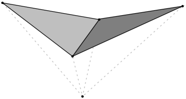
Figure 1. A convex hypersurface in $\mathbb{R}^{3}$.

Since $X$ is dense in $\overline{X}$, restriction to $X$ is inessential in Conjecture 1.2; it is only meant to ensure the image is a (noncomplete) topological submanifold. Conjecture 1.2 would give a realization of $X$ within the simplicial decomposition arising from the convex hull of a discrete set $\boldsymbol{f}(\overline{X}^{(0)})$. It is not clear a priori that such convex realizations should exist, even given Proposition 1.1.

Note that Conjecture 1.2 has a well-studied finite counterpart: the complex of diagonal subdivisions of a (finite, planar, convex) $n$-gon is finite, and is realized as the cell decomposition of the (dual) associahedron, a now classical polytope in $\mathbb{R}^{n-3}$: see for example [5] and the references therein. In this note, we prove

Theorem 1.3.

Conjecture 1.2 is true for $S$ a once punctured torus or a thrice punctured sphere.

The proof will be a rather explicit computation. The once punctured torus and the thrice punctured sphere are called the small (orientable) surfaces; their arc complexes are planar triangle complexes recalled in Section 2.2. As these complexes are dual to trees, it is not hard to realize them in the boundaries of convex (finite or infinite) polyhedra of $\mathbb{R}^{3}$, so Theorem 1.3 is not a new realizability result. However,

• It is interesting to note that the strip map gives a natural realization.

• In the case of the punctured torus, we can extend Theorem 1.3 to singular hyperbolic metrics (Theorem 4.1), replacing the boundary component with a cone point of angle $\theta\in(0,2\pi)$. Proposition 1.1 was already extended to that singular context in [2]. Theorem 4.2 also treats the intermediate case of a cusped metric ($\theta=0$).

• In the case of the thrice punctured sphere, we will see that a naive choice of waists, such as the midpoints of the arcs, does in general not work for Conjecture 1.2. This could shed light on the general case.

1.3. Plan

Section 2 contains reminders about the geometry of strip deformations, the arc complexes of the small surfaces, and hyperbolic geometry (Killing fields and the Minkowski model). Section 3 proves Theorem 1.3 for the thrice punctured sphere, and Section 4 for the once punctured torus.

2. Background

2.1. The sine formula

To estimate the effect of a strip deformation on the metric of $S$, it is convenient to compute how it affects the lengths of various geodesics. Here we give a formula: the proof is similar to the classical cosine formula for earthquake deformations [4], and can be found in [1, §2.1].

For simplicity, we restrict to strip deformations $\boldsymbol{f}(\alpha)$ along a single arc $\alpha$: the general case $\boldsymbol{f}(\sum_{1}^{N}\lambda_{i}\alpha_{i})$ is then recovered by linearity. Let $\gamma\subset S$ be a closed geodesic, and $\mathrm{d}\ell_{\gamma}:T_{[g]}\mathcal{T}\rightarrow\mathbb{R}$ the differential of its length function. Suppose that $\gamma$ intersects $\alpha$ at points $q_{1},\dots,q_{n}$ lying at distances $r_{1},\dots,r_{n}\geq 0$ from the waist $p_{\alpha}$, measured along the arc $\alpha$. Then

(2.1) $$\mathrm{d}\ell_{\gamma}(\boldsymbol{f}(\alpha))=\sum_{i=1}^{n}\sin(\measuredangle_{q_{i}}(\alpha,\gamma))\,\cosh(r_{i})$$

where $\measuredangle_{q_{i}}(\alpha,\gamma)\in(0,\pi)$ denotes the angle, at the point $q_{i}$, between the directions of $\alpha$ and $\gamma$.

This formula shows for example that a strip deformation along a very long arc $\alpha$ will have a huge lengthening effect on the boundary length of $S$ — more precisely, on the lengths of the boundary components of $S$ that $\alpha$ intersects but that lie far away from the waist $p_{\alpha}$.

2.2. Arc complexes of small surfaces

In a (hyperideal) triangulation $\tau$ of the surface $S$, whenever an arc $\alpha$ separates two distinct regions, removing $\alpha$ creates a hyperideal quadrilateral of which $\alpha$ was a diagonal. The triangulation obtained by inserting back the other diagonal is called the diagonal flip of $\tau$ at $\alpha$. Two distinct top-dimensional faces of the arc complex $\overline{X}$ share a codimension-1 face exactly when the two corresponding triangulations of $S$ are related by a diagonal flip.

2.2.1. The thrice punctured sphere

The thrice punctured sphere $S$ has one triangulation $\tau$ obtained by connecting all pairs of distinct punctures together. It also has three more triangulations, obtained from $\tau$ by flipping one of its $3$ edges. In total, the arc complex $\overline{X}$ has $6$ vertices, $9$ one-cells ($3$ of them inner), and $4$ two-cells (the triangulations). The full mapping class group of $S$ has order 12 and projects to the automorphism group of $\overline{X}$, which is the order-6 dihedral group. The kernel is the reflection of $S$ preserving the arcs of $\tau$ pointwise. The dual of $\overline{X}$ is a $3$-branched star. See Figure 2.

2.2.2. The once punctured torus

Up to the action of the mapping class group $\mathrm{GL}_{2}(\mathbb{Z})$, the punctured torus $S$ of interior $\simeq(\mathbb{R}^{2}\smallsetminus\mathbb{Z}^{2})/\mathbb{Z}^{2}$ has only one hyperideal triangulation, obtained e.g. by projecting to $S$ the three segments of $\mathbb{R}^{2}\smallsetminus\mathbb{Z}^{2}$ connecting the origin to $(1,0)$, $(0,1)$, and $(1,1)$. The resulting arc complex $\overline{X}$ is dual to an infinite planar trivalent tree, with one vertex for each rational number $p/q\in\mathbb{P}^{1}(\mathbb{Q})$ (corresponding to the segment from the origin to $(p,q)$). The mapping class group maps onto the automorphism group of $\overline{X}$, with kernel $\{\mathrm{Id},-\mathrm{Id}\}$. See Figure 2.

2pt $\tau$ at 136 96

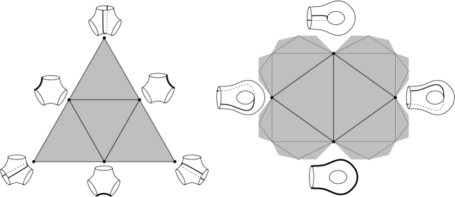
Figure 2. The arc complexes $\overline{X}$ of the two small surfaces.

2.3. Lorentzian geometry

We see $G:=\mathrm{PSL}_{2}(\mathbb{R})$ as the isometry group of the hyperbolic plane $\mathbb{H}^{2}$, and the Lie algebra $\mathfrak{g}:=\mathfrak{psl}_{2}(\mathbb{R})$ as the space of Killing vector fields on $\mathbb{H}^{2}$. The Killing form on $\mathfrak{g}$, multiplied by $\frac{1}{2}$, makes $\mathfrak{g}$ isometric to Minkowski space $(\mathbb{R}^{2,1},\langle\cdot|\cdot\rangle)$. Viewing $\mathbb{H}^{2}$ as one sheet (call it “future”) of the unit hyperboloid of $\mathfrak{g}$, we can then identify the isometry action of $G$ on $\mathbb{H}^{2}$ with the adjoint action. For $\mathcal{Y}\in\mathfrak{g}$, we write $\|\mathcal{Y}\|:=\sqrt{\langle\mathcal{Y}|\mathcal{Y}\rangle}$ and let $d_{\mathbb{H}^{2}}$ be the hyperbolic distance function.

Fact 2.1.

The following are classical:

1. If $\mathcal{Y},\mathcal{Z}\in\mathbb{H}^{2}\subset\mathfrak{g}$ then $\|\mathcal{Y}-\mathcal{Z}\|=2\sinh(d_{\mathbb{H}^{2}}(\mathcal{Y},\mathcal{Z})/2)$.

2. If $\mathcal{Y},\mathcal{Z}\in\mathfrak{g}$ satisfy $\|\mathcal{Y}\|^{2}=\|\mathcal{Z}\|^{2}=1$ and the hyperbolic half-planes $P_{\mathcal{Y}}:=\{u\in\mathbb{H}^{2}\,|~{}\langle u|\mathcal{Y}\rangle\geq 0\}$ and $P_{\mathcal{Z}}:=\{u\in\mathbb{H}^{2}\,|~{}\langle u|\mathcal{Z}\rangle\geq 0\}$ are disjoint, then $\|\mathcal{Y}-\mathcal{Z}\|=2\cosh(d_{\mathbb{H}^{2}}(P_{\mathcal{Y}},P_{\mathcal{Z}})/2)$.

3. If $\mathcal{Y},\mathcal{Z}\in\mathfrak{g}$ are future-pointing lightlike (i.e. isotropic) vectors representing ideal points $y,z\in\partial_{\infty}\mathbb{H}^{2}$, a Killing field $\mathcal{U}\in\mathfrak{g}$ belongs to $\mathbb{R}^{>0}\mathcal{Y}-\mathbb{R}^{>0}\mathcal{Z}$ if and only if $\mathcal{U}$ represents an infinitesimal translation of axis perpendicular to the hyperbolic line $yz$, with $y$ to the left and $z$ to the right of the axis. The velocity of that Killing field along its axis is then just $\|\mathcal{U}\|$.

2.4. Convexity criterion

We can use Killing fields to express the local convexity of the hypersurface $\boldsymbol{f}(X)$ at a codimension-1 face, as follows.

2.4.1. The thrice punctured sphere

For $(S,g)$ a hyperbolic thrice punctured sphere, let $\alpha,\beta,\gamma$ be the arcs of the triangulation $\tau$ of Section 2.2.1 and let $\delta$ be the arc obtained by flipping $\alpha$ in $\tau$.

Note that $(\alpha,\beta,\gamma)$ and $(\beta,\gamma,\delta)$ are top-dimensional faces of the arc complex $\overline{X}$. Let us consider local convexity at the edge $\boldsymbol{f}([\beta,\gamma])=\boldsymbol{f}([\alpha,\beta,\gamma])\cap\boldsymbol{f}([\beta,\gamma,\delta])$, corresponding to the flip that replaces $\alpha$ with $\delta$. By the discussion preceding Conjecture 1.2, there exists a relationship of the form

(2.2) $$B\boldsymbol{f}(\beta)+C\boldsymbol{f}(\gamma)-A\boldsymbol{f}(\alpha)-D\boldsymbol{f}(\delta)=0\in T_{[g]}\mathcal{T}$$

for some $(A,B,C,D)\in\mathbb{R}^{4}\smallsetminus\{0\}$, unique up to scalar multiplication, and we can assume $B+C>0$ and $A,D>0$. Convexity at $\boldsymbol{f}([\beta,\gamma])$ is the property

(2.3) $$A+D<B+C.$$

Lift all arcs $\alpha,\beta,\gamma,\delta$ to $\mathbb{H}^{2}$, obtaining a tiling $\mathcal{E}$ of $\mathbb{H}^{2}$ into infinitely many triangles (or “tiles”), each with one right angle and two hyperideal vertices. This tiling is equivariant with respect to a holonomy representation

$$\rho:\pi_{1}(S)\rightarrow\mathrm{PSL}_{2}(\mathbb{R})\simeq\mathrm{Isom}^{+}(\mathbb{H}^{2}).$$

The relationship (2.2) expresses the fact that appropriate infinitesimal strip deformations on $\beta,\gamma$ can cancel out appropriate infinitesimal strip deformations on $\alpha,\delta$, yielding the trivial deformation of $S$. This can be interpreted (see [1, §4]) as an assignment of a Killing field to each tile, via a map

$$\psi:\mathcal{E}\rightarrow\mathfrak{psl}_{2}(\mathbb{R})\simeq\mathrm{Kill}(\mathbb{H}^{2})$$

satisfying the following properties:

1. Equivariance: for any tile $t\in\mathcal{E}$ and any $\eta\in\pi_{1}(S)$, we have $\psi(\eta\cdot t)=\mathrm{Ad}(\rho(\eta))(\psi(t))$; in other words $\psi$ defines a tilewise Killing field on the quotient $S$ of $\mathbb{H}^{2}$;

2. Vertex consistency: if $t_{1}$, $t_{2}$, $t_{3}$, $t_{4}$ are the tiles adjacent to a lift of the vertex $\alpha\cap\delta$, numbered clockwise, then $\psi(t_{1})-\psi(t_{2})+\psi(t_{3})-\psi(t_{4})=0$; in other words, the $\psi(t_{i})$ form a parallelogram in $\mathfrak{psl}_{2}(\mathbb{R})$;

3. Edge increments: suppose the geodesic line $\lambda$ of $\mathbb{H}^{2}$ is a lift of the arc $\beta$ (resp. $\gamma,\alpha,\delta$), and $p\in\lambda$ is the lift of the corresponding waist. If $\lambda$ separates two adjacent tiles $e,e^{\prime}\in\mathcal{E}$, then $\psi(e^{\prime})-\psi(e)$ is a Killing field representing an infinitesimal translation whose axis is the perpendicular to $\lambda$ through the lifted waist $p$, and whose signed velocity (measured towards $e^{\prime}$) is the real number $B$ (resp. $C,-A,-D$).

The increment condition (iii) expresses the fact that the relative motion of adjacent tiles is given by some strip deformation. The vertex condition (ii) can be rephrased thus: the point $\alpha\cap\delta$ cuts $\alpha$ in two halves, but the increment of $\psi$ across either half is the same. Condition (i) expresses the fact that the linear combination of all 4 (signed) strip deformations is trivial in $T_{[g]}\mathcal{T}$.

We can turn this Killing-field interpretation around:

Criterion 2.2.

Conversely, if we exhibit an assignment $\psi$ of Killing fields to tiles, satisfying (i)–(ii)–(iii) for some reals $A,B,C,D$ with $A,D>0$, then local convexity of $\boldsymbol{f}(\overline{X})$ at the edge $\boldsymbol{f}([\beta,\gamma])$ (where $\boldsymbol{f}$ is defined for the waists induced by the translation axes of the increments of $\psi$) amounts to the inequality (2.3) above: $A+D<B+C$.

In the rest of the paper, we will therefore check convexity of $\boldsymbol{f}$ by exhibiting special Killing fields and computing their velocities $A,B,C,D$.

2.4.2. The once punctured torus

The discussion of Section 2.4.1 is essentially unchanged when $S$ is a hyperbolic once-punctured torus and $\alpha,\beta,\gamma$ the arcs of a triangulation. The only difference is that the tiles are no longer right-angled in general, because $\alpha$ need not intersect its flip $\delta$ perpendicularly (unless $\beta,\gamma$ have equal lengths). This inconvenience is compensated by the fact that $\alpha,\delta$ intersect at their midpoints, which becomes a natural choice of waist.

3. Proof of Theorem 1.3 for the thrice punctured sphere

In this section $S$ is the thrice punctured sphere.

3.1. A bad choice of waists: midpoints

We begin by remarking that, for some hyperbolic metrics $g$ on $S$, picking waists at the midpoints of the arcs would not define a strip map $\boldsymbol{f}:\overline{X}\rightarrow T_{[g]}\mathcal{T}$ with convex image. Indeed, suppose $(S,g)$ has boundary components $a,b,c$ of lengths $0<\ell(a)\ll 1=\ell(b)=\ell(c)$. Let $\alpha,\beta,\gamma,\delta$ denote the the arcs $bc,ca,ab,aa$ respectively, where an arc is referred to by the two boundary components it connects. Then $\ell(\beta)=\ell(\gamma)\gg 1$ and $\ell(\alpha)$ is on the order of $1$: see Figure 3.

2pt $\alpha$ at 201 39 $\beta$ at 115 31 $\gamma$ at 115 64 $\delta$ at 130 54 $p_{\alpha}$ at 202 48 $p_{\beta}$ at 88 30 $p_{\gamma}$ at 88 64 $a$ at -2 50 $b$ at 180 80 $c$ at 180 14

Figure 3. A thrice punctured sphere with a short loop.

We know that there exist reals $A,B,C,D$ with $A,D>0$ satisfying (2.2). By symmetry, we can assume $B=C=1$. Let us prove that $A+D>2=B+C$, in violation of local convexity (2.3).

The Teichmüller space $\mathcal{T}$ is coordinatized by the three boundary lengths $\ell(a),\ell(b),\ell(c)$, hence the range $T_{[g]}\mathcal{T}$ of $\boldsymbol{f}$ admits a dual basis $(\mathrm{d}\ell(a),\mathrm{d}\ell(b),\linebreak\mathrm{d}\ell(c))$. By (2.1), the lengths of $b$ and $c$ are not affected by the infinitesimal deformation $\boldsymbol{f}(\delta)$, because $b\cap\delta=c\cap\delta=\emptyset$. They are affected at roughly unit rate by $\boldsymbol{f}(\alpha)$ because the arc $\alpha$ has length on the order of $1$ and intersects $b,c$. But they are affected at a huge rate by $\boldsymbol{f}(\beta)$ and $\boldsymbol{f}(\gamma)$ because the waists on $\beta$ and $\gamma$ are far away from $b$ and $c$. So the identity $\mathrm{d}\ell(b)(\boldsymbol{f}(\beta)+\boldsymbol{f}(\gamma))=\mathrm{d}\ell(b)(A\boldsymbol{f}(\alpha)+D\boldsymbol{f}(\delta))$, true by (2.2), can only hold if $A$ is itself huge. Thus $A+D>2$, proving that $\boldsymbol{f}$ has nonconvex image.

3.2. A good choice of waists

In a general hyperbolic thrice-punctured sphere $S$, the arcs $\alpha,\delta$ intersect orthogonally (at the midpoint of $\delta$ but not of $\alpha$): we pick this point for the waists $p_{\alpha}$ and $p_{\delta}$, and do the same for the pair formed by $\beta$ (resp. $\gamma$) and its flip. Let us prove that under this choice, $\boldsymbol{f}$ has convex image.

The following is a hyperbolic generalization of a classical Euclidean fact.

Lemma 3.1.

Let $\alpha_{0},\alpha_{1},\alpha_{2}$ be lines in $\mathbb{H}^{2}$ bounding half-planes with disjoint closures in $\mathbb{H}^{2}\cup\partial_{\infty}\mathbb{H}^{2}$ (i.e. the sides of a hyperideal triangle). Let $\beta_{i}$ be the common perpendicular of $\alpha_{i+1}$ and $\alpha_{i-1}$ (indices modulo $3$). The height $h_{i}$ is the common perpendicular to $\beta_{i}$ and $\alpha_{i}$, intersecting $\alpha_{i}$ at the foot $p_{i}$. Then the three heights $h_{i}$ are the inner angle bisectors of the triangle $p_{0}p_{1}p_{2}$.

Proof.

By a compactness argument, there exist points $p^{\prime}_{i}\in\alpha_{i}$ such that the triangle $p^{\prime}_{0}p^{\prime}_{1}p^{\prime}_{2}$ has minimum possible perimeter. By Snell’s law, $\alpha_{i}$ is the outer angle bisector at the vertex $p^{\prime}_{i}$: so it is enough to prove that $p^{\prime}_{i}=p_{i}$.

In Minkowski space $(\mathbb{R}^{2,1},\langle\cdot|\cdot\rangle)$, embed $\mathbb{H}^{2}$ as the upper unit hyperboloid. Let $v_{i}\in\mathbb{R}^{2,1}$ be the unit spacelike vector ($\langle v_{i}|v_{i}\rangle=1$) such that $\langle p^{\prime}_{i+1}|v_{i}\rangle=0=\langle p^{\prime}_{i-1}|v_{i}\rangle$ and $\langle p^{\prime}_{i}|v_{i}\rangle>0$. By symmetry, $\alpha_{i}=\mathrm{ker}\langle\,\cdot\,|v_{i+1}+v_{i-1}\rangle\cap\mathbb{H}^{2}$, and $\mathrm{ker}\langle\,\cdot\,|v_{i+1}-v_{i-1}\rangle\cap\mathbb{H}^{2}$ is the line $h^{\prime}_{i}$ perpendicular to $\alpha_{i}$ at $p^{\prime}_{i}$.

Let $(w_{0},w_{1},w_{2})$ be the dual basis to $(v_{0},v_{1},v_{2})$, i.e. $\langle w_{i}|v_{j}\rangle=\delta_{ij}$. Then $w_{i+1}+w_{i-1}-w_{i}$ pairs to $0$ against $v_{i}+v_{i+1}$ and $v_{i}+v_{i-1}$ and $v_{i+1}-v_{i-1}$. This means that $\alpha_{i-1},\alpha_{i+1}$ and $h^{\prime}_{i}$ have a common perpendicular (necessarily $\beta_{i}$). Therefore $h^{\prime}_{i}=h_{i}$, hence $p^{\prime}_{i}=p_{i}$ as desired. (We may also note that all three heights $h_{i}=h^{\prime}_{i}$ run through the point of $\mathbb{H}^{2}$ collinear with $w_{0}+w_{1}+w_{2}$, since that vector pairs to $0$ against $v_{i+1}-v_{i-1}$.) ∎

We now return to the thrice punctured sphere $S$. Let $\alpha,\beta,\gamma$ be the arcs connecting distinct boundary components; the waists $p_{\alpha},p_{\beta},p_{\gamma}$ are the feet of the heights of the hyperideal triangle with sides $\alpha,\beta,\gamma$. The point $p_{\alpha}=p_{\delta}$ is also the midpoint of the flipped edge $\delta$. Denote by $2\widehat{a},2\widehat{b},2\widehat{c}$ the interior angles of the triangle $p_{\alpha}p_{\beta}p_{\gamma}$ (see Figure 4).

2pt ${}_{\widehat{a}}$ at 73 49 ${}_{\widehat{a}}$ at 93 49 ${}_{\widehat{a}}$ at 74 42 ${}_{\widehat{a}}$ at 92 43 ${}_{\widehat{b}}$ at 46 65 ${}_{\widehat{b}}$ at 55 71 ${}_{\widehat{b}}$ at 110 70 ${}_{\widehat{b}}$ at 119 65 ${}_{\widehat{c}}$ at 48 29 ${}_{\widehat{c}}$ at 56 22 ${}_{\widehat{c}}$ at 108 22 ${}_{\widehat{c}}$ at 118 29 $\alpha$ at 85 75 $\beta$ at 23 62 $\beta$ at 143 62 $\gamma$ at 23 33 $\gamma$ at 143 33 $\delta$ at 33 49 $p_{\alpha}$ at 86 40.5 $p_{\beta}$ at 43 77 $p_{\beta}$ at 122 77 $p_{\gamma}$ at 45 18 $p_{\gamma}$ at 120 18 $\ell_{1}$ at 63 66 $\ell_{2}$ at 103 67 $\ell_{3}$ at 101 26 $\ell_{4}$ at 63 25 $t_{1}$ at 63 80 $t_{2}$ at 103 80 $t_{3}$ at 101 13 $t_{4}$ at 63 13

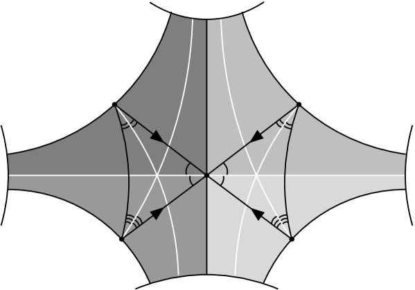
Figure 4. Four colored tiles $t_{1},\dots,t_{4}$ of a 3-punctured sphere $S$, in the universal cover. The white lines are heights. The axes $\ell_{i}$ of all four Killing fields $\psi(t_{i})$ run through $p_{\alpha}$.

The arcs $\beta,\gamma,\alpha,\delta$ subdivide $S$ into four (quotient) tiles $t_{1},t_{2},t_{3},t_{4}$. Each tile $t_{i}$ is a right-angled pentagon containing $p_{\alpha}$ as a vertex, and either $p_{\beta}$ or $p_{\gamma}$ as an interior point of the opposite edge. Let $\ell_{i}\subset t_{i}$ be the segment connecting these two points, oriented towards $p_{\alpha}$. Assign to each tile $t_{i}$ the Killing field $\psi(t_{i})$ defining a unit-velocity infinitesimal translation along $\ell_{i}$. Note that $\psi$ respects the symmetry of $S$ defined by reflection in the edges $\alpha,\beta,\gamma$. We claim that $\psi$ (or strictly speaking, its lift to $\mathbb{H}^{2}$) satisfies the convexity criterion 2.2:

• Equivariance is true by construction of the lift;

• Vertex consistency follows from Lemma 3.1: the points $\psi(t_{1})$,…, $\psi(t_{4})$ form a rectangle in $\mathfrak{psl}_{2}(\mathbb{R})$, hence in particular a parallelogram;

• The local increment $\psi(t)-\psi(t^{\prime})$ across any edge separating tiles $t,t^{\prime}$ is an (infinitesimal) loxodromy of axis perpendicular to $t\cap t^{\prime}$, in the correct direction, passing through the correct waist. Indeed:

  — The increment across (either half of) $\alpha$ is, by symmetry, a translation of velocity $A:=2\cos\widehat{a}$, along an axis perpendicular to $\alpha$ at $p_{\alpha}$, pushing the adjacent tiles towards each other.

  — The increment across (either half of) $\delta$ is a translation of velocity $D:=2\sin\widehat{a}$ along an axis perpendicular to $\delta$ at $p_{\delta}=p_{\alpha}$, pushing the adjacent tiles towards each other.

  — Using symmetry across $\beta$, the increment at the edge $\beta$ is a translation of velocity $B:=2\cos\widehat{b}$ along an axis perpendicular to $\beta$ at $p_{\beta}$, pushing the adjacent tiles away from each other.

  — Similarly, the increment across $\gamma$ is a translation of velocity $C:=2\cos\widehat{c}$ along an axis perpendicular to $\gamma$ at $p_{\gamma}$, pushing the adjacent tiles away from each other.

• The convexity inequality (2.3) to be checked thus becomes $2\cos\widehat{a}+2\sin\widehat{a}<2\cos\widehat{b}+2\cos\widehat{c}$. This holds true: indeed

  $$\cos\widehat{b}+\cos\widehat{c}>1+\cos(\widehat{b}+\widehat{c})>1+\cos(\pi/2-\widehat{a})>\cos\widehat{a}+\sin\widehat{a}$$

  where the first bound is due to concavity of $\cos$, and the second to $\frac{\pi}{2}>\widehat{a}+\widehat{b}+\widehat{c}$ (since $2\widehat{a},2\widehat{b},2\widehat{c}$ are the angles of a hyperbolic triangle).

This proves Theorem 1.3 for the thrice punctured sphere.

4. Proof of Theorem 1.3 for the once punctured torus

In the remainder of the paper, $S$ is a once punctured torus. Let $\alpha,\beta,\gamma$ be the edges of a hyperideal triangulation of $S$, and $\delta$ the edge obtained by flipping $\alpha$.

The waist $p_{\alpha}$ of $\alpha$, still defined as the point $\alpha\cap\delta$, is necessarily fixed under the hyperelliptic involution: $p_{\alpha}$ is now the midpoint of $\alpha$ and of $\delta$.

4.1. Loxodromic commutator

Let $a,b,c,d$ denote the half-lengths of $\alpha,\beta,\gamma,\delta$. Let $S^{\prime}$ denote the surface $S$ extended by a funnel glued along $\partial S$. Place a lift $p$ of $p_{\alpha}=p_{\delta}$ at the center of the projective model of $\mathbb{H}^{2}$ in $\mathbb{P}(\mathbb{R}^{2,1})$. Lifts of the edges $\beta,\gamma$ then define a fundamental domain of $S^{\prime}$, equal to the intersection of $\mathbb{H}^{2}$ with a parallelogram $\Pi$ (Figure 5).

2pt $a$ at 32 44 $a$ at 75 71 $b$ at 39 18 $b$ at 81 18 $b$ at 33 94 $b$ at 71 94 $c$ at 9 74 $c$ at 8 58 $c$ at 104 55 $c$ at 103 39 $d$ at 36 75 $d$ at 80 44 $p$ at 55 50.5 $\Pi$ at 18 18 $[\mathcal{A}]$ at -1 16 $[\mathcal{A}^{\prime}]$ at 110 96 $[\mathcal{D}]$ at 109 16 $[\mathcal{D}^{\prime}]$ at 5 95 $p\mathcal{A}\mathcal{D}$ at 55 38 $p\mathcal{D}\mathcal{A}^{\prime}$ at 85 56 $p\mathcal{A}^{\prime}\mathcal{D}^{\prime}$ at 56 76 $p\mathcal{D}^{\prime}\mathcal{A}$ at 24 57 $\overline{p\mathcal{A}\mathcal{D}}$ at 59 12 $\overline{p\mathcal{D}\mathcal{A}^{\prime}}$ at 117 50 $\overline{p\mathcal{A}^{\prime}\mathcal{D}^{\prime}}$ at 54 98 $\overline{p\mathcal{D}^{\prime}\mathcal{A}}$ at -5 58 ${}_{\mathcal{A}\,\mathrm{sh}\,d-\mathcal{D}\,\mathrm{sh}\,a}$ at 209 33 ${}_{\mathcal{D}\,\mathrm{sh}\,d-\mathcal{A}\,\mathrm{sh}\,a}$ at 207 15 ${}_{\mathcal{D}\,\mathrm{sh}\,a-\mathcal{A}^{\prime}\mathrm{sh}\,d}$ at 237 55 ${}_{\mathcal{A}^{\prime}\mathrm{sh}\,a-\mathcal{D}\,\mathrm{sh}\,d}$ at 279 52 ${}_{\mathcal{A}^{\prime}\mathrm{sh}\,d-\mathcal{D}^{\prime}\mathrm{sh}\,a}$ at 210 81 ${}_{\mathcal{D}^{\prime}\mathrm{sh}\,d-\mathcal{A}^{\prime}\mathrm{sh}\,a}$ at 210 97 ${}_{\mathcal{D}^{\prime}\mathrm{sh}\,a-\mathcal{A}\,\mathrm{sh}\,d}$ at 181 57 ${}_{\mathcal{A}\,\mathrm{sh}\,a-\mathcal{D}^{\prime}\mathrm{sh}\,d}$ at 139 62 $[\mathcal{A}]$ at 153 16 $[\mathcal{A}^{\prime}]$ at 262 96 $[\mathcal{D}]$ at 261 16 $[\mathcal{D}^{\prime}]$ at 159 95

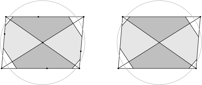
Figure 5. Left: lengths in a fundamental domain (right-angled 8-gon) of the punctured torus $S$ made of 4 tiles in $\mathbb{H}^{2}$. Dark dots in $\mathbb{H}^{2}$ are waists. Right: Killing field assignments in the 8 tiles (abbreviating $\sinh$ to $\mathrm{sh}$ and $\cosh$ to $\mathrm{ch}$).

The boundary of $S$ lifts to lines truncating the corners of $\Pi$. These lines are dual to unit spacelike vectors $\mathcal{A},\mathcal{D},\mathcal{A}^{\prime},\mathcal{D}^{\prime}$ projecting to the vertices of $\Pi$, such that $\alpha\subset\mathrm{span}(\mathcal{A},\mathcal{A}^{\prime})$ and $\delta\subset\mathrm{span}(\mathcal{D},\mathcal{D}^{\prime})$. We may assume that the counterclockwise order of vertics of $\Pi$ goes: $[\mathcal{A}]$, $[\mathcal{D}]$, $[\mathcal{A}^{\prime}]$, $[\mathcal{D}^{\prime}]$. In $\mathbb{R}^{2,1}$, the third ($p$-parallel) coordinates of $\mathcal{A}$, $\mathcal{D}$, $\mathcal{A}^{\prime}$, $\mathcal{D}^{\prime}$ are respectively $\sinh a$, $\sinh d$, $\sinh a$, $\sinh d$; thus

(4.1) $$(\mathcal{A}+\mathcal{A}^{\prime})\sinh d=(\mathcal{D}+\mathcal{D}^{\prime})\sinh a.$$

The lifts of the edges $\alpha,\delta$ subdivide $\Pi\cap\mathbb{H}^{2}$ into four tiles $p\mathcal{A}\mathcal{D}$, $p\mathcal{D}\mathcal{A}^{\prime}$, $p\mathcal{A}^{\prime}\mathcal{D}^{\prime}$, $p\mathcal{D}^{\prime}\mathcal{A}$ (see Figure 5), adjacent respectively to tiles $\overline{p\mathcal{A}\mathcal{D}}$, $\overline{p\mathcal{D}\mathcal{A}^{\prime}}$, $\overline{p\mathcal{A}^{\prime}\mathcal{D}^{\prime}}$, $\overline{p\mathcal{D}^{\prime}\mathcal{A}}$ outside $\Pi$. We pick the following assignment of Killing fields:

$$\psi(p\mathcal{A}\mathcal{D}) := \mathcal{A}\sinh d-\mathcal{D}\sinh a$$

$$\psi(p\mathcal{D}\mathcal{A}^{\prime}) := \mathcal{D}\sinh a-\mathcal{A}^{\prime}\sinh d$$

$$\psi(p\mathcal{A}^{\prime}\mathcal{D}^{\prime}) := \mathcal{A}^{\prime}\sinh d-\mathcal{D}^{\prime}\sinh a$$

$$\psi(p\mathcal{D}^{\prime}\mathcal{A}) := \mathcal{D}^{\prime}\sinh a-\mathcal{A}\sinh d.$$

Note that these are infinitesimal translations whose axes run perpendicular to the sides of $\Pi$, into $\Pi$, because the vectors on the right-hand side belong to the correct 2-plane quadrants by Fact 2.1.(3). We extend $\psi$ by symmetry under the $\pi$-rotations around the waists (midpoints) of $\beta,\gamma$. (This will in particular force each edge increment, such as $\psi(p\mathcal{A}\mathcal{D})-\psi(\overline{p\mathcal{A}\mathcal{D}})$, to have its axis run through the corresponding edge midpoint, i.e. the correct waist.) Note that the $\pi$-rotation around the hyperbolic midpoint of $[\mathcal{A}\mathcal{D}]$, for example, swaps the unit spacelike vectors $\mathcal{A}$ and $\mathcal{D}$, because it swaps the corresponding boundary components of the lift of $S$. This entails

$$\psi(\overline{p\mathcal{A}\mathcal{D}}) := \mathcal{D}\sinh d-\mathcal{A}\sinh a$$

$$\psi(\overline{p\mathcal{D}\mathcal{A}^{\prime}}) := \mathcal{A}^{\prime}\sinh a-\mathcal{D}\sinh d$$

$$\psi(\overline{p\mathcal{A}^{\prime}\mathcal{D}^{\prime}}) := \mathcal{D}^{\prime}\sinh d-\mathcal{A}^{\prime}\sinh a$$

$$\psi(\overline{p\mathcal{D}^{\prime}\mathcal{A}}) := \mathcal{A}\sinh a-\mathcal{D}^{\prime}\sinh d.$$

We may now check the convexity criterion 2.2 for $\psi$. Equivariance is true by construction.

Consistency at the vertex $\alpha\cap\delta$ is the relationship $\psi(p\mathcal{A}\mathcal{D})+\psi(p\mathcal{A}^{\prime}\mathcal{D}^{\prime})=\psi(p\mathcal{D}\mathcal{A}^{\prime})+\psi(p\mathcal{D}^{\prime}\mathcal{A})$, which follows from (4.1) (actually both sides vanish).

The increment at the edge $\beta$, or $\mathcal{A}\mathcal{D}$, is $\psi(p\mathcal{A}\mathcal{D})-\psi(\overline{p\mathcal{A}\mathcal{D}})=(\mathcal{A}-\mathcal{D})(\sinh a+\sinh d)$, an infinitesimal loxodromy with axis perpendicular to $\mathcal{A}\mathcal{D}$ (at the waist), pulling the tile $p\mathcal{A}\mathcal{D}$ away from $\overline{p\mathcal{A}\mathcal{D}}$, i.e. pointing into $\Pi$. By Fact 2.1, its velocity is

$$B:=\|\mathcal{A}-\mathcal{D}\|(\sinh a+\sinh d)=2\cosh b\,(\sinh a+\sinh b).$$

The increment at the edge $\gamma$, or $\mathcal{D}\mathcal{A}^{\prime}$, is $\psi(p\mathcal{D}\mathcal{A}^{\prime})-\psi(\overline{p\mathcal{D}\mathcal{A}^{\prime}})=(\mathcal{D}-\mathcal{A}^{\prime})(\sinh a+\sinh d)$, an infinitesimal loxodromy with axis perpendicular to $\mathcal{D}\mathcal{A}^{\prime}$, pulling $p\mathcal{D}\mathcal{A}^{\prime}$ away from $\overline{p\mathcal{D}\mathcal{A}^{\prime}}$. Its velocity is

$$C:=\|\mathcal{D}-\mathcal{A}^{\prime}\|(\sinh a+\sinh d)=2\cosh c\,(\sinh a+\sinh b).$$

The increment at the edge $\alpha$, or $p\mathcal{A}$, is $\psi(p\mathcal{A}\mathcal{D})-\psi(p\mathcal{D}^{\prime}\mathcal{A})=(\mathcal{A}-\mathcal{A}^{\prime})\sinh d$ (using (4.1)), an infinitesimal loxodromy with axis perpendicular to $\mathcal{A}\mathcal{A}^{\prime}$, pulling $p\mathcal{A}\mathcal{D}$ towards $p\mathcal{D}\mathcal{A}^{\prime}$. Its velocity is

$$A:=\|\mathcal{A}-\mathcal{A^{\prime}}\|\sinh d=2\cosh a\,\sinh d.$$

Finally, the increment at the edge $\delta$, or $p\mathcal{D}$, is $\psi(p\mathcal{D}\mathcal{A}^{\prime})-\psi(p\mathcal{A}\mathcal{D})=(\mathcal{D}-\mathcal{D}^{\prime})\sinh a$ (using (4.1)), an infinitesimal loxodromy with axis perpendicular to $\mathcal{D}\mathcal{D}^{\prime}$, pulling $p\mathcal{D}\mathcal{A}^{\prime}$ towards $p\mathcal{A}\mathcal{D}$. Its velocity is

$$D:=\|\mathcal{D}-\mathcal{D^{\prime}}\|\sinh a=2\cosh d\,\sinh a.$$

It remains to check convexity via (2.3), namely $A+D<B+C$, i.e.

$$\cosh d\,\sinh a+\cosh a\sinh d < (\cosh b+\cosh c)(\sinh a+\sinh d)$$

(4.2) $$\text{i.e. }\hskip 10.0pt\frac{\sinh(a+d)}{\sinh a+\sinh d} < \cosh b+\cosh c.$$

Let us prove (4.2). If $\theta$ denotes the angle formed by the diagonals $\alpha$ and $\delta$ of $\Pi$, then a classical trigonometric formula gives (up to permutation)

$$\cosh(2b) = \sinh a\,\sinh d-\cosh a\,\cosh d\,\cos\theta$$

$$\cosh(2c) = \sinh a\,\sinh d+\cosh a\,\cosh d\,\cos\theta.$$

In particular, $\cosh(2b)+\cosh(2c)$ depends only on $a$ and $d$, not on $\theta$. Since the map $x\mapsto\sqrt{\frac{x+1}{2}}$, taking $\cosh(2u)$ to $\cosh u$, is concave, it follows that the infimal possible value $\mu$ of $\cosh b+\cosh c$ (with $a,d$ fixed) is approached for extremal $\theta$, i.e. when $\{\cosh(2b),\cosh(2c)\}=\{1,2\sinh a\,\sinh d-1\}$: thus $\mu=1+\sqrt{\sinh a\,\sinh d}$. The following are equivalent:

$$\frac{\sinh(a+d)}{\sinh a+\sinh d} < 1+\sqrt{\sinh a\,\sinh d}$$

$$\frac{\sinh a\,(2\sinh^{2}\frac{d}{2})+\sinh d\,(2\sinh^{2}\frac{a}{2})}{\sinh a+\sinh d} < \sqrt{\sinh a\,\sinh d}$$

$$\frac{2\sinh^{2}\frac{d}{2}}{\sinh d}+\frac{2\sinh^{2}\frac{a}{2}}{\sinh a} < \sqrt{\frac{\sinh a}{\sinh d}}+\sqrt{\frac{\sinh d}{\sinh a}}.$$

The last inequality is true: its left hand side is $\tanh\frac{d}{2}+\tanh\frac{a}{2}<2$, while its right hand side is $\geq 2$. This proves convexity, hence Theorem 1.3 for $S$ a one-holed torus.

4.2. Elliptic commutator

Let $g$ be an incomplete hyperbolic metric on the once-punctured torus $S$ whose completion admits a cone singularity of angle $\theta\in(0,2\pi)$. The holonomy representation of $g$ takes the two generators $u,v$ of $\pi_{1}(S)$ to two loxodromics with elliptic commutator. In fact, the fixed points of $[u,v]$, $[v,u^{-1}]$, $[u^{-1},v^{-1}]$, $[v^{-1},u]$ in $\mathbb{H}^{2}$ form the vertices of a convex quadrilateral, equal to a fundamental domain of $(S,g)$ (the generators $u^{\pm 1},v^{\pm 1}$ identify opposite sides in pairs). Any element of the arc complex of $S$ is realized as an embedded geodesic loop $\alpha$ in $S$, connecting the singularity to itself.

We can extend to this context the strip construction along $\alpha$ defined in Section 1.1. The main difference is that there are no funnels to extend the metric $g$ into: instead, we should remove from $(S,g)$ a neighborhood of the puncture $p$, then cut along $\alpha$ and insert an appropriate narrow trapezoid of $\mathbb{H}^{2}$, and finally extend the new metric all the way to a new cone singularity $p^{\prime}$. The position of $p^{\prime}$ is forced by the gluing parameters; see Figure 6.

2pt $\alpha$ at 27 18 $p$ at 38 66 $p^{\prime}$ at 266 74

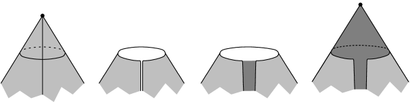
Figure 6. Procedure for inserting a strip into a cone metric along an arc $\alpha$. In $S$, since both endpoints of $\alpha$ are at the singularity $p$, we should actually consider a combination of two such procedures.

The strip map $\boldsymbol{f}$ is therefore still well-defined, valued in the tangent space at the (smooth) point $[g]$ to the representation variety of $\pi_{1}(S)$. Thus Conjecture 1.2 (convexity of $\boldsymbol{f}$) still makes sense, as does the convexity criterion 2.2 (the only difference is that the Killing fields $\psi(\cdot)$ live on the universal cover of the regular part of $S$, which is no longer isometric to $\mathbb{H}^{2}$: but they still make sense as tilewise Killing fields in the quotient $S$).

Theorem 4.1.

Conjecture 1.2 continues to hold for $S$ a punctured torus with cone singularity.

Proof.

We adapt the method from Section 4.1. Let $S$ be a hyperbolic punctured torus with cone singularity. We still call $\alpha,\beta,\gamma$ the edges (running from the singularity to itself) of a triangulation of $S$, and $\delta$ the flip of $\alpha$. The waist of $\alpha$ is its midpoint, where it intersects $\delta$.

Let $a,b,c,d$ denote the half-lengths of $\alpha,\beta,\gamma,\delta$. Place a lift $p$ of $p_{\alpha}=p_{\delta}$ at the center of the projective model of $\mathbb{H}^{2}$ in $\mathbb{P}(\mathbb{R}^{2,1})$. Lifts of the edges $\beta,\gamma$ then define a fundamental domain of $S$, equal to a parallelogram $\Pi\subset\mathbb{H}^{2}$.

Define unit timelike vectors $\mathcal{A},\mathcal{D},\mathcal{A}^{\prime},\mathcal{D}^{\prime}$ projecting to the vertices of $\Pi$, such that $\alpha\subset\mathrm{span}(\mathcal{A},\mathcal{A}^{\prime})$ and $\delta\subset\mathrm{span}(\mathcal{D},\mathcal{D}^{\prime})$. In $\mathbb{R}^{2,1}$, the third ($p$-parallel) coordinates of $\mathcal{A}$, $\mathcal{D}$, $\mathcal{A}^{\prime}$, $\mathcal{D}^{\prime}$ are respectively $\cosh a$, $\cosh d$, $\cosh a$, $\cosh d$; thus

(4.3) $$(\mathcal{A}+\mathcal{A}^{\prime})\cosh d=(\mathcal{D}+\mathcal{D}^{\prime})\cosh a.$$

The lifts of the edges $\alpha,\delta$ subdivide $\Pi$ into four tiles $p\mathcal{A}\mathcal{D}$, $p\mathcal{D}\mathcal{A}^{\prime}$, $p\mathcal{A}^{\prime}\mathcal{D}^{\prime}$, $p\mathcal{D}^{\prime}\mathcal{A}$, adjacent respectively to $\overline{p\mathcal{A}\mathcal{D}}$, $\overline{p\mathcal{D}\mathcal{A}^{\prime}}$, $\overline{p\mathcal{A}^{\prime}\mathcal{D}^{\prime}}$, $\overline{p\mathcal{D}^{\prime}\mathcal{A}}$ (each sharing an edge with $\Pi$). We pick the following assignment of Killing fields (the picture is identical with Figure 5, except $[\mathcal{A}]$, $[\mathcal{D}]$, $[\mathcal{A}^{\prime}]$, $[\mathcal{D}^{\prime}]$ lie inside the disk $\mathbb{H}^{2}$, and $\cosh$ and $\sinh$ are exchanged):

$$\psi(p\mathcal{A}\mathcal{D}) := \mathcal{A}\cosh d-\mathcal{D}\cosh a$$

$$\psi(p\mathcal{D}\mathcal{A}^{\prime}) := \mathcal{D}\cosh a-\mathcal{A}^{\prime}\cosh d$$

$$\psi(p\mathcal{A}^{\prime}\mathcal{D}^{\prime}) := \mathcal{A}^{\prime}\cosh d-\mathcal{D}^{\prime}\cosh a$$

$$\psi(p\mathcal{D}^{\prime}\mathcal{A}) := \mathcal{D}^{\prime}\cosh a-\mathcal{A}\cosh d.$$

Note that these are infinitesimal translations whose axes run perpendicular to the sides of $\Pi$, because the vectors on the right-hand side belong to the correct 2-plane quadrants (Fact 2.1.(3)). We extend $\psi$ by symmetry under the $\pi$-rotations around the waists (midpoints) of $\beta,\gamma$. Note that the $\pi$-rotation around the hyperbolic midpoint of $[\mathcal{A}\mathcal{D}]$, for example, swaps the unit timelike vectors $\mathcal{A}$ and $\mathcal{D}$. This entails

$$\psi(\overline{p\mathcal{A}\mathcal{D}}) := \mathcal{D}\cosh d-\mathcal{A}\cosh a$$

$$\psi(\overline{p\mathcal{D}\mathcal{A}^{\prime}}) := \mathcal{A}^{\prime}\cosh a-\mathcal{D}\cosh d$$

$$\psi(\overline{p\mathcal{A}^{\prime}\mathcal{D}^{\prime}}) := \mathcal{D}^{\prime}\cosh d-\mathcal{A}^{\prime}\cosh a$$

$$\psi(\overline{p\mathcal{D}^{\prime}\mathcal{A}}) := \mathcal{A}\cosh a-\mathcal{D}^{\prime}\cosh d.$$

We may now check the convexity criterion from $\psi$. Equivariance (relative to the holonomy representation of the regular part of $S$) is true by construction. Vertex consistency $\psi(p\mathcal{A}\mathcal{D})+\psi(p\mathcal{A}^{\prime}\mathcal{D}^{\prime})=\psi(p\mathcal{D}\mathcal{A}^{\prime})+\psi(p\mathcal{D}^{\prime}\mathcal{A})$ follows from (4.3).

The increment at the edge $\beta$, or $\mathcal{A}\mathcal{D}$, is $\psi(p\mathcal{A}\mathcal{D})-\psi(\overline{p\mathcal{A}\mathcal{D}})=(\mathcal{A}-\mathcal{D})(\cosh a+\cosh d)$, an infinitesimal loxodromy with axis perpendicular to $\mathcal{A}\mathcal{D}$ (at the waist), pulling the tile $p\mathcal{A}\mathcal{D}$ away from $\overline{p\mathcal{A}\mathcal{D}}$, i.e. pointing into $\Pi$. By Fact 2.1, its velocity is

$$B:=\|\mathcal{A}-\mathcal{D}\|(\cosh a+\cosh d)=2\sinh b\,(\cosh a+\cosh d).$$

The increment at the edge $\gamma$, or $\mathcal{D}\mathcal{A}^{\prime}$, is $\psi(p\mathcal{D}\mathcal{A}^{\prime})-\psi(\overline{p\mathcal{D}\mathcal{A}^{\prime}})=(\mathcal{D}-\mathcal{A}^{\prime})(\cosh a+\cosh d)$, an infinitesimal loxodromy with axis perpendicular to $\mathcal{D}\mathcal{A}^{\prime}$, pulling $p\mathcal{D}\mathcal{A}^{\prime}$ away from $\overline{p\mathcal{D}\mathcal{A}^{\prime}}$. Its velocity is

$$C:=\|\mathcal{D}-\mathcal{A}^{\prime}\|(\cosh a+\cosh d)=2\sinh c\,(\cosh a+\cosh d).$$

The increment at the edge $\alpha$, or $p\mathcal{A}$, is $\psi(p\mathcal{A}\mathcal{D})-\psi(p\mathcal{D}^{\prime}\mathcal{A})=(\mathcal{A}-\mathcal{A}^{\prime})\cosh d$ (using (4.3)), an infinitesimal loxodromy with axis perpendicular to $\mathcal{A}\mathcal{A}^{\prime}$, pulling $p\mathcal{A}\mathcal{D}$ towards $p\mathcal{D}\mathcal{A}^{\prime}$. Its velocity is

$$A:=\|\mathcal{A}-\mathcal{A^{\prime}}\|\cosh d=2\sinh a\,\cosh d.$$

Finally, the increment at the edge $\delta$, or $p\mathcal{D}$, is $\psi(p\mathcal{D}\mathcal{A}^{\prime})-\psi(p\mathcal{A}\mathcal{D})=(\mathcal{D}-\mathcal{D}^{\prime})\cosh a$ (using (4.3)), an infinitesimal loxodromy with axis perpendicular to $\mathcal{D}\mathcal{D}^{\prime}$, pulling $p\mathcal{D}\mathcal{A}^{\prime}$ towards $p\mathcal{A}\mathcal{D}$. Its velocity is

$$D:=\|\mathcal{D}-\mathcal{D^{\prime}}\|\cosh a=2\sinh d\,\cosh a.$$

It remains to check convexity via (2.3), namely $A+D<B+C$, i.e.

$$\sinh d\,\cosh a+\sinh a\cosh d\><\>(\sinh b+\sinh c)(\cosh a+\cosh d)$$

(4.4) $$\text{ i.e. }\hskip 5.0pt\frac{\sinh(a+d)}{\cosh a+\cosh d}=\frac{\sinh\frac{a+d}{2}}{\cosh\frac{a-d}{2}}\><\>\sinh b+\sinh c.$$

Let us prove (4.4). If $\theta$ denotes the angle formed by the diagonals $\alpha$ and $\delta$ of $\Pi$, then a classical trigonometric formula gives (up to permutation)

$$\cosh(2b) = \cosh a\,\cosh d-\sinh a\,\sinh d\,\cos\theta$$

$$\cosh(2c) = \cosh a\,\cosh d+\sinh a\,\sinh d\,\cos\theta.$$

In particular, $\cosh(2b)+\cosh(2c)$ depends only on $a$ and $d$, not on $\theta$. Since the map $x\mapsto\sqrt{\frac{x-1}{2}}$, taking $\cosh(2u)$ to $\sinh u$, is concave, it follows that the infimal possible value of $\sinh b+\sinh c$ (with $a,d$ fixed) is approached when $\theta\rightarrow 0$ or $\theta\rightarrow\pi$, hence $\sinh b+\sinh c\rightarrow\sinh\frac{a+d}{2}+\sinh|\frac{a-d}{2}|$. This is clearly $\geq\left.\sinh\frac{a+d}{2}\right/\cosh\frac{a-d}{2}$ (with equality when $a=d$, but bear in mind that the infimal value is not achieved: $\theta\notin\{0,\pi\}$). Theorem 4.1 is proved. ∎

4.3. Parabolic commutator

Theorem 4.2.

Conjecture 1.2 continues to hold for $S$ a one-cusped torus.

Proof.

The case of a cusp (parabolic commutator) can be recovered as a limit case of an elliptic commutator. Namely, given a one-cusped torus $S$ with arcs $\alpha,\beta,\gamma,\delta$ satisfying the combinatorics above, we can find a fundamental domain in $\mathbb{H}^{2}$ equal to an ideal quadrilateral $\Pi$ whose diagonals intersect at $p$. Denote by $p\mathcal{A}$, $p\mathcal{D}$, $p\mathcal{A}^{\prime}$, $p\mathcal{D}^{\prime}$ the diagonal rays issued from $p$, isometrically parameterized (respectively) by functions $m_{\mathcal{A}}$, $m_{\mathcal{D}}$, $m_{\mathcal{A}^{\prime}}$, $m_{\mathcal{D}^{\prime}}:[0,+\infty)\rightarrow\mathbb{H}^{2}$. Let $H\subset\mathbb{H}^{2}$ be the preimage of a fixed small horoball neighborhood of the cusp. Then there exist reals $\overline{a},\overline{d}>0$ such that $\mathbb{H}^{2}\smallsetminus H$ contains exactly the initial segment $m_{\mathcal{A}}([0,\overline{a}])$ (resp. $m_{\mathcal{D}}([0,\overline{d}])$, $m_{\mathcal{A}^{\prime}}([0,\overline{a}])$, $m_{\mathcal{D}^{\prime}}([0,\overline{d}])$) of the ray $p\mathcal{A}$ (resp. $p\mathcal{D}$, $p\mathcal{A}^{\prime}$, $p\mathcal{D}^{\prime}$).

Given $t>0$, the quadrilateral

$$\Pi_{t}:=\left(m_{\mathcal{A}}(\overline{a}+t)\,,\>m_{\mathcal{D}}(\overline{d}+t)\,,\>m_{\mathcal{A}^{\prime}}(\overline{a}+t)\,,\>m_{\mathcal{D}^{\prime}}(\overline{d}+t)\right)$$

has opposite edges of equal lengths. The isometries taking opposite edges of $\Pi_{t}$ to one another define a representation $\rho_{t}:\pi_{1}(S)\rightarrow\mathrm{PSL}_{2}(\mathbb{R})$ equal to the holonomy of a cone metric converging to the initial cusped metric as $t\rightarrow+\infty$. Let $a_{t},b_{t},c_{t},d_{t}$ be the semi-arc lengths in this cone metric; in particular $a_{t}=\overline{a}+t$ and $d_{t}=\overline{d}+t$.

The member ratio of (4.4) is

$$\frac{\left.\sinh\frac{a_{t}+d_{t}}{2}\right/\cosh\frac{a_{t}-d_{t}}{2}}{\sinh b_{t}+\sinh c_{t}}=\frac{\left.\sinh(\frac{\overline{a}+\overline{d}}{2}+t)\right/\cosh\frac{\overline{a}-\overline{d}}{2}}{\sinh b_{t}+\sinh c_{t}}<1.$$

To prove convexity of the strip map $\boldsymbol{f}$, we only need to bound this ratio away from $1$ (and take limits as $t\rightarrow+\infty$). If $\overline{a}\neq\overline{d}$, this comes from the relationship $\sinh b_{t}+\sinh c_{t}\geq\sinh\frac{a_{t}+d_{t}}{2}+\sinh|\frac{a_{t}-d_{t}}{2}|$ proved at the end of Section 4.2. If $\overline{a}=\overline{d}$, then up to permutation

$$\cosh(2b_{t}) = \cosh^{2}a_{t}-\sinh^{2}a_{t}\,\cos\theta=1+\sinh^{2}a_{t}\,(1-\cos\theta)$$

$$\cosh(2c_{t}) = \cosh^{2}a_{t}+\sinh^{2}a_{t}\,\cos\theta=1+\sinh^{2}a_{t}\,(1+\cos\theta)$$

where $\theta$ is the angle (independent of $t$) formed by the diagonals of $\Pi_{t}$, hence

$$\textstyle{\sinh b_{t}+\sinh c_{t}=\sinh a_{t}\Big{(}\sqrt{\frac{1-\cos\theta}{2}}+\sqrt{\frac{1+\cos\theta}{2}}\,\Big{)}=\sinh a_{t}\,(\sin\frac{\theta}{2}+\cos\frac{\theta}{2}).}$$

Since $\sin\frac{\theta}{2}+\cos\frac{\theta}{2}>1$, this gives the desired bound. ∎

5. Illustration

2pt

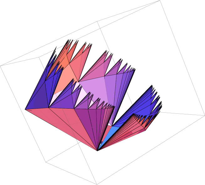
Figure 7.

Figure 7 was made using the Mathematica software. It shows the image of the strip map $\boldsymbol{f}:\overline{X}\rightarrow T_{[g]}\mathcal{T}$ for a hyperbolic torus $(S,g)$ with a cone singularity, composed with a projective transformation $\Phi$ of the range $T_{[g]}\mathcal{T}$ sending the origin to infinity. This composition by $\Phi$ enables us to show the whole set $\boldsymbol{f}(\overline{X})$ (which is unbounded in $T_{[g]}\mathcal{T}$). The plane at infinity was sent by $\Phi$ to the plane containing the tips of all the “teeth”. The gaps between the teeth are not an artefact; they actually grow wider for $g$ a genuine (not conical) hyperbolic metric on $S$. Each triangular gap lies in a plane containing the point $\Phi(0)$ at infinity.

References

- [1] J. Danciger, F. Guéritaud, F. Kassel, Margulis spacetimes via the arc complex, preprint, http://arxiv.org/abs/1407.5422.
- [2] F. Guéritaud, Lengthening deformations of singular hyperbolic tori, to appear in Boileau Festschrift (J.-P. Otal, ed.), Ann. Fac. Sci. Toulouse, available at http://math.univ-lille1.fr/~gueritau/math.html.
- [3] J.L. Harer, The virtual cohomological dimension of the mapping class group of an orientable surface, Invent. Math. 84 (1986), 157–176.
- [4] S.P. Kerckhoff, The Nielsen realization problem, Ann. of Math. 117 (1983), p. 235–265.
- [5] J.-L. Loday, Realization of the Stasheff polytope, Archiv der Mathematik 83–3 (2004), 267–278
- [6] R. C. Penner, The decorated Teichmüller space of punctured surfaces, Comm. Math. Phys. 113 (1987), p. 299–339.
- [7] A. Papadopoulos, G. Théret, Shortening all the simple closed geodesics on surfaces with boundary, Proc. Amer. Math. Soc. 138 (2010), p. 1775–1784.
- [8] W. P. Thurston, Minimal stretch maps between hyperbolic surfaces, preprint (1986), arXiv:9801039.