An Efficient Post-Selection Inference on
High-Order Interaction Models

Abstract

Finding statistically significant high-order interaction features in predictive modeling is important but challenging task. The difficulty lies in the fact that, for a recent applications with high-dimensional covariates, the number of possible high-order interaction features would be extremely large. Identifying statistically significant features from such a huge pool of candidates would be highly challenging both in computational and statistical senses. To work with this problem, we consider a two stage algorithm where we first select a set of high-order interaction features by marginal screening, and then make statistical inferences on the regression model fitted only with the selected features. Such statistical inferences are called post-selection inference (PSI), and receiving an increasing attention in the literature. One of the seminal recent advancements in PSI literature is the works by Lee et al. [1, 2], where the authors presented an algorithmic framework for computing exact sampling distributions in PSI. A main challenge when applying their approach to our high-order interaction models is to cope with the fact that PSI in general depends not only on the selected features but also on the unselected features, making it hard to apply to our extremely high-dimensional high-order interaction models. The goal of this paper is to overcome this difficulty by introducing a novel efficient method for PSI. Our key idea is to exploit the underlying tree structure among high-order interaction features, and to develop a pruning method of the tree which enables us to quickly identify a group of unselected features that are guaranteed to have no influence on PSI. The experimental results indicate that the proposed method allows us to reliably identify statistically significant high-order interaction features with reasonable computational cost.

1 Introduction

Finding statistically reliable high-order interaction features that have significant effects on the response is valuable in many regression problems. For example, in biomedical studies, it is well-known that each genetic factor such as a single gene does not work independently. When a regression analysis is used in biomedical studies for predicting a certain phenotype such as drug response, high-order interactions of multiple genetic factors might be useful [3, 4]. If one has a data set with $d$ original covariates and takes into account interaction terms up to order $r$, the regression model has $\scriptstyle D:=\sum_{\rho=1}^{r}{d\choose\rho}$ features. Unless both $d$ and $r$ are fairly small, the number of features $D$ would be far greater than the sample size $n$. Statistical inferences on such an extremely high-dimensional regression model is quite challenging.

A common practical approach to high-dimensional regression problems is two-stage method, where a subset of features is first selected, and then a regression model only with the selected features is fitted. A statistical issue of such a two-stage method is how to incorporate the effect of the feature selection stage on the statistical inference of the final regression model. If the two stages are performed with the same data set, confidence intervals or $p$-values on the final regression model would be positively biased. Statistical inferences conditional on pre-feature selection is often called post-selection inference (PSI). Until recently, PSI has been recognized to be intractable in most cases because it seems to be difficult to derive the sampling distribution that can fully account for complex feature selection process [5, 6]. Recently, Lee et al. [1, 2] introduced an affirmative solution to PSI for a wide class of feature selection methods. Specifically, they provided a general algorithm for computing an exact sampling distribution of the response conditional on a feature selection event which is represented by a set of affine constraints in the response domain. A notable advantage of their finding is that many commonly used feature selection algorithms such as marginal screening, orthogonal matching pursuit, and Lasso belong to this class. Using the sampling distribution of the response conditional on a feature selection event, one can make various statistical inferences on the post-regression model that properly incorporate the effect of pre-feature selection.

The goal of this paper is to develop a method for finding statistically significant high-order interaction features by using the idea of Lee et al. [1, 2]. Unfortunately, their method cannot be directly applied to our extremely high-dimensional regression model with high-order interaction features. The difficulty lies in the simple fact that a feature selection event in general depends not only on the selected features but also on the unselected features. It suggests that, at least ${\cal O}(D)$ constraints would be needed for characterizing a feature selection event. Since the number of features $D$ is extremely large in our high-order interaction model, it would be computationally intractable to work with all those constrains. In this paper we mainly study PSI on high-order interaction models with marginal screening-based pre-feature selection. In marginal screening, we select top $k$ features from all the $D$ features according to the association of each feature with the response. Despite its simplicity, marginal screening is one of the most-frequently used feature selection methods, and it has been shown to have several desirable statistical properties under some regularity conditions [7, 8, 9, 10]. As we describe in the next section, a feature selection event by marginal screening is characterized by a set of $2k\bar{k}+k$ affine constraints in the response domain, where $\bar{k}:=D-k$ is the number of unselected features. It suggests that the sampling distribution of the response conditional on the marginal screening depends in general on these $2k\bar{k}+k$ affine constraints.

Our main contribution in this paper is to develop a novel algorithm that can efficiently find a subset of these $2k\bar{k}+k$ affine constraints which are guaranteed to have no influence on the conditional sampling distribution. Our basic idea is to exploit the underlying tree structure among a set of high-order interaction features (see Figure 1). Specifically, we derive an efficient pruning condition of the tree such that, for any node in the tree, if a certain condition on the node is satisfied, then all the features corresponding to its descendant nodes are shown to have no influence on the conditional sampling distribution. As demonstrated in the experiment section, our algorithm allows us to work with a PSI for a high-order interaction model e.g., with $d=5000$ and $r=5$ where the number of all the high-order interaction features $D$ is greater than $10^{16}$.

2 Preliminaries

Problem setup

Consider modeling a relationship between a response $Y\in\mathbb{R}$ and $d$-dimensional covariates $\bm{z}=[z_{1},\ldots,z_{d}]^{\top}$ by the following high-order interaction model up to $r^{\rm th}$ order

$$Y=\sum_{j_{1}\in[d]}\alpha_{j_{1}}z_{j_{1}}+\sum_{\begin{subarray}{c}(j_{1},j_{2})\in[d]\times[d]\\ j_{1}\neq j_{2}\end{subarray}}\alpha_{j_{1},j_{2}}z_{j_{1}}z_{j_{2}}+\ldots+\sum_{\begin{subarray}{c}(j_{1},\ldots,j_{r})\in[d]^{r}\\ j_{1}\neq\ldots\neq j_{r}\end{subarray}}\alpha_{j_{1},\ldots,j_{r}}z_{j_{1}}\cdots z_{j_{r}}+\varepsilon,$$ (1)

where $\alpha$s are the coefficients and $\varepsilon$ is a random noise. We assume that each original covariate $z_{j},j\in[d]$ is defined in a domain $[0,1]$ where values 1 and 0 respectively indicate the existence and the non-existence of a certain property, and values between them indicate the “degree” of existence. High-order interaction features thus represent co-existence of multiple properties. For example, if $z_{j_{1}}$ represents high body mass index (BMI) and $z_{j_{2}}$ represents a mutation in a certain gene, we may code these two covariates as

$$z_{j_{1}}:=\left\{\begin{array}[]{ll}1&\text{ if BMI }>30,\\ (\text{BMI}-15)/(30-15)&\text{ if BMI }\in[15,30],\\ 0&\text{ if BMI }<15\end{array}\right.~{}z_{j_{2}}:=\left\{\begin{array}[]{ll}1&\text{ if there is a mutation},\\ 0&\text{ if there is no mutation}.\end{array}\right.$$

Then, an interaction term $z_{j_{1}}z_{j_{2}}$ represents the co-existence of high BMI and a mutation in the gene.

The high-order interaction model (1) has in total $D:=\sum_{\rho\in[r]}{d\choose\rho}$ features. Let us write the mapping from the original covariates $\bm{z}:=[z_{1},\ldots,z_{d}]^{\top}\in\mathbb{R}^{d}$ to the high-order interaction features $\bm{x}:=[x_{1},\ldots,x_{D}]^{\top}\in\mathbb{R}^{D}$ as $\bm{\phi}:[0,1]^{d}\to[0,1]^{D},\bm{z}\mapsto\bm{x},$ where the latter has defined as

$$\bm{x}:=\bm{\phi}(\bm{z})=[z_{1},\ldots,z_{d},z_{1}z_{2},\ldots,z_{d-1}z_{d},\ldots,z_{1}\!\cdot\!\cdot\!\cdot\!z_{k},\ldots,z_{d-k+1}\!\cdot\!\cdot\!\cdot\!z_{d}]^{\top}\in\mathbb{R}^{D}.$$ (2)

Since a high-order interaction feature is a product of original covariates defined in $[0,1]$, the range of each feature $x_{j},j\in[D]$ is also $[0,1]$.

Our goal is to identify statistically significant high-order interaction terms that have large impacts on the response $Y$ by identifying regression coefficients $\alpha$s which are significantly deviated from zero. However, unless both $d$ and $r$ are fairly small, the number of coefficients $\alpha$s to be fitted would be far greater than the sample size $n$, meaning that the unique least-square solution does not exist, and traditional least-square estimation theory cannot be used for making statistical inferences on the fitted model. We thus introduce PSI framework where a subset of features is first selected by marginal screening, and then statistical inferences on the fitted model only with the selected features are considered.

Post-selection inference with marginal screening

In the high-order interaction feature domain $[0,1]^{D}$, we consider the same problem setup as Lee et al.’s work [1, 2]. We assume that the data is generated from the following process

$$\bm{{\cal Y}}\sim N(\bm{\mu},\bm{\Sigma}),$$ (3)

where $\bm{{\cal Y}}\in\mathbb{R}^{n}$ is a random response vector Normally distributed with the mean vector $\bm{\mu}\in\mathbb{R}^{n}$ and the variance-covariance matrix $\bm{\Sigma}\in\mathbb{R}^{n\times n}$. The mean vector $\bm{\mu}$ in general depends on the fixed (non-random) design matrix $\bm{X}\in[0,1]^{n\times D}$. The training set is denoted as $(\bm{X},\bm{y})$ where $\bm{y}\in\mathbb{R}^{n}$ is an observed response from the data generating process (3). The training set is also denoted as $\{(\bm{x}^{i},y^{i})\}_{i\in[n]}$ where $\bm{x}^{i}\in[0,1]^{D}$ is the $i^{\rm th}$ row of $\bm{X}$ and $y_{i}\in\mathbb{R}$ is the $i^{\rm th}$ element of $\bm{y}$. Similarly, the $j^{\rm th}$ column of $\bm{X}$ is denoted as $\bm{x}_{j}$ for $j\in[D]$.

Marginal screening

In the first stage, we select top $k$ features that have strong association with the response. Noting that each feature is defined in $[0,1]$ and the value indicates (the degree of) the existence of a certain property, we consider a score $\bm{x}_{j}^{\top}\bm{y}$ for each of the $D$ features, and select $k$ top features according to their absolute scores $\{|\bm{x}_{j}^{\top}\bm{y}|\}_{j\in[D]}$.

We denote the index set of the selected $k$ features by ${\cal S}$, and that of the unselected $\bar{k}:=D-k$ features by $\bar{{\cal S}}$. As pointed out in [1], marginal screening event is characterized by a set of affine constraints. The fact that $k$ features in ${\cal S}$ are selected and $\bar{k}$ features in $\bar{{\cal S}}$ are not selected is rephrased by

$$|\bm{x}_{j}^{\top}\bm{y}|\geq|\bm{x}_{\ell}^{\top}\bm{y}|\text{ for all }(j,\ell)\in{\cal S}\times\bar{{\cal S}}.$$ (4)

Let $\hat{s}_{j}:={\rm sign}(\bm{x}_{j}^{\top}\bm{y}),j\in{\cal S}$. Then the feature selection event in (4) is rewritten with the sign constraints of the selected features by the following $2k\bar{k}+k$ constraints

$$(-\hat{s}_{j}\bm{x}_{j}-\bm{x}_{\ell})^{\top}\bm{y}\leq 0,~{}(-\hat{s}_{j}\bm{x}_{j}+\bm{x}_{\ell})^{\top}\bm{y}\leq 0,~{}-\hat{s}_{j}\bm{x}_{j}^{\top}\bm{y}\leq 0~{}~{}~{}\forall(j,\ell)\in{\cal S}\times\bar{{\cal S}}.$$ (5)

Since the result of marginal screening depends on the observed response vector $\bm{y}$, we write the feature selection process as a function in the following form

$$\{{\cal S},\bar{{\cal S}},\hat{\bm{s}}\}=\Omega(\bm{y}),$$

where $\hat{\bm{s}}$ is denoted as $\hat{s}_{j}$ for $j\in{\cal S}$. The set of $2k\bar{k}+k$ constraints in (5) is written as $\bm{A}\bm{y}\leq\bm{b}$, for a matrix $\bm{A}\in\mathbb{R}^{(2k\bar{k}+k)\times n}$ and a vector $\bm{b}\in\mathbb{R}^{2k\bar{k}+k}$.

Post-selection inferences

In the second stage, we consider a linear regression model only with the selected features. Let $\bm{X}_{{\cal S}}\in[0,1]^{n\times k}$ be a submatrix of $\bm{X}$ whose columns are indexed by ${\cal S}$. The best linear unbiased estimator of the regression coefficients is the following least-square estimator

$$\hat{\bm{\beta}}_{{\cal S}}:=\bm{X}_{{\cal S}}^{\dagger\top}\bm{y},\text{ where }\bm{X}_{{\cal S}}^{\dagger}:=\bm{X}_{{\cal S}}(\bm{X}_{{\cal S}}^{\top}\bm{X}_{{\cal S}})^{-1}.$$ (6)

The population counterpart of (6) is written as $\bm{{\cal B}}_{{\cal S}}:=\bm{X}_{{\cal S}}^{\dagger\top}\bm{{\cal Y}}.$ Under the data generating process (3), the distribution of $\bm{{\cal B}}_{{\cal S}}$ is written as

$$\bm{{\cal B}}_{{\cal S}}\sim N(\bm{X}_{{\cal S}}^{\dagger\top}\bm{\mu},~{}\bm{X}_{{\cal S}}^{\dagger\top}\bm{\Sigma}\bm{X}_{{\cal S}}^{\dagger})$$ (7)

If the set of features ${\cal S}$ is fixed a priori, then we can make statistical inferences on $\bm{{\cal B}}_{{\cal S}}$ by using the sampling distribution (7). However, if ${\cal S}$ is selected based on $\bm{y}$, the distribution (7) no longer holds. In PSI framework, statistical inferences should be made based on the distribution of $\bm{{\cal B}}_{{\cal S}}$ conditional on the feature selection event $\{{\cal S},\bar{{\cal S}},\hat{\bm{s}}\}=\Omega(\bm{{\cal Y}})$ i.e., we need to have distributional result of the conditional random variable $\bm{X}_{{\cal S}}^{\dagger}\bm{{\cal Y}}~{}\big{|}~{}\{{\cal S},\bar{{\cal S}},\hat{\bm{s}}\}=\Omega(\bm{{\cal Y}}).$

The following theorem presented by Lee et al.[1, 2] enables us to make post-selection inferences as long as the pre-feature selection event is characterized by a set of affine constraints $\bm{A}\bm{y}\leq\bm{b}$.

Theorem 1 (Lee et al. [1, 2]).

Consider a stochastic data generating process $\bm{{\cal Y}}\sim N(\bm{\mu},\bm{\Sigma})$. If a feature selection event is characterized by $\bm{A}\bm{{\cal Y}}\leq\bm{b}$ for an arbitrary matrix $\bm{A}$ and a vector $\bm{b}$ that do not depend on $\bm{{\cal Y}}$, then, for any vector $\bm{\eta}\in\mathbb{R}^{n}$,

$$F_{\bm{\eta}^{\top}\bm{\mu},\bm{\eta}\bm{\Sigma}\bm{\eta}}^{[V^{+}(\bm{A},\bm{b}),V^{-}(\bm{A},\bm{b})]}(\bm{\eta}^{\top}\bm{{\cal Y}})~{}|~{}\bm{A}\bm{{\cal Y}}\leq\bm{b}~{}\sim~{}{\rm Unif}(0,1),$$

where $F_{t,u}^{[v,w]}(\cdot)$ is the cumulative distribution function of the univariate truncated Normal distribution with the mean $t$, the variance $u$, and the lower and the upper truncation points $v$ and $w$, respectively. Furthermore, using $\bm{c}:=\frac{\Sigma\bm{\eta}}{\bm{\eta}^{\top}\Sigma\bm{\eta}}$, the lower and the upper truncation points are given as

$$V^{-}(\bm{A},\bm{b}):=\max_{j:(\bm{A}\bm{c})_{j}<0}\left\{\frac{b_{j}-(\bm{A}\bm{y})_{j}}{(\bm{A}\bm{c})_{j}}\right\}+\bm{\eta}^{\top}\bm{y},~{}V^{+}(\bm{A},\bm{b}):=\min_{j:(\bm{A}\bm{c})_{j}>0}\left\{\frac{b_{j}-(\bm{A}\bm{y})_{j}}{(\bm{A}\bm{c})_{j}}\right\}+\bm{\eta}^{\top}\bm{y}.$$

Theorem 1 indicates that, if we set $\bm{\eta}:=\bm{X}_{{\cal S}}^{\dagger}\bm{e}_{j}$, then the sampling distribution of ${\cal B}_{{\cal S},j}|\{{\cal S},\bar{{\cal S}},\hat{\bm{s}}\}=\Omega(\bm{{\cal Y}})$ is a truncated Normal, where $\bm{e}_{j}$ is a vector of all 0 except 1 in the $j^{\rm th}$ position, and ${\cal B}_{{\cal S},j}$ is the $j^{\rm th}$ element of $\bm{{\cal B}}_{{\cal S}}$. If the lower truncation point $V^{-}(\bm{A},\bm{b})$ and the upper truncation point $V^{+}(\bm{A},\bm{b})$ can be computed, we can make post-selection inferences on each coefficient of the final regression model in the second stage.

However, we cannot handle all the $2k\bar{k}+k$ constraints in $\bm{A}\bm{y}\leq\bm{b}$ because $D$ is exponentially large in our high-order interaction models. In §3, we develop an efficient algorithm by exploiting the underlying tree structure among a set of high-order interaction features that enables us to compute the sampling distribution of $\bm{\eta}^{\top}\bm{{\cal Y}}~{}|~{}\bm{A}\bm{{\cal Y}}\leq\bm{b}$ even when $\bm{A}$ has exponentially large number of rows.

Related works

Before presenting our main contribution, we briefly review related works in the literature. Methods for efficiently finding high-order interaction features and properly evaluating their statistical significances have long been desired in many practical application domains. In the past decade, several authors studied this topic in the context of sparse learning [11, 12, 13]. These methods cannot be used for statistical inferences on the selected features because their main focus is on asymptotic feature selection consistency. In addition, none of these works have special computational trick for handling exponentially large number of interaction features, which makes their empirical evaluations restricted to be only up-to second order interactions. One commonly used heuristic in the context of interaction modeling is to introduce a prior knowledge such as strong heredity assumption [11, 12, 13], where, e.g., an interaction term $z_{1}z_{2}$ would be selected only when both of $z_{1}$ and $z_{2}$ are selected. Such a heuristic restriction is helpful for reducing the number of interaction terms to be considered. However, in many applications, scientists are primarily interested in finding strong interaction features even when their main effects alone do not have any association with the response. The idea of considering a structure among the features and utilizing some pruning rules is common technique in data mining literature [14, 15, 16, 17]. Unfortunately, it is difficult to properly assess the statistical significances of the selected features by these mining techniques.

One traditional approach to assessing the statistical properties on pre-selected features is multiple testing correction (MTC). In the context of DNA microarray studies, many MTC procedures for high-dimensional data have been proposed [18, 19]. An MTC approach for statistical evaluation of high-order interaction features was recently studied in [20, 21]. A main drawback of MTC is that they are highly conservative when the number of candidate features increases. Another common approach is data-splitting (DS). In DS approach, we split the data into two subsets, and use one for feature selection and another for model assessment, which enables us to remove the PSI bias. However, the power of DS approach is clearly weaker than the PSI framework by Lee et al. because only a part of the available sample is used for statistical model assessment. In addition, it is quite annoying that different set of features could be selected if data is splitted differently. Despite two-stage method is frequently used in practical high-dimensional data analysis, proper PSI methods have not been available until recently. Besides the approach by Lee et al.[1, 2], several new directions to PSI have been studied lately [22, 23]. The main contribution of this paper is to develop a practical algorithm for proper statistical assessment of high-order interaction features based on these recent progress on PSI literature.

3 Efficient post-selection inferences for high-order interaction models

In this section we present an efficient algorithm for statistical inferences on high-order interaction model based on post-selection inference framework. The basic idea is to exploit the underlying tree structure among a set of high-order interaction terms as depicted in Figure 1. Using the tree structure we derive a set of pruning conditions of the tree that allows us to efficiently compute the sampling distribution conditional on the marginal screening. even when it is characterized by exponentially large number of affine constraints. In what follows, for any node $j$ in the tree, we let $De(j)$ be the set of all its descendant nodes. In § 3.1, we describe a simple computational trick for marginal screening when there are exponentially large number of high-order interaction features. Then, in § 3.2, we present our main results on efficient post-selection inference for high-order interaction models.

Figure 1: An underlying tree structure among high-order interaction features ($d=4,r=3$).

3.1 Efficient marginal screening for high-order interaction models

In the first marginal screening stage, we select the top $k$ features according to the absolute scores $|\bm{x}_{j}^{\top}\bm{y}|,j\in[D]$. In naive implementation, the absolute scores for all the $D$ features are first computed, and then top $k$ of them are selected. The computational cost of such a naive implementation is ${\cal O}(nD)$, which is computationally intractable for our high-order interaction models. To circumvent the computational cost, we use the following Lemma.

Lemma 2.

Consider high-order interaction feature vectors $\bm{x}_{j}\in[0,1]^{n},j\in[D]$, whose indices are represented in the tree structure depicted in Figure 1. Then, for any node $j\in[D]$ in the tree,

$$|\bm{x}_{\ell}^{\top}\bm{y}|\leq\max\{\sum_{i:y^{i}>0}x^{i}_{j}y^{i},-\sum_{i:y^{i}<0}x^{i}_{j}y^{i}\}~{}~{}~{}\text{ for all }~{}~{}~{}\ell\in De(j),$$ (8)

where $x^{i}_{j}$ is the $(i,j)^{\rm th}$ element of the design matrix $\bm{X}$, i.e., the $i^{\rm th}$ element of the vector $\bm{x}_{j}$.

This simple lemma can be easily proved by noting that, for any $(i,j)\in[n]\times[D]$, $x^{i}_{\ell}\leq x^{i}_{j}\in[0,1]$ for all $\ell\in De(j)$. The lemma has been also used in the context of itemset mining [15, 16, 17].

Lemma 2 suggests that we can exploit the tree structure for efficiently selecting the top $k$ features. In depth first search, if the left-hand-side of (8) in a certain node $j$ is smaller than the $k^{\rm th}$ largest absolute score obtained so far, we can quit searching over its descendant nodes because the lemma indicates that there are no features whose absolute score is greater than the current $k^{\rm th}$ largest one in the subtree.

3.2 Efficient post-selection inference for high-order interaction models

In this section we present our main contribution. As we saw in § 2, a marginal-screening event is represented by $2k\bar{k}+k$ affine constraints. Theorem 1 indicates that a feature selection event characterized by such a set of affine constraints $\bm{A}\bm{y}\leq\bm{b}$ changes the sampling distribution of the post-regression model through the dependencies of the lower and the upper truncation points $V^{-}(\bm{A},\bm{b})$ and $V^{+}(\bm{A},\bm{b})$ on the matrix $\bm{A}$ and the vector $\bm{b}$. Our basic idea is to efficiently identify a subset of affine constraints (a subset of the rows in $\bm{A}$ and the elements in $\bm{b}$) that have no influences on the lower and the upper truncation points by using a set of pruning conditions in the tree structure.

Theorem 3.

Let $\theta\in[2k\bar{k}]$ be the index of the first $2k\bar{k}$ affine constraints in (5), and let ${\cal C}_{1}:=\{1,\ldots,k\bar{k}\}$, and ${\cal C}_{2}:=\{k\bar{k}+1,\ldots,2k\bar{k}\}$. Furthermore, for notational simplicity, assume that first $k$ features are selected and remaining $\bar{k}=D-k$ features are unselected. Then, aside from the sign constraints $\hat{s}_{j}\bm{x}_{j}^{\top}\bm{y}\geq 0,j\in{\cal S}$, a marginal screening event $\bm{A}\bm{y}\leq\bm{b}$ in (5) is written as

$$(\phantom{-}\bm{x}_{\ell(\theta)}-\hat{s}_{j(\theta)}\bm{x}_{j(\theta)})^{\top}\bm{y}\leq 0~{}\text{ with }~{}j(\theta):=\lceil\theta/\bar{k}\rceil,~{}~{}~{}~{}~{}~{}~{}~{}~{}~{}~{}\>\>\ell(\theta):=k+(\theta\bmod\bar{k})~{}\text{ for }~{}\theta\in{\cal C}_{1},$$

$$(-\bm{x}_{\ell(\theta)}-\hat{s}_{j(\theta)}\bm{x}_{j(\theta)})^{\top}\bm{y}\leq 0~{}\text{ with }~{}j(\theta):=\lceil(\theta-k\bar{k})/\bar{k}\rceil,\ell(\theta):=k+(\theta\bmod\bar{k})~{}\text{ for }~{}\theta\in{\cal C}_{2}.$$

Then, the lower and the upper truncation points in Theorem 1 are written as

$$\!\!\!\!\!V^{-}(\bm{A},\bm{b}) =\max\left\{\max_{\begin{subarray}{c}\theta\in[2k\bar{k}]\\ \rho_{j(\theta)}+\bm{x}_{\ell(\theta)}^{\top}\bm{\chi}_{\theta}<0\end{subarray}}\frac{\kappa_{j(\theta)}+\bm{x}_{\ell(\theta)}^{\top}\bm{\xi}_{\theta}}{\rho_{j(\theta)}+\bm{x}_{\ell(\theta)}^{\top}\bm{\chi}_{\theta}},~{}\max_{\begin{subarray}{c}j\in{\cal S}\\ \rho_{j}<0\end{subarray}}\frac{\kappa_{j}}{\rho_{j}}\right\}+\bm{\eta}^{\top}\bm{y},$$ (9a)

$$\!\!\!\!\!V^{+}(\bm{A},\bm{b}) =\min\left\{\min_{\begin{subarray}{c}\theta\in[2k\bar{k}]\\ \rho_{j(\theta)}+\bm{x}_{\ell(\theta)}^{\top}\bm{\chi}_{\theta}>0\end{subarray}}\frac{\kappa_{j(\theta)}+\bm{x}_{\ell(\theta)}^{\top}\bm{\xi}_{\theta}}{\rho_{j(\theta)}+\bm{x}_{\ell(\theta)}^{\top}\bm{\chi}_{\theta}},~{}\min_{\begin{subarray}{c}j\in{\cal S}\\ \rho_{j}>0\end{subarray}}\frac{\kappa_{j}}{\rho_{j}}\right\}+\bm{\eta}^{\top}\bm{y},$$ (9b)

where, for $j\in[D]$ and $\theta\in[2k\bar{k}]$,

$$\kappa_{j}:=\hat{s}_{j}\bm{x}_{j}^{\top}\bm{y},~{}\rho_{j}:=-\hat{s}_{j}\bm{x}_{j}^{\top}\bm{c},~{}\bm{\xi}_{\theta}:=\left\{\begin{array}[]{ll}-\bm{y}&\text{if }\theta\in{\cal C}_{1},\\ \phantom{-}\bm{y}&\text{if }\theta\in{\cal C}_{2},\end{array}\right.~{}\bm{\chi}_{\theta}:=\left\{\begin{array}[]{ll}\phantom{-}\bm{c}&\text{if }\theta\in{\cal C}_{1},\\ -\bm{c}&\text{if }\theta\in{\cal C}_{2},\end{array}\right.$$

with $\bm{c}=\frac{\Sigma\bm{\eta}}{\bm{\eta}^{\top}\Sigma\bm{\eta}}$ as defined before. Furthermore, let

$$a_{j(\theta)}^{+}\!:=\!\!\sum_{i|\xi_{\theta}^{i}>0}\!x_{j(\theta)}^{i}\xi_{\theta}^{i},~{}a_{j(\theta)}^{-}\!:=\!-\!\sum_{i|\xi_{\theta}^{i}<0}\!x_{j(\theta)}^{i}\xi_{\theta}^{i},~{}b_{j(\theta)}^{+}\!:=\!\!\sum_{i|\chi_{\theta}^{i}>0}\!x_{j(\theta)}^{i}\chi_{\theta}^{i},~{}b_{j(\theta)}^{-}\!:=\!-\!\sum_{i|\chi_{\theta}^{i}<0}\!x_{j(\theta)}^{i}\chi_{\theta}^{i},$$

where $\xi_{\theta}^{i}$ and $\chi_{\theta}^{i}$ is the $i^{\rm th}$ element of $\bm{\xi}_{\theta}$ and $\bm{\chi}_{\theta}$, respectively.

For each of the selected feature $j\in{\cal S}$, consider a tree structure as depicted in Figure 1 which only has a set of nodes corresponding to each of the unselected features $\ell\in\bar{{\cal S}}$. Considering a tree for a selected feature $j\in{\cal S}$, if a node corresponding to $\ell(\theta)$, $\theta\in\{\theta|j(\theta)=j\}$ satisfies

$$V^{-}_{\rm best}\geq\left\{\begin{array}[]{ll}-\frac{\kappa_{j(\theta)}-a_{\ell(\theta)}^{-}}{|\rho_{j(\theta)}-b_{\ell(\theta)}^{-}|}+\bm{\eta}^{\top}\bm{y}&\text{if }\rho_{j(\theta)}+b_{\ell(\theta)}^{+}<0,\\ -\frac{\kappa_{j(\theta)}-a_{\ell(\theta)}^{-}}{\max\{|\rho_{j(\theta)}-b_{\ell(\theta)}^{-}|,|\rho_{j(\theta)}+b_{\ell(\theta)}^{+}|\}}+\bm{\eta}^{\top}\bm{y}&\text{otherwise}.\end{array}\right.$$ (12)

then all the constraints indexed by $\theta^{\prime}$ such that $\ell(\theta^{\prime})$ is a descendant of $\ell(\theta)$ in the tree are guaranteed to have no influence on the lower truncation point $V^{-}(\bm{A},\bm{b})$, where $V^{-}_{\rm best}$ is the current maximum of $V^{-}(\bm{A},\bm{b})$ in (9a). Similarly, if

$$V^{+}_{\rm best}\leq\left\{\begin{array}[]{ll}\frac{\kappa_{j(\theta)}-a_{\ell(\theta)}^{-}}{|\rho_{j(\theta)}+b_{\ell(\theta)}^{+}|}+\bm{\eta}^{\top}\bm{y}&\text{if }\rho_{j(\theta)}-b_{\ell(\theta)}^{-}>0,\\ \frac{\kappa_{j(\theta)}-a_{\ell(\theta)}^{-}}{\max\{|\rho_{j(\theta)}-b_{\ell(\theta)}^{-}|,|\rho_{j(\theta)}+b_{\ell(\theta)}^{+}|\}}+\bm{\eta}^{\top}\bm{y}&\text{otherwise}.\end{array}\right.$$ (15)

then all the constraints indexed by $\theta^{\prime}$ such that $\ell(\theta^{\prime})$ is a descendant of $\ell(\theta)$ in the tree are guaranteed to have no influence on the upper truncation point $V^{+}(\bm{A},\bm{b})$, where $V^{+}_{\rm best}$ is the current minimum of $V^{+}(\bm{A},\bm{b})$ in (9b).

The proof is presented in Supplementary Appendix A. Note that (12) and (15) can be evaluated by using information available at the node $\ell(\theta)$. If the conditions in (12) or (15) are satisfied, we can stop searching the tree because it is guaranteed that any constraints indexed by $\theta^{\prime}$ such that $\ell(\theta^{\prime})\in De(\ell(\theta))$ do not have any influences on the truncation point, and hence does not affect the sampling distribution for PSI.

4 Experiments

4.1 Experiments on synthetic data

First, we checked the validity of our post-selection inference algorithm for high-order interaction models by using synthetic data. In the synthetic data experiments, we compared our approach (denoted as PSI: Post-Selection Inference) with ordinary least-squares method (OLS) and data-splitting method (Split). In data splitting method, the data set was randomly divided into two equal-sized subsets, and one of them was used for feature selection, while the other was used for statistical inference on post-regression model.

The synthetic data was generated from $\bm{y}=\bm{X}\bm{\beta}+\bm{\varepsilon},~{}\bm{\varepsilon}\sim N(\bm{0},\sigma^{2}\bm{I}),$ where $\bm{y}\in\mathbb{R}^{n}$ is the response vector, $\bm{X}\in\{0,1\}^{n\times D}$ is the design matrix, and $\bm{\varepsilon}\in\mathbb{R}^{n}$ is the Gaussian noise vector. Here, we did not actually compute the extremely wide design matrix $\bm{X}$ because it has exponentially large number of columns. Instead, we generated a random binary matrix $\bm{Z}\in\{0,1\}^{n\times d}$ and each expanded high-order interaction feature $x^{i}_{j}$ was generated from the $i^{\rm th}$ row of $\bm{Z}$ only when it was needed. For simplicity and computational efficiency, we assumed that the covariates (hence interaction features as well) are binary, and the sparsity rate $\eta\in[0,1]$ (the rate of zeros in the entries of $\bm{Z}$) was changed to see how sparsity is useful for efficient computation. As the baseline, the rest of the parameters were set as $n=100$, $d=100$, $\eta=0.5$, $\sigma=0.1$, $r=3$, $k=10$, and significance level $\alpha=0.05$.

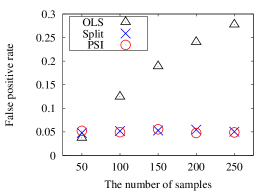
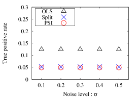
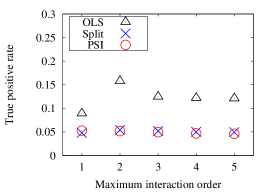
(a) $n\in\{50,\cdots,250\}$	(b) $\sigma\in\{0.1,\cdots,0.5\}$	(c) $r\in\{1,\cdots,5\}$

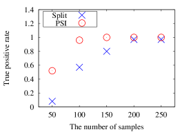
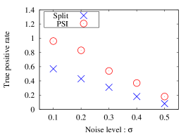
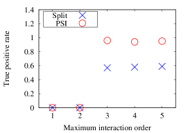
Figure 2: False positive rates of three methods PSI, OLS and Split.

(a) $n\in\{50,\cdots,250\}$	(b) $\sigma\in\{0.1,\cdots,0.5\}$	(c) $r\in\{1,\cdots,5\}$

Figure 3: True positive rates of PSI and Split.

False positive rate control

First, to check whether the methods can properly control the desired false positive rate, we generated data sets with $\bm{\beta}=\mathbf{0}$ and see how many false positives would be reported by each of the three methods. Figure 3 shows the false positive rate defined as $k^{\prime}/k$ where $k^{\prime}$ is the number of features reported as positives in post-regression models. The plots in Figure 3 are the averages over 1000 different trials for various sample size $n\in\{50,\cdots,250\}$, noise level $\sigma\in\{0.1,\cdots,0.5\}$, and maximum interaction order $r\in\{1,\cdots,5\}$. As expected, OLS could not properly control the false positive rates because statistical inferences on the post-regression models would be positively biased when the features were selected by using the same data set. On the other hand, PSI and Split could keep the false positive rates as desired $\alpha=0.05$ level.

True positive rate comparison

Next, we compared true positive rates of PSI and Split. We set all the coefficient as 0 except $\beta_{j}=1$ for $j^{\rm th}$ feature corresponding to the $3^{\rm rd}$ order interaction term $z_{1}z_{2}z_{3}$. In Figure 3, we report the true positive rates for various parameters,which are defined as the number of times when the feature $z_{1}z_{2}z_{3}$ was detected as positive over the number of entire trials. In almost all cases, we see that PSI has larger true positive rates than Split. This is reasonable because the sample size used in the post-selection inference in the latter was half of the former.

Computational efficiency

Finally, we demonstrate the computational efficiency of the proposed method. In Tables 3 and 3, we show the average computation times on 10 trials in seconds and $1-$pruning rates for tree traversing with various those parameters. Although the computation time increases with $d,~{}r$ and $1-\eta$, the computation times were still in acceptable range.

Table 1: Computation times [sec] and $1-$pruning rates ($r=3$).

$d$	Time ($\eta=0.9$)	Time ($\eta=0.7$)	$1-$ pruning rate ($\eta=0.9$)	$1-$ pruning rate ($\eta=0.7$)
100	0.01(0.002)	0.01(0.007)	$1.29\times 10^{-2}(3.42\times 10^{-3})$	$1.76\times 10^{-2}(1.08\times 10^{-2})$
500	0.08(0.02)	0.16(0.11)	$9.71\times 10^{-4}(2.63\times 10^{-4})$	$1.79\times 10^{-3}(1.30\times 10^{-3})$
1000	0.19(0.05)	0.52(0.37)	$2.91\times 10^{-4}(9.77\times 10^{-5})$	$7.11\times 10^{-4}(5.49\times 10^{-4})$
5000	1.03(0.33)	3.36(2.92)	$1.18\times 10^{-5}(3.73\times 10^{-6})$	$3.67\times 10^{-5}(3.28\times 10^{-5})$
10000	2.70(1.09)	9.50(9.20)	$4.12\times 10^{-6}(1.45\times 10^{-6})$	$1.39\times 10^{-5}(1.32\times 10^{-5})$

Table 2: Computation times and $1-$pruning rates ($d=5000$).

$r$	Time ($\eta=0.9$)	Time ($\eta=0.7$)	$1-$ pruning rate ($\eta=0.9$)	$1-$ pruning rate ($\eta=0.7$)
1	0.03(0.001)	0.03(0.001)	$1(0)$	$1(0)$
2	1.01(0.32)	2.59(2.23)	$1.96\times 10^{-2}(6.23\times 10^{-3})$	$5.20\times 10^{-2}(4.54\times 10^{-2})$
3	1.05(0.33)	3.24(2.78)	$1.18\times 10^{-5}(3.73\times 10^{-6})$	$3.67\times 10^{-5}(3.28\times 10^{-5})$
4	1.04(0.33)	3.98(3.00)	$9.47\times 10^{-9}(2.99\times 10^{-9})$	$4.03\times 10^{-8}(3.39\times 10^{-8})$
5	1.03(0.32)	4.17(3.35)	$9.48\times 10^{-12}(2.99\times 10^{-12})$	$4.04\times 10^{-11}(3.39\times 10^{-11})$

Table 3: The number of features reported as positives and computation times [sec].

Dataset	Split			PSI			time of
	1st	2nd	3rd	1st	2nd	3rd	PSI
Communities&Crime09 ($d=253$)	1			2			$1.48$
Communities&Crime11 ($d=289$)		2		3	2	1	$1.46$
BlogFeedback ($d=339$)		2	1	4	12	13	$2.17$
SliceLocalization ($d=769$)		2	28		1	29	$26.33$
UJIIndoorLoc ($d=1053$)	3	4		5	4	1	$4.29$

4.2 Experiments on real data

Here we show the statistical power of PSI and Split in real data. Since the true positive features in real data are unknown, we show the number of features reported as positives in post-regression models assuming that these two methods can properly control false positive rates as we confirmed in synthetic data experiments. We obtained datasets from UCI data repository, which listed in the first column of Table 3. Continuous covariates in the original datasets were first standardized to have the mean zero and the variance one, and then represented the covariate by two binary variables, each of which indicates whether the value is greater than 1 or the value is smaller than -1. We estimated the $\sigma$ in the same way as [1]. We set the maximum interaction order as $r=3$ and the number selected features by marginal screening as $k=30$. For simplicity and computational efficiency, we randomly sampled 1000 instances from each dataset. Table 3 shows the number of features reported as positives on PSI and Split. In almost all cases, PSI found more positive features than Split, while the computational cost of PSI were still in acceptable range.

5 Conclusions

In this paper we proposed an efficient PSI on high-order interaction models with marginal screening-based pre-feature selection. Our key idea is to derive a pruning condition of the tree that quickly identifies a set of unrelated features with PSI. The experimental results indicated that the proposed method allows us to reliably identify statistically significant high-order interaction features with reasonable computational cost.

Appendix A Proof of Theorem 3

In this appendix we prove Theorem 3.

Proof of Theorem 3.

We only show the lower truncation point part of the Theorem. Consider an arbitrary pair $(\theta,\theta^{\prime})\in[2k\bar{k}]^{2}$ such that $j(\theta)=j(\theta^{\prime})$ and $\ell(\theta^{\prime})\in De(\ell(\theta))$. We first note that the fact that $x^{i}_{\ell(\theta^{\prime})}\leq x^{i}_{\ell(\theta)}$ for all $i\in[n]$ indicates that

$$0\leq a^{+}_{\ell(\theta^{\prime})}\leq a^{+}_{\ell(\theta)},~{}0\leq a^{-}_{\ell(\theta^{\prime})}\leq a^{-}_{\ell(\theta)},~{}0\leq b^{+}_{\ell(\theta^{\prime})}\leq b^{+}_{\ell(\theta)},~{}0\leq b^{-}_{\ell(\theta^{\prime})}\leq b^{-}_{\ell(\theta)}$$ (16)

(i) First we prove the first case in (12). Using the relations in 16, we have

$$\rho_{j(\theta^{\prime})}+\bm{x}_{\ell(\theta^{\prime})}^{\top}\bm{\chi}_{\theta^{\prime}}=\rho_{j(\theta^{\prime})}+b^{+}_{j(\theta^{\prime})}-b^{-}_{j(\theta^{\prime})}\leq\rho_{j(\theta)}+b^{+}_{j(\theta)},$$ (17)

where we used $\rho_{j(\theta^{\prime})}=\rho_{j(\theta)}$. Next, when $\rho_{j(\theta^{\prime})}+\bm{x}_{\ell(\theta^{\prime})}^{\top}\bm{\chi}_{\theta^{\prime}}<0$,

$$\frac{\kappa_{j(\theta^{\prime})}+\bm{x}_{\ell(\theta^{\prime})}^{\top}\bm{\xi}_{\theta^{\prime}}}{\rho_{j(\theta^{\prime})}+\bm{x}_{\ell(\theta^{\prime})}^{\top}\bm{\chi}_{\theta^{\prime}}}=\frac{\kappa_{j(\theta^{\prime})}+a^{+}_{\ell(\theta^{\prime})}-a^{-}_{\ell(\theta^{\prime})}}{\rho_{j(\theta^{\prime})}+b^{+}_{\ell(\theta^{\prime})}-b^{-}_{\ell(\theta^{\prime})}}\leq-\frac{\kappa_{j(\theta^{\prime})}-a^{-}_{\ell(\theta^{\prime})}}{|\rho_{j(\theta^{\prime})}-b^{-}_{\ell(\theta^{\prime})}|}\leq-\frac{\kappa_{j(\theta)}-a^{-}_{\ell(\theta)}}{|\rho_{j(\theta)}-b^{-}_{\ell(\theta)}|},$$ (18)

where we used the fact that the numerator is non-negative, and the denominator is non-positive in the left-most fraction. From (17) and (18), we have

$$\rho_{j(\theta)}+b^{+}_{j(\theta)}<0\text{ and }-\frac{\kappa_{j(\theta)}-a^{-}_{\ell(\theta)}}{|\rho_{j(\theta)}-b^{-}_{\ell(\theta)}|}+\bm{\eta}^{\top}\bm{y}\leq V^{-}_{\rm best}~{}\Rightarrow~{}\frac{\kappa_{j(\theta^{\prime})}+\bm{x}_{\ell(\theta^{\prime})}^{\top}\bm{\xi}_{\theta^{\prime}}}{\rho_{j(\theta^{\prime})}+\bm{x}_{\ell(\theta^{\prime})}^{\top}\bm{\chi}_{\theta^{\prime}}}+\bm{\eta}^{\top}\bm{y}\leq V^{-}_{\rm best},$$

which proves the first case in (12). (ii) Next, we prove the second case of (12). When we do not know the sign of the denominator $\rho_{j(\theta^{\prime})}+\bm{x}_{\ell(\theta^{\prime})}^{\top}\bm{\chi}_{\theta^{\prime}}$, we can obtain a slightly loose bound in the following form

$$\begin{split}\frac{\kappa_{j(\theta^{\prime})}+\bm{x}_{\ell(\theta^{\prime})}^{\top}\bm{\xi}_{\theta^{\prime}}}{\rho_{j(\theta^{\prime})}+\bm{x}_{\ell(\theta^{\prime})}^{\top}\bm{\chi}_{\theta^{\prime}}}=\frac{\kappa_{j(\theta^{\prime})}+a^{+}_{\ell(\theta^{\prime})}-a^{-}_{\ell(\theta^{\prime})}}{\rho_{j(\theta^{\prime})}+b^{+}_{\ell(\theta^{\prime})}-b^{-}_{\ell(\theta^{\prime})}}&\leq-\frac{\kappa_{j(\theta^{\prime})}-a^{-}_{\ell(\theta^{\prime})}}{\max\{|\rho_{j(\theta^{\prime})}-b^{-}_{\ell(\theta^{\prime})}|,|\rho_{j(\theta^{\prime})}+b^{+}_{\ell(\theta^{\prime})}|\}}\\ &\leq-\frac{\kappa_{j(\theta)}-a^{-}_{\ell(\theta)}}{\max\{|\rho_{j(\theta)}-b^{-}_{\ell(\theta)}|,|\rho_{j(\theta)}+b^{+}_{\ell(\theta)}|\}}.\end{split}$$ (19)

From (19),

$$-\frac{\kappa_{j(\theta)}-a^{-}_{\ell(\theta)}}{\max\{|\rho_{j(\theta)}-b^{-}_{\ell(\theta)}|,|\rho_{j(\theta)}+b^{+}_{\ell(\theta)}|\}}+\bm{\eta}^{\top}\bm{y}\leq V^{-}_{\rm best}~{}\Rightarrow~{}\frac{\kappa_{j(\theta^{\prime})}+\bm{x}_{\ell(\theta^{\prime})}^{\top}\bm{\xi}_{\theta^{\prime}}}{\rho_{j(\theta^{\prime})}+\bm{x}_{\ell(\theta^{\prime})}^{\top}\bm{\chi}_{\theta^{\prime}}}+\bm{\eta}^{\top}\bm{y}\leq V^{-}_{\rm best},$$

which proves the second case of (12). Combining (i) and (ii), we showed that, if (12) is satisfied for a certain $\theta$, then any constraints indexed by $\theta^{\prime}$ such that $j(\theta^{\prime})=j(\theta)$ and $\ell(\theta^{\prime})\in De(\ell(\theta))$ are guaranteed to have no influence on the lower truncation point $V^{-}(\bm{A},\bm{b})$. The upper truncation point part of the Theorem can be shown similarly. ∎

References

- [1] J. D. Lee and J. E. Taylor. Exact post model selection inference for marginal screening. In Advances in Neural Information Processing Systems, 2014.
- [2] J. D. Lee, D. L. Sun, Y. Sun, and J. E. Taylor. Exact post-selection inference with applications to the LASSO. arXiv:1311.6238v5, 2015.
- [3] Teri A Manolio and Francis S Collins. Genes, environment, health, and disease: facing up to complexity. Human heredity, 63(2):63–66, 2006.
- [4] Heather J Cordell. Detecting gene–gene interactions that underlie human diseases. Nature Reviews Genetics, 10(6):392–404, 2009.
- [5] Hannes Leeb and Benedikt M Pötscher. Model selection and inference: Facts and fiction. Econometric Theory, 21(01):21–59, 2005.
- [6] Hannes Leeb and Benedikt M Pötscher. Can one estimate the conditional distribution of post-model-selection estimators? The Annals of Statistics, pages 2554–2591, 2006.
- [7] J. Fan and J. Lv. Sure independence screening for ultrahigh dimensional feature space. Journal of The Royal Statistical Society B, 70:849–911, 2008.
- [8] J. Fan, R. Samworth, and Y. Wu. Ultrahigh dimensional feature selection: beyond the linear model. The Journal of Machine Learning Research, 10:2013–2038, 2009.
- [9] J. Fan and R. Song. Sure independence screening in generalized linear models with np-dimensionality. Annals of Statistics, 38:3567–3604, 2010.
- [10] C. R. Genovese, J. Jin, L. Wasserman, and Z. Yao. A comparison of the lasso and marginal regression. The Journal of Machine Learning Research, 13:2107–2143, 2012.
- [11] N.H. Choi, W. Li, and J. Zhu. Variable selection with the strong heredity constraint and its oracle property. Journal of the American Statistical Association, 105:354–364, 2010.
- [12] Ning Hao and Hao Helen Zhang. Interaction screening for ultrahigh-dimensional data. Journal of the American Statistical Association, 109(507):1285–1301, 2014.
- [13] J. Bien, J. E. Taylor, and R. Tibshirani. A LASSO for hierarchical interactions. Journal of The Royal Statistical Society B, 41:1111–1141, 2013.
- [14] Wilhelmiina Hämäläinen and Geoff Webb. Statistically sound pattern discovery. In Proceedings of the 20th ACM SIGKDD international conference on Knowledge discovery and data mining, pages 1976–1976. ACM, 2014.
- [15] H. Saigo, T. Uno, and K. Tsuda. Mining complex genotypic features for predicting hiv-1 drug resistance. Bioinformatics, 24:2455––2462, 2006.
- [16] T. Kudo, E. Maeda, and Y. Matsumoto. An application of boosting to graph classification. In Advances in Neural Information Processing Systems, 2005.
- [17] S. Morishita. Computing optimal hypotheses efficiently for boosting. Lecture Notes in Computer Science, 2281:471–481, 2002.
- [18] Virginia Goss Tusher, Robert Tibshirani, and Gilbert Chu. Significance analysis of microarrays applied to the ionizing radiation response. Proceedings of the National Academy of Sciences, 98(9):5116–5121, 2001.
- [19] Sandrine Dudoit, Juliet Popper Shaffer, and Jennifer C Boldrick. Multiple hypothesis testing in microarray experiments. Statistical Science, pages 71–103, 2003.
- [20] Aika Terada, Mariko Okada-Hatakeyama, Koji Tsuda, and Jun Sese. Statistical significance of combinatorial regulations. Proceedings of the National Academy of Sciences, 110(32):12996–13001, 2013.
- [21] Felipe Llinares López, Mahito Sugiyama, Laetitia Papaxanthos, and Karsten M Borgwardt. Fast and memory-efficient significant pattern mining via permutation testing. arXiv preprint arXiv:1502.04315, 2015.
- [22] Richard Berk, Lawrence Brown, Andreas Buja, Kai Zhang, Linda Zhao, et al. Valid post-selection inference. The Annals of Statistics, 41(2):802–837, 2013.
- [23] Richard Lockhart, Jonathan Taylor, Ryan J Tibshirani, and Robert Tibshirani. A significance test for the lasso. Annals of statistics, 42(2):413, 2014.