Classical random walks over complex networks and network complexity

Abstract

In this paper we view the steady states of classical random walks over complex networks with an arbitrary degree distribution as states in thermal equilibrium. By identifying the distribution of states as a canonical ensemble, we are able to define the temperature and the Hamiltonian for the random walk systems. We then calculate the Helmholtz free energy, the average energy, and the entropy for the thermal equilibrium states. The results shows equipartition of energy for the average energy. The entropy is found to consist of two parts. The first part decreases as the number of walkers increases. The second part of the entropy depends solely on the topology of the network, and will increase when more edges or nodes are added to the network. We compare the topological part of entropy with some of the network descriptors and find that the topological entropy could be used as a measure of network complexity. In addition, we discuss the scenario that a walker has a prior probability of resting on the same node at the next time step, and find that the effect of the prior resting probabilities is equivalent to increasing the degree for every node in the network.

I Introduction

Complex networks describe a variety of systems of importance such as the Internet, the World Wide Web, the cell, and social networks (general, ; Evolution, ; cell, ). For example, the Internet is a complex network that consists of billions of devices that are connected by physical links (internet, ); Social networks are made up of humans or organizations that are linked by various social relations (social, ); The World Wide Web is a network with large amounts of web pages being connected by hyperlinks. Traditionally large scaled networks have been described as random graphs by Erdős-Rényi model which have every pair of nodes connected with probability $p$ such that edges are distributed randomly (renyi, ; renyi2, ). In recent years the increased computing power and the computerization of data acquisition allow scientists to investigate real large scaled networks and find deviations of the topologies of real large networks from a random graph (WWW, ; smallworld, ; richclub, ). In most real networks the clustering coefficient is much larger than it is in comparable random graphs. The distribution of node degrees in many real networks significantly deviated from a Poisson distribution that is predicted by a random graph. In fact, the World Wide Web and the Internet have a power-law tail in their degree distribution thus are scale-free networks (WWW, ; smallworld, ). New models and methods are thus needed to understand the topology, the underlying organizing principles, and various dynamics that take place on networks (NetScaling, ; ScaleFreeRandom, ; MergingCliques, ). For example, statistical mechanics offers a framework for describing the topology and the evolution of these network systems, and also provides tools and measurements to quantitatively depict these organizing principles (NetStatistics, ).

Random walks provides an explanation for many stochastic processes in various fields such as chemistry, computer science, physics, and ecology (randomwalk, ). Usually, random walks are assumed to be Markov processes (Markov, ). A random walk in discrete time steps on a complex network is a special case of a Markov chain and can be viewed as a generalization of Drunkard’s walk (drunkard, ). When a walker is on node $a$ of the network the walker picks the available edges that are linked to the node with equal probability. Thus, if node $a$ has $K_{a}$ edges the walker will go to each one with probability $1/K_{a}$ at the next time step. We can ask the questions like what is the average time for the walker to return to its starting node? What is the average time for the walker to reach another node $b$ on the network? A quantity called the Mean First Passage Time (MFPT) gives answers to the questions (MFPT, ). The MFPT $\langle T_{aa}\rangle$ for a walker on node $a$ to return to the same node is $K_{a}/K$, depending only on the degree $K_{a}$ and the total number of degree $K$ of the network. Studies on MFPT between two different nodes $a$ and $b$ show asymmetry between $\langle T_{ab}\rangle$ and $\langle T_{ba}\rangle$. Often the asymmetry between the MFPT has explicit degree dependence. The results can be used to estimate the size of large networks and provide a measure for effectiveness in communication between nodes.

Random walks over complex networks also possess another intriguing property. A random walk is ergodic and after a long time the probability $P_{a}$ of finding a walker on node $a$ is solely determined by the degree $K_{a}$ of the node and the total degree $K$. The probability distribution of $P_{a}$ always reaches a steady distribution, independent of the initial position for the walker (steadystate, ). The process is similar to the processes in thermal systems that go from non-equilibrium states to equilibrium states. Independent of various initial conditions, a thermal system could reach the same equilibrium state in certain conditions after a relatively long time. For example, the free expansion of ideal gas and the diffusion of ink drops in a glass of water. It thus suggests a random walk on network to be viewed as a thermal system. In classical thermodynamics the state of a thermal system is defined as a condition uniquely specified by a set of properties (thermodynamics, ). Here we use the probability distribution $\{P_{a}\}$ to specify the states of a random walk on network. The topological factors of a network such as the number of nodes $M$, the degree distribution $\{K_{a}\}$, and the distribution of edges linking the nodes are viewed as the parameters that specify the phase space of a random walk system. Therefore, an equilibrium state in the systems of random walk over networks is one in which the probability distribution $\{P_{a}\}$ does not change with time unless the system is acted upon by external influences. A non-equilibrium state has its probability distribution $\{P_{a}(t)\}$ vary with time. A stochastic process in the random walk system is thus a path that consists of a series of states through which the system passes. In statistical thermodynamics a thermodynamic system is regarded as an assembly of enormous number of ever-changing microstates. The basic assumption of statistical thermodynamics is that all microstates of an assembly are equally probable. The thermal equilibrium state is defined as the most probable state that has the largest number of corresponding microstates in a thermodynamic system. In section III we find the probability of the distribution of $N$ non-interacting random walkers $\{n_{a}\}$ that gives the steady state as the most probable state in the thermodynamic system.

In this paper we consider an arbitrary finite network which consists of nodes $a=1,2,\dots,M$ with undirected edges. The network is assumed to be connected, i.e, there is at least a path between each pair of nodes ($a,b$). The connectivity of the network is represented by the off-diagonal adjacency matrix $A$ with its elements $A_{ab}$ to be either $1$ (if $(a,b)$ are directly connected) or $0$ (if $(a,b)$ are not directly connected). The degree $K_{a}$ of node $a$ is defined to be the total number of edges that link directly to node $a$ from other nodes in the network. A classical walker moving on the network is stochastic and can be described by the master equation

$$|P(t+1)\rangle=AD^{-1}|P(t)\rangle.$$ (1)

Here $A$ is the adjacency matrix, $D$ denotes a $M\times M$ diagonal matrix with diagonal elements $D_{aa}=K_{a}$, and $|P(t)\rangle$ is a $M\times 1$ column vector whose element $P_{a}(t)$ is the probability of finding a walker on node $a$ at time step $t$. Independent of the initial conditions $|P(t)\rangle$ is shown to approach to a steady probability distribution $|\pi\rangle$ at large time $t\to\infty$ with

$$\pi_{a}=\frac{K_{a}}{K},$$ (2)

where $\pi_{a}$ is the element of $|\pi\rangle$, and $K\equiv\sum_{a}K_{a}$ is the sum of all degrees. From the result in (2) the average return time $\langle T_{aa}\rangle$ is easily derived as follows. Consider a walker that moves on the network from time step $t_{0}$ to $t_{0}+\Delta t$ ($\Delta t\gg 1$). Initially at time step $t_{0}$ the walker is on node $a$. During the time interval the expected number of finding the walker on node $a$ is $\pi_{a}\Delta t$, and thus the average return time for node $a$ is found by $\langle T_{aa}\rangle=\Delta t/(\pi_{a}\Delta t)=K/K_{a}$. Other interesting quantities about the network such as the mean first passage time $\langle T_{ab}\rangle$ and the random walk centrality can also be found by studying the master equation in (1) (MFPT, ).

Although the master equation provides detailed information about the motion of a walker on the network, the fact that the probability distribution $|P(t)\rangle$ finally approaches to a steady state $|\pi\rangle$ does suggest that $|\pi\rangle$ can be thought of as a thermal equilibrium state in a thermal system. For a random walk on network with $N$ non-interacting walkers ($N\gg 1$), the system should have a “temperature” $T$ when it reaches its thermal equilibrium. Thus $(N,M,K,\{K_{a}\},T)$ are viewed as state variables for the random walk thermal system. In section II we use the result in (2) to help us define the so-called “temperature” $T$ for the steady states of classical random walks on networks. We then calculate various state functions such as the internal energy, the entropy, and the Helmholtz free energy for the steady state (viewed as a thermal equilibrium state) in section III. We find that the topological part of the entropy can be used as a measure of network complexity. In section IV we discuss a modified random walk model that has prior resting probabilities for a walker to stay on nodes at the next time step. In the last section we compare the topological entropy to other network descriptors and give our conclusion.

II Steady states as thermal equilibrium states

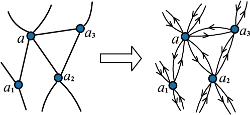
Figure 1: Any undirected edge in the network can be viewed as consisting of an outgoing edge and an incoming edge in the random walk models.

Instead of considering a single walker on a network, we assume $N$ ($N\gg 1$) mutually non-interacting classical walkers that move on a connected complex network with $M$ nodes. The move of walkers is ergodic and will reach an equilibrium after a substantial long period of time. It strongly suggests that we view the steady state as a thermal state in equilibrium. As shown in Fig.1, any undirected edge of the network can be viewed as consisting of two directed links. Each node in the network has equal numbers of outgoing and incoming links attached to it. In the steady state, the distribution of walkers $\{n_{a}\}$ does not change in time. This is only possible when all the directed links, outgoing and incoming, have the same flux of walkers at each time step. It is easily checked that the steady state has the walker distribution $\{n_{a}=NK_{a}/K\}$ or equivalently, the probability distribution $\{P_{a}=K_{a}/K\}$.

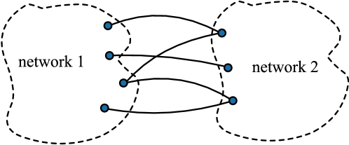
Figure 2: The network $1$ with $M_{1}$ nodes and total degree $K^{(1)}$ is linked to the network $2$ with $M_{2}$ nodes and total degree $K^{(2)}$. The number of linking edges $\ell$ between the network $1$ and $2$ is assumed to be small such that $\ell<<K^{(1)},K^{(2)}$ is satisfied. In the figure only the linked nodes between the two networks are shown.

In classical thermodynamics the concept of temperature is a property of a system that determines if thermal equilibrium exists with some other system. Once the steady state of random walks is viewed as a thermal equilibrium state then it is possible to define the “temperature” for the steady state. To find the temperature let’s consider the contact of two random walk systems, the network $1$ of $N_{1}$ walkers with $M_{1}$ nodes and the network $2$ of $N_{2}$ walkers with $M_{2}$ nodes. Both random walk systems are assumed to be in their steady states. So the number of walkers on node $a$ in the network $1$ is $n^{(1)}_{a}=N_{1}K^{(1)}_{a}/K^{(1)}$, where $K^{(1)}_{a}$ is the degree of node $a$ and $K^{(1)}$ is the total degree of the network $1$. Similarly, the number of walkers on node $b$ in the network $2$ is $n^{(2)}_{b}=N_{2}K^{(2)}_{b}/K^{(2)}$ with $K^{(2)}_{b}$ being the degree of node $b$ and $K^{(2)}$ being the total degree of the network $2$. We then bring the two systems together and join them by linking $\Delta M_{1}$ nodes of the network $1$ to $\Delta M_{2}$ nodes of the network $2$ as shown in Figure 2. The number of linking edges $\ell$ between the two networks is assumed to be much smaller than $K^{(1)}$ and $K^{(2)}$. Under the small $\ell$ assumption the total degree of the combined network can be thought of as the sum of the degrees of the two networks. The combined network now has $N=N_{1}+N_{2}$ walkers moving on it with $M=M_{1}+M_{2}$ nodes and the total degree $K=K^{(1)}+K^{(2)}$. When the distribution of walkers reaches an equilibrium in the combined system , the number of walkers $\tilde{n}^{(1)}_{a}$ on node $a$ in the network $1$ and the the number of walkers $\tilde{n}^{(2)}_{b}$ on node $b$ in the network $2$ are

$$\tilde{n}^{(1)}_{a}=\frac{N_{1}+N_{2}}{K^{(1)}+K^{(2)}}K^{(1)}_{a},$$ (3)

$$\tilde{n}^{(2)}_{b}=\frac{N_{1}+N_{2}}{K^{(1)}+K^{(2)}}K^{(2)}_{b}.$$ (4)

The differences $(\tilde{n}^{(1)}_{a}-n^{(1)}_{a})$ and $(\tilde{n}^{(2)}_{b}-n^{(2)}_{b})$ are thus found as

$$\tilde{n}^{(1)}_{a}-n^{(1)}_{a}=\frac{N_{1}N_{2}}{K^{(1)}K}(\frac{K^{(1)}}{N_{1}}-\frac{K^{(2)}}{N_{2}})K^{(1)}_{a},$$ (5)

$$\tilde{n}^{(2)}_{b}-n^{(2)}_{b}=\frac{N_{1}N_{2}}{K^{(2)}K}(\frac{K^{(2)}}{N_{2}}-\frac{K^{(1)}}{N_{1}})K^{(2)}_{b}.$$ (6)

From the results in Eq.s(5,6) the net flow of walkers will go from network $2$ to network $1$ if $K^{(1)}/N_{1}>K^{(2)}/N_{2}$ is satisfied. When $K^{(1)}/N_{1}<K^{(2)}/N_{2}$ the net flow of walkers will go from network $1$ to network $2$. There is no net flow of walkers between the two networks if the ratio $K^{(1)}/N_{1}$ equals $K^{(2)}/N_{2}$. It thus suggests that the ratio $K/N$ could be the candidate of “temperature” for the steady state of the random walk on a network of $N$ walkers with total degree $K$. It is interesting to note that, with the ratio $K/N$ being identified as the temperature for a random walk in equilibrium, the final temperature after combining two equilibrium random walks is always between the two temperatures of the two random walks before combining them. In the next section more reasons will be provided for identifying $K/N$ as the temperature.

III Canonical distribution for classical random walks on networks

The probability of obtaining the distribution of walkers $\{n_{a}\}$ over nodes is found as

$$P(\{n_{a}\};N,\{K_{a}\})=\frac{N!}{K^{N}}\prod_{a}\frac{K_{a}^{n_{a}}}{n_{a}!}.$$ (7)

The result in (7) is obtained by using the probability distribution $\{P_{a}=K_{a}/K\}$ for a single walker and then calculate the probability of having the walker distribution $\{n_{a}\}$. In the large $N$ limit, it has

$$\ln P(\{n_{a}\};N,\{K_{a}\})=-\frac{N}{K}\sum_{a}\xi_{a}\ln(\frac{\xi_{a}}{K_{a}})+O(\ln N).$$ (8)

Here $\xi_{a}\equiv n_{a}K/N$ ranges from $0$ to $K$. The steady state $|\pi\rangle$ corresponds to the distribution of $\xi_{a}$, $\{\xi_{a}=K_{a}\}$. From (8), we find the relative frequency $\Omega$ for the distribution $\{\xi_{a}\}$

$$\Omega(\{\xi_{a}\},\frac{K}{N},\{K_{a}\})=\exp[{-\frac{N}{K}H(\{\xi_{a}\};\{K_{a}\})}],$$ (9)

with

$$H(\{\xi_{a}\};\{K_{a}\})\equiv\sum_{a}\xi_{a}\ln(\frac{\xi_{a}}{K_{a}}).$$ (10)

The relative frequency $\Omega$ resembles the canonical distribution for a thermal system with Hamiltonian $H(\{\xi_{a}\};\{K_{a}\})$ that is in equilibrium with a heat bath at temperature $T=K/N$. The Hamiltonian $H(\{\xi_{a}\};\{K_{a}\})$ is easily proved to be non-negative and has the minimum $H_{min}=0$ which corresponds to the steady state, i.e., $\{\xi_{a}=K_{a}\}$. The temperature is identified as $T=K/N$ since when $\beta=1/T$ increases the expectation value of $\langle H\rangle$ will decrease and the system is likely to lie in the low-energy states.

III.1 Partition function, Helmholtz free energy, and the entropy

The partition function for the random walk system is calculated as follows. Consider the expansion of Hamiltonian $H(\{\xi_{a}\};\{K_{a}\})$

$$H(\{\xi_{a}\};\{K_{a}\})=\sum_{a=1}^{M}\frac{(\xi_{a}-K_{a})^{2}}{2K_{a}}+O(\Delta\xi^{3}).$$ (11)

Here $\Delta\xi$ and $(\xi_{a}-K_{a})$ are of the same order of magnitude. The partition function $Q_{M}$ for the thermal system is defined as

$$Q_{M}\equiv\sum_{\{\xi_{a}\}}\exp[-\beta H(\{\xi_{a}\};\{K_{a}\})].$$ (12)

Define new variables $\chi_{a}\equiv(\xi_{a}-K_{a})$ so that $\sum_{a}\chi_{a}=0$ is satisfied. We then calculate $Q_{M}$ and get

$$Q_{M} \simeq \int\{\prod_{a=1}^{M}d\chi_{a}\}\delta(\sum_{a}\chi_{a})\exp[-\sum_{a=1}^{M}\frac{\beta\chi_{a}^{2}}{2K_{a}}]$$ (13)

$$= (\frac{2\pi}{\beta})^{(M-1)/2}K^{-1/2}\prod_{a=1}^{M}K_{a}^{1/2}.$$

From the partition function $Q_{M}$ in (13), we find the average “energy” for the random walk system in equilibrium

$$\langle H\rangle=-\frac{\partial\ln Q_{M}}{\partial\beta}=\frac{(M-1)K}{2N}=\frac{(M-1)}{2}T.$$ (14)

The result in (14) is exactly the equipartition of energy in thermodynamics. The total degree of freedom for the random walk system is $(M-1)$ as can be easily seen from the number of independent variables in the Hamiltonian $H(\{\xi_{a}\};\{K_{a}\})$, and each degree of freedom acquires the same average energy $T/2$.

The Helmholtz free energy $F$ for the random walk system is found by

$$F\equiv\frac{-1}{\beta}\ln Q_{m}=-\frac{T}{2}\{(M-1)\ln(2\pi T)-\ln K+\sum_{a=1}^{M}\ln K_{a}\}.$$ (15)

From the Helmholtz free energy we obtain the entropy $S$ for the system

$$S\equiv-\frac{\partial F}{\partial T}=\frac{M-1}{2}[\ln(2\pi T)+1]-\frac{1}{2}\ln K+\frac{1}{2}\sum_{a=1}^{M}\ln K_{a}.$$ (16)

Obviously, the entropy $S$ in (16) does satisfy the relation $\partial S/\partial\langle H\rangle=1/T$. All state functions in the equations (14$\sim$16) depend (at least partially) on the state variables $M,T,K$, and $\{K_{a}\}$.

The entropy $S$ consists of two parts

$$S = -\frac{M-1}{2}\ln N+S_{top},$$ (17)

$$S_{top} = \frac{M-1}{2}\ln(2\pi e)+\frac{M-2}{2}\ln K+\frac{1}{2}\sum_{a=1}^{M}\ln K_{a},$$ (18)

where $S_{top}$ denotes the part solely determined by the topology of the complex network. In general, without changing the network topology the entropy $S$ decreases as the total number of walkers $N$ increases. On the other hand $S_{top}$ seems like to be an interesting property of the complex network. First, the topological entropy $S_{top}$ will increase by adding more edges to the network. For example, an edge is added to the network between node $a$ and node $b$. As a result, both the degree $K_{a}$ and $K_{b}$ are increased by $1$, the total degree $K$ is increased by $2$, and the topological entropy is changed by $\Delta S_{top}$

$$\Delta S_{top}=\frac{M-2}{2}\ln(1+\frac{2}{K})+\frac{1}{2}\{\ln(1+\frac{1}{K_{a}})+\ln(1+\frac{1}{K_{b}})\}>0.$$ (19)

Second, adding more nodes to the network also increases $S_{top}$. Suppose a new node is connected to nodes $1,2,\dots,q$ of the network. In the situation the number of nodes is increased by $1$, all the degrees of nodes $1,2,\dots,q$ are increased by $1$, and the total degree is increased by $2q$. Thus the change in $S_{top}$ is

$$\Delta S_{top} = \frac{M-1}{2}\ln(1+\frac{2q}{K})+\frac{1}{2}[\ln(2\pi K)+1]+\frac{1}{2}\sum_{a=1}^{q}\ln(1+\frac{1}{K_{a}})+\frac{1}{2}\ln q$$ (20)

$$> 0.$$

From the results in (19) and (20) we conclude that the topological entropy $S_{top}$ always increases as more nodes or edges are added to complex networks. It strongly suggests that the topological entropy $S_{top}$ could be used as a measure of network complexity. Among all connected networks with $M$ nodes, the star topology (e.g. the network A in Fig.3 for $M=5$) has the minimum value of $S_{top}$

$$S^{(min)}_{top}(M)=\frac{M-1}{2}\{\ln[2\pi(M-1)]+1\}+\frac{M-2}{2}\ln 2,$$ (21)

while the fully connected topology (e.g. the network L in Fig.3 for $M=5$) has the maximum value of $S_{top}$

$$S^{(max)}_{top}(M)=\frac{M-1}{2}\{\ln[2\pi(M-1)^{2}]+1\}+\frac{M-2}{2}\ln M.$$ (22)

As an example, let’s consider four networks A, F, K and L as shown in Figure 3. All the four networks have five nodes but are of different topologies. Among the four networks the star topology (network A) has the minimum value of $S_{top}$ while the fully connected topology (network L) has the maximum $S_{top}$. All nodes in the network A have just one edge linked to them except for a central node that is connected to all other nodes. Contrarily, the network L has no central node. Any two nodes are linked by an edge in the network L. It has $S^{L}_{top}=13.635>S^{K}_{top}=12.725>S^{F}_{top}=10.863>S^{A}_{top}=9.488$. The above result suggests that the network A is less complex than the network F, the network F is less complex than the network K, and the network K is less complex than the network L.

IV Random walk with a probability of resting on nodes

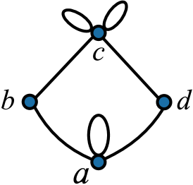
Figure 4: A network with self-linked edges. Node $a$ has one self-linked edge and node $c$ has two self-linked edges.

In the section we consider a slightly different scenario: a walker has a prior probability $\sigma_{a}$ of resting on node $a$ at each time step. The scenario is indeed related to the random walks on the connected networks that have self-linked edges linking a node to itself. As an example let’s consider a connected network with self-linked edges as shown in Figure 4. A self-linked edge is attached to node $a$ and two self-linked edges are attached to node $c$. Since each self-linked edge contributes the amount of $2$ to the degree, we thus find the degrees of the nodes to be $\{K_{a}=4,K_{b}=2,K_{c}=6,K_{d}=2\}$ and the total degree of the network is $K=14$. For a walker on node $c$ at time step $t$, it has the probability $1/6$ of hopping to node $b$ or $d$ at the next time step. In other words, it has the probability $2/3$ of resting on node $c$ at time step $t+1$. Similarly, a walker on node $a$ at time step $t$ could stay on the same node with the probability $2/4$ at the next time step. From the distribution of degrees we thus find the probabilities of finding a walker on the nodes in the steady state, $\{P_{a}=4/14,P_{b}=2/14,P_{c}=6/14,P_{d}=2/14\}$.

The discussion is easily generalized to the case of $N$ non-interacting random walkers moving on a connected network of $M$ nodes with the degree distribution $\{K_{a}\}$ and the distribution of prior resting probability on nodes $\{\sigma_{a}\}$. Once again, here $\sigma_{a}$ denotes the probability of resting on node $a$ at the next time step for a single walker. The case is equivalent to a conventional random walk on a network of $M$ nodes with the degree distribution $\{K_{a}^{\prime}\}$,

$$K_{a}^{\prime} = K_{a}+2L_{a}=\frac{K_{a}}{(1-\sigma_{a})},$$ (23)

$$L_{a} = \frac{\sigma_{a}}{2(1-\sigma_{a})}K_{a},$$ (24)

where $L_{a}$ denotes the number of the self-linked edges attached to node $a$. In general, $L_{a}$ ranges from zero to infinity and may not be an integer. We thus find the temperature $T$ of the modified random walk model as

$$T=\frac{K^{\prime}}{N},$$ (25)

with the effective total degree $K^{\prime}$

$$K^{\prime}=\sum_{a}\frac{K_{a}}{(1-\sigma_{a})}.$$ (26)

The probability of having the walker distribution $\{n_{a}\}$ is thus found by

$$P(\{n_{a}\};N,\{K_{a}\},\{\sigma_{a}\})=\frac{N!}{K^{\prime N}}\prod_{a}\frac{1}{n_{a}!}[\frac{K_{a}}{(1-\sigma_{a})}]^{n_{a}}.$$ (27)

The probability distribution $P(\{n_{a}\};N,\{K_{a}\},\{\sigma_{a}\})$ depends not only on the topology of the network but also on the distribution of the node-resting probability $\{\sigma_{a}\}$. In fact, it is better to view $\{\sigma_{a}\}$ as one of the topological factors of the network. Other state functions such as the average energy, the Helmholtz free energy, and the entropy of the modified random walk system are obtained by replacing $K_{a}$ with $K_{a}^{\prime}$, and replacing $K$ with $K^{\prime}$ in the equations (14, 15, 16). For example, the topological part of the entropy in the modified random walk model is

$$S_{top}=\frac{M-1}{2}\ln(2\pi e)+\frac{M-2}{2}\ln K^{\prime}+\frac{1}{2}\sum_{a=1}^{M}\ln K_{a}^{\prime}.$$ (28)

In conclusion, the effect of resting on nodes is equivalent to increasing the degree at every node in the network. The topological entropy also increases in the modified random walk as compared to that in the conventional random walks without the prior resting probability.

V Discussion

In this paper we consider $N$ non-interacting classical walkers that move on a connected network with $M$ nodes and the distribution of degrees $\{K_{a}\}$. We found that the steady state of the random walk system can be interpreted as a thermal state in equilibrium. We then identified the temperature for the system to be $K/N$, where $K$ is the total degree, and calculated various state functions of the system such as the average energy $\langle H\rangle$, the Helmholtz free energy, and the entropy $S$. The results show that the equilibrium thermal state has the property of equipartition of energy. Without changing the network topology the entropy $S$ increases as the total number of walkers decreases. In fact, the entropy $S$ consists of two parts. The first part depends solely on the number of walkers $N$ and the number of nodes $M$. The second part, called the topological entropy $S_{top}$ in the paper, depends solely on the network topology. In general, $S_{top}$ will increase as more edges or nodes are added to the network. It thus suggests that $S_{top}$ can be used as a measure of network complexity.

There is no absolute definition of what complexity of networks means. Even without a precise definition of network complexity, a few descriptors are used as measures of network structure (complexity, ; descriptors, ). For example, the information theoretic index for node degree distribution

$$I_{vc}\equiv K\log_{2}K-\sum_{a=1}^{M}K_{a}\log_{2}K_{a},$$ (29)

which makes use of Shannon’s formula for the total information content of the vertex distribution. Usually $I_{vc}$ increases with the connectivity and other complexity factor such as the number of cycles. As shown in Fig. 3, the total degree $K$ increases from $K=8$ to $K=20$ for the five-node graphs from A to L. The plot of the normalized index

$$\tilde{I}_{vc}=\frac{I_{vc}}{I^{(max)}_{vc}},$$ (30)

is shown in Fig. 5 with $I^{(max)}_{vc}$ being the maximum of $I_{vc}$ for the five-node networks. It shows that $I_{vc}$ does increase with connectivity. The number of cycles is also considered as a stronger network complexity factor, and this is seen in the sequence of graphs with one to five cycles: F $\rightarrow$ H $\rightarrow$ J $\rightarrow$ K $\rightarrow$ L. Another useful descriptor that describes the overall degree of network clustering is the average clustering coefficient $\langle C\rangle$

$$\langle C\rangle = \frac{\sum_{a}C_{a}}{M},$$ (31)

$$C_{a} = \frac{2f_{a}}{K_{a}(K_{a}-1)}.$$ (32)

Here $f_{a}$ denotes the number of edges that link the first neighbors of node $a$, and $C_{a}$ is the clustering coefficient of node $a$. As seen in Fig. 3, the clustering coefficients of all nodes in the acyclic graphs A, B, and C, are zero. All vertices in cyclic graphs having four or more vertices also have zero clustering coefficients. Nonzero clustering coefficients can only be obtained in tri-membered cycles. More tri-membered cycles in a graph usually give a higher $\langle C\rangle$ value, as can be seen in the sequence of graphs with one to three tri-membered cycles: D $\rightarrow$ G $\rightarrow$ J. Other descriptors such as the $B2$ and $B3$ indices make use of vertex and vertex distance distribution

$$B2 = \sum_{a=1}^{M}\frac{K_{a}}{D_{a}},$$ (33)

$$B3 = B2\log_{2}B2-\sum_{a=1}^{M}\frac{K_{a}}{D_{a}}\log_{2}\frac{K_{a}}{D_{a}}.$$ (34)

Here $D_{a}$ is the sum of all the minimum distances $D_{ab}$ between node $a$ and other nodes (node $b$)

$$D_{a}=\sum_{b\neq a}D_{ab}.$$ (35)

The indices $B2$ and $B3$ increase with the connectivity and the number of cycles, similar to the index $I_{vc}$. However, unlike the index $I_{vc}$, $B2$ also increases with the appearance of an additional branch. This is seen in the plot of the normalized $B2$ index in Fig. 5 for the sequences of graphs of the same total degree: C $\rightarrow$ B $\rightarrow$ A, F $\rightarrow$ E $\rightarrow$ D, H $\rightarrow$ G, J $\rightarrow$ I.

In order to compare the topological entropy $S_{top}$ and the other network descriptors $I_{vc},\langle C\rangle$ and $B2$, the descriptors are normalized and thus range from $0$ to $1$. For example, the graph L in Fig. 3 has the maximum value of $I_{vc}=46.439$ among all the five-vertex graphs. We thus define the normalized index $\tilde{I}_{vc}=I_{vc}/46.439$. Similarly, the normalized $B2$ index is defined as $\tilde{B}_{2}=B_{2}/5.0$ for all the five-vertex graphs in Fig. 3. The normalized topological entropy $\tilde{S}_{top}$ for all $M$-node networks is defined as

$$\tilde{S}_{top}=\frac{S_{top}-\frac{M-1}{2}\ln(2\pi e)}{\{S_{top}-\frac{M-1}{2}\ln(2\pi e)\}_{max}}.$$ (36)

The term $(M-1)\ln(2\pi e)/2$ is subtracted from $S_{top}$ in equation (36) since it is the same for all $M$-node connected networks. A plot of $\tilde{S}_{top}$, $\tilde{I}_{vc}$, $\langle C\rangle$, and $\tilde{B}_{2}$ for all the five-node networks in Fig. 3 is given in Fig. 5. As easily seen from Fig. 5, $\tilde{S}_{top}$ and $\tilde{I}_{vc}$ behave similarly as descriptors of network structure. Both of them increase with the connectivity and the number of cycles. Contrary to the $\tilde{B}2$ index, $\tilde{S}_{top}$ will decrease with the appearance of an additional branch. Thus the network with star topology will have the minimum value of $S_{top}$, while the network of a chain of nodes will have the minimum value of $B2$. All the descriptors in Fig. 5 will reach their maximum values when the network has a fully connected topology.

Although $S_{top}$ behaves like $I_{vc}$ for the five-vertex networks in Fig. 3, they are different in a few aspects. First, the topological entropy $S_{top}$ depends explicitly on the total number of $M$ while $I_{vc}$ depends on $M$ implicitly. This originates from the fact that the index $I_{vc}$ makes use of Shannon’s formula for the total information content of the vertex distribution, while the topological entropy $S_{top}$ makes use of the distribution of classical random walkers over nodes. Second, the order of magnitude of $S_{top}$ for any $M$-vertex networks is $O(M\log M)$. On the other hand, the order of magnitude of $I_{vc}$ is $O(M\log M)$ for the network of a star-like topology, and is $O(M^{2}\log M)$ for the network of a fully connected topology. It means that $I_{vc}$ increases much more rapidly than $S_{top}$ when more and more edges are appearing between nodes. This is shown in Fig. 6 for 100-vertex networks. For any networks with fixed number of nodes $M$ and fixed total degree $K$, the indices $I_{vc}(M,K;\{K_{a}\})$ and $S_{top}(M,K;\{K_{a}\})$ descriptors are viewed as functions of the node distribution $\{K_{a}\}$. Theoretically, there are upper bounds for $I_{vc}(M,K;\{K_{a}\})$ and $S_{top}(M,K;\{K_{a}\})$ with fixed values of $M$ and $K$

$$I_{vc}(M,K;\{K_{a}\}) \leq I_{vc}(M,K;\{K_{a}=K/M\})=K\log_{2}M,$$ (37)

$$S_{top}(M,K;\{K_{a}\}) \leq S_{top}(M,K;\{K_{a}=K/M\})$$ (38)

$$= \frac{M-1}{2}[\ln(2\pi)+1]-\frac{M}{2}\ln M+(M-1)\ln K.$$

The results in the above equations show that the upper bound of $I_{vc}$ increases linearly with $K$ for $M$-node networks, and the upper bound of $S_{top}$ is a linear function of $\log K$ for $M$-node networks. After truncating the $K$-independent terms in (38), the truncated upper bound of $S_{top}$ is normalized as

$$S^{\prime}_{top}=\frac{\ln K}{\ln(M(M-1))}.$$ (39)

The normalized upper bound $I^{\prime}_{vc}$ is defined as

$$I^{\prime}_{vc}=\frac{K}{M(M-1)}.$$ (40)

Fig. 6 shows the normalized upper bounds $I^{\prime}_{vc}$ and $S^{\prime}_{top}$ for $M=100$. The total degree $K$ ranges from $2(M-1)$ to $M(M-1)$ in Eq.(40) and (39). When $M$ is large, $S^{\prime}_{top}$ goes approximately from $0.5$ to $1.0$ as $K$ increases, different to the upper bound $I^{\prime}_{vc}$ that goes approximately from zero to $1.0$. For most of the values of $K$, $S^{\prime}_{top}$ is a slow-changing function of $K$ as compared to $I^{\prime}_{vc}$.

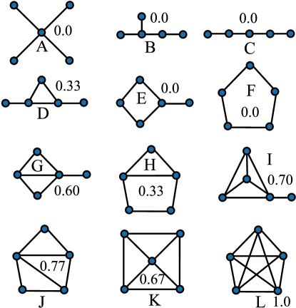
Figure 3: The topological entropies for the five-node networks are $S^{A}_{top}=9.488$, $S^{B}_{top}=9.691$, $S^{C}_{top}=9.835$, $S^{D}_{top}=10.575$, $S^{E}_{top}=10.719$, $S^{F}_{top}=10.863$, $S^{G}_{top}=11.339$, $S^{H}_{top}=11.541$, $S^{I}_{top}=11.975$, $S^{J}_{top}=12.119$, $S^{K}_{top}=12.725$, and $S^{L}_{top}=13.635$. The numbers in the figure denote the average clustering coefficient $\langle C\rangle$ for each network.

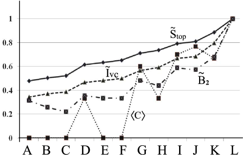
Figure 5: Plots of network descriptors $\tilde{S}_{top}$, $\tilde{I}_{vc}$, $\tilde{B}2$, and $\langle C\rangle$ for the five-vertex graphs listed in Fig. 3. The descriptors $\tilde{S}_{top}$, $\tilde{I}_{vc}$, and $\tilde{B}2$ are the normalized indices of $S_{top}$, $I_{vc}$, and $B2$.

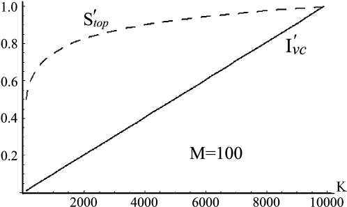
Figure 6: The normalized upper bounds $S^{\prime}_{top}$ (truncated) and $I^{\prime}_{vc}$ for 100-vertex networks as functions of the total degree $K$.

- (1) N. Ganguly, A. Deutsch and A. Mukherjee (Eds), Dynamics on and of Complex Networks: Applications to Biology, Computer Science, and the Social Sciences (Birkhäuser Science, 2009); G. Caldarelli and M. Catanzaro, Networks: A Very Short Introduction (Oxford University Press, 2012); E. Estrada, The Structure of Complex Networks: Theory and Applications (Oxford University Press, 2011).
- (2) J. F. F. Mendes and S. N. Dorogovtsev, Evolution of Networks: From Biological Nets to the Internet and WWW (Oxford Press, New York, 2003).
- (3) A.-L. Barabási and Z. N. Oltvai, Nat. Rev. Genet. 5, 101 (2004).
- (4) B. M. Leiner, V. G. Cerf, D. D. Clark, R. E. Kahn, L. Kleinrock, D. C. Lynch, J. Postel, L. G. Roberts and S. Wolff, “Brief History of the Internet”, Internet Society (2012); W. Willinger, D. Alderson, and J. C. Doyle, Notices of the AMS 56, 586-599 (2009); R. Pastor-Satorras and A. Vespignani, Evolution and Structure of the Internet: A Statistical Physics Approach (Cambridge University Press, Cambridge, U.K., 2004).
- (5) E. F. Churchill and C. A. Halverson, “Social Networks and Social Networking”, IEEE Internet Computing, September/October(2005);
- (6) P. Erdös and A. Rényi, Publ. Math., Debrecen 6, 290-297 (1959).
- (7) P. Erdös and A. Rényi, Publ. Math. Inst. Hung. Acad. Sci. Ser. A 5, 17-61 (1960).
- (8) R. Albert, H. Jeong and A.Barabási, Nature 401, 130-131 (1999).
- (9) D. J. Watts and S. H. Strogatz, Nature 393, 440-442 (1998).
- (10) S. Zhou and R. J. Mondragón, IEEE commun. Lett., vol. 8, 180-182 (2004).
- (11) A.-L. Barabási and R. Albert, Science 286, 509 (1999).
- (12) R. Albert, A.-L. Barabási,, and H. Jeong, Physica A 272, 173 (1999).
- (13) K. Takemoto and C. Oosawa, Phys. Rev. E 72, 046116(2005).
- (14) R. Albert and A.-L. Barabási, Rev. Mod. Phys. 74, 47 (2002).
- (15) R. D. Hughes, Random Walks: Random Walks and Random Environments (Clarendon, Oxford, 1995),Vol. 1.
- (16) J. R. Norris, Markov chains (Cambridge University Press, 1998).
- (17) L. Mlodinow, The Drunkard’s Walk: How Randomness Rules Our Lives (Pantheon Books, 2008).
- (18) J. D. Noh and H. Rieger, Phys. Rev. Lett. 92, 118701 (2004).
- (19) J. Keizer, Journal of Statistical Physics 6, 67-72 (1972); P. Lancaster and M. Tismenetsky, Theory of matrices, Vol. 2 (Academic Press New York, 1985).
- (20) A. H. Carter, Classical and Statistical Thermodynamics (Prentice-Hall, 2001).
- (21) D. Bonchev and G. A. Buck, “Quantitative Measures of Network Complexity”, in Complexity in Chemistry, Biology, and Ecology (Springer, 2005), 191-236.
- (22) D. Bonchev and G. A. Buck, J. Chem. Inf. Model. 47, 909-917 (2007).