Non-relativistic high-energy physics: top production and dark matter annihilation

Abstract

Non-relativistic physics is often associated with atomic physics and low-energy phenomena of the strong interactions between nuclei and quarks. In this review we cover three topics in contemporary high-energy physics at or close to the TeV scale, where non-relativistic dynamics plays an important if not defining role. We first discuss in detail the third-order corrections to top-quark pair production in electron-positron collisions in the threshold region, which plays a major role at a future high-energy $e^{+}e^{-}$ collider. Threshold effects are also relevant in the production of heavy particles in hadronic collisions, where in addition to the Coulomb force soft gluon radiation contributes to enhanced quantum corrections. We review the joint resummation of non-relativistic and soft gluon effects for pair production of top quarks and supersymmetric particles to next-to-next-to-leading logarithmic accuracy. The third topic deals with pair annihilation of dark matter particles within the framework of the Minimal Supersymmetric Standard Model. Here the electroweak Yukawa force generated by the exchange of gauge and Higgs bosons can cause large “Sommerfeld” enhancements of the annihilation cross section in some parameter regions.

1 Introduction

Non-relativistic particle physics is often associated with atomic physics, the interactions between nuclei, and the low-energy phenomena of the strong interactions of the charm and bottom quarks, which form quarkonium bound states. But non-relativistic dynamics also governs the interactions of weak-scale particles such as the top quark or the hypothetical supersymmetric partners of the Standard Model (SM) particles, when they are slowly moving. In this review we cover three topics in contemporary high-energy physics where the unique non-relativistic dynamics caused by instantaneous, potential interactions plays an important if not defining role: the production of top-quark pairs in electron-positron collisions in the threshold region, which can provide a measurement of the top-quark mass with unchallenged precision and could be realized at a future high-energy $e^{+}e^{-}$ collider. The hadronic pair production of top quarks at Tevatron and LHC, or yet unobserved heavy particles at the LHC, where in addition to the Coulomb force soft gluon radiation contributes to enhanced quantum corrections, which should be summed. And finally, the pair annihilation of dark matter particles within the framework of the Minimal Supersymmetric Standard Model (MSSM). While the first two processes are determined by the long-range colour Coulomb force, the low-velocity annihilation of heavy neutralinos in the MSSM can be dramatically enhanced by the short-range electroweak Yukawa force generated by the exchange of gauge and Higgs bosons.

We discuss the phenomena and results but also emphasize theoretical methods and techniques. Since there is always a small relative velocity $v$ in the problem, non-relativistic systems involve (at least) the three scales $m$ (mass), $mv$ (momentum), $mv^{2}$ (energy), and it is appropriate to formulate effective Lagrangians to organize the calculation, even if the underlying theory — QCD, the SM, or the MSSM — is known. The three topics discussed here have further in common that the relevant Lagrangian couplings are weak at all three scales. This allows for a systematic treatment with approximations of well-defined parametric accuracy, even though ordinary perturbation theory in the coupling breaks down, as will be discussed.

Each of the three topics provides its own specific challenges. In top-quark pair production near threshold in $e^{+}e^{-}$ collisions, it is the high precision of the envisioned mass measurement, which demands calculations with unprecedented third-order accuracy in the non-relativistic approximation that can be achieved by a combination of effective field theory and multi-loop techniques. In hadronic production the required precision is less, but the coloured partonic initial state of quarks and gluons implies that soft-gluon resummation must be integrated into the non-relativistic expansion, and a more general treatment of colour is needed for final states which can be produced in various colour representations. Dark matter (DM) annihilation involves yet another issue. The non-relativistic “Sommerfeld” enhancements from electroweak gauge boson exchange are operative only, when the DM particles are in the TeV range, such that the inverse Bohr radius scale is of order of or larger than the mass of the electroweak gauge bosons. For such heavy, weakly interacting particles, the mass splitting between the members of the electroweak multiplet are small, so that co-annihilation effects at dark matter freeze-out are generic. While the non-relativistic treatment is only performed at leading-order, the complexity of the problem arises from a large number of interacting two-particle states, kinematically closed channels in the Schrödinger problem, which must be solved numerically, and the large number of final states that contribute to the pair annihilation cross section in a model such as the MSSM.

The outline of this review is as follows: in the next section we briefly summarize several methods and technical tools, which are necessary to perform the calculations. In particular, we briefly describe the threshold expansion, introduce NRQCD and PNRQCD, and mention a few details in connection to the underlying multi-loop calculations. Section 3 is devoted to the top-quark pair production cross section near threshold in $e^{+}e^{-}$ annihilation. We introduce the main ingredients in the third-order calculation and discuss the numerical results. In Section 4 top-quark and supersymmetric pair production is considered at hadron colliders. After describing the joint soft and Coulomb resummation formalism, the top-pair invariant mass distribution near threshold is considered. We then summarize results on the resummed total top and SUSY pair production cross sections, and compare it to fixed-order results, and results with soft-gluon but without Coulomb resummation. Section 5 leads through the effective field theory treatment of Sommerfeld enhancement in dark matter annihilation with a short discussion of a method to determine the enhancement reliably in situations with several channels without extreme degeneracies. We also highlight a few results for a wino-like dark matter particle and a series of models that interpolates from a Higgsino- to wino-like neutralino. We conclude our review with a summary in Section 6.

2 Methods and techniques

Before addressing more specifically the three topics of this review, we summarize the main methods and techniques.

2.1 Threshold expansion

Close to the production threshold of two heavy particles (for simplicity, with equal masses) there are three characteristic scales: the mass of the particle, $m$, its three-momentum of order $mv$, and the kinetic energy $\sqrt{s}-2m=mv^{2}$. For example, for top quarks we have $m\approx 170$ GeV, $mv\approx 20$ GeV and $mv^{2}\approx 2$ GeV, and thus a strong hierarchy among the scales. Furthermore, $mv^{2}\gg\Lambda_{\rm QCD}$, which means that the strong coupling $\alpha_{s}(\mu)$ is always in the perturbative regime. In this review, we only consider systems where this condition is satisfied.

The presence of the small parameter $v$ leads to a breakdown of the standard perturbation expansion in $\alpha_{s}$ due to kinematic $1/v$ enhancements. A reorganized, non-relativistic expansion must be used, where both $\alpha_{s}$ and $v$ are simultaneously considered as small but $\alpha_{s}/v$ of order one. In terms of Feynman diagrams, a summation of certain terms to all orders in $\alpha_{s}$ is required. At the same time, since $v$ is small, one does not need the full dependence on $v$ of every fixed-order diagram.

For a given Feynman diagram the expansion in $v$ can be constructed without first computing the full expression using the threshold expansion [1]. The method exploits that every diagram can be decomposed into a sum of terms, for which each loop momentum is in one of the following four momentum regions:

$$\mbox{hard (h)}: \ell^{0}\sim m, \mbox{\boldmath$\ell$\unboldmath}\sim m$$

$$\mbox{soft (s)}: \ell^{0}\sim mv, \mbox{\boldmath$\ell$\unboldmath}\sim mv$$

$$\mbox{potential (p)}: \,\ell^{0}\sim mv^{2}, \mbox{\boldmath$\ell$\unboldmath}\sim mv$$

$$\mbox{ultrasoft (us)}: \,\ell^{0}\sim mv^{2}, \mbox{\boldmath$\ell$\unboldmath}\sim mv^{2}\,\,$$ (1)

In each region the integrand of the Feynman diagram is expanded in the small parameters of the respective region. Afterwards the loop integration over the complete $d$-dimensional space-time volume is performed. The property of dimensional regularization that scaleless integrals vanish, guarantees that no double counting occurs. The arguments in favour of this construction provided in [1] rely on assumptions on the location of singularities in the Feynman integrand and examples. Further justification can be found in [2]. It may happen that the separation of the integrand into regions generates spurious ultraviolet and infrared divergences. However, they cancel in the sum of all contributions.

2.2 Non-relativistic effective theory

The procedure described in the previous subsection is essentially equivalent to the explicit construction of effective non-relativistic Lagrangians within dimensional regularization, since the terms that arise in the threshold expansion can be interpreted as modified propagators and vertices. In a certain sense, the threshold expansion defines these Lagrangians in dimensional regularization by providing the precise rules for performing consistent matching calculations.

To be definite, we refer to a system of a heavy quark (Q) and antiquark interacting via gluons. The effective Lagrangians are constructed in two steps following the following scheme for integrating out momentum modes:

$$\begin{array}[]{cc}{\cal L}_{\rm QCD}\,[Q(h,s,p),\,g(h,s,p,us)]&\mu>m\\[8.5359pt] \Big{\downarrow}&\\[8.5359pt] {\cal L}_{\rm NRQCD}\,[Q(s,p),\,g(s,p,us)]&mv<\mu<m\\[8.5359pt] \Big{\downarrow}&\\[8.5359pt] {\cal L}_{\rm PNRQCD}\,[Q(p),\,g(us)]&\mu<mv\\[8.5359pt] \end{array}$$

In square brackets the modes of the heavy quarks ($Q$) and massless particles ($g$) are displayed which are still contained in the effective Lagrangian; the others are integrated out when the energy scale $\mu$ is lowered as indicated on the right.

The first step leads to NRQCD [3, 4, 5]. Its Lagrangian has the following structure

$${\cal L}_{\rm NRQCD} = {\cal L}_{\psi}+{\cal L}_{\chi}+{\cal L}_{\psi\chi}+{\cal L}_{g}+{\cal L}_{\rm light}\,,$$ (2)

where explicit expressions of the individual contributions can be found in [6]. The bilinear heavy-quark Lagrangians ${\cal L}_{\psi}$ and ${\cal L}_{\chi}$ contain the kinetic terms for the two-component quark and antiquark fields $\psi$ and $\chi$ and the interactions with the chromomagnetic field in an expansion up to including terms of order $1/m^{3}$. ${\cal L}_{\psi\chi}$ contains four-fermion quark-antiquark terms and ${\cal L}_{g}$ is the pure gluon part, again expanded in $1/m$. Finally, ${\cal L}_{\rm light}$ is the same as the light-quark Lagrangian in full QCD. The Feynman rules derived from the Lagrangian (2) can, e.g., be found in [6]. All matching coefficients relevant for a third-order calculation can also be found in [6]. A subtlety that is explained there in detail is that the short-distance coefficient functions of the operators in the NRQCD Lagrangian must be kept $d$-dimensional in dimensional regularization.

In the second matching step in the above scheme soft modes and potential massless modes are integrated out. It has been suggested in the context of the threshold expansion in [1] and at the level of an effective Lagrangian in [7]. The result is the so-called potential NRQCD (PNRQCD) Lagrangian developed in various forms in [7, 8, 9, 10, 11]. It only contains ultrasoft light fields and potential heavy quarks, which simplifies the scaling in the velocity expansion. Note that since the components of the hard momentum integrated out in the first matching step are larger than those of the modes in the effective theory, the NRQCD Lagrangian is local. This can no longer be expected for PNRQCD. However, since only the three-momentum of the potential modes $Q(p)$ is of order of the soft scale $mv$, the non-locality of the PNRQCD Lagrangian refers only to space but not to time. The relevant terms in the PNRQCD Lagrangian are given by [6]

where

$$V_{ab;cd}(r,{\mbox{\boldmath${\partial}$}})=T^{A}_{ab}T^{A}_{cd}V_{0}(r)+\delta V_{ab;cd}(r,{\mbox{\boldmath${\partial}$}})\,.$$ (4)

$V_{0}=-\alpha_{s}/r$ is the tree-level colour Coulomb potential. The first two terms of ${\cal L}_{\rm PNRQCD}$ contain the kinetic terms including the relativistic corrections and the third term is responsible for heavy-quark potential interactions. Note that the heavy-quark potentials generated in the matching to PNRQCD enter this term as short-distance coefficients of the spatially non-local but temporally local, i.e. instantaneous, PNRQCD interactions. Ultrasoft interactions between the heavy quarks and the gluon field are contained in the last two terms of (LABEL:eq:pnrqcd) and the $A_{0}$ terms in the first line. The latter do not contribute to colour-singlet production of a $Q\bar{Q}$ pair, in which case ultrasoft effects enter for the first time at third order in non-relativistic perturbation theory.

Perturbation theory in PNRQCD closely resembles quantum-mechanical perturbation theory, since the leading colour-Coulomb interaction is part of the unperturbed theory. Thus, the propagator of PNRQCD includes the leading Coulomb interaction exactly, which effects the required resummation of conventional perturbation theory to all orders. The PNRQCD Feynman rules can again be found in [6].

2.3 Multi-loop calculations

The computation of matching coefficients with high precision involves fixed-order multi-loop calculations. For the topics reviewed in this article, the highest order is demanded in the calculation of the three-loop corrections to the static potential and the matching coefficient between QCD and NRQCD of the vector current. For calculations of this type it is necessary to have a high level of automation, which reaches from the generation of the Feynman diagrams to the final summation and expansion in $\epsilon$. The scheme used for the three-loop vector-current matching coefficient requires particularly little manual interaction and is described in detail in [12].

For the generation of the contributing Feynman diagrams we use the Fortran program QGRAF [13]. The output is passed via q2e [14, 15], which transforms Feynman diagrams into Feynman amplitudes, to exp [14, 15] that generates FORM [16, 17] code. At the same time a topology is assigned to each diagram. The FORM code is processed to perform traces, apply projectors, and map the resulting scalar expressions to functions, which have a one-to-one relation to the topologies. They contain the exponents of the involved propagators as arguments. At this point one has in general a large number of different functions. Thus, in a next step one passes them to a program which implements the Laporta algorithm [18] and performs a reduction to a small number of so-called master integrals. The latter have to be computed using analytical or numerical methods. In the case of the three-loop corrections to the static potential all but three coefficients in the $\epsilon$ expansion could be computed analytically. For the three-loop corrections to the matching coefficient a significant number of integrals have been evaluated numerically using the program FIESTA [19, 20, 21], which is based on sector decomposition.

3 Top-quark pair production near threshold in $e^{+}e^{-}$ annihilation

Top-quark pair production near threshold in $e^{+}e^{-}$ annihilation provides a unique possibility to measure a number of parameters with high precision. Among them are the top-quark mass and width, the strong coupling constant, and the top-quark Yukawa coupling. In particular the mass determination attracts lot of attention, since the current uncertainty can be improved by about an order of magnitude, and at the same time the renormalization scheme is precisely defined. To reach this goal precise predictions are needed including both QCD and electroweak higher order corrections. The top-antitop system near threshold involves only scales in the perturbative regime [22], which allows for systematic approximations. Next-to-next-to-leading order (NNLO) QCD corrections have been computed at the end of the 1990s by several independent groups [23, 24, 25, 26, 27, 28, 11]. The results are summarized and compared in [29]. The inclusion of the NNLO corrections led to a significant shift of the cross section, and the theoretical uncertainty estimated through scale dependence remained larger than naively expected. The prospect of an accurate mass measurement at a future high-energy $e^{+}e^{-}$ collider therefore makes it mandatory to push the theoretical calculation to the third order.

In this section we sketch the computation of the cross section $\sigma(e^{+}e^{-}\to t\bar{t}+X)$ close to threshold to third order in non-relativistic perturbation theory. Normalized to the cross section for the production of $\mu^{+}\mu^{-}$ pairs in the high-energy limit, $\sigma_{0}=4\pi\alpha^{2}/(3s)$, it is given by

$$R = \frac{\sigma(e^{+}e^{-}\to t\bar{t}+X)}{\sigma_{0}}$$ (5)

$$= 12\pi e_{t}^{2}\,\,\mbox{Im}\left[\Pi^{(v)}(q^{2}=s+i\epsilon)\right]\,,$$

where $e_{t}=2/3$ is the top-quark electric charge, and the vector polarization function near threshold has the form

$$\Pi^{(v)}(q^{2}) = \frac{N_{c}}{2m_{t}^{2}}\,c_{v}\left[c_{v}-\frac{E}{m_{t}}\,\left(c_{v}+\frac{d_{v}}{3}\right)\right]$$ (6)

$$\mbox{}\times G(E)+\ldots\,.$$

For simplicity of notation, we restrict this expression to the terms from a virtual photon, neglecting the $Z$-boson contribution. The full expressions are given in [6]. $c_{v}$ and $d_{v}$ are NRQCD matching coefficients with perturbative expansions in $\alpha_{s}$, which are defined through the expansion of the vector current $j^{(v)\,\mu}$ in terms of non-relativistic fields given by

$$j^{(v)\,i}=c_{v}\,\psi^{\dagger}\sigma^{i}\chi+\frac{d_{v}}{6m_{t}^{2}}\,\psi^{\dagger}\sigma^{i}\,{\bf D^{2}}\chi+\ldots.$$ (7)

The terms proportional to $E=\sqrt{s}-2m_{t}$ in (6) arise from expanding the prefactor $1/q^{2}=1/s$ and from the $1/m_{t}^{2}$ suppressed current in (7), whose matrix element can be reduced to the one of the leading current by equation-of-motion relations. Thus, the central quantity in the non-relativistic representation is the two-point function

$$G(E)=\frac{i}{2N_{c}(d-1)}\int d^{d}x\,e^{iEx^{0}}\,$$ (8)

$$\mbox{}\langle 0|\,T(\,[\chi^{{\dagger}}\sigma^{i}\psi](x)\,[\psi^{{\dagger}}\sigma^{i}\chi](0))|0\rangle_{|\rm NRQCD}$$

of non-relativistic currents, which has to be computed within NRQCD.

In the following subsections we discuss various ingredients which are needed for the third-order prediction to $\sigma(e^{+}e^{-}\to t\bar{t}+X)$. In particular, we describe in Section 3.1 the calculation of the three-loop corrections to the matching coefficient $c_{v}$ and in Section 3.2 the three-loop corrections to the static potential. The latter is an important ingredient for the non-relativistic correlator which is discussed in Section 3.3. Ultrasoft corrections appear for the first time at third order and are discussed in Section 3.4 before presenting results for S-wave QCD contribution to the third-order cross section in Section 3.5. Section 3.6 contains further results, in particular a discussion of Higgs boson contributions at order $\alpha\alpha_{s}$, of P-wave effects and of non-resonant contributions.

3.1 Matching of the vector current, $c_{v}$

One ingredient of the N³LO corrections to top-quark threshold production is the three-loop matching coefficient between QCD and NRQCD. It is defined via the equation [30]

$$Z_{2,{\rm QCD}}\,\Gamma_{\rm QCD}=c_{v}\,Z_{2,{\rm NRQCD}}\,Z_{J}^{-1}\,\Gamma_{\rm NRQCD}\,,$$ (9)

where $Z_{2,{\rm QCD}}$ and $Z_{2,{\rm NRQCD}}$ are the on-shell wave function renormalization constants in QCD and NRQCD, respectively. $\Gamma_{\rm QCD}$ and $\Gamma_{\rm NRQCD}$ represent the amputated, bare electromagnetic current vertex functions evaluated for on-shell heavy quarks directly at threshold, that is, with zero relative momentum. It is understood that they are expressed in terms of the renormalized QCD coupling and the pole mass. One furthermore chooses for the photon momentum $q^{2}=4m^{2}$. In this kinematic configuration $\Gamma_{\rm QCD}$ corresponds to the hard part of the vertex function in full QCD. Moreover, we have $Z_{2,{\rm NRQCD}}=1$ and only tree-level contributions to $\Gamma_{\rm NRQCD}$, since loop corrections reduce to scaleless integrals in dimensional regularization. The renormalization constant $Z_{J}$ takes care of the infrared divergences of the renormalized on-shell QCD vertex leading to a finite result for $c_{v}$.

One- and two-loop QCD corrections to $c_{v}$ have been known since more than fifteen years and have been computed in [31] and [32, 30, 33], respectively. The so-called renormalon contribution, consisting of the one-loop diagram with arbitrarily many massless quark loop insertions in the gluon propagator, has been computed in [34]. More recently, the fermionic three-loop term became available [35, 12] and the gluonic corrections have been computed in [36]. One-loop electroweak corrections in the SM are available from [37] and corrections of ${\cal O}(\alpha\alpha_{s})$ have been considered in [38, 39]. Supersymmetric one-loop corrections to $c_{v}$ have been computed in [40].

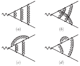
Figure 1: Feynman diagrams contributing to $c_{3}$. Straight and curly lines denote heavy quarks with mass $m$ and gluons, respectively.

Sample Feynman diagrams contributing to $c_{v}$ at the three-loop order are shown in Figure 1. After generating all relevant Feynman amplitudes and mapping them to scalar functions we use the program crusher [41] for the reduction to about 100 master integrals. Some of them are known analytically [35, 42] but the major part is evaluated numerically using the program FIESTA [19, 20, 21], which provides for each coefficient in the $\epsilon$ expansion an uncertainty originating from the Monte-Carlo integration. When summing the individual contributions these uncertainties are added in quadrature. Such an approach requires strong checks which are described in detail in [12, 36]. A very powerful check is provided by the change of the master integral basis. We employ the integral tables generated during the reduction procedure in order to re-express the master integrals, which are not known analytically, through different, in general more complicated ones. This transformation is done analytically for general space-time dimension $d$. In a next step the new master integrals are again evaluated with FIESTA and inserted into the new expression for $c_{v}$. For the final result we find excellent agreement within the uncertainties which is a strong check on the correctness of the result.

In the following we present the result specifying $N_{c}=3$ and $\mu=m$

$$c_{v}\approx 1-2.667\frac{\alpha_{s}^{(n_{l})}}{\pi}+\left(\frac{\alpha_{s}^{(n_{l})}}{\pi}\right)^{2}\left[-44.551+0.407n_{l}\right]$$ (10)

$$\mbox{}+\left(\frac{\alpha_{s}^{(n_{l})}}{\pi}\right)^{3}\Big{[}-2091(2)+120.66(0.01)\,n_{l}$$

$$\mbox{}-0.823\,n_{l}^{2}\Big{]}+\mbox{singlet terms}\,.$$

Results for individual colour coefficients and general values of $\mu$ can be found in [35, 12, 36].

3.2 Coulomb potential, $a_{3}$

In this subsection we summarize the potentials needed for top-quark pair production where our special emphasis lies on the three-loop corrections to the static potential. In momentum space the potential can be written in terms of operators expanded in $1/m$. Its colour-singlet projection reads

$$V({\bf p},{\bf p}^{\prime})=-{\cal V}_{C}(\alpha_{s})\frac{4\pi C_{F}\alpha_{s}}{{\bf q}^{2}}$$ (11)

$$\mbox{}+{\cal V}_{1/m}(\alpha_{s})\frac{\pi^{2}(4\pi)C_{F}\alpha_{s}}{m|{\bf q}|}+{\cal O}(1/m^{2})\,,$$

where for brevity only the first two terms are shown; the $1/m^{2}$ operators can be found in [6]. The coefficients of the operators are expanded in $\alpha_{s}$ where to N³LO the potential coefficient ${\cal V}_{C}(\alpha_{s})$ is needed to three-, ${\cal V}_{1/m}(\alpha_{s})$ to two-loop and the coefficient of the $1/m^{2}$ term to one-loop accuracy. Note that there is no tree-level contribution of order $1/m^{3}$.

The $1/m^{2}$ coefficients are known since long (see [6] for a detailed discussion). Also ${\cal V}_{1/m}$ has been computed more then ten years ago [43], however, only up to the constant term in the $\epsilon$ expansion. Since the potential loop-momentum integrals which have to be solved to obtain the corrections to the Green function $G(E)$ are divergent, the ${\cal O}(\epsilon)$ term of the two-loop correction to ${\cal V}_{1/m}$ is also required. It can be found in the Appendix of [44]. The three-loop correction to ${\cal V}_{C}$, commonly denoted $a_{3}$, has been computed by two independent groups [45, 46, 47]. The corresponding results shall be discussed in more detail in the following.

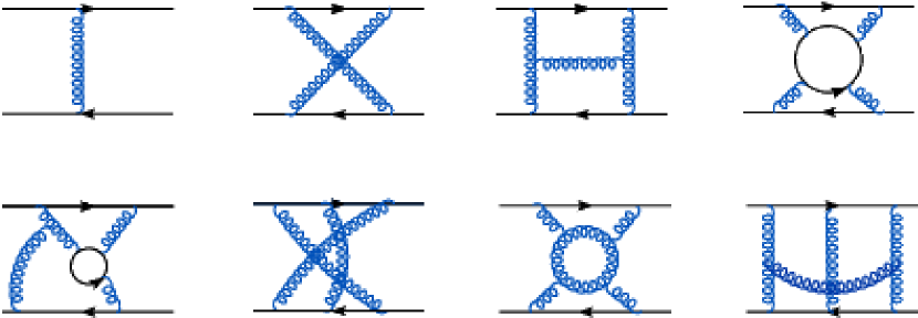
Figure 2: Sample Feynman diagrams contributing to the static potential at tree-level, one-, two- and three-loop order. Solid and curly lines represent quarks and gluons, respectively. In the case of closed loops the quarks are massless; the external quarks are heavy and treated in the static limit.

In Figure 2 sample Feynman diagrams contributing to ${\cal V}_{C}$ are shown. The external quarks are considered as heavy and thus for them the static approximation is applied. The only momentum scale in the problem is given by the momentum transfer $q$ between the quark and antiquark which has only non-vanishing space-like components. Furthermore, the static heavy-quark propagators have the form $1/(-v\cdot p-s_{i}i0)$ with $v\cdot p=p_{0}$ and $s_{i}=\pm 1$ and thus do not depend on $q$. As a consequence, any Feynman integral that contributes to $a_{3}$ can be mapped to one of the three graphs shown in Figure 3 where solid lines stand for usual massless propagators of the form $1/(-p^{2}-i0)^{a_{i}}$ and zigzag lines stand for static propagators which might also be raised to an integer index. In case the latter type of propagators is absent the integrals reduce to usual massless two-point functions, which can be treated with the help of MINCER [48]. Note, however, that the presence of the static lines significantly increases the complexity of the problem.

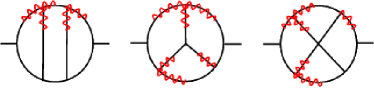
Figure 3: Families of Feynman integrals needed for the calculation of $a_{3}$. The solid lines correspond to relativistic massless propagators and the zigzag lines represents static propagators.

In general the integrals involve up to fifteen propagators (including an irreducible numerator). In order to simplify the reduction problem we apply in a first step partial fraction identities to arrive at various subfamilies of integrals with at most three linear propagators. Thus, any resulting integral is labelled by twelve indices one of which corresponds to an irreducible numerator and three indices correspond to linear propagators. As an example we show in Figure 4 the resulting families for the “Mercedes” graph of Figure 3.

Figure 4: Families with twelve indices (eleven propagators plus one scalar product) after applying partial fractioning to the “Mercedes” graph of Figure 3.

The next step is a reduction of all the Feynman integrals to master integrals by solving integration-by-parts relations [49]. This is done with the help of FIRE (Feynman Integral REduction) [50, 51, 52].

In total there are 41 master integrals which contribute to the three-loop static potential. Ten integrals have no static lines and are thus known since long [53, 54, 55]. Fourteen master integrals contain a massless one-loop insertion which can easily be integrated in terms of $\Gamma$ functions using standard formulae. As a result one obtains two-loop integrals where one of the indices has a non-integer exponent involving the space-time parameter $\epsilon=(4-d)/2$. Results for these integrals are shown in [56]. The 17 remaining integrals are more complicated and can only be computed in an expansion in $\epsilon$. Explicit results can be found in [57] (see also [58]). Actually, all but three coefficients in the $\epsilon$ expansion could be computed analytically. The three numerical results are known to a sufficiently high precision for all foreseeable phenomenological applications.

An important check for the correctness of the calculation is the use of a general QCD gauge parameter [46]. Note that the computational price one has to pay is quite high: a rough estimate of the complexity based on the number of integrals which have to be reduced to masters shows that the linear $\xi$ term is about seven times and the $\xi^{3}$ term even 18 times more complicated than the Feynman gauge expression. Let us mention that nevertheless all occurring integrals could be reduced with the help of FIRE.

We write the perturbative expansion of ${\cal V}_{C}$ in the form

$${\cal V}_{C}(\alpha_{s}) = {\cal V}_{C}^{(0)}+\frac{\alpha_{s}}{4\pi}{\cal V}_{C}^{(1)}+\bigg{(}\frac{\alpha_{s}}{4\pi}\bigg{)}^{\!2}{\cal V}_{C}^{(2)}$$ (12)

$$\mbox{}+\bigg{(}\frac{\alpha_{s}}{4\pi}\bigg{)}^{\!3}{\cal V}_{C}^{(3)}+O(\alpha_{s}^{4})\,.$$

Up to two-loop order the coefficients ${\cal V}_{C}^{(i)}$ are finite, however, at three loops an infrared divergence occurs [59], which is related to ultraviolet divergences in the calculation of the ultrasoft corrections. It is convenient to subtract these divergences in $V({\bf p},{\bf p}^{\prime})$ and add them back to the ultrasoft calculation. In the case of the Coulomb potential the infrared divergence is cancelled after adding the $\overline{\rm MS}$ counterterm

$$\delta V_{C,c.t.} = \frac{\alpha_{s}C_{F}}{6\epsilon}C_{A}^{3}\frac{\alpha_{s}^{3}}{{\bf q}^{2}},$$ (13)

to $V({\bf p},{\bf p}^{\prime})$ in (11). One finally arrives at

$${\cal V}_{C}^{\,(0)} = 1,$$

$${\cal V}_{C}^{\,(1)} = \bigg{[}\bigg{(}\frac{\mu^{2}}{{\bf{q}}^{2}}\bigg{)}^{\!\epsilon}-1\bigg{]}\,\frac{\beta_{0}}{\epsilon}\,+\bigg{(}\frac{\mu^{2}}{{\bf{q}}^{2}}\bigg{)}^{\!\epsilon}\,a_{1}(\epsilon),$$

$${\cal V}_{C}^{\,(2)} = a_{2}+\left(2a_{1}\beta_{0}+\beta_{1}\right)\ln\frac{\mu^{2}}{{\bf{q}}^{2}}+\beta_{0}^{2}\ln^{2}\frac{\mu^{2}}{{\bf{q}}^{2}},$$

$${\cal V}_{C}^{\,(3)} = a_{3}+\left(2a_{1}\beta_{1}+\beta_{2}+3a_{2}\beta_{0}+8\pi^{2}C_{A}^{3}\right)$$ (14)

$$\mbox{}\times\ln\frac{\mu^{2}}{{\bf{q}}^{2}}+\left(\frac{5}{2}\beta_{0}\beta_{1}+3a_{1}\beta_{0}^{2}\right)\ln^{2}\frac{\mu^{2}}{{\bf{q}}^{2}}$$

$$\mbox{}+\beta_{0}^{3}\ln^{3}\frac{\mu^{2}}{{\bf{q}}^{2}}\,.$$

Note the $\ln\mu^{2}$ term in ${\cal V}_{C}^{\,(3)}$ not associated with the QCD beta function is the remnant of the infrared divergence. We refrain from providing explicit results for $a_{1}$ and $a_{2}$ which can be found in the literature [60, 61, 62, 63, 43], even including higher order terms in $\epsilon$ [45, 6]. The result for $a_{3}$ reads [45, 46, 47]

As mentioned above, some of the ingredients entering $a_{3}$ are only known numerically; they enter four of the colour factors in (LABEL:eq:a3) and are taken from [46, 57]. Also parts of the N⁴LO Coulomb potential are known [64], but not needed for the third-order cross section calculation. The two- and three-loop corrections to the static potential of heavy quarks in the colour-octet state have been computed in [65] and [66], respectively.

3.3 Third-order potential corrections to the PNRQCD correlation function

Once the matching coefficients of NRQCD and PNRQCD are determined, the correlation function $G(E)$ defined in (8) has to be calculated to the third order in PNRQCD perturbation theory. Since the leading-order Coulomb potential $V_{0}(r)$ in (4) is part of the unperturbed Lagrangian, the position-space propagator is the matrix element $G_{0}({\bf{r}},{\bf{r}}^{\prime};E)=\langle{\bf{r}}|\hat{G}_{0}(E)|{\bf{r}}^{\prime}\rangle$ of the Green operator $\hat{G}_{0}(E)=[H_{0}-E-i\epsilon]^{-1}$. The propagator propagates a heavy quark-antiquark pair, and ${\bf{r}}$ refers to the separation of the heavy quark-antiquark fields. Since one usually works in the centre-of-mass (cms) frame, the cms motion is irrelevant. The unperturbed theory is not free, but it is still exactly solvable, since $H_{0}$ is the Hamiltonian of the Coulomb problem. An explicit expression for the Coulomb Green function in terms of Laguerre polynomials $L_{s}^{(2l+1)}$ and a partial-wave decomposition is [67, 68]

The corrections consist of potential contributions from single and multiple insertions of perturbation potentials $\delta V_{k}$ of order $\mathcal{O}(v^{k})$ relative to the leading-order Coulomb potential, which arise from radiative corrections to the Coulomb potential and further non-Coulomb potentials such as ${\cal V}_{1/m}$ in (11). Starting from the third order, there is an ultrasoft contribution, $\delta^{us}G(E)$, which is briefly discussed in Section 3.4.

The first term on the right-hand side of (LABEL:masterthirdorder) represents the triple insertion of the one-loop correction $\delta V_{1}$ to the Coulomb potential. The presence of four propagators of the form (LABEL:eq:CoulombGreen) turns this into a complicated expression. However, all the integrations are ultraviolet-finite, and this allows the triple insertion to be converted into sums that can be evaluated numerically as done in [69]. Instead of computing order by order multiple insertions of $\delta V_{1}$, one can also include $\delta V_{1}$ into the unperturbed Lagrangian and solve for the Green function of the associated Schrödinger problem numerically, which sums the insertions of $\delta V_{1}$ to all orders. The comparison of the two approaches performed in [69] shows that good convergence of the PNRQCD expansion to the exact result is only achieved when the renormalization scale $\mu$ is larger than 30 GeV. Somewhat surprisingly PNRQCD perturbation theory already breaks down at scales larger than the natural scale of the inverse Bohr radius, but works when $\mu$ is chosen closer to the hard scale. The explicit verification of this scale choice by comparison with the exact result, which is only possible for the Coulomb potential, lends support to the scale choice that will be made in the evaluation of the full third-order cross section below.

The second and third term on the right-hand side of (LABEL:masterthirdorder) are associated with the single insertion of third-order potentials, such as the three-loop correction to the Coulomb potential discussed in the previous subsection, and the double insertion of a second-order potential together with the one-loop correction to the Coulomb potential. While algebraically simpler than the triple insertion, they turn out to be more difficult to evaluate. The reason is that potentials more singular than $1/r$ as $r\to 0$ cause ultraviolet divergences of the potential integrals, which have to be consistently calculated and factorized in dimensional regularization, so that the divergences cancel with the matching coefficients and the finite term is correctly computed. At the same time, a calculation of the all-order diagrams summed by PNRQCD perturbation theory in $d$ dimensions is not possible, since the propagator (LABEL:eq:CoulombGreen) is known only in four dimensions.

The calculation of these non-Coulomb potential terms is described in detail in [70]. (The corresponding result for the bound-state parameters has already been presented in [71] and for the Green function in [72], though no details were given in this work.) Here we discuss as an example the single insertion of the $1/r^{2}$ potential to illustrate the strategy of the calculation. In momentum space the $d$-dimensional $1/r^{2}$ potential ${\cal V}_{1/m}$ is of the form $w(\epsilon)/({\bf q}^{2})^{1/2+a\epsilon}$, where $a$ is an integer. A single insertion is an integral

The advantage of this expression is that it avoids the need to calculate in $I[x+a\epsilon]$ the $a$-independent $\mathcal{O}(\epsilon)$ terms, since they drop out in the difference in brackets in the first term. These terms would indeed be diificult to obtain. The second term is multiplied by a finite series, hence the $\mathcal{O}(\epsilon)$ term of $I[x]$ is never required to obtain the finite part of $J$ as $\epsilon\to 0$.

The single insertion of the $1/r^{2}$ potential generates ultraviolet $1/\epsilon$ poles from the integration over the potential loop momenta, which are related to the singularities in the dimensionally regulated hard current matching coefficients, and which have to be properly factorized. Power counting shows that the insertion has an overall divergence coming from diagrams with less then two gluon exchanges, and a vertex subdivergence, when there is no gluon exchange between the external vertex and the potential insertion. To accomplish the correct factorization, we divide the integral into four different parts (and show the corresponding diagrams below):

Similar notation applies to the counterterm-including insertion function $J$. The first two terms map to two- and three-loop diagrams, which carry an overall divergence and a divergence in the vertex subgraph(s) without gluon exchanges. The fourth term represents a sum of diagrams to all orders, but is finite. The third term has a divergence in the left vertex subgraph and all-order summation to the right of the potential insertion, where the notation “$\,>\!1$” refers to all ladder diagrams summed by $\hat{G}_{0}(E)$ with more than one gluon exchange.

The calculation of the first two parts is straightforward, since it involves only ordinary, solvable, dimensionally regularized two- and three-loop diagrams. Nevertheless, the divergent part must be properly factorized. To be explicit, the two-loop integral for diagram (a) evaluates to

where the $1/\epsilon$ pole parts now multiply the $d$-dimensional zero-exchange Coulomb Green function.

Contributions such as part c, which have subdivergences and represent all-order graphs are the most complicated ones, since $G_{0}^{(>1ex)}(E)$ that appears to the right of the insertion is not known in $d$-dimensions. The strategy consists of isolating the subdivergence at the integrand level, so that it can be factorized without ever requiring an explicit representation of $G_{0}^{(>1ex)}(E)$. The finite remainder can then be evaluated in four dimensions. This strategy always works, because the divergences can only arise from subdiagrams with a finite number of loops. This must be so, since the divergences must cancel with infrared divergences in the matching coefficients, which are computed in fixed-order perturbation theory. On the technical level, the finiteness of ladder diagrams with potential insertions once there are sufficiently many ladder rungs follows from the fact that every rung reduces the degree of divergence. For explicit results for the other parts of $J[\frac{1}{2}+a\epsilon;w(\epsilon)]$ we refer to [70]. An important consistency check is that the factored divergent parts of $J_{a}$, $2J_{b}$ and $2J_{c}$ are all the same. This is necessary for the sum of all contributions to add to a term proportional to the full Green function $G_{0}(E)=G_{0}^{(0ex)}(E)+G_{0}^{(1ex)}(E)+G_{0}^{(>1ex)}(E)$. That is, for the sum of all parts we have

as is required for cancelling the divergent part with the hard matching coefficient multiplying $G_{0}(E)$. The method also applies to double insertions, where some expressions require the factorization of a $1/\epsilon$ pole multiplying the single insertion of the NLO Coulomb potential. In the end, one verifies the cancellation of all poles in the sum of all terms, and evaluates the remainder numerically.

3.4 Ultrasoft correction

A contribution from the ultrasoft loop momentum region has to be taken into account for the first time at the third order in perturbation theory. The ultrasoft correction $\delta^{us}G(E)$ to (LABEL:masterthirdorder) is technically and conceptually the most complicated contribution to the third-order correction to $G(E)$, since its (sub) divergence structure is rather involved and the integrals are more difficult. The correction to the Green function relevant to the top-pair cross section was computed in [73], with the subtraction scheme already developed in [74] to determine the bound-state residues. In this subsection we want to summarize the most important features.

The ultrasoft interaction terms in the PNRQCD Lagrangian (LABEL:eq:pnrqcd) relevant to third order are given by

$$g_{s}\psi^{\dagger}(x)\big{[}A_{0}(t,{\bf{0}})-{\bf{x}}\cdot{\bf{E}}(t,{\bf{0}})\big{]}\psi(x)$$

$$\mbox{}+g_{s}\chi^{\dagger}(x)\big{[}A_{0}(t,{\bf{0}})-{\bf{x}}\cdot{\bf{E}}(t,{\bf{0}})\big{]}\chi(x).$$ (30)

The leading $A_{0}(t,{\bf{0}})$ couplings can be removed by a redefinition of the heavy-quark fields with a time-like Wilson line, which modifies the production current. The Wilson lines cancel for colour-singlet currents, hence the $A_{0}(t,{\bf{0}})$ couplings have no effect on top-pair production in $e^{+}e^{-}$ collisions. Note that ${\bf{x}}\sim 1/v$ and $g_{s}{\bf{E}}\sim v^{9/2}$ for ultrasoft gluon fields and thus the remaining chromoelectric dipole interaction is suppressed by $v^{3/2}$ relative to the kinetic term in the action. Two ultrasoft interaction vertices are required to form an ultrasoft loop, from which it follows that the leading ultrasoft contribution arises only at the third order.

Employing the Feynman rule for the ${\bf{x}}\cdot{\bf{E}}(t,{\bf{0}})$ vertex, the ultrasoft correction to the Green function can be expressed in the form

with the understanding that one picks up only the pole at $k^{0}=|{\bf{k}}|-i\epsilon$ in the gluon propagator. However, this expression cannot be used in practice, because it is ultraviolet divergent. Instead, one reverts the derivation of the chromoelectric dipole interaction and uses the Feynman rules for the threshold-expanded NRQCD momentum-space diagrams together with dimensional regularization.

The ultrasoft correction $\delta^{us}G(E)$ has ultraviolet divergences from the integral over the three-momentum ${\bf{k}}$ of the ultrasoft gluon, and from the subsequent potential loop integrations. The former take the form of a single insertion of a third-order potential and of a one-loop correction to the coefficient $d_{v}$ of the $\mathcal{O}(v^{2})$ suppressed derivative current. Note that ultraviolet divergence has to be regularized in dimensional regularization to be consistent with the calculation of potential insertions and hard-matching coefficients. For this reason it is convenient to introduce appropriate subtraction terms to cancel the ultrasoft subdivergences, which leads to [74, 6]

where $\delta V_{c.t.}$ represents the potential subtraction, and $\delta U$ is the ultrasoft insertion (containing the octet Green function). The first line of (LABEL:eq:defUS) is related to the renormalization of the $\mathcal{O}(v^{2})$ suppressed vector current. In fact, $\delta d_{v}^{\rm div}$ contains the infrared divergence that was subtracted to obtain the finite expression for $d_{v}$ in (7). The divergences in the second line are associated with potential insertions. The counterterm (13) that is needed to make the three-loop Coulomb potential finite after coupling renormalization is contained in $\delta V_{c.t.}$ above. The remaining divergences of (LABEL:eq:defUS) from the potential loop integrations are associated with the three-loop hard matching coefficient $c_{v}$ and isolated as explained in [74]. The final result is then evaluated by a combination of analytical and numerical methods.

3.5 Third-order cross section

In this subsection we put all third-order corrections together and briefly discuss their numerical effect on the production cross section of top-quark pairs (see also [75]). We restrict ourselves to pure QCD corrections and furthermore only consider S-wave contributions.

The (normalized) total cross section is given by (5). We parametrize $R$ in terms of the potential subtracted (PS) mass [76]. This avoids the infrared sensitivity of the pole mass [77, 78], which would otherwise prohibit a mass determination with accuracy below $\Lambda_{\rm QCD}$. The PS mass is related to the pole mass via

$$m_{t}^{\rm PS}=m_{t}-\delta m_{t}(\mu_{f}),$$ (33)

where $\delta m_{t}(\mu_{f})$ is obtained from the static potential solving the following integral

$$\delta m_{t}(\mu_{f})=-\frac{1}{2}\int_{|{\bf{q}}\,|<\mu_{f}}\frac{{\rm d}^{3}{\bf{q}}}{(2\pi)^{3}}V({\bf{q}}\,)\,.$$ (34)

The factorization scale $\mu_{f}$ is part of the definition of the PS mass. In the following we set it to $\mu_{f}=20$ GeV. To obtain $\delta m_{t}(\mu_{f})$ to N³LO [69] the three-loop coefficient of the static potential (cf. Section 3.2) is needed.

We are now in the position to numerically evaluate (5) where our default input parameters are given by

$$\alpha_{s}(M_{Z}) = 0.1184\,,$$

$$m_{t}^{\rm PS} = 171.3\leavevmode\nobreak\ \mbox{GeV}\,,$$

$$\Gamma_{t} = 1.4\leavevmode\nobreak\ \mbox{GeV}\,.$$ (35)

As the central value for the renormalization scale we adopt $\mu=80$ GeV.

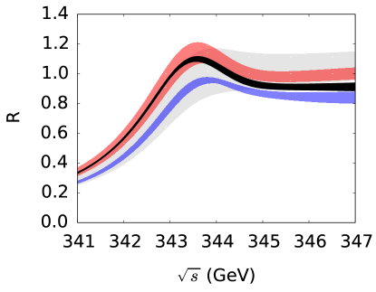
Figure 5: $R$ as a function of the $e^{+}e^{-}$ centre-of-mass energy in the threshold region. LO, NLO, NNLO and N³LO results are shown in grey, blue (lowest band at $\sqrt{s}=347\,\mbox{GeV}$), red and black where the bands indicate the uncertainty due to scale variation.

In Figure 5 the normalized total cross section is shown as a function of $\sqrt{s}$ in the threshold region. The bands are obtained by simultaneous variation of the renormalization and factorization scale between $50$ and $350$ GeV. After the inclusion of the third-order corrections one observes a dramatic stabilization of the perturbative prediction, in particular in and below the peak region, where most of the sensitivity to the top-quark mass comes from. In fact, the N³LO band is entirely contained within the NNLO one in this region. This is different above the peak position where a sizable negative correction is observed when going from NNLO to N³LO. For example, 2 GeV above the peak this amounts to about $-10\%$.

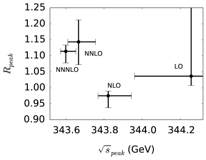
Figure 6: LO, NLO, NNLO and N³LO results for the height (vertical axis) and position (horizontal axis) of the peak. The error bands originate from scale variation and uncertainties in $\alpha_{s}$.

It is interesting to have a closer look at the position and height of the peak. Figure 6 shows the peak height and its position at LO, NLO, NNLO and N³LO where the error bars reflects the uncertainty due to the scale and $\alpha_{s}$ variation, which are added in quadrature. In the position of the peak one observes a relatively big jump from LO to NLO of about 400 MeV, and from NLO to NNLO of approximately 150 MeV which reduces to only 50 MeV from NNLO to N³LO. Furthermore, the NNLO and N³LO uncertainty bands show a significant overlap. The uncertainty of the peak position amounts to about 70 MeV, 60 MeV and 30 MeV at NLO, NNLO and N³LO. As far as the height is concerned there are big jumps from LO to NLO and NLO to NNLO, however, the N³LO correction stabilizes the perturbative series and a shift below 3% is observed.

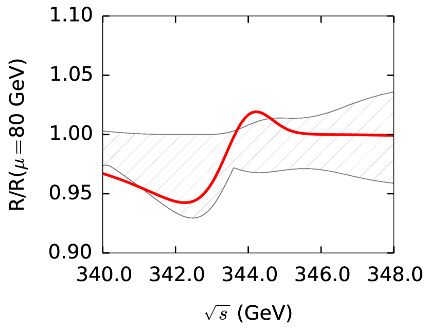
Figure 7: N³LO corrections to $R(s)$ normalized to its value for $\mu=80$ GeV where the band corresponds to scale variation between $50$ and $350$ GeV. For the (red) solid curve the input value for $m_{t}^{\rm PS}$ in (35) by $+50$ MeV.

In Figure 7 we study the sensitivity of the total cross section on the variation of the top-quark mass. This is done by normalizing the N³LO band of Figure 5 to the result obtained for $\mu=80$ GeV. The hatched band in Figure 7 represents the theoretical uncertainty of this normalized quantity. The red curve in Figure 7 is obtained by adopting $\mu=80$ GeV and shifting $m_{t}^{\rm PS}$ by $+50$ MeV. Above threshold basically no effect is observed. However, the strong variation of the cross section below threshold implies a several percent effect even for such a small variation of $m_{t}^{\rm PS}$, and provides a handle for the precise determination of the top-quark mass. From Figure 7 one may expect a precision of about $50\,\mbox{MeV}$, and it is obvious that the small theoretical uncertainty after including the third-order corrections to $R$ is crucial to reach this goal. Similar results are obtained for variations of other parameters like the strong coupling constant and the top-quark width [75].

Finally we mention that (almost complete) next-to-next-to-leading logarithmic predictions for the total cross section have been obtained [79, 80]. In this approach, the logarithmically enhanced terms in $v$ of the third-order correction are included, but not the sizable “constant” terms. On the other hand, logarithms of $v$ are summed to all orders. At first glance there appears to be good agreement with our N³LO results. However, a detailed comparison of the different terms included in the two approaches is required to determine whether the agreement is more than coincidental.

3.6 Further results

With the third-order QCD corrections to the dominant S-wave production mode completed and uncertainties under good control, attention must be paid to other corrections that may be less challenging from the technical perspective, but important phenomenologically. There are QED and electroweak corrections, where we count $\alpha_{\rm em}\sim\alpha_{\rm EW}\sim\alpha_{s}^{2}\sim v^{2}$; Higgs boson contributions; production of $t\bar{t}$ in a P-wave state; non-resonant contributions to the physical final state $W^{+}W^{-}b\bar{b}$; and a consistent treatment of initial-state radiation with controlled dependence on the factorization scheme for the initial-state electron distribution function. We discuss some of these items below (see [81, 82] for a general discussion of initial-state radiation in this context and some relevant formalism).

3.6.1 P-wave contribution

The P-wave contribution arises from the axial-vector coupling of the $Z$-boson to the $t\bar{t}$ pair. Since the imaginary part of the axial-vector polarization function $\Pi^{(a)}(q^{2})$ is $\mathcal{O}(v^{2})$ suppressed in the non-relativistic limit, a NLO calculation of $\Pi^{(a)}(q^{2})$ in PNRQCD results in a third-order contribution to the total top-pair production cross section near threshold. The NLO calculation was performed in [83]. The NLO correction stabilizes the scale dependence, but the result is ambiguous until a scheme is defined to combine the resonant with non-resonant contributions, see Section 3.6.3 below. However, the P-wave contribution is always a very small contribution, below 1%, to the total cross section.

3.6.2 Higgs contributions

The Higgs contributions are of particular interest, since they provide sensitivity of the cross section $\sigma(e^{+}e^{-}\to t\bar{t}+X)$ to the top-quark Yukawa coupling to the Higgs boson. The dependence originates from Higgs exchange between the produced top quarks (potential region), and from radiative corrections to the production vertex (hard region). These effects are incorporated into the PNRQCD framework via modifications of the vector current which result from simultaneously integrating out the top quark and the Higgs boson, assuming $M_{H}\sim m_{t}$ for power counting. Furthermore, a new operator occurs in the effective theory, which in momentum space is given by [38]

$$\delta{\cal L}_{H} = \frac{\alpha\pi m_{t}^{2}}{s_{W}^{2}M_{W}^{2}M_{H}^{2}},$$ (36)

where $s_{W}$ is the sine of the weak mixing angle and $M_{W}$ is the $W$ boson mass. In coordinate space, this is equivalent to a delta function potential that approximates the short-range Yukawa potential. If we employ the counting rule $\alpha\sim\alpha_{s}^{2}$ it is easy to see that $\delta{\cal L}_{H}$ gives contributions which are parametrically of the same order as the ones from the third-order PNRQCD Lagrangian.

We parametrize electroweak corrections to the matching coefficient $c_{v}$ as

$$c_{v} = 1+\frac{\alpha}{\pi s_{W}^{2}}c_{v}^{\rm ew}+\frac{\alpha\alpha_{s}}{\pi^{2}s_{W}^{2}}C_{F}c_{v}^{\rm mix}+\ldots\,,$$ (37)

where the the ellipses stand for QCD corrections which can be found in (10). The complete one-loop electroweak corrections to the matching coefficient $c_{v}^{\rm ew}$ have been computed in [37]. The Higgs boson contribution can be cast in the form

$$c_{v}^{H,\rm ew} = \frac{m_{t}^{2}}{M_{W}^{2}}\Bigg{[}\frac{3y_{H}^{2}-1}{12y_{H}^{2}}-\frac{2-9y_{H}^{2}+12y_{H}^{4}}{48y_{H}^{4}}\ln y_{H}^{2}$$ (38)

$$\mbox{}-\frac{(-2+5y_{H}^{2}-6y_{H}^{4})}{24y_{H}^{2}}$$

$$\mbox{}\times\frac{\sqrt{4y_{H}^{2}-1}}{y_{H}^{2}}\arctan{\sqrt{4y_{H}^{2}-1}}\Bigg{]}\,,$$

where $y_{H}=m_{t}/M_{H}$ and $m_{t}$ is the on-shell top-quark mass. Mixed contributions of order $\alpha\alpha_{s}$ involving the Higgs boson have been computed in [38] where various expansions have been considered. For $M_{H}\approx 125$ GeV an expansion around $m_{t}\approx M_{H}$ leads to the best results for $c_{v}^{H,\rm mix}$, which can be written as

$$c_{v,1b}^{H,\rm mix}=\frac{m_{t}^{2}}{M_{W}^{2}}\Bigg{[}\frac{\pi^{2}}{8}\left(1-y_{H,1b}\right)\ln{\frac{m_{t}^{2}}{\mu^{2}}}-5.760$$ (39)

$$\mbox{}+5.533y_{H,1b}-0.171y_{H,1b}^{2}+0.0124y_{H,1b}^{3}$$

$$\mbox{}+0.0304y_{H,1b}^{4}+0.0296y_{H,1b}^{5}+\ldots\Bigg{]}\,,$$

with $y_{H,1b}=(1-y_{H}^{2})$.

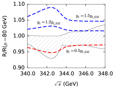
Figure 8: N³LO corrections to $R(s)$ normalized to its value for $\mu=80$ GeV where the band corresponds to scale variation between $50$ and $350$ GeV. For the dashed curves the input value for the top Yukawa coupling in the $t\bar{t}H$ vertex is rescaled relative to the SM value by a factor 1.5, 1.2, 0.5 (from top to bottom) while keeping the top-quark mass at its input value (35). The central value to which the variation is normalized includes the SM Higgs contributions.

The PNRQCD computation of the Higgs contributions to $\sigma(e^{+}e^{-}\to t\bar{t}+X)$ has been performed in [87] and results in corrections at the $10\%$ level as expected from the discussion of the corrections to the bound-state residue [38]. Higgs contributions of order $\alpha\alpha_{s}$ clearly have to be incorporated in order to reach a precision at the few-percent level.

Figure 8 shows the effect of a modification of the top-Yukawa coupling relative to its SM value of the top-pair production cross section near threshold in a format similar to Figure 7. Comparing the width of the uncertainty band to the shift of the curves provides a first estimate of how well the top-Yukawa coupling can be constrained at a future $e^{+}e^{-}$ collider before the cms energy for open $t\bar{t}H$ production is reached [87].

3.6.3 Non-resonant contributions

The most important piece that is still missing for a realistic prediction of the total cross section is related to the fact that the top quark decays rapidly. The measurement of top-pair production near threshold really refers to the measurement of $e^{+}e^{-}\to W^{+}W^{-}b\bar{b}$ with cms energy $\sqrt{s}$ near $4m_{t}^{2}$. The pure QCD contribution, which we referred to above, is defined by the polarization function evaluated in the complex energy plane with the prescription $E\to E+i\Gamma_{t}$.

The limitations of this approximation manifest themselves within the (NR)QCD calculation itself. The current correlation function $G(E)$ exhibits an uncancelled ultraviolet divergence from an overall divergence of the form $[\delta G(E)]_{\rm overall}\propto\alpha_{s}E/\epsilon$ in dimensional regularization [73]. Since $E$ acquires an imaginary part $\Gamma_{t}\sim m_{t}\alpha_{\rm EW}$ through the above prescription, the divergence survives in the cross section,

$$\mbox{Im}\,[\delta G(E)]_{\rm overall}\propto m_{t}\times\frac{\alpha_{s}\alpha_{\rm EW}}{\epsilon}.$$ (40)

The divergence appears first at NNLO (since at LO, $G(E)\sim v\sim\alpha_{s}$), and results in dependence on an additional regularization scale $\mu_{w}$ after subtraction. A consistent calculation therefore requires that one considers the process $e^{+}e^{-}\to W^{+}W^{-}b\bar{b}$ within unstable-particle effective theory [88, 89] including the effects of off-shell top quarks and processes that produce the $W^{+}W^{-}b\bar{b}$ final state with no or only one intermediate top-quark line. The physical cross section is then the sum of two terms,

$$\sigma_{e^{+}e^{-}\to W^{+}W^{-}b\bar{b}}=\underbrace{\sigma_{e^{+}e^{-}\to[t\bar{t}]_{\rm res}}(\mu_{w})}_{\mbox{\footnotesize pure (NR)QCD}}$$

$$\hskip 22.76228pt+\,\sigma_{e^{+}e^{-}\to W^{+}W^{-}b\bar{b}{}_{\rm nonres}}(\mu_{w}).$$ (41)

Both terms separately have a “finite-width scale dependence”, and only the sum is well-defined. The calculation of the non-resonant part has been performed so far only at NLO [90, 91], including the possibility to apply invariant-mass cuts on the top decay products. Parts relevant to NNLO are known [91, 92, 93, 94], but the complete computation is still missing. For a further discussion of non-resonant contributions and unstable-particle effective theory we refer to the review [95] in this volume.

4 Threshold resummation in hadronic collisions

The production of top-quark pairs, and pairs of heavy particles in general, in proton-proton (LHC) or proton-antiproton (Tevatron) collisions is different from $e^{+}e^{-}$ annihilation in two important aspects. First, the centre-of-mass energy of the colliding partons is not fixed. Non-relativistic theory is strictly relevant only in the kinematic region of small invariant mass of the heavy-particle pair near the kinematic limit. Second, the initial-state particles are coloured, so that the heavy-particle pair can be produced in different colour states. This implies that soft gluon effects are much more important than in $e^{+}e^{-}$ annihilation, both due to initial-state radiation, and due to the coupling to the coloured final state. (Following standard terminology, what we call “soft” in this section, refers to the ultrasoft region in previous sections.) In this section we discuss the theoretical formalism that brings together non-relativistic theory with the theory of soft-gluon resummation, the latter having been developed first for Drell-Yan production [96, 97] and then extended to di-jets or pairs of heavy particles [98, 99, 100, 101, 102, 103, 104]. We then consider the invariant-mass distribution of hadronically produced top pairs, and the total cross section for top and superpartner particle pairs.

4.1 Joint soft and Coulomb resummation

The theoretical quantities of interest are the hard-scattering cross sections $\hat{\sigma}$ for the partonic subprocesses

$$p(k_{1})p^{\prime}(k_{2})\rightarrow H(p_{1})H^{\prime}(p_{2})+X$$ (42)

with $pp^{\prime}\in\{qq,q\bar{q},\bar{q}\bar{q},gg,gq,g\bar{q}\}$, when the partonic centre-of-mass energy $\hat{s}$ is close to $4M^{2}\equiv(m_{H}+m_{H^{\prime}})^{2}$, such that $\beta=(1-4M^{2}/\hat{s})^{1/2}$ is small. The two heavy particles $H$, $H^{\prime}$ can be in arbitrary, not necessarily identical colour representations $R$, $R^{\prime}$.

The expansion of $\hat{\sigma}$ contains enhanced terms of the form $(\alpha_{s}\ln^{2}\beta\,)^{n}$, primarily (but not exclusively) related to soft gluon effects, and the “Coulomb singularities” $(\alpha_{s}/\beta)^{n}$, which both cause a breakdown of the perturbation expansion for small $\beta$. Although the power-like Coulomb singularities are formally stronger than the logarithmic soft-gluon effects, the importance of one or the other effect depends on the initial state (quark vs. gluon) and colour of the final state (for instance, singlet vs. octet). Joint soft and Coulomb resummation [105, 106] concerns the question whether both effects can be resummed simultaneously.

4.1.1 Factorization

This is a non-trivial issue, since the energy of soft gluons is of the same order as the kinetic energy $M\beta^{2}$ of the heavy particles produced. Soft-gluon lines may therefore connect without parametric suppression to the heavy-particle propagators in between the Coulomb ladder rungs, as well as to the Coulomb gluons itself (by virtue of the gluon self-coupling), impeding the standard factorization arguments that assume either no couplings to the final state, or to the energetic initial-state particles.

Factorization was investigated in [105, 106], where it was shown that the partonic cross section factorizes into three separate contributions, related to hard, soft and Coulomb effects. The latter two are coupled only through a convolution in an energy variable $\omega$, which roughly speaking accounts for the fact that near threshold the production of the heavy particle pair is sensitive to the small amount of energy radiated into soft gluons. The factorization formula reads

Here $E=\sqrt{\hat{s}}-2m_{t}$ is the energy relative to the production threshold. Referring to [106] for the derivation, we explain here the elements of the formula and properties of the effective interactions that lead to this simple form. The formula as written applies to the total cross section. A similar result without convolution integral holds for the distribution in the $HH^{\prime}$ invariant mass.

The first factor $H^{i}_{pp^{\prime}}(M,\mu)$ accounts for the short-distance production of $HH^{\prime}$. It depends on the masses of the heavy particles, the partonic initial state, but not on the small scales $E$ and $M\beta$ in the problem. The superscript $i$ refers to a colour decomposition to be discussed below. The function $J_{R_{\alpha}}(E)$ accounts for the non-relativistic effects from the potential region and coincides with the zero-distance Coulomb Green function $G(E)$, generalized to the case of unequal-mass particles and an arbitrary irreducible SU(3) representation. At leading order, this is easily accomplished by replacing $m$ by the reduced mass, and the colour-singlet coefficient $C_{F}$ of the Coulomb potential by $-D_{R_{\alpha}}$. $D_{R_{\alpha}}$ is determined by

$${\bf T}^{(R)b}_{a_{1}c_{1}}{\bf T}^{(R^{\prime})b}_{a_{2}c_{2}}P^{R_{\alpha}}_{c_{1}c_{2}a_{3}a_{4}}=D_{R_{\alpha}}P^{R_{\alpha}}_{\{a_{1}a_{1}a_{3}a_{4}\}},$$ (44)

where $P^{R_{\alpha}}_{a}$ projects on the irreducible representation $R_{\alpha}$ in the tensor product $R\otimes R^{\prime}$, and $T^{(R)}$ are the SU(3) generators in representation $R$. Finally, $W^{R_{\alpha}}_{i}(\omega,\mu)$ is the soft-gluon function in the representation $R_{\alpha}$.

Eq. (LABEL:eq:fact) holds up to corrections ${\cal O}(\beta^{2})$ for the total cross section near threshold. Within this approximation the interactions of soft gluons with collinear and non-relativistic particles take a particularly simple form, which is essential for proving factorization. The coupling of soft gluons to an energetic initial-state quark with four-momentum in the light-like $n$ direction is given by the term

$$\bar{\xi}_{c}(x)\,ig_{s}n\cdot A_{s}(x_{+})\,\frac{\not\!\bar{n}}{2}\,\xi_{c}(x),$$ (45)

in the position-space SCET Lagrangian, which is equivalent to the eikonal approximation. Here $\xi_{c}$ denotes the $n$-collinear quark field, and $\bar{n}$ is another light-like vector with $n\cdot\bar{n}=2$. It is important that only the $n\cdot A_{s}$ component appears, and the soft field is evaluated at the point $x_{+}^{\mu}=(\bar{n}\cdot x/2)\,n^{\mu}\equiv x_{-}n^{\mu}$ due to the light-cone multipole expansion [107, 108]. This allows the soft-gluon coupling to be removed from the Lagrangian by performing the field redefinition $\xi_{c}(x)=S^{(3)}_{n}(x_{-})\xi_{c}^{(0)}(x)$ [109], where

$$S^{(R)}_{n}(x)=\mbox{P}\exp\left[ig_{s}\!\int_{-\infty}^{0}\!\!\!dt\,n\cdot A^{c}_{s}(x+nt){\bf T}^{(R)c}\right]$$ (46)

denotes a light-like, soft Wilson line for a particle in the representation $R$ of SU(3). Similar results apply to initial-state gluons. The leading soft-gluon interaction with the non-relativistic fields for $H$ and $H^{\prime}$,

$$\psi^{\dagger}(x)\,ig_{s}A_{s}^{0}(x_{0})\,\psi(x)+\psi^{\prime\,\dagger}(x)\,ig_{s}A_{s}(x_{0})\,\psi^{\prime}(x),$$ (47)

involves only the $A_{0}$ fields at point $(x_{0},{\bf{0}}\,)$, and therefore can be removed by $\psi(x)=S^{(R)}_{w}(x_{0})\psi^{(0)}(x)$, where $w=(1,{\bf{0}}\,)$ is a time-like four-vector, and

$$S^{(R)\dagger}_{w}(x)=\mbox{P}\exp\left[ig_{s}\!\!\int_{0}^{\infty}\!\!\!dt\,w\cdot A^{c}_{s}(x+wt)\,{\bf T}^{(R)c}\right]$$ (48)

is the corresponding Wilson line. The decoupling of soft gluons from the Coulomb gluons in ladder diagrams now follows from the identity $S_{w}^{(R)\dagger}{\bf T}^{(R)a}S_{w}^{(R)}=S_{w;ab}^{(8)}{\bf T}^{(R)b}$, which in turn implies $\left[\psi^{\dagger}{\bf T}^{(R)a}\psi\right]\!(x+{\bf{r}}\,)=S_{w;,ab}^{(8)}(x_{0})\left[\psi^{\dagger(0)}{\bf T}^{(R)b}\psi^{(0)}\right]\!(x+{\bf{r}}\,)$. Since the Wilson line in the adjoint representation is real and hermitian, and the argument is $x_{0}$ independent of ${\bf{r}}$, the Wilson line drops out from the Coulomb interaction

$$\int\!\!d^{3}\vec{r}\,\left[\psi^{\dagger}{\bf T}^{(R)a}\psi\right]\!(x+{\bf{r}}\,)\,\frac{\alpha_{s}}{r}\left[\psi^{\prime\,\dagger}{\bf T}^{(R^{\prime})a}\psi^{\prime}\right]\!(x),\,$$ (49)

when expressed in terms of the redefined fields [110, 106].

The soft gluons do not disappear completely. The short-distance production amplitude of the heavy-particle pair in the hard $2\to 2$ process is described by an operator of the form

$$\mathcal{O}^{(0)}_{\{a;\alpha\}}(\mu)=\big{[}\phi_{c;a_{1}\alpha_{1}}\phi_{\bar{c};a_{2}\alpha_{2}}\psi^{\dagger}_{a_{3}\alpha_{3}}\psi^{\prime\,\dagger}_{a_{4}\alpha_{4}}\big{]}(\mu),$$ (50)

which is local (up to collinear Wilson lines $W_{c}$ in collinear fields such as $\phi_{c}$ for the initial-state partons). After squaring the amplitude and introducing the redefined fields, eight soft Wilson lines are left over. Since the effective Lagrangian, expressed in the redefined fields, does not contain soft interactions with the other fields at leading power, these Wilson lines can be collected into the soft function

where T ($\overline{\mbox{T}}$) denote (anti) time-ordering. Latin indices refer to SU(3) colour and the Wilson lines are understood to refer to the representations of the corresponding particles. Curly brackets $\{a\}$ denote a colour multi-index, here ${a_{1}a_{2}a_{3}a_{4}}$.

Further simplifications that lead to (LABEL:eq:fact) are closely connected to properties of the soft function [105]. The physical intuition that soft gluons should couple only to the total colour charge when the heavy-particle pair is produced at rest at threshold, suggests that the gluon coupling to the pair can be described by a single soft function. Indeed, by virtue of

$$C^{R_{\alpha}}_{\alpha a_{1}a_{2}}S^{(R)}_{v,a_{1}b_{1}}S^{(R^{\prime})}_{v,a_{2}b_{2}}=S^{(R_{\alpha})}_{v,\alpha\beta}C^{R_{\alpha}}_{\beta b_{1}b_{2}},$$ (52)

where $C^{R_{\alpha}}_{\alpha a_{1}a_{2}}$ denotes the Clebsch-Gordan coefficient that couples the representations $R$, $R^{\prime}$ to the irreducible representation $R_{\alpha}$ in $R\otimes R^{\prime}$, the soft function (LABEL:eq:soft-general) can be related to a sum of simpler soft functions of the form

The Clebsch-Gordan coefficients can also be used to construct an orthonormal basis of colour tensors $c^{(i)}_{\{a\}}$ for the hard-scattering amplitude with initial-state partons in the representation $r\otimes r^{\prime}=\sum_{\beta}r_{\beta}$ and $HH^{\prime}$ in $R\otimes R^{\prime}=\sum_{\alpha}R_{\alpha}$, such that $\mathcal{A}_{pp^{\prime}\{a\}}=\sum_{i}c^{(i)}_{\{a\}}\mathcal{A}_{pp^{\prime}}^{(i)}$. The index $i$ enumerates all pairs $P_{i}=(r_{\beta},R_{\alpha})$ of equivalent representations $r_{\beta}$ and $R_{\alpha}$ that occur in the above decomposition of the tensor-product representations. For example, in top-pair production through gluon-gluon fusion, there are three combinations $P_{i}\in\{(1,1),\;(8_{S},8),\;(8_{A},8)\}$. Colour conservation implies that

$$c_{\{a\}}^{(i)}=\frac{1}{\sqrt{{\rm dim}(r_{\beta})}}\,C^{r_{\beta}}_{\alpha a_{1}a_{2}}C^{R_{\alpha}\ast}_{\alpha a_{3}a_{4}}$$ (54)

form an orthonormal basis. Defining

$$c^{R_{\alpha}(i)}_{\{a\alpha\}}\equiv c^{(i)}_{\{a\}}C^{R_{\alpha}}_{\alpha a_{3}a_{4}}$$ (55)

the soft function (LABEL:eq:soft-R) can be represented as a matrix in this basis:

$$W^{R_{\alpha}}_{ii^{\prime}}(\omega,\mu)=c^{R_{\alpha}(i)}_{\{a\alpha\}}W^{R_{\alpha}}_{\{a\alpha,b\beta\}}(\omega,\mu)c^{R_{\alpha}(i^{\prime})\ast}_{\{b\beta\}}.$$ (56)

The formula (LABEL:eq:fact) now follows from the fact that $W^{R_{\alpha}}_{ii^{\prime}}(\omega,\mu)$ can be shown to be a diagonal matrix to all orders in perturbation theory for all relevant cases [105].

The factorization formula (LABEL:eq:fact) justifies earlier treatments of threshold resummation for heavy particles, where soft-Coulomb factorization has been put in as an assumption [111, 112, 113], or the Coulomb-enhanced terms were not summed and technically considered as part of the hard function [104]. Soft-gluon resummation in heavy-particle production has been performed in Mellin-moment space in previous works. We therefore note that the convolution in (LABEL:eq:fact) turns into multiplicative soft-Coulomb factorization $\hat{\sigma}_{pp^{\prime}}(N,\mu)\approx\sum_{i}H^{i}_{pp^{\prime}}\sum_{R_{\alpha}}\,J_{R_{\alpha}}(N)\,W^{R_{\alpha}}_{i}(N,\mu)$ of the partonic cross sections in moment space.

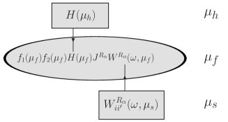
Figure 9: Sketch of the resummation of soft gluon corrections using renormalization group equations. Figure from [106].

Away from the production threshold large soft-gluon logarithms can appear in various other kinematic regions. When the relative velocity of the heavy particles is not small, Coulomb effects are not enhanced, and factorization takes the more standard form $H\cdot W$ without the $J$ function. However, the hard and soft functions now depend on the kinematic invariants of the general $2\to 2$ scattering process, as do the anomalous dimensions relevant to resummation. The soft function is no longer diagonal. Near threshold, interactions that change the colour-state of the heavy-particle pair appear only at the level of $\mathcal{O}(\beta^{2})$ ($\mathcal{O}(\beta)$) corrections to the total cross section (amplitude). Some of these effects are discussed in [106], but no calculation of $\mathcal{O}(\beta^{2})$ corrections in non-relativistic perturbation theory has so far been performed for hadronic processes.

4.1.2 Resummation

In the present framework the resummation of “Coulomb singularities” $(\alpha_{s}/\beta)^{n}$ is automatic in the $J$ function. The logarithms $(\alpha_{s}\ln^{2}\beta\,)^{n}$ are summed by solving the renormalization group equations to evolve the hard functions $H$ from the scale $\mu_{h}\sim M$, and the soft functions $W$ from the scale $\mu_{s}\sim M\beta^{2}$ to a common scale $\mu_{f}$, chosen to be the factorization scale of the parton distributions, as illustrated in Figure 9.

For the systematics of the combined resummations of the two types of corrections we count both $\alpha_{s}\ln\beta$ and $\alpha_{s}/\beta$ as quantities of order one and introduce a parametric representation of the expansion of the cross section of the form

The resummed cross section at LL accuracy includes all terms of order $1/\beta^{\,k}\times\alpha_{s}^{n+k}\ln^{2n}\beta$ relative to the Born cross section near threshold. Next-to-leading summation includes in addition all terms of order $\alpha_{s}\ln\beta;\,\alpha_{s}^{2}\{1/\beta\times\ln\beta,\ln^{3}\beta\};\ldots$, while furthermore all terms $\alpha_{s};\,\alpha_{s}^{2}\{1/\beta,\ln^{2,1}\beta\};\ldots$ are included in the NNLL approximation. With this counting, the formalism described above is limited to NNLL, since $\mathcal{O}(\beta^{2})$ terms are required beyond this order. A caveat applying to current NNLL treatments should be mentioned. Higher-order non-relativistic potentials cause ultraviolet singularities in the Coulomb function $J$, which cancel with the hard functions, and cause non-relativistic logarithms beginning with $\alpha_{s}^{2}\ln\beta$ at NNLL order. Present NNLL results (as described below) sum soft logarithms to all orders by evolution of the soft function, but include the non-relativistic logarithms only at fixed order $\alpha_{s}^{2}\ln\beta$.

The renormalization group equations and the formula for the resummed cross section are very similar to those derived for Drell-Yan production within the SCET framework [114, 115, 116], with the $HH^{\prime}$ pair in representation $R_{\alpha}$ replacing the colour-singlet Drell-Yan pair or electroweak gauge boson. The resummed partonic cross section then reads [105, 106]

and

$$\tilde{s}^{R_{\alpha}}_{i}(\rho,\mu)=\int_{0_{-}}^{\infty}d\omega e^{-s\omega}\,W_{i}^{R_{\alpha}}(\omega,\mu)$$ (60)

denotes the Laplace-transform of the $\overline{{\rm MS}}$-renormalized soft function with respect to $s=1/(e^{\gamma_{E}}\mu e^{\rho/2})$. The sum over the final-state representations $R_{\alpha}$ in the factorization formula (LABEL:eq:fact) has disappeared in the colour basis (54), since there is a unique final-state representation for each term in the sum over $i$. The resummed partonic cross section is then matched to the fixed-order cross section at the highest available order (NNLO for top quarks, NLO for supersymmetric particles), and integrated with the parton luminosity. The presence of the Coulomb functions introduces some subtleties in the convolution with the parton densities, which are discussed in [117].

For the definitions of the quantities appearing in (LABEL:eq:fact-resum), (LABEL:eq:def-u) we refer to [106], and mention only briefly the necessary ingredients for NNLL resummation. The hard functions are process-specific and must be obtained from the one-loop $2\to 2$ production cross sections directly at threshold, separated into irreducible colour (and if necessary, spin) representations. The soft function is also needed at one-loop, and has been computed for arbitrary colour representations in [105]. The single-particle and cusp anomalous dimension must be used at the two-loop and three-loop order, respectively, and are the same as for the Drell-Yan process. The only new anomalous dimension is the anomalous dimension $\gamma_{H,s}^{R_{\alpha}}$ for the soft function (56). In [105] the required expression has been related to the constant coefficient in the anomalous dimension of the heavy-heavy current in heavy-quark effective theory in the limit where the cusp angle goes to infinity. At the two-loop order relevant to NNLL resummation, the soft anomalous dimension exhibits Casimir scaling, $\gamma_{H,s}^{R_{\alpha}}=C_{R_{\alpha}}\gamma_{H,s}$. From the expression for the two-loop anomalous dimension of the heavy-heavy current [118, 119], one extracts

$$\gamma_{H,s}^{(1)}=-C_{A}\left(\frac{98}{9}-\frac{2\pi^{2}}{3}+4\zeta_{3}\right)+\frac{40}{9}T_{F}n_{f}$$ (61)

for the coefficient of $(\alpha_{s}/(4\pi))^{2}$. This result was confirmed by an explicit, independent calculation [120].

4.2 Top-pair invariant mass distribution near threshold

A Coulomb enhancement of the cross section for the production of top-quark pairs close to threshold, which has been discussed in Section 3 in the context of $e^{+}e^{-}$ collisions, can also be observed at hadron colliders, since it is possible to produce the top quarks in the colour-singlet state. Indeed, at LHC, the cross section close to threshold in dominated by the process $gg\to t\bar{t}$ where the top-quark pair is in the ${}^{1}S_{0}$ colour-singlet state. In contrast to a linear collider, where the physical observable is the total cross section as a function of energy, at the hadron collider one considers the invariant-mass distribution of the top-quark pairs.

The calculation of the cross section within the NRQCD framework contains as building blocks the hard production cross section for a top-quark pair at threshold [121, 122] and the non-relativistic Green function governing the dynamics of the would-be toponium bound-state. In [121] the NLO formulae were derived for quark or gluon initial states and a quarkonium in a $\mbox{J}^{\mbox{\scriptsize PC}}=0^{-+}$ colour-singlet state, plus possibly a parton. The general case, with the heavy quark system $(Q\bar{Q})$ in S-wave singlet/triplet spin state, and colour-singlet/octet configuration is given in [122], together with the corresponding results for P-waves. The results of [121, 122] were presented for stable bound states. For wide resonances it is convenient to describe the bound-state dynamics through a Green function.

NLO calculations have been performed in [111, 112], where slightly different approaches have been applied. Whereas in [112] the matching has been performed in the strict threshold limit where the partonic centre-of-mass energy $\hat{s}$ approaches twice the top-quark mass, the complete dependence on $\hat{s}$ as given in [121, 122] is included in [111]. Thus, formally, the result of [112] is only valid for top-quark production where the velocity of both quarks is small. In the approach of [111] on the other hand, the relative velocity still has to be small but the combined top-antitop quark system can move with high velocity. Furthermore, Ref. [111] includes all NLO subprocesses, i.e. also those which appear for the first time in ${\cal O}(\alpha_{s}^{3})$ and performs a soft gluon resummation at the NLL order using the Mellin-space approach.

In Figure 10 the invariant-mass distributions for LHC with $\sqrt{s}=14$ TeV centre-of-mass energy is shown for the sum of all contributing channels and separately for the colour-octet and colour-singlet contribution. The width of the bands is obtained from varying renormalization and factorization scales in the hard cross section as described above. The additional uncertainty from the Green function, which is estimated to about 20% for the singlet and below 5% for the octet case [111], is not included.

As expected, for invariant mass $M<2m_{t}$ the production of $t{\bar{t}}$ pairs is dominated by the singlet contribution. However, for $M>2m_{t}$ one observes a strong rise of the octet contributions, in particular of the gluon-induced subprocess, which for $M\;\hbox to0.0pt{\lower 3.5pt\hbox{$\mathchar 0\relax\sim$}\hss}\raise 1.0pt\hbox{$>$}\;2m_{t}+5$ GeV becomes even larger than the corresponding singlet contribution. For the colour-octet case the scale dependence of the hard scattering amounts to $\pm 7\%$. Considering the threshold behaviour as shown in Figure 10 it is clear that the location of the threshold is entirely governed by the behaviour of the colour-singlet (S-wave) contribution. Thus, as a matter of principle, determining the location of this step experimentally would allow for a top-quark mass measurement, which is conceptually very different from the one based on the reconstruction of a (coloured) single quark in the decay chain $t\to Wb$. In fact, much of the detailed investigations of $t\bar{t}$ threshold production at a linear collider were performed for this situation by establishing the relation between the location of the colour singlet top-antitop resonance and the top-quark $\overline{\mbox{MS}}$-mass.

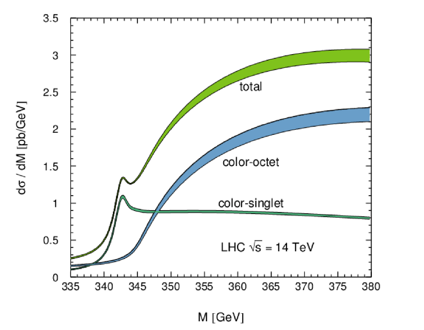
Figure 10: Invariant-mass distribution for top-quark pair production. The width of the bands reflect the scale dependence of the hard scattering parts. Figure from [111].

Considering the threshold region (say up to $M_{t\bar{t}}=350\leavevmode\nobreak\ {\rm GeV}$) separately, an integrated cross section of 15 pb is obtained, which should be compared to 5 pb as derived from the NLO predictions using a stable top quark and neglecting the binding Coulomb-force correction. Within this relatively narrow region the enhancement amounts to roughly a factor three and a significant shift of the threshold. Compared to the total cross section for $t\bar{t}$ production of about 900 pb, the increase is relatively small, about 1%. However, in view of the present and future experimental precision these effects should not be ignored.

4.3 Total top pair production cross section

The ability of LHC to produce top-quark pairs in large numbers has triggered a large amount of theoretical work devoted to improving the accuracy of the prediction of the total cross section. The first results referred to approximate NNLO (“NNLO_app”) calculations that aimed at including the singular terms in the partonic cross section as $\beta\to 0$ [123, 124, 125, 126]. Soft-gluon resummation of the total cross section with NNLL accuracy was completed in [117, 127] with two independent calculations, one done in the joint soft-Coulomb resummation approach described above, the other in the Mellin-space soft-gluon resummation formalism. In yet another approach the total cross section is computed from NNLL-resummed or approximated NNLO calculations of certain differential distributions [128, 129, 130].

It should be noted that threshold resummation for the top-pair inclusive cross section does not have a clear parametric justification. In order to obtain the total hadronic cross section, the partonic cross section is convoluted with the parton distribution functions. Both at Tevatron and LHC, the top-antitop invariant-mass distribution peaks at about $400\,$GeV, which corresponds (in the absence of radiation) to $\beta\approx 0.5$. The convolution of the partonic cross section with the parton luminosity is therefore dominated by the region $\beta>0.3$, where the threshold approximation is no longer valid. Nevertheless, one often finds that the threshold expansion provides a reasonable approximation even outside its domain of validity. At the very least, the approximation is better than the one not using this piece of information.

Much of the ambiguity in resummed calculations has been removed through the fixed-order NNLO calculation [131, 132]. The present state-of-the-art prediction therefore consists of NNLL resummation matched to the full NNLO result, and is available in the programs Topixs [133] (based on [117]) and top++ [134] (based on [127]). Topixs includes soft and Coulomb resummation and is therefore technically the most complete theoretical prediction. In particular, it includes the bound-state effects in the threshold region discussed in the previous subsection. However, the effect of Coulomb resummation beyond the terms already included in the fixed-order NNLO result is rather small for the total cross section.

$\sigma_{t\bar{t}}$[pb]	Tevatron	LHC ($\sqrt{s}=$7 TeV)	LHC ($\sqrt{s}=$8 TeV)
NLO	$6.68^{+0.36+0.23}_{-0.75-0.22}$	$158.1^{+19.5+6.8}_{-21.2-6.2}$	$226.2^{+27.8+9.2}_{-29.7-8.3}$
NNLOapp	$7.06^{+0.26+0.29}_{-0.34-0.24}$	$161.1^{+12.3+7.3}_{-11.9-6.7}$	$230.0^{+16.7+9.7}_{-15.7-9.0}$
NNLO	$7.01^{+0.27+0.29}_{-0.37-0.24}$	$167.1^{+\phantom{0}6.7+7.7}_{-10.7-7.1}$	$239.1^{+9.2+10.4}_{-14.8-9.6}$
NNLL	$7.15^{+0.24+0.30}_{-0.10-0.25}$	$168.5^{+\phantom{0}6.3+7.7}_{-\phantom{0}7.5-7.2}$	$241.0^{+8.7+10.5}_{-11.1-9.7}$

Table 1: Top-quark pair production cross section at Tevatron and LHC for $m_{t}=173.3\,$GeV, $\alpha_{s}(M_{Z})=0.1171\pm 0.0014$, (N)NLO MSTW08 PDFs [135]. The first error represents to theoretical uncertainty from independent soft/hard/Coulomb scale variations and resummation ambiguities in the partonic cross section, the second PDF+$\alpha_{s}$ at 68% CL.

In Table 1 we summarize successive approximations to the top-quark pair production cross section at Tevatron and LHC from NLO to NNLL, where NNLL means resummed matched to full NNLO, generated with Topixs 2.0. We note that in production at the Tevatron, which is dominated by the quark-antiquark initial state, the resummation/NNLO effect is significant ($+8\%$, NNLL vs. NLO in the table), and the threshold approximation to the full result worked well (NNLO vs. NNLO_app). On the other hand, in gluon-gluon initiated production at the LHC, resummation is a small correction ($+1\%$) and underestimates the full NNLO correction ($+4\%$). However, in both cases, resummation without the full NNLO correction already leads to a significant reduction of the theoretical uncertainty ($8\%\to 3\%$ at Tevatron, $13\%\to 4.5\%$ at LHC, excluding the PDF + $\alpha_{s}$ error), while still including the full NNLO+NNLL result in the uncertainty estimate.

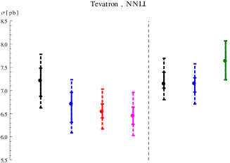
Tevatron, NNLL

      $\sigma[pb]$

Figure 11: Top-pair production cross section calculations with NNLL accuracy in $p\bar{p}$ collisions at $\sqrt{s}=1.96\,$TeV (Tevatron). To the left of the dashed line: NNLO_app + NNLL results. Black: Beneke et al. [117] and Topixs 1.0 ($m_{t}=173.3$ GeV); Blue: Cacciari et al. [127] ($m_{t}=173.3$ GeV) Red: Ahrens et al. [129] (1PI, $m_{t}=173.1$ GeV) Magenta: Ahrens et al. [129] (PIM, $m_{t}=173.1$ GeV) To the right of the dashed line: full NNLO + NNLL results. Black: Update of Beneke et al. [133] and Topixs 2.0 ($m_{t}=173.3$ GeV) Blue: Czakon et al. [132] and top++2.0 ($m_{t}=173.3$ GeV) Darkgreen: CDF/D0 combined measurement quoted from CMS/ATLAS-CONF-2012-149. Error bars: inner solid – theory uncertainty of the partonic cross section excluding $\alpha_{s}$, outer dashed – PDF (+$\alpha_{s}$) added. PDF set: MSTW2008 NNLO with $\alpha_{s}(M_{Z})=0.1171\pm 0.0014$.

Figure 11 summarizes the results for the total top-pair cross section at the Tevatron from different theoretical calculations. By comparing the black and blue bars to the left and right of the vertical dashed line, we observe that the predictions from joint soft-Coulomb resummation (first bar [black], [133]) and the Mellin-space approach (second bar [blue], [132]) are in very good agreement, once the full NNLO result is included and resolves some of the resummation ambiguities (in favour of the former). The NNLO+NNLL computations are in good agreement with the measurement for the adopted top-quark pole mass $m_{t}=173.3$ GeV, while the NLO result would underestimate the measurement significantly (compare Table 1).

The top-quark pair cross section has become a precisely predicted and measured quantity, which depends essentially only on the fundamental parameters $m_{t}$ and $\alpha_{s}$, and the parton distributions. Assuming standard physics the measurement constrains these parameters. The possibility to determine the top-quark mass in a theoretically clean way, though less precisely than from reconstruction of top decay products, has been explored, for instance, in [117, 133, 136, 137]. The determination of the strong coupling has been considered in [138]. The impact of the top-quark cross section at LHC on the gluon distribution in the proton has been investigated first in [133], and in more detail in [139] within the NNPDF framework. See also [140].

4.4 Pair production of supersymmetric particles

The search for the partners of the SM particles predicted by supersymmetric extensions of the SM is an integral part of the LHC physics programme. Present exclusions already imply that the masses of the strongly interacting squarks and gluinos are most likely in the TeV range. For such heavy particles, threshold resummation is expected to be important, and, contrary to the case of top quarks, even parametrically relevant, as a larger fraction is produced close to the partonic threshold due to the fall-off of the parton distributions at large momentum fraction.

The study of soft-gluon resummation for pair production of supersymmetric particles was initiated by [113, 141]. The NLL analysis of the squark-antisquark, squark-squark, (anti) squark-gluino and gluino-gluino final states [142] finds significant corrections of several 10% beyond the fixed-order NLO calculation, especially for the gluino-gluino final state, which involves the largest colour charges. Note, that NLO corrections to gluino bound-state production has been considered in [143, 144] and gluino pair production close to threshold is presented in [145].

The resummation formalism for soft and Coulomb gluons was in fact first used to predict squark-antisquark production [106] in the NLL approximation as defined in (LABEL:eq:syst) and then extended to all superparticle pair final states in [146], which also generalized the factorization formula to a particular case of P-wave production relevant to stop-antistop production. A scenario with superparticles with substantial decay widths (for instance, gluinos decaying further into squarks and quarks) was also investigated [147], which adds the complication of unstable-particle effects and non-resonant production.

Different from top-pair production, the summation of Coulomb effects is important for some final states, which becomes apparent in large differences between the NLL results of [142] and [106, 146]. The size of the resummation effects can be quantified by

$$K_{\rm NLL}=\frac{\sigma_{\rm NLL,\,matched}}{\sigma_{\rm NLO}},$$ (62)

where $\sigma_{\rm NLL,\,matched}$ is the resummed result, properly matched to the full NLO calculation. The NLL soft- and Coulomb-resummed result is shown as solid line in Figure 12, the one without Coulomb summation is the dashed NLL_s+h line. In squark-antisquark production (upper panel), for large squark masses, the resummation effect is more than a factor of four larger in the former treatment, which highlights the effect of Coulomb attraction. No such effect is observed in the squark-squark production process (middle panel), due to a cancellation between the numerically dominant, repulsive colour-sextet channel for same-flavour squark production, and an attractive colour-triplet channel in different-flavour squark production [146]. Gluino-gluino production lies in between these extreme cases, but shows the largest resummation effects as already mentioned above. Figure 12 also demonstrates that bound-state production (or rather, the resonant enhancement in and below the nominal threshold region) provides a significant further enhancement of the total cross section, given by the difference between the dot-dashed and solid lines.

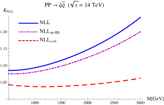
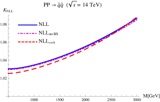
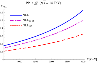
Figure 12: NLL K-factor for squark-antisquark (top), squark-squark (middle), and gluino-gluino (bottom) production at LHC with $\sqrt{s}=14\,$TeV. The plots show $K_{\rm NLL}$ as a function of $M=m_{\tilde{g}}=m_{\tilde{q}}$ for different NLL approximations: NLL (solid blue), NLL_noBS (bound-state contributions excluded, dot-dashed purple) and NLL_s+h (dashed red). See the text for explanation. Figure from [146].

The main difference between [142] and [106, 146] can be traced to the soft and Coulomb interference term at NNLO, which is already included in NLL soft-Coulomb resummation, but not in NLL soft-gluon resummation alone. The difference should therefore be reduced, when soft-gluon without Coulomb resummation is extended to NNLL as has indeed been confirmed by [148]. NNLL results in both frameworks have meanwhile been presented [149, 150] for all final states, and an additional result is available for gluino pairs [151].

5 Sommerfeld enhancement of dark matter pair annihilation

In this last section we turn to a potentially important non-relativistic effect in the pair annihilation of dark matter (DM) particles. While the nature and origin of dark matter are still unknown it is intriguing that the observed abundance can be explained rather naturally as thermal relic of a TeV scale particle with weak interaction strength. The relic density is determined by the total annihilation cross section, $\langle\sigma v\rangle$, averaged over the velocity distribution of the particles. Since the abundance froze out when the temperature of the Universe was about $M_{\chi}/25$, where $M_{\chi}$ is the DM particle mass, the typical velocities $v\sim 0.2$ are non-relativistic. When DM particles annihilate in the present Universe, potentially revealing themselves in cosmic ray signatures, the typical velocities are $v\sim 10^{-3}$, and the annihilation occurs even deeper in the non-relativistic regime.

For heavy, weakly interacting, TeV-scale dark matter the exchange of the electroweak gauge (and Higgs) bosons between the slowly moving DM particles generates a Yukawa potential, which leads to an enhancement of ladder diagrams. Unlike the case of the long-range Coulomb potential due to gluon or photon exchange discussed up to now, the enhancement does not increase as $\alpha_{\rm EW}/v$ at very small velocities, but is cut off at $\alpha_{\rm EW}M_{\chi}/M_{W}$ by the mass of the mediator particle. Nevertheless, additional particle exchange is not suppressed by the size of the electroweak coupling $\alpha_{\rm EW}$ when the DM mass is much larger than the mediator mass. This so-called Sommerfeld effect can exceed the lowest-order annihilation cross section by orders of magnitude. The Yukawa potential has only a finite number of bound states of order $\mathcal{O}(\alpha_{\rm EW}M_{\chi}/M_{W})$. When the dark matter mass is varied, resonant enhancements of the DM pair scattering wave-functions occur whenever a bound state approaches the threshold, which can yield pronounced Sommerfeld enhancements stronger than in the Coulomb case.

The relevance of the Sommerfeld effect was first pointed out for (wino- or higgsino-like) neutralino DM annihilation into two photons [152], and subsequently for relic-density calculations [153], although it was not until 2008, when an anomalous positron excess was measured by PAMELA, that Sommerfeld enhanced DM models attracted more attention as a mechanism to boost the DM annihilation rates [154]. We note that for heavy dark matter with mass far above the electroweak scale, the mass splittings between the states of the DM electroweak multiplet are naturally in the GeV or sub-GeV range. At freeze-out a multitude of co-annihilation processes, including charged states are still active, and Sommerfeld enhancements are generic. This occurs in particular in the minimal supersymmetric standard model (MSSM). Sommerfeld enhancements in cosmic ray signatures and in the thermal relic abundance have therefore been discussed extensively for relevant MSSM scenarios with neutralino DM [155, 156, 157, 158, 159, 160, 161], but also for generic multi-state dark matter models [162, 163, 164].

In the following we summarize the work of [165, 166, 167, 168], which aims at improving the calculation of the dark-matter annihilation cross section and relic abundance by including the Sommerfeld radiative corrections in the general MSSM, beyond the previously considered wino- and Higgsino-limit, where the neutralino can be an arbitrary admixture of the electroweak wino, Higgsino and bino states. As in previous sections a non-relativistic effective theory (of the MSSM) is constructed to separate the short-distance annihilation process from the long-distance Sommerfeld effect, which is encoded in the matrix elements of local four-fermion operators. The approach is very similar to the NRQCD treatment of quarkonium annihilation [5], except that we deal with scattering states of several species of particles interacting through the electroweak Yukawa force.

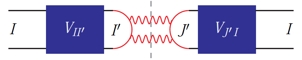
Figure 13: Graphical representation of the $I\to I$ forward-amplitude. The square stand for the action of the potential (the sum of ladder diagram) that scatters $I$ into another state $I^{\prime}$ ($J^{\prime}$ in the conjugated amplitude), which then annihilates into a final state of Standard Model particles (and MSSM Higgs bosons, if kinematically allowed). [Figure: courtesy C. Hellmann]

The presence of several particle species $\chi_{i}$ entails many complications. Since electroweak gauge boson exchange may change the two-particle state (for instance, scatter a neutralino pair into a pair of oppositely charged, nearly degenerate, charginos), the short-distance annihilation process is described by a matrix in the space of two-particle states, which is not diagonal. The off-diagonal terms cannot be obtained from the tree-level cross sections computed by numerical programs. The non-relativistic expansion of the short-distance annihilation cross section is therefore computed analytically rather than numerically, which is also necessary to separate S- and P-wave, and spin-0 and spin-1 annihilation contributions, which receive different Sommerfeld enhancement factors. The large number of final and initial states in the MSSM imply that several thousand processes have to be computed. The long-distance part of the problem then involves the solution of a matrix-valued Schrödinger equation in the space of $\chi_{i}\chi_{j}$ two-particle states. The existence of kinematically closed channels leads to numerical instabilities that requires a new method to determine the scattering wave functions at the origin relevant to the Sommerfeld enhancement. These issues together with a few results are summarized below. For many further relevant details, we refer to [165, 166, 167, 168].

5.1 Construction of the annihilation rates

The process we are interested in is shown schematically in Figure 13 and is described by the non-relativistic MSSM Lagrangian

$$\mathcal{L}^{\rm NRMSSM}=\mathcal{L}_{\rm kin}+\mathcal{L}_{\rm pot}+\delta\mathcal{L}_{\rm ann}+\dots\,$$ (63)

$\mathcal{L}_{\rm kin}$ contains the bilinear terms in the two-component spinor fields $\xi_{i}$ and $\psi_{j}=\eta_{j},\zeta_{j}$ that represent the $n_{0}\leq 4$ non-relativistic neutralinos ($\chi^{0}_{i}$) and $n_{+}\leq 2$ charginos ($\chi^{-}_{j}$ and $\chi^{+}_{j}$), respectively. The entire treatment is restricted to the leading-order terms in the velocity expansion in the long-distance part, hence $\mathcal{L}_{\rm kin}$ is simply given by

$$\mathcal{L}_{\rm kin} \!\!=\!\! \sum\limits_{i=1}^{n_{0}}\xi^{\dagger}_{i}\left(i\partial_{t}-(m_{i}-m_{{\rm LSP}})+\frac{\vec{\partial}^{\,2}}{2m_{\mathrm{LSP}}}\right)\xi_{i}\quad$$ (64)

$$+\sum_{\psi=\eta,\zeta}\sum\limits_{j=1}^{n_{+}}\psi^{\dagger}_{j}\left(i\partial_{t}-(m_{j}-m_{{\rm LSP}})+\frac{\vec{\partial}^{\,2}}{2m_{\mathrm{LSP}}}\right)\psi_{j}.\qquad$$

The non-relativistic energy is measured relative to the mass $m_{{\rm LSP}}$ of the lightest neutralino state. To have a consistent power-counting, the mass differences $(m_{i}-m_{{\rm LSP}})$ must formally be considered of order $m_{\rm LSP}v^{2}$.

The short-distance annihilation of the chargino and neutralino pairs into SM and light Higgs final states is reproduced in the effective field theory by local four-fermion operators. The leading-order contributions to $\delta\mathcal{L}_{\rm ann}$ are given by dimension-6 four-fermion operators, that describe leading-order S-wave neutralino and chargino scattering processes $\chi_{e_{1}}\chi_{e_{2}}\to\chi_{e_{4}}\chi_{e_{3}}$. They read

where $f^{\chi\chi\to\chi\chi}_{\{e_{1}e_{2}\}\{e_{4}e_{3}\}}\left({}^{2S+1}L_{J}\right)$ are the corresponding short-distance coefficients. The explicit form of the dimension-6 S-wave operators with spin $S=0,1$ is

$$\mathcal{O}^{\chi\chi\to\chi\chi}_{\{e_{4}e_{3}\}\{e_{2}e_{1}\}}\left({}^{1}S_{0}\right)\, = \ \chi^{\dagger}_{e_{4}}\chi^{c}_{e_{3}}\ \chi^{c\dagger}_{e_{2}}\chi_{e_{1}}\ ,$$ (66)

$$\mathcal{O}^{\chi\chi\to\chi\chi}_{\{e_{4}e_{3}\}\{e_{2}e_{1}\}}\left({}^{3}S_{1}\right)\, = \ \chi^{\dagger}_{e_{4}}\sigma^{i}\chi^{c}_{e_{3}}\ \chi^{c\dagger}_{e_{2}}\sigma^{i}\chi_{e_{1}}\ .$$ (67)

The first sum in (LABEL:eq:deltaL4fermion) is taken over all neutralino and chargino forward-scattering reactions $\chi_{e_{1}}\chi_{e_{2}}\to\chi_{e_{4}}\chi_{e_{3}}$, including redundant ones where the particle species at the first and second and/or third and fourth position are interchanged. Thus in the sector of two-particle states with electric charge $Q$, $f^{\chi\chi\to\chi\chi}_{\{e_{1}e_{2}\}\{e_{4}e_{3}\}}$ is a square matrix of dimension $N_{Q}=(N_{0},N_{1},N_{2})=(24,16,4)$. In order to reproduce the short-distance tree-level annihilation cross section with $\mathcal{O}(v^{2})$ accuracy, we add dimension-8 operators with two derivatives accounting for P-wave and corrections to S-wave annihilation, but also operators proportional to the mass differences $\delta m=(m_{e_{4}}-m_{e_{1}})/2$, $\delta\overline{m}=(m_{e_{3}}-m_{e_{2}})/2$. Of course, the latter have non-vanishing coefficients only for the off-diagonal elements of forward amplitude.

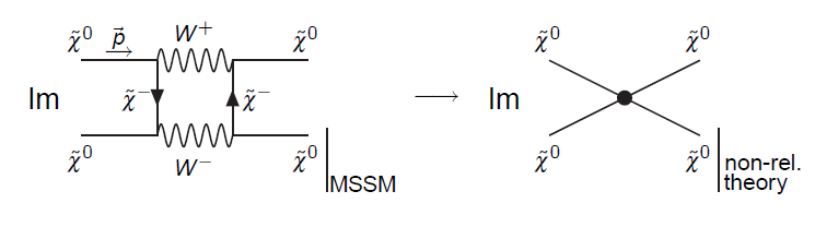
Figure 14: Matching of the imaginary part of the forward amplitude. [Figure: courtesy C. Hellmann]

The short-distance coefficients of all these operators are determined by expanding the MSSM amplitudes for the process $\chi_{e1}\chi_{e_{2}}\to X\to\chi_{e_{4}}\chi_{e_{3}}$ with SM and light Higgs intermediate states in the relative momenta $\vec{p}$, $\vec{p}^{\,\prime}$ and mass differences $\delta m$, $\delta\overline{m}$, and matching them to the tree-level matrix element of the four-fermion operators for the same incoming and outgoing states to $\mathcal{O}(v^{2})$, as illustrated in Figure 14. For the computation of the neutralino and chargino inclusive annihilation rates, only the absorptive part of the short-distance coefficients are required according to the optical theorem. At tree-level, it is also possible to define the rates to exclusive final states (relevant to indirect detection of DM) in this way. We note that the matching is performed for on-shell scattering, which implies that $\vec{p}$ and $\vec{p}^{\,\prime}$ are different for the off-diagonal scatterings. Energy conservation implies that

$$\frac{\vec{p}^{\,2}}{2\mu} = \sqrt{s}-M+(\,\delta m+\delta\overline{m}\,)+\dots\ ,$$ (68)

$$\frac{\vec{p}^{\,\prime\,2}}{2\mu} = \sqrt{s}-M-(\,\delta m+\delta\overline{m}\,)+\dots,$$ (69)

where $\sqrt{s}$ is the centre-of mass energy of the scattering, $M=(\sum_{i=1}^{4}m_{e_{i}})/2$, $m=(m_{e_{1}}+m_{e_{4}})/2$, $\overline{m}=(m_{e_{2}}+m_{e_{3}})/2$, and $\mu=m\overline{m}/M$. The non-relativistic expansion is strictly valid, when $\sqrt{s}-M$, $\delta m$ and $\delta\overline{m}$ are of order $M_{\chi}v^{2}$.

The actual calculation is complicated by the presence of many final states and interactions in the MSSM. Moreover, for reasons discussed in [165], the calculation is most easily done in ‘t Hooft-Feynman gauge, which, however, adds a large number of unphysical final states containing pseudo-Goldstone Higgs and ghost particles. The calculation of all S-wave annihilation rates is presented in [165], and the coefficients of the $\mathcal{O}(v^{2})$ terms in [166].

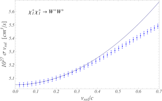
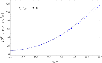
Figure 15: Numerical comparison of the non-relativistic approximation (solid lines) to the tree-level annihilation cross-section times relative velocity, $\sigma\,v_{\rm rel}$, for $\chi^{+}_{1}\chi^{+}_{1}\to W^{+}W^{+}$ (upper figure) and $\chi^{+}_{1}\chi^{-}_{2}\to H^{+}H^{-}$ (lower figure) with the corresponding unexpanded annihilation cross section produced with MadGraph [169]. The second process is dominated by P-wave annihilation. $v_{\rm rel}$ is given by $v_{\rm rel}=|\vec{v}_{e_{1}}-\vec{v}_{e_{2}}|$ for the $\chi_{e_{1}}\chi_{e_{2}}\to X_{A}X_{B}$ process. The underlying MSSM spectrum is a wino-like neutralino LSP scenario, generated with the spectrum calculator SuSpect [170]. The masses of the $\chi^{0}_{1}$ and $\chi^{+}_{1}$ are given by $m_{\chi^{0}_{1}}=2748.92\,\mbox{GeV}$, $m_{\chi^{+}_{1}}=2749.13\,\mbox{GeV}$, and $m_{\chi^{-}_{2}}=3073.31\,\mbox{GeV}$. The mass of the Higgs particles $H^{\pm}$ takes the value $m_{H^{\pm}}=167.29\,\mbox{GeV}$. Figure from [165].

The non-relativistic expansion to $\mathcal{O}(v^{2})$ is usually a very good approximation. For the diagonal annihilation rates, the result from the above calculation can be compared to the unexpanded tree-level cross section. A comparison for two cases is shown in Figure 15. Good agreement is found up to relative velocities of about 0.5, which is sufficient for all practical purposes. The analytic expressions from [165, 166] cover all relevant processes, when only neutralino and chargino (co-) annihilation processes are relevant. MSSM scenarios with sfermion-neutralino co-annihilation are presently not covered, neither are resonant annihilation models, since in this case the annihilation process is no-longer short-distance, and cannot be expanded in the velocity.

5.2 Computation of the Sommerfeld enhancement

Once the short-distance coefficients are at hand, the Sommerfeld-enhancement is computed from the matrix elements of four-fermion operators such as (66), (67). The first step consists in deriving the potentials in the expression

which contains spin-independent and spin-dependent terms. The indices $\alpha_{i}$ are contracted with the (unwritten) spin indices of the field operators in (LABEL:eq:pot), and the total spin operator $\vec{S}$ is $\vec{S}_{\alpha_{4}\alpha_{1},\alpha_{3}\alpha_{2}}=\vec{\sigma}_{\alpha_{4}\alpha_{1}}/2\,\delta_{\alpha_{3}\alpha_{2}}+\delta_{\alpha_{4}\alpha_{1}}\vec{\sigma}_{\alpha_{3}\alpha_{1}}/2$. Since the total spin is not changed at this order, the two-particle states $\chi_{e_{1}}\chi_{e_{2}}$ and $\chi_{e_{4}}\chi_{e_{3}}$ undergoing potential interactions can be decomposed into ${}^{2S+1}L_{J}$ partial-wave states with defined spin $S=0,1$, and the Sommerfeld factors can be determined separately for each spin. The MSSM neutralino-chargino potentials are given in [167].

The resummation of ladder diagrams carrying the Sommerfeld enhancement is achieved by including the interaction (LABEL:eq:pot) into the unperturbed Lagrangian. The task is then to evaluate the matrix elements of the annihilation operators in this theory. For the general treatment we refer to [167] and consider here the example of the ${}^{1}S_{0}$ operator (66). Its matrix element can be parametrized in the form

where (in general) $\psi^{(L,S)}_{e_{1}e_{2},\,ij}$ is the $\chi_{e_{1}}\chi_{e_{2}}$-component of the scattering wave function for an incoming $\chi_{i}\chi_{j}$ state with centre-of-mass energy $\sqrt{s}$, orbital quantum number $L$ and total spin $S$, evaluated for zero relative distance and normalized to the free scattering solution. In the absence of potential interactions, the tree-level matrix element of the four-fermion operators is obtained by replacing $\psi^{(L,S)}_{e_{a}e_{b},\,ij}\to\delta_{e_{a}i}\,\delta_{e_{b}j}$. It is convenient to introduce a notation where a single index refers to a two-particle state (for instance, $e={e_{1}e_{2}},i={ij}$) rather than two indices for the individual particle species that make up this state. The Sommerfeld factor is defined as the annihilation cross section including the potential interaction relative to the tree cross section. For a given partial-wave contribution to the annihilation cross section, it is defined as

$$S_{i}[\hat{f}(^{2S+1}L_{J})]=\frac{\left[\psi^{(L,S)}_{e^{\prime}i}\right]^{*}\hat{f}_{ee^{\prime}}(^{2S+1}L_{J})\,\psi^{(L,S)}_{ei}}{\hat{f}_{ii}(^{2S+1}L_{J})|_{\rm LO}}.$$ (73)

Here $\hat{f}_{ee^{\prime}}$ is related to the absorptive part of $f^{\chi\chi\to\chi\chi}_{ee^{\prime}}$. A sum over all two-particle states $e$, $e^{\prime}$ is implicit in (73).

The annihilation cross section including the Sommerfeld corrections is constructed by multiplying each spin and partial-wave component by its respective Sommerfeld factor (73). The tree-level cross section expanded to $\mathcal{O}(v^{2})$ is recovered by setting $S_{i}[\hat{f}(^{2S+1}L_{J})]\to 1$. Defining $\vec{p}_{i}^{\,2}=2\mu_{i}\,(\!\sqrt{s}-M_{i})+\mathcal{O}(\vec{p}_{i}^{\,4})$, the relative momentum squared of the two annihilating neutralinos, and $M_{i}$ and $\mu_{i}$, the total and reduced mass, respectively, of the two-particle system, the master formula for the cross section takes the form

The precise definition of the annihilation matrices appearing in this equation is given in [167].

It is well-known that the matrix elements of four-fermion operators can be expressed (at this order in the non-relativistic expansion) in terms of wave functions at the origin. In the present case $\psi^{(0,S)}_{ei}=[\psi_{E}(0)]_{ei}^{*}$ with $\psi_{E}(\vec{r}\,)$ the matrix-valued solution of the Schrödinger equation

$$\left(\left[-\frac{\vec{\nabla}^{\,2}}{m_{\rm LSP}}-E\right]\delta^{ab}+V^{ab}(r)\right)[\psi_{E}(\vec{r}\,)]_{bi}=0.$$ (75)

Here $E=\sqrt{s}-2m_{\rm LSP}$ and

$$V^{ab}(r)=\hat{V}^{ab}(r)+\delta^{ab}\,\big{[}M_{a}-2m_{\rm LSP}\big{]}\,.$$ (76)

We also use the velocity variable $v$ defined by

$$E\equiv m_{\rm LSP}v^{2}\,.$$ (77)

The solution method proposed in [171] (and reviewed in [167] in the present notation) relates the Sommerfeld enhancement to the asymptotic behaviour of the radial partial-wave function $u(r)$ for certain boundary conditions at $r=0$. For the S-wave case, one finds

$$[\psi_{E}(0)]_{ei}^{*}=[U^{-1}(r_{\infty})]_{ei},$$ (78)

where $U$ is the matrix

$$U_{ab}(r_{\infty})=e^{ik_{a}r_{\infty}}\,\left([u^{\prime}(r_{\infty})]_{ab}-ik_{a}[u(r_{\infty})]_{ab}\right),\;$$ (79)

and $k_{a}^{2}=m_{\rm LSP}(E+i\epsilon-[M_{a}-2m_{\rm LSP}])$ for a two-particle state $a$ with mass $M_{a}$. The Schrödinger equation must be solved from $r=0$ to a value $r_{\infty}$ large enough such that $U_{ab}(r_{\infty})$ is close enough to its asymptotic value.

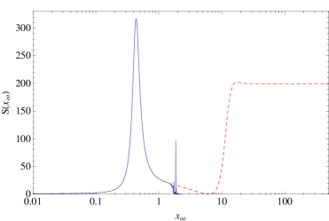
Figure 16: S-wave spin-0 Sommerfeld factor for $v=0.012$ in a wino-like model as described in the text. The light-grey (red) dashed curve shows $S(x_{\infty})$, when only the $\chi_{1}^{0}\chi_{1}^{0}$ and $\chi_{1}^{+}\chi_{1}^{-}$ two-particle states in the Schrödinger equation and the annihilation process are kept and the asymptotic regime is reached for $x_{\infty}>50$. The dark-grey (blue) solid curve shows the result when the $\chi_{1}^{0}\chi_{2}^{0}$ state is included. In this case, the evaluation fails for $x_{\infty}>2$ and no reliable result is obtained. Figure from [167].

The procedure described here works well, when all  $N$ states included in the multi-channel Schrödinger equation are degenerate to a high degree, but fails otherwise. This is illustrated in Figure 16, which shows the Sommerfeld factor for the $\chi_{1}^{0}\chi_{1}^{0}$ ${}^{1}S_{0}$ annihilation cross section as function of $x_{\infty}=m_{\rm LSP}v\,r_{\infty}$ for a MSSM parameter point where the lightest neutralino (LSP) is wino-like. The relevant masses are $m_{\rm LSP}=m_{\chi_{1}^{0}}=2749.4\,$GeV, $m_{\chi_{1}^{+}}=2749.61\,$GeV and $m_{\chi_{2}^{0}}=2950.25\,$GeV. The light-grey (red), dashed curve shows $S(x_{\infty})$ when only the two highly degenerate $\chi_{1}^{0}\chi_{1}^{0}$ and $\chi_{1}^{+}\chi_{1}^{-}$ two-particle states are included in the Schrödinger equation and the annihilation process. The velocity is chosen $v=0.012$, slightly below the threshold for the $\chi_{1}^{+}\chi_{1}^{-}$ state. After a rapid variation with a peak structure, the Sommerfeld factor reaches a plateau and for $x_{\infty}>50$ stays at the constant value $S(\infty)\approx 199.59$. When the $\chi_{1}^{0}\chi_{2}^{0}$ state is added to the problem, the Schrödinger system is extended to a $3\times 3$ matrix. Since the new state is $200\,$GeV heavier and moreover rather weakly coupled to the two lowest, nearly degenerate wino states, it should have little effect on the value of the Sommerfeld factor. However, now the numerical solution fails when $x_{\infty}$ is slightly larger than 1, as seen from the dark-grey (blue) solid curve in Figure 16, which drops to 0 after a few spikes. It is not possible to reach the plateau, where $S(x_{\infty})$ stabilizes.

The numerical instability originates from the presence of kinematically closed two-particle state channels, here the $\chi_{1}^{0}\chi_{2}^{0}$ state. The solution $[u(x)]_{bi}$ for the closed channel involves an exponentially growing component proportional to $e^{\kappa_{b}r}$ where $\kappa_{b}^{2}=m_{\rm LSP}(M_{b}-[2m_{\rm LSP}+m_{\rm LSP}v^{2}])$. The off-diagonal potentials $V^{ab}(r)$ couple the different channels and the open-channel solutions $[u_{l}(x)]_{ai}$ inherit the exponential growth from the closed channels. For the two-LSP $\chi_{1}^{0}\chi_{1}^{0}$ channel, exponential growth occurs when at least one of the included kinematically closed channels $b$ satisfies

$$M_{b}-[2m_{\rm LSP}+m_{\rm LSP}v^{2}]>\frac{M_{\rm EW}^{2}}{m_{\rm LSP}}\,.$$ (80)

Since typically $m_{\rm LSP}\gg M_{\rm EW}$ for the dark-matter scenarios of interest, this condition is easily satisfied unless all two-particle states included in the computation are degenerate within a few GeV or less. In consequence the formally linearly independent solutions $[u]_{ai}$ degenerate and the matrix $U_{ai}$ becomes ill-conditioned with exponentially growing entries in the rows corresponding to open channels $a$. The matrix inversion required for (78) can no longer be done in practice for $r_{\infty}$ large enough such that the asymptotic regime is reached, which causes the instability seen in Figure 16.

The solution to the problem provided in [167] is based on an adaptation of the modification of the variable-phase method for the Schrödinger problem [172]. The idea is to write the solution as a linear combination of the linearly independent Bessel function solutions $f_{a}(x)$, $g_{a}(x)$ of the free Schrödinger problem:

$$[u(x)]_{ai}=f_{a}(x)\alpha_{ai}(x)-g_{a}(x)\beta_{ai}(x)$$ (81)

(no sum over $a$). Defining $\tilde{\alpha}_{ai}=\alpha_{ai}/g_{a}$, it can be shown that the matrix $U$ defined in (79) is asymptotically related to $\tilde{\alpha}_{ai}$ by

$$U_{ai}(x)\stackrel{{\scriptstyle\;x\to\infty\;}}{{=}}e^{i\hat{k}_{a}x}\,\tilde{\alpha}_{ai}(x).$$ (82)

One then derives a differential equation system for the matrix $\tilde{\alpha}^{-1}_{ia}(x)$ from which $[U^{-1}]_{ia}$ follows without having to explicitly invert the matrix $U$.

Leaving aside limitations related to the CPU time needed to solve a system of many coupled differential equations, this method allows to compute the Sommerfeld factors reliably also when many non-degenerate two-particle channels are present. This makes the Sommerfeld enhancement accessible in a larger part of the MSSM parameter space, away from the wino or Higgsino limit, where the Sommerfeld effect is less dramatic but potentially still a large radiative correction. To speed up the numerical calculation, Ref. [167] also discusses an approximation to the treatment of heavier channels, and a relation between the $\mathcal{O}(v^{2})$ suppressed S-wave operator matrix elements and the leading-power ones.

5.3 Results

We briefly discuss a selection of results from [168] to which we refer for further details.

5.3.1 Wino-like lightest neutralino

Wino-like $\chi^{0}_{1}$ dark matter arranges into an approximate SU(2)_L fermion triplet together with the two chargino states $\chi^{\pm}_{1}$. A phenomenological MSSM (pMSSM) scenario with wino-like $\chi^{0}_{1}$ is provided by the SUSY spectrum with model ID $2392587$ in [173]. A measure for the wino fraction of a given neutralino LSP state is the square of the modulus of the neutralino mixing-matrix entry $Z_{N\,21}$. For pMSSM scenario $2392587$ the $\chi^{0}_{1}$ constitutes a rather pure wino, $|Z_{N\,21}|^{2}=0.999$, with a mass $m_{\rm LSP}\equiv m_{\chi^{0}_{1}}=1650.664\,$GeV. The mass of the chargino partner $\chi^{\pm}_{1}$ is given by $m_{\chi^{+}_{1}}=1650.819\,$GeV, such that $\delta m=m_{\chi^{+}_{1}}-m_{\chi^{0}_{1}}=0.155\,$GeV. For comparison purposes these values are taken without any modification from the spectrum card provided by [173], where the mass parameters refer to the $\overline{{\rm DR}}$-scheme. Eventually, the analysis should be done with one-loop renormalized on-shell masses, since the Sommerfeld effect is sensitive to the precise value of the mass splitting.

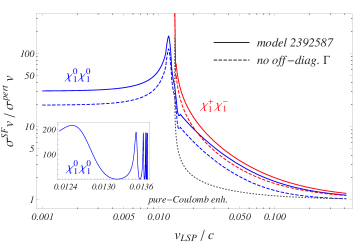
Figure 17: The enhancement of the $\chi^{0}_{1}\chi^{0}_{1}$ and $\chi^{+}_{1}\chi^{-}_{1}$ annihilation cross sections for Snowmass model $2392587$ relative to the perturbative tree-level rate, $(\sigma^{\rm SF}v)/(\sigma^{\rm pert}v)$. The solid lines refer to the calculation of the Sommerfeld-enhanced rates with off-diagonal entries in the annihilation matrices included. The dashed curves show the enhancement with respect to the perturbative cross sections when off-diagonal annihilation rates are not considered. The dotted curve labelled “pure–Coulomb enh.” shows the enhancement from photon exchange only in the $\chi^{+}_{1}\chi^{-}_{1}$ channel. Figure from [168].

In Figure 17 we plot the ratio $(\sigma^{\rm SF}v)/(\sigma^{\rm pert}v)$ of annihilation rates including long-range interactions, $\sigma^{\rm SF}v$, over the perturbative tree-level result, $\sigma^{\rm pert}v$, for the two-particle states $\chi^{0}_{1}\chi^{0}_{1}$ and $\chi^{+}_{1}\chi^{-}_{1}$ in the neutral sector of the model as a function of the velocity $v_{\rm LSP}$ of the incoming $\chi^{0}_{1}$’s in their centre-of-mass frame. The enhancement peaks in the vicinity of the threshold of the heavier neutral state $\chi^{+}_{1}\chi^{-}_{1}$ at $v_{\rm LSP}\simeq 0.014$. Well below this threshold, the enhancement for the $\chi^{0}_{1}\chi^{0}_{1}$ system is velocity-independent and of $\mathcal{O}(10)$.

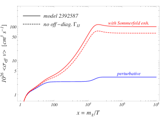
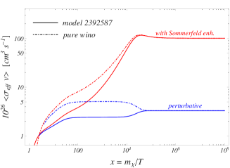
Figure 18: Upper panel: The thermally averaged effective annihilation rate $\langle\sigma_{\rm eff}v\rangle$ as a function of the scaled inverse temperature $x=m_{\chi}/T$ for Snowmass model $2392587$. The two upper (red) curves correspond to the Sommerfeld-enhanced annihilation cross sections including (solid line) or neglecting (dashed line) the off-diagonals in the annihilation matrices. The lower (blue) curve represents $\langle\sigma_{\rm eff}v\rangle$ obtained from perturbative (tree-level) cross sections. Lower panel: Comparison of $\langle\sigma_{\rm eff}v\rangle$ for model $2392587$ (solid) with the corresponding pure-wino scenario (dot-dashed). Figures from [168].

The quantity that enters the Boltzmann equation for the neutralino number density is the thermally averaged effective annihilation rate summed over all co-annihilation channels, $\langle\sigma_{\rm eff}v\rangle$. The upper panel of Figure 18 shows $\langle\sigma_{\rm eff}v\rangle$ as a function of the inverse scaled temperature $x=m_{\chi^{0}_{1}}/T$. As the temperature decreases, the Sommerfeld enhancement increases and reaches two orders of magnitude. Around $x\gtrsim 10^{4}$ the number densities of the $\chi^{\pm}_{1}$ are so strongly Boltzmann-suppressed with respect to the $\chi^{0}_{1}$ number density despite the small mass splitting that the rates of the charginos basically play no role in the effective rate $\langle\sigma_{\rm eff}v\rangle$, which is then essentially given by $\chi^{0}_{1}\chi^{0}_{1}$ annihilations. After $\chi^{\pm}_{1}$ decoupling, $\langle\sigma_{\rm eff}v\rangle$ including the Sommerfeld enhancements becomes constant, which we can infer from the constant enhancement factor for the $\chi^{0}_{1}\chi^{0}_{1}$ system for very low velocities shown in Figure 17. The difference between the dashed and solid lines in Figure 17 and the upper part of Figure 18 demonstrates that it is important to include correctly the off-diagonal annihilation reactions.

Since the lightest neutralino is almost a pure wino, the qualitative features of model $2392587$ are similar to the pure-wino studied already in [153]. There are, however, quantitative differences. A pure-wino model contains only an SU$(2)_{L}$ triplet of $\chi$ states in addition to the SM particles, while the MSSM model $2392587$ features non-decoupled sfermion states at the $2-3\,$TeV scale with non-vanishing couplings of the $\chi^{0}_{1}$ and $\chi^{\pm}_{1}$ to sfermions and to the (heavier) Higgs states, which reduce some of the annihilation rates relative to the pure-wino dark matter case. The difference of the thermally averaged effective annihilation rate for the two models, chosen to have the same $\chi_{1}^{0}$ mass, is shown in the lower panel of Figure 18.

The $\mathcal{O}(10^{2})$ effect seen in Figure 18 at large $x$ is not relevant to the dark-matter relic density computation, since freeze-out occurs already at $x\sim 20$. Nevertheless, the abundance is significantly modified. It is customary to solve the Boltzmann equation that determines the relic density for the yield $Y=n/s$, defined as the ratio of the number density $n$ of all co-annihilating particle species divided by the entropy density $s$ in the cosmic co-moving frame. Figure 19 shows the ratio of the yield $Y$ calculated from Sommerfeld-enhanced cross sections in both the pMSSM and the pure-wino model to the corresponding results using perturbative cross sections, $Y_{\rm pert}$, as a function of $x$. Around $x\sim 20$ the yields including Sommerfeld enhancements start to depart from the corresponding perturbative results. The enhanced annihilation rates delay the freeze-out of interactions, which leads to a reduction of the yield $Y$ compared to the perturbative result $Y_{\rm pert}$. The most drastic reduction in $Y/Y_{\rm pert}$ occurs between $x\sim 20$ and $x\sim 10^{3}$. In this region the enhancement factors on the cross sections are of $\mathcal{O}(10)$ (and not yet $\mathcal{O}(10^{2})$ as for very large $x$). Eventually, for $x\gtrsim 10^{5}$ the particle abundances in both the perturbative and Sommerfeld-enhanced calculation are frozen in, and the fraction $Y/Y_{\rm pert}$ remains constant. In case of the wino-like model we find that the relic densities calculated from the yield today read $\Omega^{\rm pert}h^{2}=0.112$ and $\Omega^{\rm SF}h^{2}=0.066$. Hence, the Sommerfeld effect leads to a reduction of the calculated relic abundance of around $40\%$ in this model. Neglecting the off-diagonal annihilations in the calculation would underestimate the effect considerably (dashed curve in Figure 19).

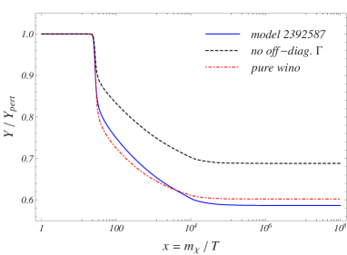
Figure 19: The ratios of the yield $Y/Y_{\rm pert}$ as a function of $x=m_{\chi^{0}_{1}}/T$, where $Y$ is calculated including the Sommerfeld enhancement on the $\chi\chi$ annihilation rates while $Y_{\rm pert}$ just uses the perturbative ones. The solid (blue) and dashed (black) curves give the results for the Snowmass model $2392587$ including and neglecting off-diagonal annihilation rates, respectively. The dot-dashed (red) curve corresponds to $Y/Y_{\rm pert}(x)$ in the pure-wino model. Figure from [168].

5.3.2 Higgsino-to-wino trajectory

The formalism described above allows us to consider lightest neutralino states, which are arbitrary admixtures of the electroweak gauginos and Higgsinos. Ref. [168] defines a “trajectory” in the $\mu$ and $M_{2}$ MSSM parameter space, which interpolates between an almost pure-Higgsino ($M_{2}\gg\mu$) and almost pure wino ($\mu\gg M_{2}$). A large bino fraction is excluded by choosing $M_{1}=10M_{2}$. The trajectory is then chosen such that the perturbative relic density computed with the program DarkSUSY [174] agrees with the most accurate determination obtained from the combination of PLANCK, WMAP, BAO and high resolution CMB data, $\Omega_{\rm cdm}h^{2}=0.1187\pm 0.0017$. The position of 13 models on this trajectory in the $\mu-M_{2}$ plane is shown in Figure 20. For details on the other MSSM parameters and the one-loop mass renormalization scheme, see [168]. The models can be categorized as higgsino-like with a wino fraction of $\chi^{0}_{1}$ below $10\%$ but a higgsino fraction $|Z_{N\,31}|^{2}+|Z_{N\,41}|^{2}$ above $0.9$ (models $1-6$), mixed wino-higgsino $\chi^{0}_{1}$ where both the wino and the higgsino fraction lie within $0.1-0.9$ (models $7-9$), or predominantly wino-like $\chi^{0}_{1}$ with wino fraction above $0.9$ (models $10-13$).

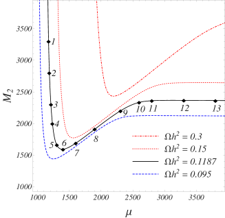
Figure 20: The $\mu-M_{2}$ plane with the $13$ models defining the higgsino-to-wino trajectory, indicated with diamonds. All trajectory models lie on the iso-contour for constant relic density $\Omega^{\rm DS}h^{2}=0.1187$ calculated with DarkSUSY. As reference we also show the iso-contours of constant relic densities $\Omega^{\rm DS}h^{2}=0.095$ (lowermost contour-line) $0.15$ and $0.3$ (uppermost iso-contour). Figure from [168].

For each of these models the relic density is computed perturbatively as well as with the Sommerfeld enhancement included in the non-relativistic effective theory approach discussed above. The result of this study is shown in Figure 21. For the higgsino-like and mixed models, the perturbative relic densities $\Omega^{\rm pert}h^{2}$ agree very well with the ones calculated with DarkSUSY for the same set of input parameters. For the wino-like models a difference of up to $8\%$ is observed. The Sommerfeld effect is measured by the height of the solid-hatched (red) bars, which give $\Omega^{\rm SF}h^{2}$, relative to the full height, which represents $\Omega^{\rm pert}h^{2}$. The difference between the two is generally below 10% for the most Higgsino-like model $1-5$, in agreement with the findings for pure-Higgsino models discussed in the context of Minimal Dark Matter [162]. The effect becomes more and more significant as the wino fraction increases, reaches a maximum for model 10, and then decreases again. For model 10, $\Omega^{\rm SF}h^{2}/\Omega^{\rm pert}h^{2}=0.394$, which implies that the relic density is overestimated by a factor 2.5, when the Sommerfeld effect is neglected. The occurrence of the maximal effect at parameter point 10, which features a lightest neutralino mass $m_{\rm LSP}=2320.986\,$GeV, can be attributed to the above-mentioned zero-energy resonance [152] in the Yukawa potential of the $\chi^{0}_{1}\chi^{0}_{1}$ annihilation channel.

These results demonstrate that it will be necessary to systematically include the Sommerfeld effect when MSSM parameter space constraints on heavy-neutralino dark matter from direct and indirect searches as well as from collider physics are combined with the requirement to reproduce, or at least not exceed, the observed abundance of dark matter. The formalism and tools developed in [165, 166, 167, 168] make it possible to investigate the parameter space of the general MSSM, and to identify regions where the Sommerfeld effect is not necessarily as pronounced as in the previously studied wino limit but still constitutes the dominant radiative correction.

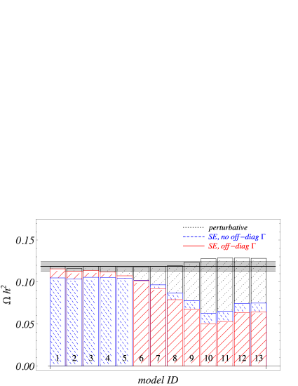
Figure 21: Relic densities $\Omega h^{2}$ for models $1-13$ on the higgsino-to-wino trajectory. The charts with dotted (black) hatching are the perturbative results $\Omega^{\rm pert}h^{2}$. Bars with dashed (blue) and solid-line (red) hatching refer to a calculation with Sommerfeld-enhanced cross sections neglecting and properly including off-diagonal rates, respectively. The grey shaded band comprises $\Omega h^{2}$ values within $5\%$ around the mean experimental value $\Omega_{\rm cdm}h^{2}=0.1187$. The latter value is indicated by the black horizontal line and agrees with the DarkSUSY result for all $13$ MSSM models on the trajectory. Figure from [168].

6 Summary

Non-relativistic physics and its effective description play an important role in many different areas of modern particle physics both in the electroweak and in the strong sector. The field of application reaches from precision determination of SM parameters, to the calculation of cross sections near thresholds for lepton or hadron collider reactions to high order in perturbation theory, and to the description of DM annihilation processes in the early Universe.

In this article we reviewed the production of heavy particles close to threshold within the framework of perturbative QCD. Special emphasis was put on top-quark pair production both at a future electron-positron collider but also at hadron colliders like the Tevatron and the LHC. We explained in detail the required methods and described the construction of the effective Lagrangians for the effective theories NRQCD and PNRQCD.

The envisaged experimental accuracy for the measurement of the total cross section $\sigma(e^{+}e^{-}\to t\bar{t})$ requires perturbative calculations up to the third order. We discussed several ingredients in detail and described the construction of the cross section. Due to the broad spectrum of required techniques, which range from three-loop vertex corrections in full QCD to the application of non-relativistic perturbation theory to third order including the corresponding ultrasoft effects, this project, now completed, can be considered as a benchmark calculation in the area of perturbative quantum field theory.

The hadroproduction of top quarks discussed in this review relies to a large extent on a factorization formula which separates hard and soft scales and the contributions from the potential region. It is utilized to perform a simultaneous resummation of Coulomb effects and soft-gluon radiation, which, in combination with the fixed-order NNLO result, leads to precise predictions for the total cross section. The same formalism is also applied to the pair production of supersymmetric particles.

Pair annihilation of heavy, weakly interacting dark matter particles opens a new and fascinating area of non-relativistic physics. Non-relativistic enhancements of the annihilation rate can be very large despite the fact that the force is generated by the exchange of electroweak gauge bosons. With TeV scale dark matter particles, degeneracies within the electroweak multiplet of DM are generic, leading to a complicated multi-channel Schrödinger problem. In this article we described the formulation and solution of this problem in the non-relativistic effective field theory framework with applications to neutralino dark matter of the minimal supersymmetric standard model.

References

References

- [1] M. Beneke, V. A. Smirnov, Asymptotic expansion of Feynman integrals near threshold, Nucl. Phys. B522 (1998) 321–344. arXiv:hep-ph/9711391.
- [2] B. Jantzen, Foundation and generalization of the expansion by regions, JHEP 1112 (2011) 076. arXiv:1111.2589.
- [3] B. A. Thacker, G. P. Lepage, Heavy quark bound states in lattice QCD, Phys. Rev. D43 (1991) 196–208.
- [4] G. P. Lepage, L. Magnea, C. Nakhleh, U. Magnea, K. Hornbostel, Improved nonrelativistic QCD for heavy quark physics, Phys. Rev. D46 (1992) 4052–4067. arXiv:hep-lat/9205007.
- [5] G. T. Bodwin, E. Braaten, G. P. Lepage, Rigorous QCD analysis of inclusive annihilation and production of heavy quarkonium, Phys.Rev. D51 (1995) 1125–1171. arXiv:hep-ph/9407339.
- [6] M. Beneke, Y. Kiyo, K. Schuller, Third-order correction to top-quark pair production near threshold I. Effective theory set-up and matching coefficients, arXiv:1312.4791.
- [7] A. Pineda, J. Soto, Effective field theory for ultrasoft momenta in NRQCD and NRQED, Nucl. Phys. Proc. Suppl. 64 (1998) 428–432. arXiv:hep-ph/9707481.
- [8] A. Pineda, J. Soto, The Lamb Shift in Dimensional Regularization, Phys. Lett. B420 (1998) 391–396. arXiv:hep-ph/9711292.
- [9] M. Beneke, New results on heavy quarks near threshold, arXiv:hep-ph/9806429.
- [10] N. Brambilla, A. Pineda, J. Soto, A. Vairo, Potential NRQCD: An effective theory for heavy quarkonium, Nucl. Phys. B566 (2000) 275. arXiv:hep-ph/9907240.
- [11] M. Beneke, A. Signer, V. A. Smirnov, Top quark production near threshold and the top quark mass, Phys.Lett. B454 (1999) 137–146. arXiv:hep-ph/9903260.
- [12] P. Marquard, J. Piclum, D. Seidel, M. Steinhauser, Completely automated computation of the heavy-fermion corrections to the three-loop matching coefficient of the vector current, Phys.Lett. B678 (2009) 269–275. arXiv:0904.0920.
- [13] P. Nogueira, Automatic Feynman graph generation, J.Comput.Phys. 105 (1993) 279–289.
- [14] R. Harlander, T. Seidensticker, M. Steinhauser, Complete corrections of Order alpha alpha-s to the decay of the Z boson into bottom quarks, Phys.Lett. B426 (1998) 125–132. arXiv:hep-ph/9712228.
- [15] T. Seidensticker, Automatic application of successive asymptotic expansions of Feynman diagramsarXiv:hep-ph/9905298.
- [16] J. Vermaseren, New features of FORM, arXiv:math-ph/0010025.
- [17] J. Kuipers, T. Ueda, J. Vermaseren, J. Vollinga, FORM version 4.0, Comput.Phys.Commun. 184 (2013) 1453–1467. arXiv:1203.6543.
- [18] S. Laporta, High precision calculation of multiloop Feynman integrals by difference equations, Int.J.Mod.Phys. A15 (2000) 5087–5159. arXiv:hep-ph/0102033.
- [19] A. Smirnov, M. Tentyukov, Feynman Integral Evaluation by a Sector decomposiTion Approach (FIESTA), Comput.Phys.Commun. 180 (2009) 735–746. arXiv:0807.4129.
- [20] A. Smirnov, V. Smirnov, M. Tentyukov, FIESTA 2: Parallelizeable multiloop numerical calculations, Comput.Phys.Commun. 182 (2011) 790–803. arXiv:0912.0158.
- [21] A. V. Smirnov, FIESTA 3: cluster-parallelizable multiloop numerical calculations in physical regions, Comput.Phys.Commun. 185 (2014) 2090–2100. arXiv:1312.3186.
- [22] V. S. Fadin, V. A. Khoze, Threshold Behavior of Heavy Top Production in e+ e- Collisions, JETP Lett. 46 (1987) 525–529.
- [23] O. I. Yakovlev, Top quark production near threshold: NNLO QCD correction, Phys.Lett. B457 (1999) 170–176. arXiv:hep-ph/9808463.
- [24] K. Melnikov, A. Yelkhovsky, Top quark production at threshold with accuracy, Nucl.Phys. B528 (1998) 59–72. arXiv:hep-ph/9802379.
- [25] A. Hoang, T. Teubner, Top quark pair production at threshold: Complete next-to-next-to-leading order relativistic corrections, Phys.Rev. D58 (1998) 114023. arXiv:hep-ph/9801397.
- [26] A. Hoang, T. Teubner, Top quark pair production close to threshold: Top mass, width and momentum distribution, Phys.Rev. D60 (1999) 114027. arXiv:hep-ph/9904468.
- [27] T. Nagano, A. Ota, Y. Sumino, corrections to total and differential cross-sections near threshold, Phys.Rev. D60 (1999) 114014. arXiv:hep-ph/9903498.
- [28] A. Penin, A. Pivovarov, Top quark threshold production in gamma gamma collision in the next-to-leading order, Nucl.Phys. B550 (1999) 375–396. arXiv:hep-ph/9810496.
- [29] A. H. Hoang, et al., Top-antitop pair production close to threshold: Synopsis of recent NNLO results, Eur. Phys. J. direct C2 (2000) 1. arXiv:hep-ph/0001286.
- [30] M. Beneke, A. Signer, V. A. Smirnov, Two-loop correction to the leptonic decay of quarkonium, Phys. Rev. lett. 80 (1998) 2535–2538. arXiv:hep-ph/9712302.
- [31] A. G. Kallen, A. Sabry, Fourth order vacuum polarization, Kong.Dan.Vid.Sel.Mat.Fys.Med. 29 (17) (1955) 1–20.
- [32] A. Czarnecki, K. Melnikov, Two-loop QCD corrections to the heavy quark pair production cross section in annihilation near the threshold, Phys. Rev. lett. 80 (1998) 2531–2534. arXiv:hep-ph/9712222.
- [33] B. Kniehl, A. Onishchenko, J. Piclum, M. Steinhauser, Two-loop matching coefficients for heavy quark currents, Phys.Lett. B638 (2006) 209–213. arXiv:hep-ph/0604072.
- [34] E. Braaten, Y.-Q. Chen, Renormalons in electromagnetic annihilation decays of quarkonium, Phys.Rev. D57 (1998) 4236–4253. arXiv:hep-ph/9710357.
- [35] P. Marquard, J. H. Piclum, D. Seidel, M. Steinhauser, Fermionic corrections to the three-loop matching coefficient of the vector current, Nucl. Phys. B758 (2006) 144–160. arXiv:hep-ph/0607168.
- [36] P. Marquard, J. H. Piclum, D. Seidel, M. Steinhauser, Three-loop matching of the vector current, Phys.Rev. D89 (2014) 034027. arXiv:1401.3004.
- [37] R. J. Guth, J. H. Kuhn, Top quark threshold and radiative corrections, Nucl. Phys. B368 (1992) 38–56.
- [38] D. Eiras, M. Steinhauser, Complete Higgs mass dependence of top quark pair threshold production to order alpha alpha(s), Nucl. Phys. B757 (2006) 197–210. arXiv:hep-ph/0605227.
- [39] Y. Kiyo, D. Seidel, M. Steinhauser, O(alpha alpha(s)) corrections to the gamma t anti-t vertex at the top quark threshold, JHEP 0901 (2009) 038. arXiv:0810.1597, doi:10.1088/1126-6708/2009/01/038.
- [40] Y. Kiyo, M. Steinhauser, N. Zerf, Supersymmetric Corrections to the Threshold Production of Top Quark Pairs, Phys.Rev. D80 (2009) 075005. arXiv:0907.1146.
- [41] P. Marquard, D. Seidel, unpublished.
- [42] J. Piclum, Heavy quark threshold dynamics in higher order, Ph.D. thesis, University of Hamburg (2007).
- [43] B. A. Kniehl, A. A. Penin, M. Steinhauser, V. A. Smirnov, Nonabelian heavy-quark-antiquark potential, Phys. Rev. D65 (2002) 091503. arXiv:hep-ph/0106135.
- [44] M. Beneke, Y. Kiyo, P. Marquard, A. Penin, J. Piclum, D. Seidel, M. Steinhauser, Leptonic decay of the Upsilon(1S) meson at third order in QCD, Phys.Rev.Lett. 112 (2014) 151801. arXiv:1401.3005.
- [45] A. V. Smirnov, V. A. Smirnov, M. Steinhauser, Fermionic contributions to the three-loop static potential, Phys. Lett. B668 (2008) 293–298. arXiv:0809.1927.
- [46] A. V. Smirnov, V. A. Smirnov, M. Steinhauser, Three-loop static potential, Phys. Rev. Lett. 104 (2010) 112002. arXiv:0911.4742.
- [47] C. Anzai, Y. Kiyo, Y. Sumino, Static QCD potential at three-loop order, Phys. Rev. Lett. 104 (2010) 112003. arXiv:0911.4335.
- [48] S. Larin, F. Tkachov, J. Vermaseren, The FORM version of MINCER.
- [49] K. Chetyrkin, F. Tkachov, Integration by Parts: The Algorithm to Calculate beta Functions in 4 Loops, Nucl.Phys. B192 (1981) 159–204.
- [50] A. Smirnov, Algorithm FIRE – Feynman Integral REduction, JHEP 0810 (2008) 107. arXiv:0807.3243.
- [51] A. Smirnov, V. Smirnov, FIRE4, LiteRed and accompanying tools to solve integration by parts relations, Comput.Phys.Commun. 184 (2013) 2820–2827. arXiv:1302.5885.
- [52] A. V. Smirnov, FIRE5: a C++ implementation of Feynman Integral REductionarXiv:1408.2372.
- [53] K. Chetyrkin, A. Kataev, F. Tkachov, New Approach to Evaluation of Multiloop Feynman Integrals: The Gegenbauer Polynomial x Space Technique, Nucl.Phys. B174 (1980) 345–377.
- [54] D. Kazakov, Calculation of Feynman integrals by the method of uniqueness, Theor.Math.Phys. 58 (1984) 223–230.
- [55] S. Bekavac, Calculation of massless Feynman integrals using harmonic sums, Comput.Phys.Commun. 175 (2006) 180–195. arXiv:hep-ph/0505174.
- [56] A. V. Smirnov, V. A. Smirnov, M. Steinhauser, The Static quark potential to three loops in perturbation theory, Nucl.Phys.Proc.Suppl. 205-206 (2010) 320–325. arXiv:1006.5513.
- [57] A. V. Smirnov, V. A. Smirnov, M. Steinhauser, Full Result for the Three-Loop Static Quark Potential, PoS RADCOR2009 (2010) 075. arXiv:1001.2668.
- [58] C. Anzai, Y. Sumino, Algorithms to Evaluate Multiple Sums for Loop Computations, J.Math.Phys. 54 (2013) 033514. arXiv:1211.5204.
- [59] T. Appelquist, M. Dine, I. Muzinich, The Static Limit of Quantum Chromodynamics, Phys.Rev. D17 (1978) 2074.
- [60] W. Fischler, Quark - anti-Quark Potential in QCD, Nucl. Phys. B129 (1977) 157–174.
- [61] A. Billoire, How Heavy Must Be Quarks in Order to Build Coulombic q anti-q Bound States, Phys. Lett. B92 (1980) 343.
- [62] M. Peter, The static quark-antiquark potential in QCD to three loops, Phys. Rev. Lett. 78 (1997) 602–605. arXiv:hep-ph/9610209.
- [63] Y. Schroder, The static potential in QCD to two loops, Phys. Lett. B447 (1999) 321–326. arXiv:hep-ph/9812205.
- [64] N. Brambilla, X. Garcia i Tormo, J. Soto, A. Vairo, The logarithmic contribution to the QCD static energy at NNNNLO, Phys. Lett. B647 (2007) 185. arXiv:hep-ph/0610143.
- [65] B. Kniehl, A. Penin, Y. Schroder, V. A. Smirnov, M. Steinhauser, Two-loop static QCD potential for general colour state, Phys.Lett. B607 (2005) 96–100. arXiv:hep-ph/0412083.
- [66] C. Anzai, M. Prausa, A. V. Smirnov, V. A. Smirnov, M. Steinhauser, Color octet potential to three loops, Phys.Rev. D88 (5) (2013) 054030. arXiv:1308.1202.
- [67] M. B. Voloshin, Precoulombic asymptotics for energy levels of heavy quarkonium, Sov. J. Nucl. Phys. 36 (1982) 143.
- [68] M. B. Voloshin, Nonperturbative effects in hadronic annihilation of heavy quarkonium, Sov. J. Nucl. Phys. 40 (1984) 662–667.
- [69] M. Beneke, Y. Kiyo, K. Schuller, Third-order Coulomb corrections to the S-wave Green function, energy levels and wave functions at the origin, Nucl. Phys. B714 (2005) 67–90. arXiv:hep-ph/0501289.
- [70] M. Beneke, Y. Kiyo, K. Schuller, Third-order correction to top-quark pair production near threshold II. Potential contributions, to appear.
- [71] M. Beneke, Y. Kiyo, K. Schuller, Third-order non-Coulomb correction to the S-wave quarkonium wave functions at the origin, Phys. Lett. B658 (2008) 222–229. arXiv:0705.4518.
- [72] M. Beneke, Y. Kiyo, K. Schuller, NNNLO results on top-quark pair production near threshold, arXiv:0801.3464.
- [73] M. Beneke, Y. Kiyo, Ultrasoft contribution to heavy-quark pair production near threshold, Phys.Lett. B668 (2008) 143–147. arXiv:0804.4004.
- [74] M. Beneke, Y. Kiyo, A. A. Penin, Ultrasoft contribution to quarkonium production and annihilation, Phys. Lett. B653 (2007) 53–59. arXiv:0706.2733.
- [75] M. Beneke, Y. Kiyo, P. Marquard, A. Penin, J. Piclum, M. Steinhauser, Next-to-next-to-next-to-leading order QCD prediction for the top anti-top S-wave pair production cross section near threshold in annihilation. arXiv:1506.06864
- [76] M. Beneke, A quark mass definition adequate for threshold problems, Phys. Lett. B434 (1998) 115–125. arXiv:hep-ph/9804241.
- [77] M. Beneke, V. M. Braun, Heavy quark effective theory beyond perturbation theory: Renormalons, the pole mass and the residual mass term, Nucl. Phys. B426 (1994) 301–343. arXiv:hep-ph/9402364.
- [78] I. I. Y. Bigi, M. A. Shifman, N. G. Uraltsev, A. I. Vainshtein, The Pole mass of the heavy quark. Perturbation theory and beyond, Phys. Rev. D50 (1994) 2234–2246. arXiv:hep-ph/9402360.
- [79] A. Pineda, A. Signer, Heavy quark pair production near threshold with potential non-relativistic QCD, Nucl. Phys. B762 (2007) 67–94. arXiv:hep-ph/0607239.
- [80] A. H. Hoang, M. Stahlhofen, The Top-Antitop Threshold at the ILC: NNLL QCD Uncertainties, JHEP 1405 (2014) 121. arXiv:1309.6323.
- [81] M. Beneke, P. Falgari, C. Schwinn, A. Signer, G. Zanderighi, Four-fermion production near the W pair production threshold, Nucl. Phys. B792 (2008) 89–135. arXiv:0707.0773.
- [82] S. Actis, M. Beneke, P. Falgari, C. Schwinn, Dominant NNLO corrections to four-fermion production near the W-pair production threshold, Nucl. Phys. B807 (2009) 1–32. arXiv:0807.0102, doi:10.1016/j.nuclphysb.2008.08.006.
- [83] M. Beneke, J. Piclum, T. Rauh, P-wave contribution to third-order top-quark pair production near threshold, Nucl.Phys. B880 (2014) 414–434. arXiv:1312.4792.
- [84] I. I. Bigi, V. S. Fadin, V. A. Khoze, Stop near threshold, Nucl.Phys. B377 (1992) 461–479.
- [85] A. A. Penin, A. A. Pivovarov, Analytical results for and observables near the threshold up to the next- to-next-to-leading order of NRQCD, Phys. Atom. Nucl. 64 (2001) 275–293. arXiv:hep-ph/9904278.
- [86] J. H. Kuhn, T. Teubner, Axial contributions at the top threshold, Eur. Phys. J. C9 (1999) 221–228. arXiv:hep-ph/9903322.
- [87] M. Beneke, A. Maier, J. Piclum, T. Rauh, Higgs effects in top anti-top production near threshold in annihilation. arXiv:1506.06865.
- [88] M. Beneke, A. P. Chapovsky, A. Signer, G. Zanderighi, Effective theory approach to unstable particle production, Phys. Rev. Lett. 93 (2004) 011602. arXiv:hep-ph/0312331.
- [89] M. Beneke, A. P. Chapovsky, A. Signer, G. Zanderighi, Effective theory calculation of resonant high-energy scattering, Nucl. Phys. B686 (2004) 205–247. arXiv:hep-ph/0401002.
- [90] M. Beneke, B. Jantzen, P. Ruiz-Femenia, Electroweak non-resonant NLO corrections to in the resonance region, Nucl. Phys. B840 (2010) 186–213. arXiv:1004.2188.
- [91] A. A. Penin, J. H. Piclum, Threshold production of unstable top, JHEP 1201 (2012) 034. arXiv:1110.1970.
- [92] A. H. Hoang, C. J. Reisser, Electroweak absorptive parts in NRQCD matching conditions, Phys. Rev. D71 (2005) 074022. arXiv:hep-ph/0412258.
- [93] B. Jantzen, P. Ruiz-Femenia, NNLO non-resonant corrections to threshold top-pair production from e+ e- collisions: Endpoint-singular terms, Phys.Rev. D88 (2013) 054011. arXiv:1307.4337.
- [94] P. Ruiz-Femenia, First estimate of the NNLO nonresonant corrections to top-antitop threshold production at lepton colliders, Phys.Rev. D89 (9) (2014) 097501. arXiv:1402.1123.
- [95] M. Beneke, Unstable-particle effective field theory, to appear in: Advances in computational particle physics, Nucl.Phys. B (Proc. Suppl.) (2015).
- [96] G. Sterman, Summation of Large Corrections to Short Distance Hadronic Cross-Sections, Nucl. Phys. B281 (1987) 310.
- [97] S. Catani, L. Trentadue, Resummation of the QCD Perturbative Series for Hard Processes, Nucl. Phys. B327 (1989) 323.
- [98] N. Kidonakis, G. Oderda, G. Sterman, Evolution of color exchange in QCD hard scattering, Nucl. Phys. B531 (1998) 365–402. arXiv:hep-ph/9803241.
- [99] E. Laenen, J. Smith, W. L. van Neerven, All order resummation of soft gluon contributions to heavy quark production in hadron hadron collisions, Nucl. Phys. B369 (1992) 543–599.
- [100] E. L. Berger, H. Contopanagos, The Perturbative Resummed Series for Top Quark Production in Hadron Reactions, Phys. Rev. D54 (1996) 3085–3113. arXiv:hep-ph/9603326.
- [101] S. Catani, M. L. Mangano, P. Nason, L. Trentadue, The Resummation of Soft Gluon in Hadronic Collisions, Nucl. Phys. B478 (1996) 273–310. arXiv:hep-ph/9604351.
- [102] N. Kidonakis, G. Sterman, Subleading logarithms in QCD hard scattering, Phys. Lett. B387 (1996) 867–874.
- [103] N. Kidonakis, G. Sterman, Resummation for QCD hard scattering, Nucl. Phys. B505 (1997) 321–348. arXiv:hep-ph/9705234.
- [104] R. Bonciani, S. Catani, M. L. Mangano, P. Nason, NLL resummation of the heavy-quark hadroproduction cross- section, Nucl. Phys. B529 (1998) 424–450. arXiv:hep-ph/9801375.
- [105] M. Beneke, P. Falgari, C. Schwinn, Soft radiation in heavy-particle pair production: All-order colour structure and two-loop anomalous dimension, Nucl.Phys. B828 (2010) 69–101. arXiv:0907.1443.
- [106] M. Beneke, P. Falgari, C. Schwinn, Threshold resummation for pair production of coloured heavy (s)particles at hadron colliders, Nucl.Phys. B842 (2011) 414–474. arXiv:1007.5414.
- [107] M. Beneke, A. P. Chapovsky, M. Diehl, T. Feldmann, Soft-collinear effective theory and heavy-to-light currents beyond leading power, Nucl. Phys. B643 (2002) 431–476. arXiv:hep-ph/0206152.
- [108] M. Beneke, T. Feldmann, Multipole-expanded soft-collinear effective theory with non-abelian gauge symmetry, Phys. Lett. B553 (2003) 267–276. arXiv:hep-ph/0211358.
- [109] C. W. Bauer, D. Pirjol, I. W. Stewart, Soft-collinear factorization in effective field theory, Phys. Rev. D65 (2002) 054022. arXiv:hep-ph/0109045.
- [110] M. Beneke, P. Falgari, C. Schwinn, All-Order Colour Structure and Two-Loop Anomalous Dimension of soft Radiation in Heavy-Particle Pair Production at the LHC, PoS RADCOR2009 (2010) 011. arXiv:1001.4621.
- [111] Y. Kiyo, J. H. Kuhn, S. Moch, M. Steinhauser, P. Uwer, Top-quark pair production near threshold at LHC, Eur.Phys.J. C60 (2009) 375–386. arXiv:0812.0919.
- [112] K. Hagiwara, Y. Sumino, H. Yokoya, Bound-state Effects on Top Quark Production at Hadron Colliders, Phys. Lett. B666 (2008) 71–76. arXiv:0804.1014.
- [113] A. Kulesza, L. Motyka, Soft gluon resummation for the production of gluino-gluino and squark-antisquark pairs at the LHC, Phys. Rev. D80 (2009) 095004. arXiv:0905.4749.
- [114] T. Becher, M. Neubert, Threshold resummation in momentum space from effective field theory, Phys. Rev. Lett. 97 (2006) 082001. arXiv:hep-ph/0605050.
- [115] T. Becher, M. Neubert, B. D. Pecjak, Factorization and momentum-space resummation in deep- inelastic scattering, JHEP 01 (2007) 076. arXiv:hep-ph/0607228.
- [116] T. Becher, M. Neubert, G. Xu, Dynamical Threshold Enhancement and Resummation in Drell- Yan Production, JHEP 07 (2008) 030. arXiv:0710.0680.
- [117] M. Beneke, P. Falgari, S. Klein, C. Schwinn, Hadronic top-quark pair production with NNLL threshold resummation, Nucl.Phys. B855 (2012) 695–741. arXiv:1109.1536.
- [118] G. P. Korchemsky, A. V. Radyushkin, Infrared factorization, Wilson lines and the heavy quark limit, Phys. Lett. B279 (1992) 359–366. arXiv:hep-ph/9203222.
- [119] N. Kidonakis, Two-loop soft anomalous dimensions and NNLL resummation for heavy quark production, Phys. Rev. Lett. 102 (2009) 232003. arXiv:0903.2561.
- [120] M. Czakon, A. Mitov, G. Sterman, Threshold Resummation for Top-Pair Hadroproduction to Next-to-Next-to-Leading Log, Phys. Rev. D80 (2009) 074017. arXiv:0907.1790.
- [121] J. H. Kuhn, E. Mirkes, QCD corrections to toponium production at hadron colliders, Phys.Rev. D48 (1993) 179–189. arXiv:hep-ph/9301204.
- [122] A. Petrelli, M. Cacciari, M. Greco, F. Maltoni, M. L. Mangano, NLO production and decay of quarkonium, Nucl. Phys. B514 (1998) 245–309. arXiv:hep-ph/9707223.
- [123] S. Moch, P. Uwer, Theoretical status and prospects for top-quark pair production at hadron colliders, Phys. Rev. D78 (2008) 034003. arXiv:0804.1476.
- [124] M. Beneke, M. Czakon, P. Falgari, A. Mitov, C. Schwinn, Threshold expansion of the cross section at , Phys. Lett. B690 (2010) 483–490. arXiv:0911.5166.
- [125] M. Aliev, et al., – HATHOR – HAdronic Top and Heavy quarks crOss section calculatoR, Comput. Phys. Commun. 182 (2011) 1034–1046. arXiv:1007.1327.
- [126] M. Beneke, P. Falgari, S. Klein, C. Schwinn, Threshold expansion of massive coloured particle cross sections, Nucl.Phys.Proc.Suppl. 205-206 (2010) 20–24. arXiv:1009.4011.
- [127] M. Cacciari, M. Czakon, M. Mangano, A. Mitov, P. Nason, Top-pair production at hadron colliders with next-to-next-to-leading logarithmic soft-gluon resummation, Phys.Lett. B710 (2012) 612–622. arXiv:1111.5869.
- [128] V. Ahrens, A. Ferroglia, M. Neubert, B. D. Pecjak, L. L. Yang, Renormalization-Group Improved Predictions for Top-Quark Pair Production at Hadron Colliders, JHEP 1009 (2010) 097. arXiv:1003.5827.
- [129] V. Ahrens, A. Ferroglia, M. Neubert, B. D. Pecjak, L.-L. Yang, RG-improved single-particle inclusive cross sections and forward-backward asymmetry in production at hadron colliders, JHEP 1109 (2011) 070. arXiv:1103.0550.
- [130] N. Kidonakis, Next-to-next-to-leading soft-gluon corrections for the top quark cross section and transverse momentum distribution, Phys. Rev. D82 (2010) 114030. arXiv:1009.4935.
- [131] P. Bärnreuther, M. Czakon, A. Mitov, Percent Level Precision Physics at the Tevatron: First Genuine NNLO QCD Corrections to , Phys.Rev.Lett. 109 (2012) 132001. arXiv:1204.5201.
- [132] M. Czakon, P. Fiedler, A. Mitov, Total Top-Quark Pair-Production Cross Section at Hadron Colliders Through , Phys.Rev.Lett. 110 (2013) 252004. arXiv:1303.6254.
- [133] M. Beneke, P. Falgari, S. Klein, J. Piclum, C. Schwinn, et al., Inclusive Top-Pair Production Phenomenology with TOPIXS, JHEP 1207 (2012) 194. arXiv:1206.2454.
- [134] M. Czakon, A. Mitov, Top++: A Program for the Calculation of the Top-Pair Cross-Section at Hadron Colliders, Comput.Phys.Commun. 185 (2014) 2930. arXiv:1112.5675.
- [135] A. D. Martin, W. J. Stirling, R. S. Thorne, G. Watt, Parton distributions for the LHC, Eur. Phys. J. C63 (2009) 189–285. arXiv:0901.0002.
- [136] U. Langenfeld, S. Moch, P. Uwer, Measuring the running top-quark mass, Phys.Rev. D80 (2009) 054009. arXiv:0906.5273.
- [137] V. M. Abazov, et al., Determination of the pole and MSbar masses of the top quark from the cross section, Phys.Lett. B703 (2011) 422–427. arXiv:1104.2887.
- [138] S. Chatrchyan, et al., Determination of the top-quark pole mass and strong coupling constant from the t t-bar production cross section in pp collisions at = 7 TeV, Phys.Lett. B728 (2014) 496–517. arXiv:1307.1907.
- [139] M. Czakon, M. L. Mangano, A. Mitov, J. Rojo, Constraints on the gluon PDF from top quark pair production at hadron colliders, JHEP 1307 (2013) 167. arXiv:1303.7215.
- [140] S. Alekhin, J. Bluemlein, S. Moch, The ABM parton distributions tuned to LHC data, Phys.Rev. D89 (2014) 054028. arXiv:1310.3059.
- [141] A. Kulesza, L. Motyka, Threshold resummation for squark-antisquark and gluino-pair production at the LHC, Phys. Rev. Lett. 102 (2009) 111802. arXiv:0807.2405.
- [142] W. Beenakker, S. Brensing, M. Kramer, A. Kulesza, E. Laenen, et al., Soft-gluon resummation for squark and gluino hadroproduction, JHEP 0912 (2009) 041. arXiv:0909.4418.
- [143] K. Hagiwara, H. Yokoya, Bound-state effects on gluino-pair production at hadron colliders, JHEP 10 (2009) 049. arXiv:0909.3204.
- [144] M. R. Kauth, J. H. Kühn, P. Marquard, M. Steinhauser, Gluinonia: Energy Levels, Production and Decay, arXiv:0910.2612.
- [145] M. R. Kauth, J. H. Kuhn, P. Marquard, M. Steinhauser, Gluino Pair Production at the LHC: The Threshold, Nucl.Phys. B857 (2012) 28–64. arXiv:1108.0361.
- [146] P. Falgari, C. Schwinn, C. Wever, NLL soft and Coulomb resummation for squark and gluino production at the LHC, JHEP 1206 (2012) 052. arXiv:1202.2260.
- [147] P. Falgari, C. Schwinn, C. Wever, Finite-width effects on threshold corrections to squark and gluino production, JHEP 1301 (2013) 085. arXiv:1211.3408.
- [148] W. Beenakker, S. Brensing, M. Kramer, A. Kulesza, E. Laenen, et al., NNLL resummation for squark-antisquark pair production at the LHC, JHEP 1201 (2012) 076. arXiv:1110.2446.
- [149] M. Beneke, P. Falgari, J. Piclum, C. Schwinn, C. Wever, Higher-order soft and Coulomb corrections to squark and gluino production at the LHC, PoS RADCOR2013 (2013) 051. arXiv:1312.0837.
- [150] W. Beenakker, C. Borschensky, M. Krämer, A. Kulesza, E. Laenen, et al., NNLL resummation for squark and gluino production at the LHC, JHEP 1412 (2014) 023. arXiv:1404.3134.
- [151] T. Pfoh, Phenomenology of QCD threshold resummation for gluino pair production at NNLL, JHEP 1305 (2013) 044. arXiv:1302.7202.
- [152] J. Hisano, S. Matsumoto, M. M. Nojiri, O. Saito, Non-perturbative effect on dark matter annihilation and gamma ray signature from galactic center, Phys.Rev. D71 (2005) 063528. arXiv:hep-ph/0412403.
- [153] J. Hisano, S. Matsumoto, M. Nagai, O. Saito, M. Senami, Non-perturbative effect on thermal relic abundance of dark matter, Phys.Lett. B646 (2007) 34–38. arXiv:hep-ph/0610249.
- [154] N. Arkani-Hamed, D. P. Finkbeiner, T. R. Slatyer, N. Weiner, A Theory of Dark Matter, Phys.Rev. D79 (2009) 015014. arXiv:0810.0713.
- [155] A. Hryczuk, R. Iengo, P. Ullio, Relic densities including Sommerfeld enhancements in the MSSM, JHEP 1103 (2011) 069. arXiv:1010.2172.
- [156] M. Drees, J. Kim, K. Nagao, Potentially Large One-loop Corrections to WIMP Annihilation, Phys.Rev. D81 (2010) 105004. arXiv:0911.3795.
- [157] A. Hryczuk, The Sommerfeld enhancement for scalar particles and application to sfermion co-annihilation regions, Phys.Lett. B699 (2011) 271–275. arXiv:1102.4295.
- [158] A. Hryczuk, R. Iengo, The one-loop and Sommerfeld electroweak corrections to the Wino dark matter annihilation, JHEP 1201 (2012) 163. arXiv:1111.2916.
- [159] J. Fan, M. Reece, In Wino Veritas? Indirect Searches Shed Light on Neutralino Dark Matter, JHEP 1310 (2013) 124. arXiv:1307.4400.
- [160] T. Cohen, M. Lisanti, A. Pierce, T. R. Slatyer, Wino Dark Matter Under Siege, JCAP 1310 (2013) 061. arXiv:1307.4082.
- [161] A. Hryczuk, I. Cholis, R. Iengo, M. Tavakoli, P. Ullio, Indirect Detection Analysis: Wino Dark Matter Case Study, JCAP 1407 (2014) 031. arXiv:1401.6212.
- [162] M. Cirelli, A. Strumia, M. Tamburini, Cosmology and Astrophysics of Minimal Dark Matter, Nucl.Phys. B787 (2007) 152–175. arXiv:0706.4071.
- [163] M. Cirelli, J. M. Cline, Can multistate dark matter annihilation explain the high-energy cosmic ray lepton anomalies?, Phys.Rev. D82 (2010) 023503. arXiv:1005.1779.
- [164] D. P. Finkbeiner, L. Goodenough, T. R. Slatyer, M. Vogelsberger, N. Weiner, Consistent Scenarios for Cosmic-Ray Excesses from Sommerfeld-Enhanced Dark Matter Annihilation, JCAP 1105 (2011) 002. arXiv:1011.3082.
- [165] M. Beneke, C. Hellmann, P. Ruiz-Femenia, Non-relativistic pair annihilation of nearly mass degenerate neutralinos and charginos I. General framework and S-wave annihilation, JHEP 1303 (2013) 148. arXiv:1210.7928.
- [166] C. Hellmann, P. Ruiz-Femenia, Non-relativistic pair annihilation of nearly mass degenerate neutralinos and charginos II. P-wave and next-to-next-to-leading order S-wave coefficients, JHEP 1308 (2013) 084. arXiv:1303.0200.
- [167] M. Beneke, C. Hellmann, P. Ruiz-Femenia, Non-relativistic pair annihilation of nearly mass degenerate neutralinos and charginos III. Computation of the Sommerfeld enhancements, arXiv:1411.6924.
- [168] M. Beneke, C. Hellmann, P. Ruiz-Femenia, Heavy neutralino relic abundance with Sommerfeld enhancements - a study of pMSSM scenarios, arXiv:1411.6930.
- [169] J. Alwall, M. Herquet, F. Maltoni, O. Mattelaer, T. Stelzer, MadGraph 5 : Going Beyond, JHEP 1106 (2011) 128. arXiv:1106.0522.
- [170] A. Djouadi, J.-L. Kneur, G. Moultaka, SuSpect: A Fortran code for the supersymmetric and Higgs particle spectrum in the MSSM, Comput.Phys.Commun. 176 (2007) 426–455. arXiv:hep-ph/0211331.
- [171] T. R. Slatyer, The Sommerfeld enhancement for dark matter with an excited state, JCAP 1002 (2010) 028. arXiv:0910.5713.
- [172] S. Ershov, J. Vaagen, M. Zhukov, Modified variable phase method for the solution of coupled radial Schrödinger equations, Phys.Rev. C84 (2011) 064308.
- [173] M. W. Cahill-Rowley, J. L. Hewett, A. Ismail, M. E. Peskin, T. G. Rizzo, pMSSM Benchmark Models for Snowmass 2013, in: “A Community Summer Study 2013 : Snowmass on the Mississippi”, 29 Jul - 6 Aug 2013, Minneapolis, USA. arXiv:1305.2419.
- [174] P. Gondolo, J. Edsjo, P. Ullio, L. Bergstrom, M. Schelke, et al., DarkSUSY: Computing supersymmetric dark matter properties numerically, JCAP 0407 (2004) 008. arXiv:astro-ph/0406204.