Factorized Asymptotic Bayesian Inference for Factorial Hidden Markov Models

Abstract

Factorial hidden Markov models (FHMMs) are powerful tools of modeling sequential data. Learning FHMMs yields a challenging simultaneous model selection issue, i.e., selecting the number of multiple Markov chains and the dimensionality of each chain. Our main contribution is to address this model selection issue by extending Factorized Asymptotic Bayesian (FAB) inference to FHMMs. First, we offer a better approximation of marginal log-likelihood than the previous FAB inference. Our key idea is to integrate out transition probabilities, yet still apply the Laplace approximation to emission probabilities. Second, we prove that if there are two very similar hidden states in an FHMM, i.e. one is redundant, then FAB will almost surely shrink and eliminate one of them, making the model parsimonious. Experimental results show that FAB for FHMMs significantly outperforms state-of-the-art nonparametric Bayesian iFHMM and Variational FHMM in model selection accuracy, with competitive held-out perplexity.

1 Introduction

The Factorial Hidden Markov Model (FHMM) [8] is an extension of the Hidden Markov Model (HMM), in which the hidden states are factorized into several independent Markov chains, and emissions (observations) are determined by their combination. FHMMs have found successful applications in speech recognition [16], source separation [18, 15, 11, 12], natural language processing [4] and bioinformatics [10]. A graphical model representation of the FHMM is shown in Fig.1.

Figure 1: Graphical Model Representation of FHMMs.

Learning FHMMs naturally yields a challenging simultaneous model selection issue, i.e., how many independent Markov chains we need (layer-level model selection), and what is the dimensionality (number of hidden states) of each Markov chain. As the model space increases exponentially with the number of the Markov chains, it is not feasible to employ a grid search based method like cross-validation [2]. More sophisticated methods, like variational Bayesian inference (VB-FHMMs) [1] and the nonparametric Bayesian Infinite FHMMs (iFHMMs) [19] have been proposed, but they cannot fully address the issue. For example, iFHMMs restrict the dimensionality of each Markov chain to be binary. Further, high computational costs of VB-FHMMs and iFHMMs restrict their applicability to large scale problems.

This paper addresses the above model selection issue of FHMMs by extending Factorized Asymptotic Bayesian (FAB) inference, which is a recent model selection framework and has shown superior performance than nonparametric Bayesian inference for Mixture Models [7], Hidden Markov Models [6], Latent Feature Models [9], and Hierarchical Mixture of Experts Models [5]. Our method, namely $\text{FAB}_{fhmm}$, not only fully addresses the simultaneous model selection issue, but also offers the following two contributions.

1) Better marginal log-likelihood approximation with partial marginalization technique: Previous FAB inference for HMMs [6] has applied the Laplace approximations both to emission probabilities and to transition probabilities. Our approach applies the Laplace approximations only to emission probabilities, and transition probabilities are integrated out. As we do not conduct asymptotic approximation but follow exact marginalization on transition probabilities, we can better approximate marginal log-likelihood.

2) A quantitative analysis of the shrinkage process: One of the strong features in FAB inference is a shrinkage effect, caused by FAB-unique asymptotic regularization, on hidden variables , i.e., redundant hidden states are automatically removed during the FAB EM-like iterative optimization. Although its strong model selection capability has been empirically confirmed [7, 6, 9], its mathematical behavior has not been well studied. This paper carefully investigates the shrinkage process, and proves that if there are two very similar hidden states in FHMMs, then one state would almost surely “die out”. We reveal the following chain reaction between E-steps and M-steps: if the variational probabilities of some states are shrunk in an E-step, then their corresponding model parameters will also be shrunk in the next M-step, causing these state to be shrunk further in future E-steps. Moreover, under certain condition, this shrinkage process is accelerating. This finding also partially answers the parameter identifiability problem of FHMMs.

2 Related Work

2.1 Factorial HMMs

The pioneering work of FHMMs was by Z. Ghahramani and M. Jordan [8]. The idea of FHMMs is to express emissions (observations) by combining $M$ independent Markov chains. If the individual Markov chain have binary states, the FHMM can express $2^{M}$ different emission distributions. Their inference, structured variational inference, uses Baum-Welch algorithm [17] to learn parameters. Generally speaking, variational Bayesian (VB) inference [14, 1] can prune redundant latent states, but previous studies have suggested the pruning effect is not strong enough to achieve good model selection performance.

Recently, infinite FHMMs (iFHMMs) have been proposed [19] to address the model selection issue of FHMMs. iFHMMs employ the Markov Indian Buffet Process (mIBP) as the prior of the transition matrix of the infinite hidden states. Although iFHMMs offer strong model selection ability in learning FHMMs, they have a few limitations. First, iFHMMs restrict latent variables to be binary while the original FHMMs [8] have no such limitation. This restriction makes iFHMMs generate more represented states than variational methods, tending to overfit the data. In contrast, excluding such a restriction and allowing different Markov chains to have different numbers of hidden states may give us better understanding of the data. Second, the slice sampling used to optimize the iFHMM is considerably slower than variational methods, and therefore iFHMMs do not scale well to large scale scenarios.

2.2 FAB Inference

Factorized asymptotic Bayesian (FAB) inference has been originally proposed to address model selection of mixture models [7]. FAB inference selects the model which maximizes an asymptotic approximation of the marginal log-likelihood of the observed data, referred to as Factorized Information Criterion (FIC), with an EM-like iterative optimization procedure. Previous studies have extended FAB inference to HMMs (sequential) [6] and Latent Feature Models (factorial) [9], and have shown superiority against variational inference and nonparametric Bayesian methods in terms of model selection accuracy and computational cost. It is an interesting open challenge to investigate FAB inference for their intermediate (both sequential and factorial) models, i.e., FHMMs.

3 Factorial Hidden Markov Models

Suppose we have observed $N$ independent sequences, denoted as $\boldsymbol{x^{N}}=\boldsymbol{x}^{1},\cdots,\boldsymbol{x}^{N}$. The n-th sequence is denoted as $\boldsymbol{x}^{n}=\boldsymbol{x}_{1}^{n},\cdots,\boldsymbol{x}_{T_{n}}^{n}$, where $T_{n}$ is the length of the $n$-th sequence. Respectively, we denote the corresponding sequences of hidden state variables as $\boldsymbol{z^{N}}=\boldsymbol{z}^{1},\cdots,\boldsymbol{z}^{N}$, and each sequence $\boldsymbol{z}^{n}=\boldsymbol{z}_{1}^{n},\boldsymbol{z}_{2}^{n},\cdots,\boldsymbol{z}_{T_{n}}^{n}$. $\boldsymbol{z}_{t}^{n}$ consists of hidden variables of $M$ independent HMMs: $\boldsymbol{z}_{t}^{n}=\boldsymbol{z}_{t}^{n,(1)},\boldsymbol{z}_{t}^{n,(2)},\cdots,\boldsymbol{z}_{t}^{n,(M)}$. The $m$-th HMM has $K_{m}$ hidden states, i.e., $\boldsymbol{z}_{t}^{n,(m)}\in\{0,1\}^{K_{m}}$. We represent $\boldsymbol{z}_{t}^{n,(m)}$ as a $K_{m}\cdot 1$ binary vector, where the $k$-th component, $z_{t,k}^{n,(m)}$, denotes whether state $z_{t}^{n,(m)}=k$.

An FHMM model is specified as the following probability density:

$$p(\boldsymbol{x}^{n},\boldsymbol{z}^{n}|\boldsymbol{\theta})\!=\! \prod_{m=1}^{M}\!\!\Big{\{}p(\boldsymbol{z}_{1}^{n,(m)}|\boldsymbol{\alpha}^{m})\!\prod_{t=2}^{T_{n}}p(\boldsymbol{z}_{t}^{n,(m)}|\boldsymbol{z}_{t-1}^{n,(m)},\boldsymbol{\beta}^{m})\Big{\}}$$

$$\prod_{t=1}^{T}p(\boldsymbol{x}_{t}^{n}|\boldsymbol{z}_{t}^{n},\boldsymbol{\phi}),$$ (1)

where $\boldsymbol{\theta}=(\boldsymbol{\alpha},\boldsymbol{\beta},\boldsymbol{\phi})$. The initial, transition and emission distributions are represented as $p(\boldsymbol{z}_{1}^{(m)}|\boldsymbol{\alpha}^{m})$, $p(\boldsymbol{z}_{t}^{n,(m)}|\boldsymbol{z}_{t-1}^{n,(m)},\boldsymbol{\beta}^{m})$, and $p(\boldsymbol{x}_{t}^{n}|\boldsymbol{z}_{t}^{n},\boldsymbol{\phi})$, respectively.

The $m$-th initial and transition distributions are defined as follows:

• $p(\boldsymbol{z}_{1}^{(m)}|\boldsymbol{\alpha}^{(m)})=\prod_{k=1}^{K_{m}}(\alpha_{k}^{(m)})^{z_{1,k}^{(m)}}$;

• $p(\boldsymbol{z}_{t}^{(m)}|\boldsymbol{z}_{t-1}^{(m)},\boldsymbol{\beta}^{(m)})=\prod_{j,k=1}^{K_{m}}(\beta_{j,k}^{(m)})^{z_{t-1,j}z_{t,k}}$.

Here $\boldsymbol{\alpha}^{(m)}=(\alpha_{1}^{(m)},\cdots,\alpha_{K_{m}}^{(m)})$, with $\sum_{k=1}^{K_{m}}\alpha_{k}^{(m)}=1$; $\boldsymbol{\beta}^{(m)}=\left(\beta_{i,j}^{(m)}\right)$, with each row $\boldsymbol{\beta}_{k}^{(m)}$ summing to 1.

By following the original FHMM work [8], this paper considers multidimensional Gaussian emission, while it is not difficult to extend our discussion to more general distributions like one in the exponential family. The emission distribution is jointly parameterized across the hidden states in the $M$ HMMs as follows:

$$p(\boldsymbol{x}_{t}^{n}|\boldsymbol{z}_{t}^{n},\phi)=\mathcal{N}(\boldsymbol{x}_{t}^{n},\boldsymbol{\mu}_{t}^{n},\boldsymbol{C}),$$ (2)

where $\boldsymbol{\mu}_{t}^{n}$ and $\boldsymbol{C}$ are the mean vector and covariance matrix. A key idea (and difference from HMMs) in FHMMs is the construction of the mean vector $\boldsymbol{\mu}_{t}^{n}$. More specifically, the mean vector $\boldsymbol{\mu}_{t}^{n}$ is represented by the following linear combination:

$$\boldsymbol{\mu}_{t}^{n}= \sum_{m=1}^{M}\boldsymbol{W}^{m}\boldsymbol{z}_{t}^{n,(m)},$$ (3)

where $\boldsymbol{W}^{m}$ is a $D\times K_{m}$ matrix. The $k$-th row of $\boldsymbol{W}^{m}$ is denoted as $\boldsymbol{W}_{k}^{m}$, specifying the contribution of the $k$-th state in the $m$-th HMM to the mean. Here, $\phi$ in (1) can be represented as $\phi=(\boldsymbol{W},\boldsymbol{C})$.

4 Refined Factorized Information Criterion for FHMMs

FIC derivation starts from the following equivalent form of marginal log-likelihood: -1em

$$\log p(\boldsymbol{x^{N}}|\mathcal{M})\equiv\max_{q}\sum_{\boldsymbol{z^{N}}}q(\boldsymbol{z^{N}})\log(\frac{p(\boldsymbol{x^{N}},\boldsymbol{z^{N}}|\mathcal{M})}{q(\boldsymbol{z^{N}})})$$ (4)

$\mathcal{M}$ represents a model and $\mathcal{M}=(M,K_{1},\cdots,K_{M})$ in FHMMs. $q(\boldsymbol{z})$ is a variational distribution over the hidden states. For a state vector $\boldsymbol{z}{}_{t}^{n,m}$, its expectation under $q$, $\mathbf{E}_{q}[\boldsymbol{z}_{t}^{n,m}]$, is denoted in shorthand as $q(\boldsymbol{z}_{t}^{n,m})$, and the expectation of two consecutive states $\mathbf{E}_{q}[z_{t-1,j}^{n,m}\cdot z_{t,k}^{n,m}]$ as $q(z_{t-1,j}^{n,m},z_{t,k}^{n,m})$.

A direct application of the technique proposed in [7, 6] leads to the following asymptotic approximation of the complete marginal log-likelihood:

$$p(\boldsymbol{x^{N}}, \boldsymbol{z^{N}}|\mathcal{M})=\prod_{m=1}^{M}\Bigl{\{}\underbrace{\int p(\boldsymbol{z}_{1}^{(m)}|\boldsymbol{\alpha}^{m})p(\boldsymbol{\alpha}^{m}|\mathcal{M})d\boldsymbol{\alpha}^{m}}_{\textnormal{Laplace\ Approx}.}$$

$$\underbrace{\int\prod_{t=2}^{T_{n}}p(\boldsymbol{z}_{t}^{n,(m)}|\boldsymbol{z}_{t-1}^{n,(m)},\boldsymbol{\beta}^{m})p(\boldsymbol{\beta}^{m}|\mathcal{M})d\boldsymbol{\beta}^{m}}_{\textnormal{Laplace\ Approx}.}\Bigr{\}}$$

$$\underbrace{\int\prod_{t=1}^{T}p(\boldsymbol{x}_{t}^{n}|\boldsymbol{z}_{t}^{n},\boldsymbol{\phi})p(\boldsymbol{\phi}|\mathcal{M})d\boldsymbol{\phi}}_{\textnormal{Laplace\ Approx}.}.$$ (5)

Instead, this paper proposes the FIC derivation with integrating out the initial and transition distributions.

$$p(\boldsymbol{x^{N}}, \boldsymbol{z^{N}}|\mathcal{M})=\prod_{m=1}^{M}\Bigl{\{}\underbrace{\int p(\boldsymbol{z}_{1}^{(m)}|\boldsymbol{\alpha}^{m})p(\boldsymbol{\alpha}^{m}|\mathcal{M})d\boldsymbol{\alpha}^{m}}_{\text{Integrated \ Out}}$$

$$\underbrace{\int\prod_{t=2}^{T_{n}}p(\boldsymbol{z}_{t}^{n,(m)}|\boldsymbol{z}_{t-1}^{n,(m)},\boldsymbol{\beta}^{m})p(\boldsymbol{\beta}^{m}|\mathcal{M})d\boldsymbol{\beta}^{m}}_{\text{Integrated \ Out}}\Bigr{\}}$$

$$\underbrace{\int\prod_{t=1}^{T}p(\boldsymbol{x}_{t}^{n}|\boldsymbol{z}_{t}^{n},\boldsymbol{\phi})p(\boldsymbol{\phi}|\mathcal{M})d\boldsymbol{\phi}}_{\text{Laplace \ Approx.}}.$$ (6)

The original motivation of FIC is to approximate “intractable” Bayesian marginal log-likelihood. The key idea in (6) is to refine approximation by analytically solving the tractable integrations (w.r.t. $\alpha^{m}$ and $\boldsymbol{\beta}^{m}$) and minimizing the asymptotic approximation error.

After integrating out all the parameters, and normalizing the Hessians w.r.t. $\boldsymbol{W}$ and $\boldsymbol{C}^{-1}$, we obtain:

With uninformative conjugate priors on $\boldsymbol{\alpha}^{m}$ and $\boldsymbol{\beta}^{m}$, we can calculate (6) as follows:

$$p(\boldsymbol{x^{N}},\boldsymbol{z^{N}}|\mathcal{M})$$

$$\approx \prod_{m}\Big{(}\frac{\prod_{k}\Gamma(c_{m,0,k}+1)}{\Gamma(\sum_{k}c_{m,0,k}+K_{m})}\prod_{j}\frac{\prod_{k}\Gamma(c_{m,j,k}+1)}{\Gamma(\sum_{k}c_{m,j,k}+K_{m})}\Big{)}$$

$$\cdot\prod_{d=1}^{D}(2\pi)^{\frac{K_{0}+1}{2}}(\prod_{n=1}^{N}\frac{T_{n}}{2})^{-\frac{1}{2}}c_{d}^{-\frac{K_{0}-2}{2}}|\hat{\mathcal{F}}_{\mkern 1.5mu\overline{\mkern-1.5mu\boldsymbol{W}\mkern-1.5mu}\mkern 1.5mu_{d},\bar{c}_{d}}|^{-\frac{1}{2}}$$

$$\cdot\prod_{m,k=1}^{M,K_{m}}(\sum_{n,t=1}^{N,T_{n}}z_{t,k}^{n,(m)})^{-\frac{1}{2}},$$ (7)

where $K_{0}=\sum_{m}K_{m}$, and $\hat{\mathcal{F}}_{\mkern 1.5mu\overline{\mkern-1.5mu\boldsymbol{W}\mkern-1.5mu}\mkern 1.5mu_{d},\bar{c}_{d}}$ is the normalized Hessian w.r.t. the $d$-th rows of $\boldsymbol{W}$ and $\boldsymbol{C}^{-1}$ at the maximum likelihood estimators $\mkern 1.5mu\overline{\mkern-1.5mu\boldsymbol{W}\mkern-1.5mu}\mkern 1.5mu,\mkern 1.5mu\overline{\mkern-1.5mu\boldsymbol{C}\mkern-1.5mu}\mkern 1.5mu$. The normalization makes $|\hat{\mathcal{F}}_{\mkern 1.5mu\overline{\mkern-1.5mu\boldsymbol{W}\mkern-1.5mu}\mkern 1.5mu_{d},\bar{c}_{d}}|=O(1)$, by extracting the terms involving $\boldsymbol{z}$.

(4) computes the expectation of $\log p(\boldsymbol{x^{N}},\boldsymbol{z^{N}}|\mathcal{M})$ w.r.t. the variational distribution $q$. Taking the logarithm of (7), many log-Gamma terms appear, whose exact expectations require to enumerate the exponentially many possible configurations of $\boldsymbol{z}$, which is infeasible. Thus we propose a first-order approximation to them, based on the following lemmas, where $\epsilon_{1},\epsilon_{2},\epsilon_{3}$ are small bounded errors.

Lemma 1.

Suppose $\{z_{1}^{n},\cdots,z_{T_{n}}^{n}\}_{n=1}^{N}$ are $N$ sequences of Bernoulli random variables. Within each sequence, $\{z_{t}^{n}\}_{t=1}^{T_{n}}$ are independent with each other. Let $y_{n}=\sum_{i}z_{i}^{n}$, $\bar{y}_{n}=E[y_{n}]$. Besides, there are $N$ numbers $\{\hat{y}_{n}\}$, $\forall k,\hat{y}_{n}\approx\bar{y}_{n}$. When all $T_{n}$ are large enough:

1) $\mathbf{E}[\log\Gamma(y_{n})]=y_{n}\log\bar{y}_{n}-(\bar{y}_{n}+\frac{1}{2}\log\bar{y}_{n})+\log 2\pi+\epsilon_{1}.$

2) $\mathbf{E}\left[\operatornamewithlimits{{\sum}}_{n}\!\log\!\Gamma(y_{n})\!-\!\log\!\Gamma(\operatornamewithlimits{{\sum}}_{n}y_{n})\right]\!=\!\operatornamewithlimits{{\sum}}_{n}y_{n}\!\log\!\big{(}\frac{\hat{y}_{n}}{\operatornamewithlimits{{\sum}}_{m=1}^{N}\hat{y}_{m}}\big{)}\allowbreak+\frac{1}{2}\log\big{(}\operatornamewithlimits{{\sum}}_{n}\hat{y}_{n}\big{)}-\frac{1}{2}\operatornamewithlimits{{\sum}}_{n}\log\hat{y}_{n}+(N-1)\log 2\pi+\epsilon_{2}.$

3) $\mathbf{E}[\log y_{n}]=\log\hat{y}_{n}+\frac{1}{\hat{y}}(\bar{y}_{n}-\hat{y}_{n})+\epsilon_{3}.$

Proof can be found in the Appendix.

As defined above, $c_{m,j,k}=\sum_{n,t=1}^{N,T_{n}-1}z_{t,j}^{n,m}z_{t+1,k}^{n,m}$. Since $\{z_{t}^{n,m}\}_{t=1}^{T_{n}}$ follows a Markov process, the dependency between $z_{t,j}^{n,m}$ and $z_{t+\Delta t,j}^{n,m}$ vanishes quickly when the time gap $\Delta t$ increases, leading to the uncoupling between $z_{t,j}^{n,m}z_{t+1,k}^{n,m}$ and $z_{t+\Delta t,j}^{n,m}z_{t+1+\Delta t,k}^{n,m}$. Thus we can approximately regard $c_{m,j,k}$ as the sum of independent Bernoulli random variables, and therefore Lemma 1 apply. The same argument applies to $c_{m,0,k}$.

In order to avoid recursion relations w.r.t. $q$ during the inference, we introduce an auxiliary distribution $\hat{q}$, which is always close to $q$, in that $\hat{q}(z_{t,k}^{n,m})\approx q(z_{t,k}^{n,m}),\hat{q}(z_{t,j}^{n,m},z_{t+1,k}^{n,m})\approx q(z_{t,j}^{n,m},z_{t+1,k}^{n,m})$. The Gamma terms in (7) will be expanded about the expectations of their parameters w.r.t. $\hat{q}$. We will discuss how to choose $\hat{q}$ in Section 5.2.

Taking the logarithm of (7), applying Lemma 1, and dropping asymptotically small terms (including the determinants of the normalized Hessian matrices), we derive the approximation of $p(\boldsymbol{x^{N}},\boldsymbol{z^{N}}|\mathcal{M})$. Plugging it into (4), we obtain an asymptotic approximation of the lower bound of $\log p(\boldsymbol{x^{N}}|M)$:

$$\log p(\boldsymbol{x^{N}}|\mathcal{M})\mathcal{\geq J}(q,\boldsymbol{x^{N}})$$

$$\approx \sum q(\boldsymbol{z^{N}})\bigg{[}\sum_{n,t}\Big{(}\log p(\boldsymbol{x}_{t}^{n}|\boldsymbol{z}_{t}^{n},\mkern 1.5mu\overline{\mkern-1.5mu\boldsymbol{W}\mkern-1.5mu}\mkern 1.5mu,\mkern 1.5mu\overline{\mkern-1.5mu\boldsymbol{C}\mkern-1.5mu}\mkern 1.5mu)+\sum_{m,k}z_{t,k}^{n,m}\log\delta_{k}^{m}\Big{)}$$

$$+\sum_{m,n=1}^{M,N}\Big{(}\sum_{k}z_{0,k}^{n,m}\log\hat{\alpha}_{k}^{m}+\sum_{t=1}^{T_{n}-1}\sum_{j,k}z_{t,j}^{n,m}z_{t+1,k}^{n,m}\log\hat{\beta}_{j,k}^{m}\Big{)}$$

$$-\log q(\boldsymbol{z^{N}})\bigg{]}\underline{+\sum_{m,n,t}\log\Delta^{m}-\frac{D}{2}\sum_{m,k=1}^{M,K_{m}}\log(\hat{c}_{m,\cdot,k})}$$

$$\underline{-\frac{1}{2}\sum_{m,k}\log(\hat{c}_{m,0,k}+1)-\frac{1}{2}\sum_{m,j,k}\log(\hat{c}_{m,j,k}+1)}$$

$$\underline{+\frac{1}{2}\sum_{m,j}\log(\sum_{k}\hat{c}_{m,j,k}+K_{m})+\frac{1}{2}\sum_{m}\log(N+K_{m})}$$

$$\underline{+\frac{D}{2}\sum_{m}K_{m}+\sum_{m}(K_{m}^{2}-1)\log 2\pi+\epsilon,}$$ (8)

with the definitions

$$\hat{q}(z_{t,i}^{n,m}) =E_{q}(z_{t,i}^{n,m}),\quad q(z_{t,j}^{n,m},z_{t+1,k}^{n,m})=E_{q}(z_{t,j}^{n,m},z_{t+1,k}^{n,m}),$$

$$\hat{c}_{m,0,k} =\sum_{n=1}^{N}\hat{q}(z_{1,k}^{n,m}),\quad\hat{c}_{m,\cdot,k}=\sum_{n,t=1}^{N,T_{n}}\hat{q}(z_{t,k}^{n,m}),$$

$$\hat{c}_{m,j,k} =\sum_{n,t=1}^{N,T_{n}-1}\hat{q}(z_{t,j}^{n,m},z_{t+1,k}^{n,m}),\allowdisplaybreaks$$

$$\delta_{k}^{m} =\frac{1}{\Delta^{m}}\exp\{-\frac{D}{2\sum_{n,t=1}^{N,T_{n}}\hat{q}(z_{t,k}^{n,m})}\},$$

$$\hat{\alpha}_{k}^{m} =\frac{1+\sum_{n=1}^{N}\hat{q}(z_{1,k}^{n,m})}{K_{m}+N},$$

$$\hat{\beta}_{j,k}^{m} =\frac{1+\sum_{n,t=1}^{N,T_{n}-1}\hat{q}(z_{t,j}^{n,m},z_{t+1,k}^{n,m})}{K_{m}+\sum_{n,t=1}^{N,T_{n}-1}q(z_{t,j}^{n,m})},$$ (9)

and $\Delta^{m}$ is a normalization constant that makes $\sum_{k=1}^{K_{m}}\delta_{k}^{m}=1$, $\varepsilon$ is a small constant error bound of the approximations. Note the ML estimators $\mkern 1.5mu\overline{\mkern-1.5mu\boldsymbol{W}\mkern-1.5mu}\mkern 1.5mu,\mkern 1.5mu\overline{\mkern-1.5mu\boldsymbol{C}\mkern-1.5mu}\mkern 1.5mu$ inside the summation are subject to the specific instantiation of $\boldsymbol{z^{N}}$.

In (9), $\hat{\alpha}$ and $\hat{\beta}$ can be viewed as the estimated initial transition probabilities of the FHMM w.r.t. $\hat{q}$.

The FIC of the FHMM, denoted by $\text{FIC}_{fhmm}$, is obtained by maximizing $\mathcal{J}(q,x^{N})$ w.r.t. $q$:

$$\text{FIC}(\boldsymbol{x^{N}},\mathcal{M})=\max_{q}\{\mathcal{J}(q,\boldsymbol{x^{N}})\}.$$ (10)

Similar to $\text{FIC}_{mm}$ and $\text{FIC}_{hmm}$, the use of $\text{FIC}_{fhmm}$ as the approximation of the observed data log-likelihood under a certain model is justified:

Theorem 2.

$\text{FIC}(\boldsymbol{x^{N}},\mathcal{M})$ is asymptotically equivalent to $\log p(\boldsymbol{x^{N}}|\mathcal{M})$.

The proof is analogous to that of $\text{FIC}_{mm}$ and $\text{FIC}_{hmm}$[7, 6], and omitted here.

5 FAB for FHMMs

5.1 FAB’s Lower Bound of FIC

Since $\mkern 1.5mu\overline{\mkern-1.5mu\boldsymbol{W}\mkern-1.5mu}\mkern 1.5mu,\mkern 1.5mu\overline{\mkern-1.5mu\boldsymbol{C}\mkern-1.5mu}\mkern 1.5mu$ depends on the specific instantiation of $\boldsymbol{z^{N}}$, in order to compute $\text{FIC}_{fhmm}$ exactly, we need to evaluate $\mkern 1.5mu\overline{\mkern-1.5mu\boldsymbol{W}\mkern-1.5mu}\mkern 1.5mu,\mkern 1.5mu\overline{\mkern-1.5mu\boldsymbol{C}\mkern-1.5mu}\mkern 1.5mu$ for each instantiation of $\boldsymbol{z^{N}}$, which is infeasible. So we bound $\text{FIC}(\boldsymbol{x^{N}},M)$ from below by setting all $\mkern 1.5mu\overline{\mkern-1.5mu\boldsymbol{W}\mkern-1.5mu}\mkern 1.5mu,\mkern 1.5mu\overline{\mkern-1.5mu\boldsymbol{C}\mkern-1.5mu}\mkern 1.5mu$ to the same values, and get a relaxed lower bound $\mathcal{G}$:

$\mathcal{G}(q,\boldsymbol{x^{N}},\boldsymbol{W},\boldsymbol{C})<\mathcal{J}(q,\boldsymbol{x^{N}})\leq\log p(\boldsymbol{x^{N}}|\mathcal{M}).$

$\text{FAB}_{fhmm}$ is an optimization procedure that tries to maximize the above lower bound of $\text{FIC}_{fhmm}$:

$$\mathcal{M}^{*},q^{*},\boldsymbol{W}^{*},\boldsymbol{C}^{*},=\operatornamewithlimits{argmax}_{\mathcal{M},q,\boldsymbol{W},\boldsymbol{C}}\mathcal{G}(q,\boldsymbol{x^{N}},\boldsymbol{W},\boldsymbol{C}).$$ (11)

5.2 FAB Variational EM Algorithm

Let us first fix the structural parameters of the FHMM model, i.e. $M,K_{1},\cdots,K_{M}$. Then our objective is to optimize (11) w.r.t. $(q,\boldsymbol{W},\boldsymbol{C})$. In this phase FAB is a typical variational EM Algorithm, iterating between E-steps and M-steps. We denote the $i$-th iteration with the superscript $\{i\}$.

In (8), the auxiliary distribution $\hat{q}$ is required to be close to $q$. So during the FAB optimization, we always set $\hat{q}$ to be the variational distribution in the previous iteration, i.e. $\hat{q}^{\{i\}}=q^{\{i-1\}}$.

In the $i$-th E-step, we fix $\boldsymbol{W},\boldsymbol{C}=\boldsymbol{W}^{\{i-1\}},\boldsymbol{C}^{\{i-1\}}$, and $\hat{q}=q^{\{i-1\}}$. The E-step computes the $q$ which maximizes (11).

The exact E-step for FHMMs is intractable [8], and thus in E-step, we adopt the Mean-field Variational Inference proposed in [8].

5.2.1 FAB E-Step

Mean-Field Variational Inference

The Mean-Field Variational Inference approximates the FHMM with $M$ uncoupled HMMs, by introducing a variational parameter $\boldsymbol{h}_{t}^{n,(m)}$ for each layer variable $\boldsymbol{z}_{t}^{n,(m)}$. $\boldsymbol{h}_{t}^{n,(m)}$ approximates the contribution of $\boldsymbol{z}_{t}^{n,(m)}$ to the corresponding observation $\boldsymbol{x}_{t}^{n}$.

The structured variational distribution $q$ is defined as

$$q(\boldsymbol{z^{N}}\!|\boldsymbol{h})\!=\!\frac{1}{\mathcal{Z}}\!\!\prod_{n,m=1}^{N,M}\!\!\!\!\Big{\{}\hat{q}(\boldsymbol{z}_{1}^{n,(m)}|\boldsymbol{h})\!\prod_{t=2}^{T_{n}}\hat{q}(\boldsymbol{z}_{t}^{n,(m)}|\boldsymbol{z}_{t-1}^{n,(m)},\boldsymbol{h})\!\Big{\}},$$ (12)

where $\mathcal{Z}$ is the normalization constant, and

$$\hat{q}(\boldsymbol{z}_{1}^{n,(m)}|\boldsymbol{h}) =\prod_{k=1}^{K_{m}}(h_{1,k}^{n,(m)}\hat{\alpha}_{k}^{n,(m)})^{z_{1,k}^{n,(m)}},$$

$$\hat{q}(\boldsymbol{z}_{t}^{n,(m)}|\boldsymbol{z}_{t-1}^{n,(m)},\boldsymbol{h}) =\prod_{k=1}^{K_{m}}\Big{(}h_{t,k}^{n,(m)}\prod_{j=1}^{K_{m}}(\hat{\beta}_{j,k}^{(m)})^{z_{t-1,j}^{n,(m)}}\Big{)}^{z_{t,k}^{n,(m)}}.$$ (13)

Note $\boldsymbol{h}_{t}^{n,(m)}$ is a $1\times K_{m}$ vector, which gives a bias for each of the $K_{m}$ settings of $z_{t,k}^{n,(m)}$.

We obtain a system of equations for $\boldsymbol{h}_{t}^{n,(m)}$ and $\boldsymbol{q}(z_{t}^{n,(m)})$, which minimize $\text{KL}(q||\hat{p}(\boldsymbol{z^{N}}|\boldsymbol{x^{N}},\boldsymbol{\theta}))$, by setting its derivation w.r.t. $\boldsymbol{h}_{t}^{n,(m)}$ to 0:

$$\boldsymbol{h}_{t}^{n,(m)}=\textnormal{diag}\{\boldsymbol{\delta}^{m}\}\exp\Big{\{}\boldsymbol{W}^{m^{\prime}}\boldsymbol{C}^{-1}\tilde{\boldsymbol{x}}_{t}^{n,(m)}-\frac{1}{2}\Lambda^{m}\Big{\}},$$ (14)

where $\Lambda^{m}$ is the vector consisting of the diagonal elements of $\boldsymbol{W}^{m^{\prime}}\boldsymbol{C}^{-1}\boldsymbol{W}^{m}$; $\textnormal{diag}(\boldsymbol{v})$ is an operator that constructs a matrix whose diagonal is $\boldsymbol{v}$, and all off-diagonal elements are 0; $\tilde{\boldsymbol{x}}_{t}^{n,(m)}$ is the residual:

$$\tilde{\boldsymbol{x}}_{t}^{n,(m)}=\boldsymbol{x}_{t}^{n}-\sum_{l\neq m}^{M}W^{l}q(\boldsymbol{z}_{t}^{n,(l)}).$$ (15)

In (14), $\boldsymbol{h}$ depends on $q$, but $q$ also depends on $\boldsymbol{h}$ in the Forward-Backward routine, in a complicated way. Such an interdependence makes the exact solution difficult to find. Therefore in (15), we use $q^{\{i-1\}}$ to get approximate solutions of $\boldsymbol{h}$.

Note the bias $h_{t,k}^{n,(m)}$ incorporates the effects of the shrinkage factor $\delta_{k}^{m}$. Through the bias, the shrinkage factors will induce the Hidden State Shrinkage to be discussed later.

Forward-Backward Routine

After updating the variational parameters $\boldsymbol{h}$, we use the Forward-Backward algorithm to compute the sufficient statistics $q(\boldsymbol{z}_{t}^{n,(i)})$, and $q(\boldsymbol{z}_{t-1}^{n,(i_{1})}\boldsymbol{z}_{t}^{n,(i_{2})^{\prime}})$.

The following recurrence relations for the forward quantities $f_{t,k}^{n,(m)}$ and backward quantities $b_{t,k}^{n,(m)}$ is derived from the definition (12-13) of $q$: -1em

$$f_{t,k}^{n,(m)} =\begin{cases}\frac{1}{\zeta_{1}^{n,(m)}}h_{1,k}^{n,(m)}\hat{\alpha}_{k}^{(m)}&{\textnormal{if }t=1}\\ \frac{1}{\zeta_{t}^{n,(m)}}h_{t,k}^{n,(m)}\operatornamewithlimits{{\sum}}_{j=1}^{K_{m}}f_{t-1,j}^{n,(m)}\hat{\beta}_{j,k}^{(m)}&{\textnormal{if }t>1}\end{cases}$$

$$b_{t,k}^{n,(m)} =\begin{cases}\frac{1}{\zeta_{t+1}^{n,(m)}}\operatornamewithlimits{{\sum}}_{j=1}^{K_{m}}\hat{\beta}_{k,j}^{(m)}h_{t+1,j}^{n,(m)}b_{t+1,j}^{n,(m)}&{\textnormal{if }t<T_{n}}\\ 1&{\textnormal{if }t=T_{n}}\end{cases}$$ (16)

where $\zeta_{t}^{n,(m)}$ is the normalization constant that makes $\sum_{k=1}^{K_{m}}f_{t,k}^{n,(m)}=1$.

The sufficient statistics are computed thereafter:

$$q(z_{t,k}^{n,(m)}) =f_{t,k}^{n,(m)}b_{t,k}^{n,(m)},$$ (17)

$$q(z_{t-1,j}^{n,(m)},\,z_{t,k}^{n,(m)}) =\frac{1}{\zeta_{t}^{n,(m)}}f_{t-1,j}^{n,(m)}\,\hat{\beta}_{j,k}^{(m)}h_{t,k}^{n,(m)}b_{t,k}^{(m)}.$$ (18)

5.2.2 M-Step

In the M-step, we fix $q=\hat{q}=q^{\{i\}}$, and maximize (11) w.r.t. $\boldsymbol{W},\boldsymbol{C}$, obtaining their optimal values:

$$\boldsymbol{C}\!=\!\textnormal{mdiag}\Big{\{}\frac{1}{{\displaystyle\sum_{n}\!T_{n}}}\sum_{n,t=1}^{N,T_{n}}\!\!\Big{(}\boldsymbol{x}_{t}^{n}\boldsymbol{x}_{t}^{n^{\prime}}\!\!-\!\!\sum_{m=1}^{M}W^{m}q(\boldsymbol{\boldsymbol{z}}_{t}^{n,(m)})\boldsymbol{x}_{t}^{n^{\prime}}\Big{)}\!\!\Big{\}}$$

$$\boldsymbol{W}=\left(\sum_{n,t=1}^{N,T_{n}}\boldsymbol{x}_{t}^{n}q(\boldsymbol{z}_{t}^{n^{\prime}})\right)\left(\sum_{n,t=1}^{N,T_{n}}\boldsymbol{E}_{q}\Big{[}\boldsymbol{z}_{t}^{n}\boldsymbol{z}_{t}^{n^{\prime}}\Big{]}\right)^{\dagger},$$ (19)

where: 1) In the equation of $\boldsymbol{W}$, $\dagger$ is the Moore-Penrose pseudo-inverse, $\boldsymbol{W}=\left(\boldsymbol{W}^{1}\cdots\boldsymbol{W}^{M}\right)$, $\boldsymbol{z}_{t}^{n}$ is an $(\sum_{m=1}^{M}K_{m})\times 1$ vector of the concatenation of $\boldsymbol{z}_{t}^{n,(1)},\cdots,\boldsymbol{z}_{t}^{n,(M)}$; 2) In the equation of $\boldsymbol{C}$, the $\textnormal{mdiag}(X)$ operator sets all the off-diagonal elements of matrix $X$ to 0, leaving the diagonal ones intact.

5.3 Automatic Hidden State Shrinkage

The shrinkage factors $\delta_{k}^{m}$ induce the hidden state shrinkage effect, which is a central mechanism to $\text{FAB}_{fhmm}$’s model selection ability. Previous FAB methods [7, 6, 9] report similar effects.

In the beginning, we initialize the model with a large enough number $M$ of layers, and all layers with a large enough number $K_{\text{max}}$ of hidden state values. During the EM iterations, suppose there are two similar hidden states $i,j$ in the $m$-th layer, and state $i$ is less favored than state $j$, i.e. $\sum_{t}q(z_{t,i}^{(m)})<\sum_{t}q(z_{t,j}^{(m)}).$ According to (9), $\delta_{i}^{m}<\delta_{j}^{m}$. In the next E-step, the variational parameters of the $i$-th state $\{h_{t,i}^{(m)}\}_{t}$ are more down-weighted than those of the $j$-th state $\{h_{t,j}^{(m)}\}_{t}$, according to (14). From the Forward-Backward update equations (16) one can see $q(z_{i}^{(m)})$ decreases with $h_{t,i}^{(m)}$. Therefore $\{q(z_{i}^{(m)})\}$ decreases more than $\{q(z_{j}^{(m)})\}$, which in turn causes smaller transition probabilities into state $i$ in the next M-step. Subsequently, smaller transition probabilities into state $i$ make $\sum_{t}q(z_{t,i}^{(m)})$ and $\delta_{i}^{m}$ even smaller compared to $\sum_{t}q(z_{t,j}^{(m)})$ and $\delta_{k}^{m}$, respectively. This process repeats and reinforces itself, making state $i$ less and less important. When $\sum_{t}q(z_{t,i}^{(m)})<L$, a pre-specified threshold, then $\text{FAB}_{fhmm}$ regards state $i$ as redundant and removes it. If all but one states of a layer are removed, then we know this layer is redundant and $\text{FAB}_{fhmm}$ removes this layer. When $\text{FAB}_{fhmm}$ converges, we obtain a more parsimonious model with the number of layers $M^{\prime}$, the number of hidden states in each layers $K_{1}^{*},\cdots,K_{M^{\prime}}^{*}$, the optimal model parameters $\boldsymbol{W}^{*},\boldsymbol{C}^{*}$, and the variational distribution $q^{*}$.

This intuition is formulated in the following theorem.

Theorem 3.

Suppose we have one sufficiently long training sequence of observations $\boldsymbol{x}_{\boldsymbol{T}}=\boldsymbol{x}_{1},\cdots,\boldsymbol{x}_{T},T\gg 1$. In the $m$-th layer, two states $i,j$ are initialized with proportional initial and inwards transition probabilities, i.e., $\hat{\alpha}_{i}=\rho_{0}\hat{\alpha}_{j},$ and $\forall k,\hat{\boldsymbol{\beta}}_{k,i}=\rho_{0}\hat{\boldsymbol{\beta}}_{k,j},\rho<1$, and identical outwards transition probabilities $\forall k,\hat{\boldsymbol{\beta}}_{i,k}=\hat{\boldsymbol{\beta}}_{j,k}$. Then: 1) after the first EM iteration, the two states have identical weight vectors and outwards probabilities: $W_{i}^{m}=W_{j}^{m}$,$\forall k,\hat{\boldsymbol{\beta}}^{\prime}_{i,k}=\hat{\boldsymbol{\beta}}^{\prime}_{j,k}$, and proportional inwards probabilities: $\hat{\alpha}^{\prime}_{i}=\rho_{1}\hat{\alpha}^{\prime}_{j},$ $\forall k,\hat{\boldsymbol{\beta}}^{\prime}_{k,i}=\rho_{1}\hat{\boldsymbol{\beta}}^{\prime}_{k,j}$, but $\rho_{1}<\rho_{0}$. This trend preserves in all the following iterations. 2) When the probabilities of state $j$ stablize, this shrinkage process on state $i$ is accelerating: after the $n$-th iteration, the probability ratio $\rho_{n}$ satisfy: $\rho_{n}/\rho_{n-1}<\rho_{n-1}/\rho_{n-2}$.

Proof. For notation similicity, we drop the superscript $n$ for the sequence number.

1) For initialization all variational parameters $\boldsymbol{h}$ are set to $1$. From the Forward-Backward recurrence relations (16), it is easily seen that $f_{t,i}^{(m)}=\rho_{0}f_{t,j}^{(m)},b_{t,i}^{(m)}=b_{t,j}^{(m)}$. Thus from (17),(18), the sufficient statistics of the variational probability $q$ satisfy, for $\forall t$: -1em

$$q(z_{t,i}^{(m)})\! =\!\rho_{0}q(z_{t,j}^{(m)}),\,q(z_{t-1,i}^{(m)}\,z_{t,k}^{(m)})\!=\!\rho_{0}q(z_{t-1,j}^{(m)}\,z_{t,k}^{(m)})\!\!$$ (20)

In the M-step, when updating $\boldsymbol{W}$, one relevant equation is

-1em

$$\operatornamewithlimits{{\sum}}_{t}\boldsymbol{x}_{t}q(\boldsymbol{z}_{t}^{m})^{\prime}\!=\! \!\operatornamewithlimits{{\sum}}_{l\neq m}\boldsymbol{W}^{l}\!\operatornamewithlimits{{\sum}}_{t}q(\boldsymbol{z}_{t}^{l})q(\boldsymbol{z}_{t}^{m})^{\prime}\!+\!\boldsymbol{W}^{m}\!\operatornamewithlimits{{\sum}}_{t}\textnormal{diag}\{q(\boldsymbol{z}_{t}^{m})\}$$ (21)

We single out the $i$-th and $j$-th columns of both sides of (21):

-1em

$$\operatornamewithlimits{{\sum}}_{t}q(z_{t,i}^{m})\boldsymbol{x}_{t} \!=\!\!\operatornamewithlimits{{\sum}}_{l\neq m}\boldsymbol{W}^{l}\!\operatornamewithlimits{{\sum}}_{t}q(z_{t,i}^{m})q(\boldsymbol{z}_{t}^{l})\!+\!\textnormal{$\operatornamewithlimits{{\sum}}_{t}$diag}\{q(z_{t,i}^{m})\}\boldsymbol{W}_{i}^{m}$$

$$\operatornamewithlimits{{\sum}}_{t}q(z_{t,j}^{m})\boldsymbol{x}_{t} \!=\!\!\operatornamewithlimits{{\sum}}_{l\neq m}\boldsymbol{W}^{l}\!\operatornamewithlimits{{\sum}}_{t}q(z_{t,j}^{m})q(\boldsymbol{z}_{t}^{l})\!+\!\textnormal{$\operatornamewithlimits{{\sum}}_{t}$diag}\{q(z_{t,j}^{m})\}\boldsymbol{W}_{j}^{m}$$ (22)

By plugging (20) into (22), we find $\boldsymbol{W}_{i}^{m}=\boldsymbol{W}_{j}^{m}$.

In the next E-step, using (14), we can identify

$$\frac{h_{t,i}^{n,(m)}}{h_{t,j}^{n,(m)}}=\frac{\delta_{i}^{m}}{\delta_{j}^{m}} =\exp\{\frac{D}{2\sum_{t}q(z_{t,j}^{n,m})}-\frac{D}{2\sum_{t}q(z_{t,i}^{n,m})}\}$$

$$=\exp\{-\big{(}\frac{1-\rho_{0}}{\rho_{0}}\big{)}\frac{D}{2\sum_{t}q(z_{t,j}^{n,m})}\},$$ (23)

which is constant for any $t$. We denote it as $\lambda_{0}$. Since $\rho_{0}<1$, obviously $\lambda_{0}<1$.

In the Forward-Backward routine, by examining equations (16), one can see $f_{t,i}^{(m)}=\rho_{0}\lambda_{0}f_{t,j}^{(m)},b_{t,i}^{(m)}=b_{t,j}^{(m)}$. Let $\rho_{1}=\rho_{0}\lambda_{0}$. Again from (17),(18), the sufficient statistics of the new variational distribution $q^{\prime}$ satisfy, for $\forall t$:

$$q^{\prime}(z_{t,i}^{(m)}) =\rho_{1}q^{\prime}(z_{t,j}^{(m)}),$$

$$q^{\prime}(z_{t-1,i}^{(m)},z_{t,k}^{(m)}) =\rho_{1}q^{\prime}(z_{t-1,j}^{(m)},z_{t,k}^{(m)}),$$

$$q^{\prime}(z_{t,k}^{(m)},z_{t+1,i}^{(m)}) =\rho_{1}q^{\prime}(z_{t,k}^{(m)},z_{t+1,j}^{(m)}).$$

When we update $\hat{\alpha}$ and $\hat{\beta}$, since the training sequence is sufficiently long ($T\gg 1$), the pseudocount “$1$” and “$K_{m}$” in their update equations can be ignored. Therefore one can easily obtain

$$\hat{\alpha}^{\prime}_{i} =\rho_{1}\hat{\alpha}^{\prime}_{j},$$

$$\forall k,\hat{\boldsymbol{\beta}}^{\prime}_{k,i} =\rho_{1}\hat{\boldsymbol{\beta}}^{\prime}_{k,j},$$

$$\forall k,\hat{\boldsymbol{\beta}}^{\prime}_{i,k} =\hat{\boldsymbol{\beta}}^{\prime}_{j,k}.$$

Obviously $\rho_{1}<\rho_{0}$. That is, the new ratio of the initial/inwards probabilities becomes smaller, while the outwards probabilities remain unchanged.

The same argument holds for all subsequent iterations.

2) In the $n$-th iteration, let the ratio in (23) be denoted as $\lambda_{n}$. From the above arguments, $\rho_{n}/\rho_{n-1}=\lambda_{n}$, thus it is sufficient to prove $\lambda_{n}<\lambda_{n-1}$.

If state $j$ “survives” the shrinkage, then after many iterations its probabilities would become stablized, i.e., $\sum_{t}q(z_{t,j}^{n,m})$ is almost the same between the $n$-th and ($n$-$1$)-th iterations. In this condition, $\lambda_{n}$ decreases with $\rho_{n}$, together with $\rho_{n}<\rho_{n-1}$, one can conclude $\lambda_{n}<\lambda_{n-1}$. ∎

Theorem 5 sheds light on $\text{FAB}_{fhmm}$’s shrinkage mechanism: given two similar components, if they are not initialized evenly (which is almost always the case due to randomness), then they will “compete” for probability mass, until one dominates the other. Another important observation is, the M-step “relays” the shrinkage effect between consecutive E-steps, and thus running multiple E-steps in a row would not gain much speed-up as observed on Latent Feature Models [9].

5.4 Parameter Identifiability

Although HMMs/FHMMs are identifiable in the level of equivalence classes [13], generally they are not identifiable if two states have very similar outwards transition probabilities and emission distributions. Formally, if states $i,j$ satisfy: $\forall k,\boldsymbol{\beta}_{i,k}\approx\boldsymbol{\beta}_{j,k}$, and $p(x|z=i)\approx p(x|z=j)$ , then we can alter the inwards transition probabilities of $i,j$ without changing the probability law of this model, as long as the sum of their inwards transition probabilities is fixed, i.e., $\boldsymbol{\hat{\beta}}_{\cdot,i}+\hat{\boldsymbol{\beta}}_{\cdot,j}=\boldsymbol{\beta}_{\cdot,i}+\boldsymbol{\beta}_{\cdot,j}.$ This forms an equivalence class with infinitely many parameters settings (one extreme is state $i$ is absorbed into $j$), all of which fit the observed data equally well. Thus traditional point estimation methods are unable to compare these parameter settings and pick better ones.

In contrast, Theorem 5 reveals that, $\text{FAB}_{fhmm}$ will almost surely shrink and remove one of such two states, picking a parsimonious parameter setting (e.g. the one with $i$ absorbed into $j$) among this equivalence class.

6 Synthetic Experiments

To test our inference algorithm, we ran experiments on a synthetic data set. The performance of $\text{FAB}_{fhmm}$ (denoted as “RFAB”, i.e. Refined FAB) and three major competitors, i.e., conventional FAB without marginalization (denoted as “FAB”), variational Bayesian FHMM (denoted as “VB”), and iFHMM, was compared.

6.1 Experimental Settings

We constructed a ground truth model FHMM, which has 3 layers, with state numbers $(2,2,3)$. These states comprise a total state space of $2\cdot 2\cdot 3=12$ combinations.The observations are 3-dimensional, and the covariance matrix $\Sigma=\left(\begin{smallmatrix}0.4&0&0\\ 0&0.4&0\\ 0&0&0.4\end{smallmatrix}\right)$. The three mean matrices $\{\boldsymbol{W}^{m}\}$, initial probabilities $\{\boldsymbol{\alpha}^{m}\}$ and transition matrices $\{\boldsymbol{\beta}^{m}\}$ were randomly generated, and omitted here.

Two sequences of length $T=2000$ were randomly generated. One sequence was used for training, and the other was used for testing.

RFAB, FAB and VB-FHMM are all initialized with 3 HMMs, and 10 states in each HMM. Compared to the true model, this setting has a lot of redundant states. For VB-FHMM, we used the “component death” idea in [1], i.e. if a hidden state receives too little probability mass, then it will be removed. This scheme is similar to FAB’s pruning scheme, despite the fact that the inference algorithm does not incorporate the shrinkage regularization.

We obtained the Matlab code of iFHMM from Van Gael. We used its default hyperparameters, i.e.: $\alpha\sim\Gamma(1+K,1+H_{T})$, where $K$ is the number of hidden states, and $H_{T}$ is the $T$-th harmonic number; $\sigma_{Y},\sigma_{W}\sim\Gamma(1,1)$. In order to see how iFHMM performs the model selection on different hidden state spaces, we initialized iFHMM with hidden state numbers $K\in\{4,7,10,15\}$.

The maximal iterations of all models other than iFHMM are set to 1000. iFHMM is set to have 500 iterations for burn-in and 500 iterations for sampling. Each algorithm was tested for 10 trials.

6.2 Results and Discussions

Three indices of the models were collected: 1) the eventually obtained state numbers; 2) the log-likelihood of the training sequence; and 3) the predictive log-likelihood of the test sequence.

The state number in the three HMMs are first sorted from smallest to largest, and then averaged. The average values, and their standard deviations (in parentheses) are reported in the following table:

	$K_{1}$	$K_{2}$	$K_{3}$
RFAB	1.9 (0.4)	3.0 (0.6)	4.8 (1.1)
FAB	1.4 (0.6)	2.2 (0.7)	4.0 (1.5)
VB	3.2 (1.5)	4.7 (1.2)	6.3 (1.8)
iFHMM/4	4.4 (0.3)	/	/
iFHMM/7	7.3 (0.7)	/	/
iFHMM/10	9.5 (1.2)	/	/
iFHMM/15	13.6 (1.3)	/	/

Table 1: Average State Numbers

From Table 1, we can see that FAB obtained the most parsimonious learned models, but often it removes too many states, such that one HMM has only one state left. In contrast, RFAB is more “conservative”, as it keeps more states. This difference is probably because after marginalizing $\boldsymbol{\alpha}$ and $\boldsymbol{\beta}$, the pseudocount “1” appears in the update equations 9 of $\hat{\boldsymbol{\alpha}}$ and $\hat{\boldsymbol{\beta}}$ , which smooths their estimated values. VB-FHMM removed some states, but there are still a few redundant states left. It indicates that without the shrinkage regularization, the model selection ability is limited. iFHMM almost always stays around its initial number of hidden states, no matter how many states they are initialized with. This indicates the model selection ability of iFHMM is weak.

The training and testing data log-likelihoods are compared in Table 2. RFAB achieves the best log-likelihoods on both sequences, followed by FAB. VB-FHMM achieves better log-likelihood than FAB on the training sequence, but worse on the test sequence, which suggests that it overfits the training data. iFHMM’s performance is significantly inferior in general, and degrades quickly as the initial $K$ increases.

	Training	Testing
RFAB	-10937 (254)	-12416 (425)
FAB	-11848 (322)	-13647 (598)
VB	-11239 (336)	-14430 (662)
iFHMM/4	-12256 (293)	-14376 (329)
iFHMM/7	-13471 (274)	-14687 (385)
iFHMM/10	-13949 (214)	-15116 (302)
iFHMM/15	-15514 (201)	-16895 (342)

Table 2: Training and Testing Data Log-likelihoods

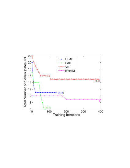
Figure 2: State Number Evolves over Iterations

Fig.2 shows how the hidden state numbers $K$ change over iterations in a typical trial. The final state numbers at convergence are shown at the end of each line. RFAB and FAB converge much faster than other methods ($<200$ iterations), which shows the shrinkage regularization accelerates the pruning of redundant states.

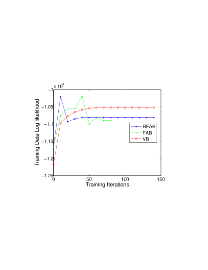
Figure 3: Training Data Log-likelihood

Fig.3 shows how training data log-likelihood changes over iterations in the same trial as in Fig.2. The log-likelihoods of RFAB and FAB on the training data are quite close. The log-likelihoods of iFHMM are not shown in this figure, as they are well below other methods (around -13500).

7 Conclusions and Future Work

The FHMM is a flexible and expressive model, but it also poses a difficult challenge on how to set its free, structural parameters. In this paper, we have successfully extended the recently-developed FAB framework onto the FHMM to address its model selection problem. We have derived a better asymptotic approximation of the data marginal likelihood than conventional FAB, by integrating out the initial and transition probabilities. Based on this refined marginal likelihood, an EM-like iterative optimization procedure, namely $\text{FAB}_{fhmm}$, has been developed, which can find both good model structures and model parameters at the same time. Experiments on a synthetic data set have shown that $\text{FAB}_{fhmm}$ obtains more parsimonious and better-fit models than the state-of-the-art nonparametric iFHMM and variational FHMM.

In addition, we have proved that, during the $\text{FAB}_{fhmm}$’s shrinkage process on hidden variables, if there are two very similar hidden states, then one state would almost surely “die out” and be pruned. This proof theoretically consolidates the shrinkage process which we observe in experiments.

Appendix A Appendix

Lemma 1.

Suppose $\{z_{n,1},\cdots,z_{n,T_{n}}\}_{n=1}^{N}$ are $N$ sequences of Bernoulli random variables, whose means are $\{p_{n,1},\cdots,p_{n,T_{n}}\}_{n=1}^{N}$. For the $n$-th sequence $\{z_{n,t}\}$, $z_{n,1},\cdots,z_{n,T_{n}}$ are independent with each other. Let $y_{n}=\sum_{i}z_{n,i}$, $\bar{y}_{n}=E[y_{n}]=\sum_{i}p_{n,i}$. Suppose further that $\bar{y}_{n}\to\infty$ as $T_{n}\to\infty$. Besides, there are $N$ numbers $\{\hat{y}_{n}\}$, $\forall n,\hat{y}_{n}\approx\bar{y}_{n}$. When all $T_{n}$ are large enough, the following bounds hold:

1)

$$\mathbf{E}[\log(y_{n}+1)] =\log(\hat{y}_{n}+1)+\frac{\bar{y}_{n}-\hat{y}_{n}}{\hat{y}_{n}+1}+\epsilon_{1};$$

2)

$$\mathbf{E}[y_{n}\log y_{n}]=\bar{y}_{n}\log\hat{y}_{n}+(\bar{y}_{n}-\hat{y}_{n})+\epsilon_{2}.$$

Here $\epsilon_{1},\epsilon_{2}$ are small bounded errors.

Proof.

1) Using the convexity of $-\log(y_{n}+1)$, we easily obtain

$$\mathbf{E}[\log(y_{n}+1)]\leq\log(\mathbf{E}[y_{n}]+1)=\log(\bar{y}_{n}+1).$$ (24)

We proceed to derive a lower bound of $\mathbf{E}[\log(y_{n}+1)]$.

The following lower bound of the logarithm function is well know:

$$\log x>1-\frac{1}{x}\quad\textnormal{for all }x>0.$$

Substituting $x$ with ${\displaystyle\frac{y_{n}+1}{\bar{y}_{n}+1}}$, we have

$$\log(y_{n}+1)-\log(\bar{y}_{n}+1)>1-\frac{\bar{y}_{n}+1}{y_{n}+1}.$$

After taking the expectation of both sides, it becomes

$$\mathbf{E}[\log(y_{n}+1)]-\log(\bar{y}_{n}+1)>1-(\bar{y}_{n}+1)\mathbf{E}\left[\frac{1}{y_{n}+1}\right].$$ (25)

$\mathbf{E}\left[\frac{1}{y_{n}+1}\right]$ is commonly referred to as the negative moment of $y_{n}$ [3]. We apply the corollary in [3] that

$$\mathbf{E}\left[\frac{1}{y_{n}+1}\right]=\int_{0}^{1}G_{n}(t)dt,$$ (26)

where $G_{n}(t)$ is the probability generating function of $y_{n}$. It is known that $G_{n}(t)=\prod_{i=1}^{T_{n}}(q_{n,i}+p_{n,i}\cdot t)$, in which $q_{n,i}=1-p_{n,i}$. Thus (26) becomes

$$\mathbf{E}\left[\frac{1}{y_{n}+1}\right]=\int_{0}^{1}\prod_{i=1}^{T_{n}}(q_{n,i}+p_{n,i}\cdot t)dt.$$ (27)

We apply the Inequality of arithmetic and geometric means to $\prod_{i=1}^{T_{n}}(q_{n,i}+p_{n,i}\cdot t)$:

$$\textnormal{$\forall$}t\geq 0:\quad\prod_{i=1}^{T_{n}}(q_{n,i}+p_{n,i}\cdot t) \leq\left(\frac{\sum_{i}q_{n,i}}{T_{n}}+\frac{\sum_{i}p_{n,i}}{T_{n}}t\right)^{T_{n}}$$

$$=(1-\frac{\bar{y}_{n}}{T_{n}}+\frac{\bar{y}_{n}}{T_{n}}t)^{T_{n}}.$$

Let $\bar{p}_{n}$ denote $\frac{\bar{y}_{n}}{T_{n}}$, and $\bar{q}_{n}$ denote $1-\frac{\bar{y}_{n}}{T_{n}}$. Then (27) becomes

$$\mathbf{E}\left[\frac{1}{y_{n}+1}\right]\leq\int_{0}^{1}(\bar{q}_{n}+\bar{p}_{n}t)^{T_{n}}dt=\frac{1-\bar{q}_{n}^{T_{n}+1}}{(T_{n}+1)\bar{p}_{n}}<\frac{1}{\bar{y}_{n}}.$$ (28)

Plugging (28) into (25), we have

$$\mathbf{E}[\log(y_{n}+1)]-\log(\bar{y}_{n}+1)>1-\frac{\bar{y}_{n}+1}{\bar{y}_{n}}=-\frac{1}{\bar{y}_{n}}.$$

Thus $-\frac{1}{\bar{y}_{n}}$ is the lower bound of the approximation error, which tends to 0 as $T_{n}\to\infty$. Hence

$$\exists\epsilon_{1a}>0,s.t.\;\forall T_{n},\mathbf{E}[\log(y_{n}+1)]>\log(\bar{y}_{n}+1)-\epsilon_{1a}.$$ (29)

Combining (24) and (29), we have

$$\big{|}\mathbf{E}[\log(y_{n}+1)]-\log(\bar{y}_{n}+1)\big{|}<\epsilon_{1a}.$$ (30)

On the other hand, as $\hat{y}_{n}\approx\bar{y}_{n}$, the first order approximation of $\log(\bar{y}_{n}+1)$ about $\hat{y}_{n}$ is good:

$$\log(\bar{y}_{n}+1)=\log(\hat{y}_{n}+1)+\frac{\bar{y}_{n}-\hat{y}_{n}}{\bar{y}_{n}+1}+\epsilon_{1b},$$ (31)

where $\epsilon_{1b}$ is an error of order $o(\bar{y}_{n}^{-1})$ that tends to 0 when $T_{n}$ increases.

Combining (30) and (31), we have

$$\left|\mathbf{E}[\log(y_{n}+1)]-\log(\hat{y}_{n}+1)-\frac{\bar{y}_{n}-\hat{y}_{n}}{\bar{y}_{n}+1}\right|<|\epsilon_{1a}|+|\epsilon_{1b}|.$$

In other words, $\log(\hat{y}_{n}+1)+\frac{\bar{y}_{n}-\hat{y}_{n}}{\bar{y}_{n}+1}$ approximates $\mathbf{E}[\log(y_{n}+1)]$ with a small bounded error. In addition, this error tends to 0 quickly as the sequence length $T_{n}$ increases.

2) It is easy to verify $y_{n}\log y_{n}$ is convex, and thus

$$\mathbf{E}[y_{n}\log y_{n}]\geq\bar{y}_{n}\log\bar{y}_{n}.$$ (32)

We proceed to derive an upper bound of $\mathbf{E}[y_{n}\log y_{n}]$.

Applying the inequality $\log x\leq x-1$ by substituting $x$ with $\frac{y_{n}}{\bar{y}_{n}}$, we have

$$y_{n}\log\frac{y_{n}}{\bar{y}_{n}}\leq y_{n}(\frac{y_{n}}{\bar{y}_{n}}-1)=\frac{y_{n}^{2}}{\bar{y}_{n}}-y_{n}.$$ (33)

Taking the expectation of both sides of (33), we have

$$\mathbf{E}[y_{n}\log y_{n}]-\bar{y}_{n}\log\bar{y}_{n}$$

$$\leq \frac{\mathbf{E}[y_{n}^{2}]}{\bar{y}_{n}}-\bar{y}_{n}$$

$$= \frac{\mathbf{Var}(y_{n})}{\bar{y}_{n}}$$

$$= \frac{\sum_{i}p_{n,i}^{2}}{\sum_{i}p_{n,i}}\leq 1.$$ (34)

Combining (32) and (34), we have

$$\mathbf{\text{$\big{|}$}E}[y_{n}\log y_{n}]-\bar{y}_{n}\log\bar{y}_{n}\big{|}\text{$\leq$1}.$$ (35)

Furthermore, when $\bar{y}_{n}\approx\hat{y}_{n}$, the first order approximation of $\log\bar{y}_{n}$ about $\hat{y}_{n}$ is good, i.e.:

$$\bar{y}_{n}(\log\bar{y}_{n}-\log\hat{y}_{n})$$

$$= \bar{y}_{n}(\bar{y}_{n}-\hat{y}_{n})/\hat{y}_{n}+\epsilon_{2a}$$

$$= (\bar{y}_{n}-\hat{y}_{n})+\frac{(\bar{y}_{n}-\hat{y}_{n})^{2}}{\hat{y}_{n}}+\epsilon_{2a},$$ (36)

where $\epsilon_{2a}$ is a small bounded error.

As $T_{n}\to\infty$ , both $\bar{y}_{n}$ and $\hat{y}_{n}$ tend to $\infty$. Therefore $\frac{(\bar{y}_{n}-\hat{y}_{n})^{2}}{\hat{y}_{n}}$ is a small bounded error $\epsilon_{2b}$. Then (36) becomes

$$\bar{y}_{n}\log\bar{y}_{n}-\bar{y}_{n}\log\hat{y}_{n}=(\bar{y}_{n}-\hat{y}_{n})+\epsilon_{2a}+\epsilon_{2b}.$$ (37)

Combining (35) and (37), we have

$$\mathbf{E}[y_{n}\log y_{n}]=\bar{y}_{n}\log\hat{y}_{n}+(\bar{y}_{n}-\hat{y}_{n})+\epsilon_{2},$$

where $|\epsilon_{2}|\leq|\epsilon_{2a}|+|\epsilon_{2b}|+1$ is also a small bounded error.

Corollary 2.

$\{y_{n}\}$, $\{\bar{y}_{n}\}$ and $\{\hat{y}_{n}\}$ are defined as the same as in Lemma 1. Then the following bounds hold:

1. $$\mathbf{E}[\log\Gamma(y_{n})]$$

   $$= \bar{y}_{n}(\log\hat{y}_{n}-\frac{1}{2\hat{y}_{n}})-(\hat{y}_{n}+\frac{1}{2}\log\hat{y}_{n})$$

   $$+\frac{1}{2}(\log 2\pi+1)+\epsilon_{3};$$

2. $$\mathbf{E}\left[\sum_{n}\!\log\!\Gamma(y_{n})\!-\!\log\!\Gamma(\sum_{n}y_{n})\right]$$

   $$= \sum_{n}\bar{y}_{n}\!\left[\log\!\big{(}\frac{\hat{y}_{n}}{\sum_{m}\hat{y}_{m}}\big{)}+\frac{1}{2\sum_{m}\hat{y}_{m}}-\frac{1}{2\hat{y}_{n}}\right]$$

   $$+\frac{1}{2}\log\big{(}\sum_{n}\hat{y}_{n}\big{)}-\frac{1}{2}\sum_{n}\log\hat{y}_{n}$$

   $$+\frac{1}{2}(N-1)(\log 2\pi+1)+\epsilon_{4}.$$

Here $\epsilon_{3},\epsilon_{4}$ are small bounded errors.

Proof.

1) The Stirling’s approximation for the log-Gamma function is:

$$\log\Gamma(y_{n})=(y_{n}-\frac{1}{2})\log y_{n}-y_{n}+\frac{1}{2}\log 2\pi+\epsilon_{3a},$$ (38)

where $\epsilon_{3a}$ is an error term of $O(y^{-1})$, which goes to zero quickly as $T_{n}$ increases. Therefore $\mathbf{E}[\epsilon_{3a}]$, denoted as $\bar{\epsilon}_{3a}$, is also a small bounded number.

Taking the expectation of both sides of (38), and applying Lemma 1, we obtain

$$\mathbf{E}[\log\Gamma(y_{n})]$$

$$= \bar{y}_{n}(\log\hat{y}_{n}-\frac{1}{2\hat{y}_{n}})-(\hat{y}_{n}+\frac{1}{2}\log\hat{y}_{n})+\frac{1}{2}(\log 2\pi+1)+\epsilon_{3}.$$

2) Obtained by repeatedly applying 1), and combining terms involving $\bar{y}_{n}$.

References

• [1] M. Beal. Variational algorithms for approximate Bayesian inference. PhD thesis, University of London, 2003.
• [2] G. Celeux and J.-B. Durand. Selecting hidden markov model state number with cross-validated likelihood. Computational Statistics, 23:541–564, 2008.
• [3] M. T. Chao and W. E. Strawderman. Negative moments of positive random variables. Journal of the American Statistical Association, 67(338):429–431, 1972.
• [4] K. Duh. Jointly labeling multiple sequences: a factorial hmm approach. In Proceedings of the ACL Student Research Workshop, ACLstudent ’05, pages 19–24, Stroudsburg, PA, USA, 2005. Association for Computational Linguistics.
• [5] R. Eto, R. Fujimaki, S. Morinaga, and T. Hiroshi. Fully-automatic bayesian piece-wise sparse linear models. In Proceedings of the 17th International Conference on Artificial Intelligence and Statistics (AISTATS), 2014.
• [6] R. Fujimaki and K. Hayashi. Factorized asymptotic bayesian hidden markov models. In ICML, volume 22, pages 400–408, 2012.
• [7] R. Fujimaki and S. Morinaga. Factorized asymptotic bayesian inference for mixture modeling. In AISTATS, volume 22, pages 400–408, 2012.
• [8] Z. Ghahramani and M. I. Jordan. Factorial hidden markov models. Machine Learning, 29:245–273, 1997. 10.1023/A:1007425814087.
• [9] K. Hayashi and R. Fujimaki. Factorized asymptotic bayesian inference for latent feature models. In 27th Annual Conference on Neural Information Processing Systems (NIPS), 2013.
• [10] D. Husmeier. Discriminating between rate heterogeneity and interspecific recombination in dna sequence alignments with phylogenetic factorial hidden markov models. Bioinformatics, 21(suppl 2):ii166–ii172, 2005.
• [11] H. Kim, M. Marwah, M. F. Arlitt, G. Lyon, and J. Han. Unsupervised disaggregation of low frequency power measurements. In SDM, pages 747–758, 2011.
• [12] J. Z. Kolter and T. Jaakkola. Approximate inference in additive factorial hmms with application to energy disaggregation. In AISTATS, volume 22, pages 1472–1482, 2012.
• [13] B. Leroux. Maximum-likelihood estimation for hidden markov models. Stochastic processes and their applications, 40(1):127–143, 1992.
• [14] C. A. McGrory and D. M. Titterington. Variational bayesian analysis for hidden markov models. Australian & New Zealand Journal of Statistics, 51(2):227–244, 2009.
• [15] G. Mysore and M. Sahani. Variational inference in non-negative factorial hidden markov models for efficient audio source separation. In ICML, 2012.
• [16] A. V. Nefian, L. Liang, X. Pi, X. Liu, and K. Murphy. Dynamic bayesian networks for audio-visual speech recognition. EURASIP Journal on Advances in Signal Processing, 2002(11):1274–1288, 2002.
• [17] L. Rabiner. A tutorial on hidden markov models and selected applications in speech recognition. Proceedings of the IEEE, 77(2):257–286, 1989.
• [18] S. T. Roweis et al. One microphone source separation. In Advances in neural information processing systems, pages 793–799. MIT; 1998, 2001.
• [19] J. Van Gael, Y. W. Teh, and Z. Ghahramani. The infinite factorial hidden markov model. In Neural Information Processing Systems, volume 21, 2008.