A Comprehensive Survey of Potential Game Approaches to Wireless Networks

Abstract

Potential games form a class of non-cooperative games where unilateral improvement dynamics are guaranteed to converge in many practical cases. The potential game approach has been applied to a wide range of wireless network problems, particularly to a variety of channel assignment problems. In this paper, the properties of potential games are introduced, and games in wireless networks that have been proven to be potential games are comprehensively discussed.

I Introduction

The broadcast nature of wireless transmissions causes co-channel interference and channel contention, which can be viewed as interactions among transceivers. Interactions among multiple decision makers can be formulated and analyzed using a branch of applied mathematics called game theory [131, 61]. Game-theoretic approaches have been applied to a wide range of wireless communication technologies, including transmission power control for code division multiple access (CDMA) cellular systems [153] and cognitive radios [132]. For a summary of game-theoretic approaches to wireless networks, we refer the interested reader to [108, 92, 68, 168, 91]. Application-specific surveys of cognitive radios and sensor networks can be found in [178, 102, 187, 160, 64, 166].

In this paper, we focus on potential games [126], which form a class of strategic form games with the following desirable properties:

• The existence of a Nash equilibrium in potential games is guaranteed in many practical situations [126] (Theorems 1 and 2 in this paper), but is not guaranteed for general strategic form games. Other classes of games possessing Nash equilibria are summarized in [92, §2.2] and [68, §3.4].

• Unilateral improvement dynamics in potential games with finite strategy sets are guaranteed to converge to the Nash equilibrium in a finite number of steps, i.e., they do not cycle [126] (Theorem 4 in this paper). As a result, learning algorithms can be systematically designed.

A game that does not have these properties is discussed in Example 2 in Section II.

We provide an overview of problems in wireless networks that can be formulated in terms of potential games. We also clarify the relations among games, and provide simpler proofs of some known results. Problem-specific learning algorithms [92, 168] are beyond the scope of this paper.

TABLE I: Games discussed in this paper.

Section	System model	Strategy	Payoff
V	Fig. 1LABEL:sub@fig:model2	Channel	Interference power
VI	Fig. 1LABEL:sub@fig:model2	Channel	SINR or Shannon capacity
VII	Fig. 1LABEL:sub@fig:model2	Channel	Number of interference signals
VIII	Figs. 1LABEL:sub@fig:model3 and 1LABEL:sub@fig:model4	Channel	Interference power
IX	Figs. 1LABEL:sub@fig:model3 and 1LABEL:sub@fig:model4	Channel	SINR or Shannon capacity
X	Fig. 1LABEL:sub@fig:model5	Channel	Number of interference signals
XI	Fig. 1LABEL:sub@fig:model5	Channel	Successful access probability or throughput
XII	Fig. 1LABEL:sub@fig:model5	Transmission probability	Successful access probability or throughput
XIII	Fig. 1LABEL:sub@fig:model1	Transmission power	Throughput or Shannon capacity
XIV	Fig. 1LABEL:sub@fig:model3	Transmission power	Connectivity
XV	Fluid network	Amount of traffic	Congestion cost
XVI	M/M/1 queue	Arrival rate	Trade-off between throughput and delay
XVII	Mobile sensors	Location	Connectivity or coverage
XVIII	Immobile sensors	Channel	Coverage

The remainder of this paper is organized as follows: In Sections II, III, and IV, we introduce strategic form games, potential games, and learning algorithms, respectively. We then discuss various potential games in Sections V to XVIII, as shown in Table I. Finally, we provide a few concluding remarks in Section XIX.

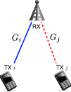
(a) Multiple-access channel.

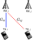
(b) TX-RX pairs ($G_{ij}\neq G_{ji}$).

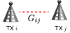
(c) TXs ($G_{ij}=G_{ji}$).

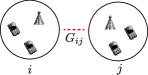
(d) Canonical network model ($G_{ij}=G_{ji}$).

(e) Interference graph.

Figure 1: System models. Straight blue lines represent communication channels of player $i$ and red dashed lines represent interference channels to player $i$.

The notation used here is shown in Table II. Unless the context indicates otherwise, sets of strategies are denoted by calligraphic uppercase letters, e.g., $\mathcal{A}_{i}$, strategies are denoted by lowercase letters, e.g., $a_{i}\in\mathcal{A}_{i}$, and tuples of strategies are denoted by boldface lowercase letters, e.g., $\boldsymbol{a}$. Note that $a_{i}$ is a scalar variable when $\mathcal{A}_{i}$ is a set of scalars or indices, $a_{i}$ is a vector variable when $\mathcal{A}_{i}$ is a set of vectors, and $a_{i}$ is a set variable when $\mathcal{A}_{i}$ is a collection of sets.

We use $\mathbb{R}$ to denote the set of real numbers, $\mathbb{R}_{+}$ to denote the set of nonnegative real numbers, $\mathbb{R}_{++}$ to denote the set of positive real numbers, and $\mathbb{C}$ to denote the set of complex numbers. The cardinality of set $\mathcal{A}$ is denoted by $\lvert\mathcal{A}\rvert$. The power set of $\mathcal{A}$ is denoted by $2^{\mathcal{A}}$. Finally, $\mathop{\mathbbm{1}}\nolimits_{{\mathit{condition}}}$ is the indicator function, which is one when $\mathit{condition}$ is true and is zero otherwise.

We treat many system models, as shown in Fig. 1. In multiple-access channels, as shown in Fig. 1LABEL:sub@fig:model1, multiple transmitters (TXs/users/mobile stations/terminals) transmit signals to a single receiver (RX/base station (BS)/access point (AP)). In Fig. 1LABEL:sub@fig:model1, $G_{i}$ represents the link gain from TX $i$ to the RX.

In a network model consisting of TX-RX pairs, as shown in Fig. 1LABEL:sub@fig:model2, each TX $i$ transmits signals to RX $i$. In this case, $G_{ij}\neq G_{ji}$. In a network model consisting of TXs shown in Fig. 1LABEL:sub@fig:model3, each TX (BS/AP/transceiver/station/terminal/node) interferes with others. In this model, $G_{ij}=G_{ji}$. A “canonical network model” [15], shown in Fig. 1LABEL:sub@fig:model4, consists of clusters that are spatially separated in order for $G_{ij}=G_{ji}$ to hold. Note that these network models have been discussed in terms of graph structure in [143].

We use $ji$ to denote a directed link from TX $i$ to TX $j$ or cluster $i$ to cluster $j$. Let interference graph $(\mathcal{I},\mathcal{E})$ be an undirected graph, where the set of vertices $\mathcal{I}=\{1,2,\dots\}$ corresponds to TXs or clusters, and $i$ interferes with $j$ if $ji\in\mathcal{E}$, as shown in Fig. 1LABEL:sub@fig:model5, i.e., $\mathcal{E}\coloneqq\{\,ji\mid G_{ji}P>T\,\}$ where $P$ is the transmission power level for every TX and $T$ is a threshold of the received power. Note that in undirected graph $(\mathcal{I},\mathcal{E})$, $ji\in\mathcal{E}\Leftrightarrow ij\in\mathcal{E}$, for every $\{i,j\}\subset\mathcal{I}$. We denote the neighborhood of $i$ in graph $(\mathcal{I},\mathcal{E})$ by $\mathcal{I}_{i}\coloneqq\{\,j\in\mathcal{I}\setminus\{i\}\mid ji\in\mathcal{E}\,\}$. We also define $\mathcal{I}_{i}^{c_{i}}(\boldsymbol{c})\coloneqq\{\,j\in\mathcal{I}_{i}\mid c_{j}=c_{i}\,\}$, then, $\lvert\mathcal{I}_{i}^{c_{i}}(\boldsymbol{c})\rvert=\sum_{j\in\mathcal{I}_{i}}\mathop{\mathbbm{1}}\nolimits_{{c_{j}=c_{i}}}=\sum_{j\neq i}\mathop{\mathbbm{1}}\nolimits_{{c_{j}=c_{i}}}\mathop{\mathbbm{1}}\nolimits_{{ij\in\mathcal{E}}}$.

TABLE II: Notation.

$\mathcal{G}$	Strategic form game
$\mathcal{I}$	Finite set of players, $\mathcal{I}=\{1,2,\dots,\lvert\mathcal{I}\rvert\}$
$\mathcal{I}^{f}(\boldsymbol{a})$	$\coloneqq\{\,i\in\mathcal{I}\mid f\in a_{i}\,\}$
$\mathcal{A}_{i}$	Set of strategies for player $i\in\mathcal{I}$
$\mathcal{A}$	Strategy space, $\prod_{i\in\mathcal{I}}\mathcal{A}_{i}$
$u_{i}$	Payoff function for player $i\in\mathcal{I}$
$\phi$	Potential function
$\mathop{\mathrm{BR}}\nolimits_{i}$	Best-response correspondence of player $i$
$a_{i}$	Strategy of player $i$, $a_{i}\in\mathcal{A}_{i}$
$\Delta(\mathcal{A}_{i})$	Set of probability distributions over $\mathcal{A}_{i}$
$x_{i}$	Mixed strategy, $x_{i}\in\Delta(\mathcal{A}_{i})$
$\boldsymbol{x}$	Mixed strategy profile, $\boldsymbol{x}\in\prod_{i}\Delta(\mathcal{A}_{i})$
$G_{i}$	Link gain between TX $i$ and a single isolated RX in Fig. 1LABEL:sub@fig:model1
$G_{ij}$	Link gain between TX $j$ and RX $i$; $G_{ji}\neq G_{ij}$ in Fig. 1LABEL:sub@fig:model2, and $G_{ji}=G_{ij}$ in Figs. 1LABEL:sub@fig:model3 and 1LABEL:sub@fig:model4
$ji$	Directed link from $i$ to $j$
$\mathcal{E}$	Set of edges in undirected graph
$\mathcal{I}_{i}$	$\coloneqq\{\,j\in\mathcal{I}\setminus\{i\}\mid ji\in\mathcal{E}\,\}$. Neighborhood in graph $(\mathcal{I},\mathcal{E})$
$\mathcal{I}_{i}^{c_{i}}(\boldsymbol{c})$	$\coloneqq\{\,j\in\mathcal{I}_{i}\mid c_{j}=c_{i}\,\}$.
$N$	Common noise power for every player
$N_{i}$	Noise power at RX $i$
$N_{i}(c_{i})$	Noise power at RX $i$ in channel $c_{i}$
$I_{i}(\boldsymbol{c})$	Interference power at RX $i$ at channel arrangement $\boldsymbol{c}$
$\mathcal{C}_{i}$	Set of available channels for player $i$
$c_{i}\ (\in\mathcal{C}_{i})$	Channel of player $i$
$\boldsymbol{c}$	$\coloneqq(c_{i})_{i\in\mathcal{I}}\in\prod_{i}\mathcal{C}_{i}$
$\mathcal{P}_{i}$	Set of available transmission power levels for player $i$
$p_{i}\ (\in\mathcal{P}_{i})$	Transmission power level of player $i$ as a strategy
$\boldsymbol{p}$	$\coloneqq(p_{i})_{i\in\mathcal{I}}\in\prod_{i}\mathcal{P}_{i}$
$P$	Identical transmission power level for every player
$P_{i}$	Transmission power level for player $i$ as a constant
$\varGamma$	Required signal-to-interference-plus-noise power ratio (SINR)

II Game-theoretic Framework

We begin with the definition of a strategic form game and present an example of a game-theoretic formulation of a simple channel selection problem. Moreover, we discuss other useful concepts, such as the best response and Nash equilibrium. The analysis of Nash equilibria in the channel selection example reveals the potential presence of cycles in best-response adjustments.

Definition 1

A strategic (or normal) form game is a triplet $\mathcal{G}\coloneqq(\mathcal{I},(\mathcal{A}_{i})_{i\in\mathcal{I}},(u_{i})_{i\in\mathcal{I}})$, or simply $\mathcal{G}\coloneqq(\mathcal{I},(\mathcal{A}_{i}),(u_{i}))$, where $\mathcal{I}=\{1,2,\dots,\lvert\mathcal{I}\rvert\}$ is a finite set of players (decision makers), $\mathcal{A}_{i}$ is the set of strategies (or actions) for player $i\in\mathcal{I}$, and $u_{i}\colon\prod_{i\in\mathcal{I}}\mathcal{A}_{i}\to\mathbb{R}$ is the payoff (or utility) function of player $i\in\mathcal{I}$ that must be maximized.

If $\mathcal{S}\subseteq\mathcal{I}$, we denote the Cartesian product $\prod_{i\in\mathcal{S}}\mathcal{A}_{i}$ by $\mathcal{A}_{\mathcal{S}}$. If $\mathcal{S}=\mathcal{I}$, we simply write $\mathcal{A}$ to denote $\mathcal{A}_{\mathcal{I}}$, and $\sum_{i}$ to denote $\sum_{i\in\mathcal{I}}$. When $\mathcal{S}=\mathcal{I}\setminus\{i\}$, we let $\mathcal{A}_{-i}$ denote $\mathcal{A}_{\mathcal{I}\setminus\{i\}},$ and $\sum_{j\neq i}$ denote $\sum_{j\in\mathcal{I}\setminus\{i\}}$. For $a_{i}\in\mathcal{A}_{i}$, $\boldsymbol{a}_{\mathcal{S}}=(a_{i})_{i\in\mathcal{S}}\in\mathcal{A}_{\mathcal{S}}$, $\boldsymbol{a}=(a_{i},\boldsymbol{a}_{-i})=(a_{1},\ldots,a_{\lvert\mathcal{I}\rvert})\in\mathcal{A}$, and $\boldsymbol{a}_{-i}=(a_{1},\ldots,a_{i-1},a_{i+1},\ldots,a_{\lvert\mathcal{I}\rvert})\in\mathcal{A}_{-i}$.

Example 1

Consider a channel selection problem in the TX-RX pair model shown in Fig. 1LABEL:sub@fig:model2. Each TX-RX pair is assumed to select its channel in a decentralized manner in order to minimize the received interference power.

The channel selection problem can be formulated as a strategic form game $\mathcal{G}1\coloneqq(\mathcal{I},(\mathcal{C}_{i}),(u{\ref{g:u1}}_{i}))$. The elements of the game are as follows: the set of players $\mathcal{I}$ is the set of TX-RX pairs. The strategy set for each pair $i$, $\mathcal{C}_{i}$ is the set of available channels. The received interference power at RX $i\in\mathcal{I}$ is determined by a combination of channels $\boldsymbol{c}=(c_{i})_{i\in\mathcal{I}}\in\mathcal{C}=\prod_{i}\mathcal{C}_{i}$, where

$$I_{i}(\boldsymbol{c}) \coloneqq\sum_{j\neq i}G_{ij}P\mathop{\mathbbm{1}}\nolimits_{{c_{j}=c_{i}}}.$$ (1)

Let $-I_{i}(\boldsymbol{c})$ be the payoff function to be maximized, i.e.,

$$u{\ref{g:u1}}_{i}(\boldsymbol{c})\coloneqq-I_{i}(\boldsymbol{c})=-\sum_{j\neq i}G_{ij}P\mathop{\mathbbm{1}}\nolimits_{{c_{j}=c_{i}}}.$$ (2)

Note that $\mathcal{G}{\ref{g:u1}}$ was introduced in [140], and we further discuss it in Example 2.

Definition 2

The best-response correspondence (or simply, best response) $\mathop{\mathrm{BR}}\nolimits_{i}\colon\mathcal{A}_{-i}\to 2^{\mathcal{A}_{i}}$ of player $i$ to strategy profile $\boldsymbol{a}_{-i}$ is the correspondence

$$\mathop{\mathrm{BR}}\nolimits_{i}(\boldsymbol{a}_{-i})\\ \coloneqq\{\,a_{i}\in\mathcal{A}_{i}\mid u_{i}(a_{i},\boldsymbol{a}_{-i})\geq u_{i}(a_{i}^{\prime},\boldsymbol{a}_{-i}),\forall a_{i}^{\prime}\in\mathcal{A}_{i}\,\},$$ (3)

or equivalently, $\mathop{\mathrm{BR}}\nolimits_{i}(\boldsymbol{a}_{-i})\coloneqq\arg\max_{a_{i}\in\mathcal{A}_{i}}u_{i}(a_{i},\boldsymbol{a}_{-i})$.

A fundamental solution concept for strategic form games is the Nash equilibrium:

Definition 3

A strategy profile $\boldsymbol{a}^{*}=(a_{i}^{*},\boldsymbol{a}_{-i}^{*})\in\mathcal{A}$ is a pure-strategy Nash equilibrium (or simply a Nash equilibrium) of game $(\mathcal{I},(\mathcal{A}_{i}),(u_{i}))$ if

$$u_{i}(a_{i}^{*},\boldsymbol{a}_{-i}^{*})\geq u_{i}(a_{i},\boldsymbol{a}_{-i}^{*}),$$ (4)

for every $i\in\mathcal{I}$ and $a_{i}\in\mathcal{A}_{i}$; equivalently, $a_{i}^{*}\in\mathop{\mathrm{BR}}\nolimits_{i}(\boldsymbol{a}_{-i}^{*})$ for every $i\in\mathcal{I}$. That is, $a_{i}^{*}$ is a solution to the optimization problem $\max_{a_{i}\in\mathcal{A}_{i}}u_{i}(a_{i},\boldsymbol{a}_{-i}^{*})$.

At the Nash equilibrium, no player can improve his/her payoff by adopting a different strategy unilaterally; thus, no player has an incentive to unilaterally deviate from the equilibrium. The Nash equilibrium is a proper solution concept; however, the existence of a pure-strategy Nash equilibrium is not necessarily guaranteed, as shown in the next example.

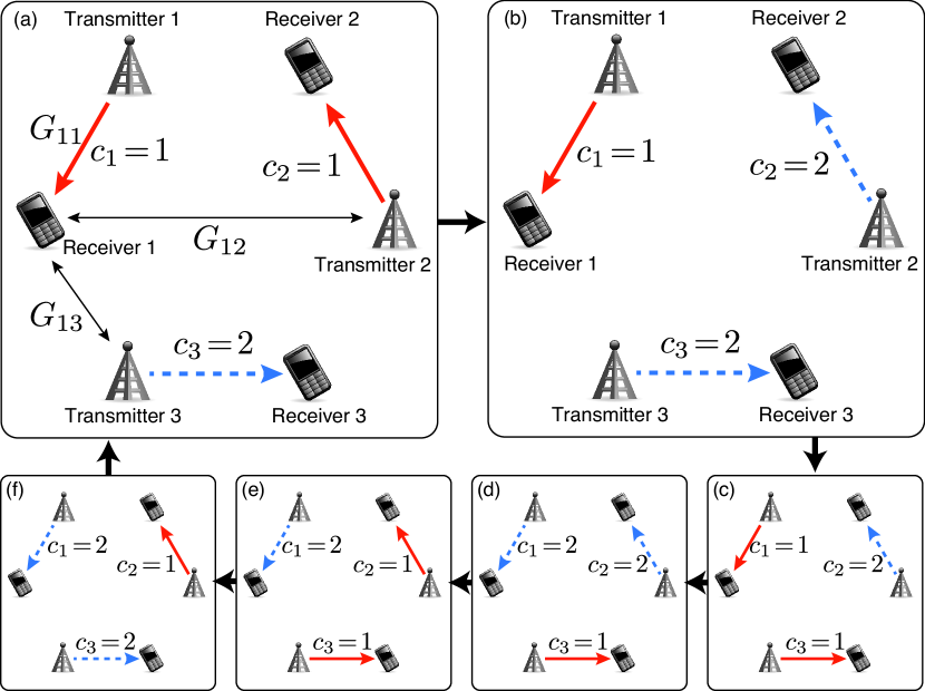
Figure 2: Arrangement used in Example 2. A cycle results from the best-response adjustment.

Example 2

Consider $\mathcal{G}{\ref{g:u1}}$ and the arrangement shown in Fig. 2, i.e., $\mathcal{I}=\{1,2,3\}$, $\mathcal{C}_{i}=\{1,2\}$ for every $i$, and $G_{13}>G_{12}$, $G_{21}>G_{23}$, and $G_{32}>G_{31}$. The game does not have a Nash equilibrium, i.e., for every channel allocation, at least one pair has an incentive to change his/her channel. The details are as follows: when all players choose the same channel, e.g., $(c_{1},c_{2},c_{3})=(1,1,1)$, every player has an incentive to change his/her channel because $\mathop{\mathrm{BR}}\nolimits_{i}(\boldsymbol{c}_{-i})=\{2\}$ for all $i$; thus, it is not in Nash equilibrium. On the contrary, when two players choose the same channel, and the third player chooses a different channel, e.g., $(c_{1},c_{2},c_{3})=(1,1,2)$, as shown in Fig. 2(a), $\mathop{\mathrm{BR}}\nolimits_{2}(\boldsymbol{c}_{-2})=\{2\}$, i.e., pair 2 has an incentive to change its channel $a_{2}$ from 1 to 2, and (4) does not hold. Because of the symmetry property of the arrangement in Fig. 2, every strategy profile does not satisfy (4). Furthermore, the best-response channel adjustments, which will be formally discussed in Section IV, cycle as $(1,1,2)$, $(1,2,2)$, $(1,2,1)$, $(2,2,1)$, $(2,1,1)$, $(2,1,2)$, and $(1,1,2)$, as shown in Figs. 2(a-f).

The channel allocation game $\mathcal{G}{\ref{g:u1}}$ is discussed further in Section V.

III Potential Games

We state key definitions and properties of potential games in Section III-A, show how to identify and design exact potential games in Sections III-B and III-C, and show how to identify ordinal potential games in Section III-D.

III-A Definitions and Properties of Potential Games

Monderer and Shapley [126] introduced the following classes of potential games:

Definition 4

A strategic form game $(\mathcal{I},(\mathcal{A}_{i}),(u_{i}))$ is an exact potential game (EPG) if there exists an exact potential function $\phi\colon\mathcal{A}\to\mathbb{R}$ such that

$$u_{i}(a_{i},\boldsymbol{a}_{-i})-u_{i}(a_{i}^{\prime},\boldsymbol{a}_{-i}) =\phi(a_{i},\boldsymbol{a}_{-i})-\phi(a_{i}^{\prime},\boldsymbol{a}_{-i}),$$ (5)

for every $i\in\mathcal{I}$, $a_{i},a_{i}^{\prime}\in\mathcal{A}_{i}$, and $\boldsymbol{a}_{-i}\in\mathcal{A}_{-i}$.

Definition 5

A strategic form game $(\mathcal{I},(\mathcal{A}_{i}),(u_{i}))$ is a weighted potential game (WPG) if there exist a weighted potential function $\phi\colon\mathcal{A}\to\mathbb{R}$ and a set of positive numbers $\{\alpha_{i}\}_{i\in\mathcal{I}}$ such that

$$u_{i}(a_{i},\boldsymbol{a}_{-i})-u_{i}(a_{i}^{\prime},\boldsymbol{a}_{-i})=\alpha_{i}(\phi(a_{i},\boldsymbol{a}_{-i})-\phi(a_{i}^{\prime},\boldsymbol{a}_{-i})),$$ (6)

for every $i\in\mathcal{I}$, $a_{i},a_{i}^{\prime}\in\mathcal{A}_{i}$, and $\boldsymbol{a}_{-i}\in\mathcal{A}_{-i}$.

Definition 6

A strategic form game $(\mathcal{I},(\mathcal{A}_{i}),(u_{i}))$ is an ordinal potential game (OPG) if there exists an ordinal potential function $\phi\colon\mathcal{A}\to\mathbb{R}$ such that

$$\mathop{\mathrm{sgn}}\nolimits(u_{i}(a_{i},\boldsymbol{a}_{-i})-u_{i}(a_{i}^{\prime},\boldsymbol{a}_{-i}))\\ =\mathop{\mathrm{sgn}}\nolimits(\phi(a_{i},\boldsymbol{a}_{-i})-\phi(a_{i}^{\prime},\boldsymbol{a}_{-i})),$$ (7)

for every $i\in\mathcal{I}$, $a_{i},a_{i}^{\prime}\in\mathcal{A}_{i}$, and $\boldsymbol{a}_{-i}\in\mathcal{A}_{-i}$, where $\mathop{\mathrm{sgn}}\nolimits(\cdot)$ denotes the sign function.

Although the potential function $\phi$ is independent of the indices of the players, $\phi$ reflects any unilateral change in any payoff function $u_{i}$ for every player $i$.

Since an EPG is a WPG and a WPG is an OPG [126, 177], the following properties of OPGs are satisfied by EPGs and WPGs.

Theorem 1 (Existence in finite OPGs)

Every OPG with finite strategy sets possesses at least one Nash equilibrium [126, Corollary 2.2].

Theorem 2 (Existence in infinite OPGs)

In the case of infinite strategy sets, every OPG with compact strategy sets and continuous payoff functions possesses at least one Nash equilibrium [126, Lemma 4.3].

Theorem 3 (Uniqueness)

Every OPG with a compact and convex strategy space, and a strictly concave and continuously differentiable potential function possesses a unique Nash equilibrium [138, Theorem 2], [154].

The most important property of potential games is acyclicity, which is also referred to as the finite improvement property.

Definition 7 (Finite improvement property [126])

A path in $(\mathcal{I},(\mathcal{A}_{i}),(u_{i}))$ is a sequence $(\boldsymbol{a}[0],\boldsymbol{a}[1],\ldots)$ such that for every integer $k\geq 1$, there exists a unique player $i$ such that $a_{i}[k]\neq a_{i}[k\!-\!1]\in\mathcal{A}_{i}$ while $\boldsymbol{a}_{-i}[k]=\boldsymbol{a}_{-i}[k\!-\!1]$. $(\boldsymbol{a}[0],\boldsymbol{a}[1],\ldots)$ is an improvement path if, for every $k\geq 1$, $u_{i}(\boldsymbol{a}[k])>u_{i}(\boldsymbol{a}[k\!-\!1])$, where $i$ is the unique deviator at step $k$. $(\mathcal{I},(\mathcal{A}_{i}),(u_{i}))$ has the finite improvement property (FIP) if every improvement path is finite.

Theorem 4

Every OPG with finite strategy sets has the FIP [126, Lemma 2.3]; that is, unilateral improvement dynamics are guaranteed to converge to a Nash equilibrium in a finite number of steps.

III-B Identification of Exact Potential Games

The definition of an EPG utilizes a potential function (5). Sometimes, however, it is beneficial to know if a given game is an EPG independently of its potential function. The following properties of EPGs and classes of games known to be EPGs are useful for the identification and derivation of potential functions. Note that each EPG has a unique exact potential function except for an additive constant [126, Lemma 2.7].

Theorem 5

Let $(\mathcal{I},(\mathcal{A}_{i}),(u_{i}))$ be a strategic form game where strategy sets $\mathcal{A}_{i}$ are intervals of real numbers and payoff functions $u_{i}$ are twice continuously differentiable. Then, the game is an EPG if and only if

$$\frac{\partial^{2}u_{i}(\boldsymbol{a})}{\partial a_{i}\,\partial a_{j}} =\frac{\partial^{2}u_{j}(\boldsymbol{a})}{\partial a_{i}\,\partial a_{j}},$$ (8)

for every $i,j\in\mathcal{I}$ [126, Theorem 4.5].

Theorem 6

Let $(\mathcal{I},(\mathcal{A}_{i}),(u_{i,1}))$ and $(\mathcal{I},(\mathcal{A}_{i}),(u_{i,2}))$ be EPGs with potential functions $\phi_{1}(\boldsymbol{a})$ and $\phi_{2}(\boldsymbol{a})$, respectively. Furthermore, let $\alpha,\ \beta\in\mathbb{R}$. Then, $(\mathcal{I},(\mathcal{A}_{i}),(\alpha u_{i,1}+\beta u_{i,2}))$ is an EPG with potential function $\alpha\phi_{1}(\boldsymbol{a})+\beta\phi_{2}(\boldsymbol{a})$ [59].

III-B1 Coordination-dummy Games

If $u_{i}(\boldsymbol{a})=u(\boldsymbol{a})$ for all $i\in\mathcal{I}$, where $u\colon\mathcal{A}\to\mathbb{R}$, the game $(\mathcal{I},(\mathcal{A}_{i}),(u))$ is called a coordination game or an identical interest game, and $u$ is called a coordination function [59].

If $u_{i}(\boldsymbol{a})=d_{i}(\boldsymbol{a}_{-i})$ for all $i\in\mathcal{I}$, where $d_{i}\colon\mathcal{A}_{-i}\to\mathbb{R}$, the game $(\mathcal{I},(\mathcal{A}_{i}),(d_{i}))$ is called a dummy game, and $d_{i}$ is called a dummy function [59].

If $u_{i}(\boldsymbol{a})=s_{i}(a_{i})$ for all $i\in\mathcal{I}$, where $s_{i}\colon\mathcal{A}_{i}\to\mathbb{R}$, the game $(\mathcal{I},(\mathcal{A}_{i}),(s_{i}))$ is called a self-motivated game, and $s_{i}$ is called a self-motivated function [133].

Theorem 7

$(\mathcal{I},(\mathcal{A}_{i}),(u_{i}))$ is an EPG if and only if there exist functions $u\colon\mathcal{A}\to\mathbb{R}$ and $d_{i}\colon\mathcal{A}_{-i}\to\mathbb{R}$ such that

$$u_{i}(a_{i},\boldsymbol{a}_{-i})=u(a_{i},\boldsymbol{a}_{-i})+d_{i}(\boldsymbol{a}_{-i}),$$ (9)

for every $i\in\mathcal{I}$ [163, 59]. This game is said to be a coordination-dummy game. The potential function of this game is $\phi(\boldsymbol{a})=u(\boldsymbol{a})$.

Example 3

From Theorem 7, any identical interest game is an EPG. Almost all games found in studies applying identical interest games [165, 74, 107, 55, 27, 142, 19] have the form of game $\mathcal{G}2\coloneqq(\mathcal{I},(\mathcal{A}_{i}),(u{\ref{g:coord}}_{i}))$, where

$$u{\ref{g:coord}}_{i}(\boldsymbol{a}) \coloneqq\sum_{j}f_{j}(\boldsymbol{a}),$$ (10)

for every $i\in\mathcal{I}$ and $f_{j}(\boldsymbol{a})$ is a performance indicator of player $j$, e.g., $f_{j}(\boldsymbol{a})$ is the individual throughput and $u{\ref{g:coord}}_{i}(\boldsymbol{a})$ is the aggregated throughput of all players [165]. Note that in most of these works, $\mathcal{G}{\ref{g:coord}}$ is used for comparison with other games.

Example 4

Closely related to $\mathcal{G}{\ref{g:coord}}$, the form of game $\mathcal{G}3$ with payoff

$$u{\ref{eq:coord_graph}}_{i}(\boldsymbol{a}) \coloneqq f_{i}(a_{i},\boldsymbol{a}_{\mathcal{I}_{i}})+\sum_{j\in\mathcal{I}_{i}}f_{j}(a_{j},\boldsymbol{a}_{\mathcal{I}_{j}}),$$ (11)

where $f_{i}\colon\mathcal{A}_{i}\times\mathcal{A}_{\mathcal{I}_{i}}\to\mathbb{R}$, is found in many scenarios: data stream control in multiple-input and multiple-output (MIMO) [14], channel assignment [188], joint power, channel and BS assignment [162], joint power and user scheduling [206], BS selection [54], and BS sleeping [208]. Note that $\mathcal{G}{\ref{eq:coord_graph}}$ is not an identical interest game, but can be seen as $\mathcal{G}{\ref{g:coord}}$ on graphs, where the performance indicator of player $i$ is a function of strategies of its neighbors, i.e., $f_{i}\colon\mathcal{A}_{i}\times\mathcal{A}_{\mathcal{I}_{i}}\to\mathbb{R}$, and the sum of the performance indicators of player $i$ and neighbors $\mathcal{I}_{i}$ is set for the payoff function of player $i$. It can be easily proved that $\mathcal{G}{\ref{eq:coord_graph}}$ is an EPG with potential

$$\phi{\ref{eq:coord_graph}}(\boldsymbol{a}) =\sum_{i}f_{i}(a_{i},\boldsymbol{a}_{\mathcal{I}_{i}}).$$ (12)

III-B2 Bilateral Symmetric Interaction Games

A strategic form game $\mathcal{G}4\coloneqq(\mathcal{I},(\mathcal{A}_{i}),(u{\ref{eq:bsi}}_{i}))$ is called a bilateral symmetric interaction (BSI) game if there exist functions $w_{ij}\colon\mathcal{A}_{i}\times\mathcal{A}_{j}\to\mathbb{R}$ and $s_{i}\colon\mathcal{A}_{i}\to\mathbb{R}$ such that

$$u{\ref{eq:bsi}}_{i}(\boldsymbol{a}) =\sum_{j\neq i}w_{ij}(a_{i},a_{j})-s_{i}(a_{i}),$$ (13)

where $w_{ij}(a_{i},a_{j})=w_{ji}(a_{j},a_{i})$ for every $(a_{i},a_{j})\in\mathcal{A}_{i}\times\mathcal{A}_{j}$ [174].

Theorem 8 ([174])

A BSI game $\mathcal{G}{\ref{eq:bsi}}$ is an EPG with potential function

$$\phi{\ref{eq:bsi}}(\boldsymbol{a}) =\frac{1}{2}\sum_{i}\sum_{j\neq i}w_{ij}(a_{i},a_{j})-\sum_{i}s_{i}(a_{i})$$

$$=\sum_{i<j}w_{ij}(a_{i},a_{j})-\sum_{i}s_{i}(a_{i}).$$ (14)

Example 5

Consider a quasi-Cournot game $\mathcal{G}5\coloneqq(\mathcal{I},(\mathcal{A}_{i}),(u{\ref{eq:cournot}}_{i}))$ with a linear inverse demand function, where each player $i\in\mathcal{I}$ produces a homogeneous product and determines the output. Let $\mathcal{A}_{i}=\mathbb{R}_{++}$ be a set of possible outputs. The payoff function of player $i$ is defined by

$$u{\ref{eq:cournot}}_{i}(\boldsymbol{a}) \coloneqq\left(\alpha-\beta\textstyle\sum_{j}a_{j}\right)a_{i}-\mathop{\mathrm{cost}}\nolimits_{i}(a_{i}),$$ (15)

where $\alpha,\ \beta>0$ and $\mathop{\mathrm{cost}}\nolimits_{i}\colon\mathcal{A}_{i}\to\mathbb{R}$ is a differentiable cost function. Since

$$u{\ref{eq:cournot}}_{i}(\boldsymbol{a}) =\underbrace{\alpha a_{i}-\beta{a_{i}}^{2}-\mathop{\mathrm{cost}}\nolimits_{i}(a_{i})}_{\text{self-motivated function}}-\underbrace{\beta\textstyle\sum_{j\neq i}a_{j}\,a_{i}}_{\text{BSI}},$$ (16)

$\mathcal{G}{\ref{eq:cournot}}$ is an EPG with potential

$$\phi{\ref{eq:cournot}}(\boldsymbol{a}) =\alpha\textstyle\sum_{i}a_{i}-\beta\sum_{i}{a_{i}}^{2}-\sum_{i}c_{i}(a_{i})-\beta\sum_{i<j}a_{i}\,a_{j}$$ (17)

[163]. Further discussion can be found in [126, 174].

III-B3 Interaction Potential

Theorem 9 ([174])

A normal form game $\mathcal{G}6\coloneqq(\mathcal{I},(\mathcal{A}_{i}),(u{\ref{eq:interaction_payoff}}_{i}))$ is an EPG if and only if there exists a function $\{\,\varPhi_{\mathcal{S}}\mid\varPhi_{\mathcal{S}}\colon\mathcal{A}_{\mathcal{S}}\to\mathbb{R},\mathcal{S}\subseteq\mathcal{I}\,\}$ (called an interaction potential) such that

$$u{\ref{eq:interaction_payoff}}_{i}(\boldsymbol{a}) =\sum_{\mathclap{\mathcal{S}\subseteq\mathcal{I}:i\in\mathcal{S}}}\varPhi_{\mathcal{S}}(\boldsymbol{a}_{\mathcal{S}}),$$ (18)

for every $\boldsymbol{a}\in\mathcal{A}$ and $i\in\mathcal{I}$. The potential function is

$$\phi{\ref{eq:interaction_payoff}}(\boldsymbol{a}) =\sum_{\mathclap{\mathcal{S}\subseteq\mathcal{I}}}\varPhi_{\mathcal{S}}(\boldsymbol{a}_{\mathcal{S}}).$$ (19)

III-B4 Congestion Games

In congestion games (CGs), the payoff for using a resource (e.g., a channel or a facility) is a function of the number of players using the same resource. More precisely, CGs are defined as follows:

In the congestion model proposed by Rosenthal [149], each player $i$ uses a subset $a_{i}$ of common resources $\mathcal{F}$, and receives resource-specific payoff $w_{f}(\lvert\mathcal{I}^{f}(\boldsymbol{a})\rvert)$ from resource $f\in a_{i}$ according to the number of players using resource $f$. Here, $w_{f}\colon\{1,\dots,\lvert\mathcal{I}\rvert\}\to\mathbb{R}$, $\mathcal{I}^{f}(\boldsymbol{a})\coloneqq\{\,i\in\mathcal{I}\mid f\in a_{i}\,\}$ represents the set of players that use resource $f$. Then, $\lvert\mathcal{I}^{f}(\boldsymbol{a})\rvert=\sum_{i}\mathop{\mathbbm{1}}\nolimits_{{f\in a_{i}}}$.

A strategic form game $\mathcal{G}7\coloneqq(\mathcal{I},(\mathcal{A}_{i}),(u{\ref{eq:CG}}_{i}))$ associated with a congestion model, where $\mathcal{A}_{i}\subseteq 2^{\mathcal{F}}$ and

$$u{\ref{eq:CG}}_{i}(\boldsymbol{a}) \coloneqq\sum_{\mathclap{f\in a_{i}}}w_{f}(\lvert\mathcal{I}^{f}(\boldsymbol{a})\rvert),$$ (20)

is called a CG. Note that $\mathcal{A}_{i}$ is a collection of subsets of $\mathcal{F}$ and is not a set. Moreover, $a_{i}\in\mathcal{A}_{i}$ is a set, not a scalar quantity. Note that a CG where the strategy of every player is a singleton, i.e., $\mathcal{A}_{i}\subseteq\mathcal{F}$ and $u{\ref{eq:CG}}_{i}(\boldsymbol{a})=w_{a_{i}}(\lvert\mathcal{I}^{a_{i}}(\boldsymbol{a})\rvert)$ is called a singleton CG.

Theorem 10

A CG $\mathcal{G}{\ref{eq:CG}}$ is an EPG with potential function

$$\phi{\ref{eq:CG}}(\boldsymbol{a})=\sum_{f\in\cup_{i}a_{i}}\left(\sum_{k=1}^{\lvert\mathcal{I}^{f}(\boldsymbol{a})\rvert}w_{f}(k)\right),$$ (21)

[126, Theorem 3.1] [149]. Furthermore, every EPG with finite strategy sets has an equivalent CG [126, Theorem 3.2].

Note that generalized CGs do not necessarily possess potential functions. For generalized CGs with potential, we refer the interested reader to [120, 1]. It was proved that CGs with player-specific payoff functions [125], and those with resource-specific payoff functions and player-specific constants [120], have potential. CGs with linear payoff function on undirected/directed graphs has been discussed in [20].

III-C Design of Payoff Functions

In some scenarios, we can design payoff functions and assign them to players to ensure that the game is an EPG. Such approach is often applied in the context of cooperative control [115]. These design methodologies can be used when we want to derive payoff functions from a given global objective so that the game with the designed payoff functions is an EPG with the global objective as the potential function. If the global objective is in the form of (19), we can derive payoff functions by using (18).

Otherwise, we can utilize many design rules: the equally shared rule, marginal contribution, and the Shapley values [159, 174]. Since Marden and Wierman [118] have already summarized these rules, we only present marginal contribution here.

Marginal contribution, or the wonderful life utility (WLU) [182], is the following payoff function derived from the potential function:

$$u_{i}(\boldsymbol{a}) =\phi(\boldsymbol{a})-\phi(\boldsymbol{a}_{-i}),$$ (22)

where $\phi(\boldsymbol{a}_{-i})$ is the value of the potential function in the absence of player $i$. The game with the WLU is an EPG with potential function $\phi$ [118].

When the potential function for each player is represented as the sum of functions $f_{i}\colon\mathcal{A}\to\mathbb{R}$, i.e., $\phi(\boldsymbol{a})=\sum_{j}f_{j}(\boldsymbol{a})$ and $\phi(\boldsymbol{a}_{-i})=\sum_{j\neq i}f_{j}(\boldsymbol{a}_{-i})$, the WLU (22) can be written as

$$u_{i}(\boldsymbol{a}) =\textstyle\sum_{j}f_{j}(\boldsymbol{a})-\textstyle\sum_{j\neq i}f_{j}(\boldsymbol{a}_{-i})$$

$$=f_{i}(\boldsymbol{a})-\textstyle\sum_{j\neq i}(f_{j}(\boldsymbol{a}_{-i})-f_{j}(\boldsymbol{a})),$$ (23)

where $f_{j}(\boldsymbol{a}_{-i})-f_{j}(\boldsymbol{a})$ represents the loss to player $j$ resulting from player $i$’s participation.

Example 6 (Consensus game)

In the consensus problem [173], each player $i$ adjusts $a_{i}$ and tries to reach $a_{1}=a_{2}=\dots=a_{\lvert\mathcal{I}\rvert}$.

Marden et al. [115] considered the global objective

$$\phi{\ref{eq:marden_consensus}}(\boldsymbol{a}) \coloneqq-\frac{1}{2}\sum_{i}\sum_{j\in\mathcal{I}_{i}}\lVert a_{i}-a_{j}\rVert,$$ (24)

and proposed using the WLU

$$u{\ref{eq:marden_consensus}}_{i}(\boldsymbol{a}) \coloneqq-\sum_{j\in\mathcal{I}_{i}}\lVert a_{i}-a_{j}\rVert=\sum_{j\neq i}\lVert a_{i}-a_{j}\rVert\mathop{\mathbbm{1}}\nolimits_{{ij\in\mathcal{E}}}.$$ (25)

Since game $\mathcal{G}8\coloneqq(\mathcal{I},(\mathcal{A}_{i}),(u{\ref{eq:marden_consensus}}_{i}))$ is a BSI game with $w_{ij}(a_{i},a_{j})=-\lVert a_{i}-a_{j}\rVert\mathop{\mathbbm{1}}\nolimits_{{ij\in\mathcal{E}}}$, $\mathcal{G}{\ref{eq:marden_consensus}}$ is confirmed to be an EPG.

III-D Identification of Ordinal Potential Games

In contrast to EPGs, OPGs have many ordinal potential functions [126].

Theorem 11

Consider the game $(\mathcal{I},(\mathcal{A}_{i}),(u_{i}))$. If there exists a strictly increasing transformation $f_{i}\colon\mathbb{R}\to\mathbb{R}$ for every $i\in\mathcal{I}$ such that game $(\mathcal{I},(\mathcal{A}_{i}),(f_{i}(u_{i})))$ is an OPG, the original game $(\mathcal{I},(\mathcal{A}_{i}),(u_{i}))$ is an OPG with the same potential function [133].

IV Learning Algorithms

A variety of learning algorithms are available to facilitate the convergence of potential games to Nash equilibrium, e.g., myopic best response, fictitious play, reinforcement learning, and spatial adaptive play. Unfortunately, there are no general dynamics that are guaranteed to converge to a Nash equilibrium for a wide class of games [71]. Since Lasaulce et al. [92, Sections 5 and 6] comprehensively summarized these learning algorithms and their sufficient conditions for convergence for various classes of games (including potential games), we present only two frequently used algorithms.

Definition 8

Best-response dynamics refers to the following update rule: At each step $k$, player $i\in\mathcal{I}$ unilaterally changes his/her strategy from $a_{i}[k]$ to his/her best response $\boldsymbol{a}_{-i}[k]$; in particular,

$$a_{i}[k+1] \in\mathop{\mathrm{BR}}\nolimits_{i}(\boldsymbol{a}_{-i}[k]).$$ (26)

The other players choose the same strategy, i.e., $\boldsymbol{a}_{-i}[k+1]=\boldsymbol{a}_{-i}[k]$.

Note that while the term “best-response dynamics” was introduced by Matsui [119], it has many representations depending on the type of game. We also note that best-response dynamics may converge to sub-optimal Nash equilibria. By contrast, the following spatial adaptive play can converge to the optimal Nash equilibrium. To be precise, it maximizes the potential function with arbitrarily high probability.

Definition 9

Consider a game with a finite number of strategy sets. Log-linear learning [22], spatial adaptive play [198], and logit-response dynamics [5] refer to the following update rule: At each step $k$, a player $i\in\mathcal{I}$ unilaterally changes his/her strategy from $a_{i}[k]$ to $a_{i}$ with probability $x_{i}\in\Delta(\mathcal{A}_{i})$ according to the Boltzmann-Gibbs distribution

$$x_{i}(a_{i}\mid\boldsymbol{a}_{-i}[k]) =\frac{\exp[{\beta u_{i}(a_{i},\boldsymbol{a}_{-i}[k])}]}{\sum_{a_{i}^{\prime}\in\mathcal{A}_{i}}\exp{[\beta u_{i}(a_{i}^{\prime},\boldsymbol{a}_{-i}[k])}]},$$ (27)

where $\beta\ (0<\beta<\infty)$ is related to the (inverse) temperature in an analogy to statistical physics. Note that in the limit $\beta\to\infty$, the spatial adaptive play approaches the best-response dynamics.

Note that (27) is the solution to the following approximated maximization problem:

$$\max_{a_{i}\in\mathcal{A}_{i}}u_{i}(a_{i},\boldsymbol{a}_{-i})=\max_{x_{i}(a_{i})}\sum_{a_{i}\in\mathcal{A}_{i}}x_{i}(a_{i})\,u_{i}(a_{i},\boldsymbol{a}_{-i})$$

$$\approx\max_{x_{i}(a_{i})}\left[\sum_{a_{i}\in\mathcal{A}_{i}}x_{i}(a_{i})\,u_{i}(a_{i},\boldsymbol{a}_{-i})-\frac{1}{\beta}\sum_{a_{i}\in\mathcal{A}_{i}}x_{i}(a_{i})\log x_{i}(a_{i})\right],$$ (28)

which is called a perturbed payoff, where $\sum_{a_{i}\in\mathcal{A}_{i}}x_{i}(a_{i})\allowbreak\log x_{i}(a_{i})$ is the entropy function. The derivation of (27) from (28) can be found in [37].

Theorem 12 ([22, 198])

In the finite EPG $(\mathcal{I},(\mathcal{A}_{i}),(u_{i}))$ with potential function $\phi$, the spatial adaptive play has the unique stationary distribution of strategy profile $x\in\Delta(\mathcal{A})$, where

$$x(\boldsymbol{a}) =\frac{\exp{[\beta\phi(\boldsymbol{a})}]}{\sum_{\boldsymbol{a}\in\mathcal{A}}\exp{[\beta\phi(\boldsymbol{a})}]},$$ (29)

i.e., it is also the Boltzmann-Gibbs distribution.

Further discussion can be found in [15, 117].

V Channel Assignment to Manage Received and Generated Interference Power in TX-RX Pair Model

In the TX-RX pair model shown in Fig. 1LABEL:sub@fig:model2, Nie and Comaniciu [140] pointed out that the channel selection game $\mathcal{G}{\ref{g:u1}}$ introduced in Section II was not an EPG. Note that the payoff function of $\mathcal{G}{\ref{g:u1}}$ is the negated sum of received interference from neighboring TXs. To ensure that the channel selection game is an EPG, they considered the channel selection game $\mathcal{G}9$, whose payoff function was the negated sum of the received interference from neighboring TXs, and generated interference to neighboring RXs, i.e.,

$$u{\ref{eq:nie}}_{i}(\boldsymbol{c}) \coloneqq-\sum_{j\neq i}(G_{ij}P_{j}+G_{ji}P_{i})\mathop{\mathbbm{1}}\nolimits_{{c_{j}=c_{i}}}.$$ (30)

Since $\mathcal{G}{\ref{eq:nie}}$ is a BSI game with $w_{ij}(c_{i},c_{j})=-(G_{ij}P_{j}+G_{ji}P_{i})\mathop{\mathbbm{1}}\nolimits_{{c_{j}=c_{i}}}$, it is an EPG with potential

$$\phi{\ref{eq:nie}}(\boldsymbol{c}) =-\sum_{i}I_{i}(\boldsymbol{c})=-\sum_{i}\sum_{j\neq i}G_{ij}P_{j}\mathop{\mathbbm{1}}\nolimits_{{c_{j}=c_{i}}},$$ (31)

which corresponds to the negated sum of received interference in the entire network. Note that in order to evaluate (30), each pair $i$ needs to estimate or share the values of the generated interference to neighboring RXs, $G_{ji}P_{i}\mathop{\mathbbm{1}}\nolimits_{{c_{j}=c_{i}}}$.

Concurrently with the above, Kauffmann et al. [82] discussed the following potential function $\phi 10(\boldsymbol{c})$, which includes RX-specific noise power $N_{i}(c_{i})$, and derived a payoff function using Theorem 9,

$$\phi{\ref{eq:kauffmann}}(\boldsymbol{c}) \coloneqq-\sum_{i}\sum_{j\neq i}G_{ij}P_{j}\mathop{\mathbbm{1}}\nolimits_{{c_{j}=c_{i}}}-\sum_{i}N_{i}(c_{i}),$$ (32)

$$u{{\ref{eq:kauffmann}}}_{i}(\boldsymbol{c}) =-\sum_{j\neq i}(G_{ij}P_{j}+G_{ji}P_{i})\mathop{\mathbbm{1}}\nolimits_{{c_{j}=c_{i}}}-N_{i}(c_{i}).$$ (33)

To enable multi-channel allocation, e.g., orthogonal frequency-division multiple access (OFDMA) subcarrier allocation or resource block allocation, La et al. [88] discussed a modification of $\mathcal{G}{\ref{eq:nie}}$ suitable for multi-channel allocation.

In contrast to unidirectional links assumed in the TX-RX pair model, Uykan and Jäntti [175, 176] discussed a channel assignment problem for bidirectional links and proposed a joint transmission order and channel assignment algorithm.

V-A Joint Transmission Power and Channel Allocation

Nie et al. [141] showed that the joint channel selection and power control game with payoff function

$$u{{\ref{eq:nie2}}}_{i}(\boldsymbol{p},\boldsymbol{c}) \coloneqq-\sum_{j\neq i}(G_{ij}p_{j}+G_{ji}p_{i})\mathop{\mathbbm{1}}\nolimits_{{c_{i}=c_{j}}}$$ (34)

is an EPG. Because the best response in $\mathcal{G}11$ results in the minimum transmission power level, Bloem et al. [21] proposed adding terms $\alpha\log(1+G_{ii}p_{i})+\beta/p_{i}$ to (34) to account for the achievable data rate and consumed power. Note that these terms are self-motivated functions, and the game with the modified payoff function is still an EPG.

As another type of joint assignment, a preliminary beamform pattern setting followed by channel allocation was discussed in [203].

V-B Primary-secondary Scenario and Heterogeneous Networks

To manage interference in primary-secondary systems, Bloem et al. [21] proposed adding terms related to the received and generated interferences from and to the primary user. They also proposed adding cost terms related to payoff function (34). In particular, they discussed a Stackelberg game [131], where the primary user was the leader and the secondary users were followers. Giupponi and Ibars discussed overlay cognitive networks [66] and heterogeneous OFDMA networks [67]. Mustika et al. [129] took a similar approach to prioritize users.

Uplinks of heterogeneous OFDMA cellular systems with femtocells were discussed in [130], whereas downlinks of OFDMA cellular systems, where each BS transmits to several mobile stations, were discussed in [90, 89]. OFDMA relay networks were considered in [96]. Further discussion can be found in [76]. Joint BS/AP selection and channel selection problems were discussed in [48].

VI Channel Assignment to Enhance SINR and Throughput in TX-RX Pair Model

In the TX-RX pair model shown in Fig. 1LABEL:sub@fig:model2, the signal-to-interference-plus-noise ratio (SINR) at RX $i$ is given by

$$\frac{G_{ii}P_{i}}{N_{i}+I_{i}(\boldsymbol{c})}=\frac{G_{ii}P_{i}}{N_{i}+\sum_{j\neq i}G_{ij}P_{j}\mathop{\mathbbm{1}}\nolimits_{{c_{j}=c_{i}}}} \eqqcolon\mathrm{SINR}_{i}(\boldsymbol{c}).$$ (35)

Menon et al. [122] pointed out that there may be no Nash equilibrium in the channel selection game $(\mathcal{I},(\mathcal{C}_{i}),(\mathrm{SINR}_{i}))$.

Instead, they proposed using the sum of the inverse SINR, defined by

$$u{\ref{eq:buzzi}}_{i}(\boldsymbol{c}) \coloneqq-\frac{1}{\mathrm{SINR}_{i}(\boldsymbol{c})}-\sum_{j\neq i}\frac{G_{ji}P_{i}}{G_{jj}P_{j}}\mathop{\mathbbm{1}}\nolimits_{{c_{j}=c_{i}}},$$ (36)

as the payoff function. Similar to $\mathcal{G}{\ref{eq:nie}}$, $\mathcal{G}12\coloneqq(\mathcal{I},(\mathcal{C}_{i}),(u{\ref{eq:buzzi}}_{i}))$ is a BSI game with $w_{ij}(c_{i},c_{j})=-[(G_{ij}P_{j}/G_{ii}P_{i})+(G_{ji}P_{i}/G_{jj}P_{j})]\mathop{\mathbbm{1}}\nolimits_{{c_{j}=c_{i}}}$. Thus, $\mathcal{G}\ref{eq:buzzi}$ is an EPG with potential

$$\phi{{\ref{eq:buzzi}}}(\boldsymbol{c}) =-\sum_{i}\frac{1}{\mathrm{SINR}_{i}(\boldsymbol{c})},$$ (37)

i.e., the sum of the inverse SINR in the network.

Note that the above expression is a single carrier version of orthogonal channel selection. Menon et al. [122] discussed a waveform adaptation version of $\mathcal{G}{\ref{eq:buzzi}}$ that can be applied to codeword selection in non-orthogonal code division multiple access (CDMA), and Buzzi et al. [24] further discussed waveform adaptation. Buzzi et al. [23] also discussed an OFDMA subcarrier allocation version of $\mathcal{G}{\ref{eq:buzzi}}$. Cai et al. [25] discussed joint transmission power and channel assignment utilizing the payoff function (36) of $\mathcal{G}{\ref{eq:buzzi}}$.

Gállego et al. [63] proposed using the network throughput of joint power and channel assignment,

$$\sum_{i}\mathop{\mathbbm{1}}\nolimits_{{\mathrm{SINR}_{i}(\boldsymbol{p},\boldsymbol{c})\geq\varGamma}}\,B_{c_{i}}\log\left(1+\mathrm{SINR}_{i}(\boldsymbol{p},\boldsymbol{c})\right),$$ (38)

as potential, where $B_{c_{i}}$ is the bandwidth of channel $c_{i}$, and $\varGamma$ is the required SINR. It may have been difficult to derive a simple payoff function, and they thus proposed the WLU (23) of (38).

VII Channel Assignment to Manage the Number of Interference Signals in TX-RX Pair Model

Yu et al. [199] and Chen et al. [36] considered sensor networks where each RX (sink) receives messages from multiple TXs (sensors). They proved that a channel selection that minimizes the number of received and generated interference signals is an EPG, where the potential is the number of total interference signals. Note that the average number of retries is approximately proportional to the number of received interference signals when the probability that the messages are transmitted is very small, as in sensor networks.

A simpler and related form of (30) is detailed in the following discussion. To reduce the information exchange required to evaluate (30), Yamamoto et al. [195] proposed using the number of received and generated interference sources as the payoff function, where the received interference power is greater than a given threshold $T$, i.e.,

$$u{{\ref{eq:yamamoto}}}_{i}(\boldsymbol{c}) \coloneqq-\sum_{j\neq i}\left(\mathop{\mathbbm{1}}\nolimits_{{G_{ij}P_{j}>T}}+\mathop{\mathbbm{1}}\nolimits_{{G_{ji}P_{i}>T}}\right)\mathop{\mathbbm{1}}\nolimits_{{c_{j}=c_{i}}}.$$ (39)

This model is sometimes referred to as a “binary” interference model [110] in comparison with a “physical” interference model. Because $\mathcal{G}13\coloneqq(\mathcal{I},(\mathcal{C}_{i}),(u{\ref{eq:yamamoto}}_{i}))$ is a BSI game with $w_{ij}(c_{i},c_{j})=-(\mathop{\mathbbm{1}}\nolimits_{{G_{ij}P_{j}>T}}+\mathop{\mathbbm{1}}\nolimits_{{G_{ji}P_{i}>T}})\mathop{\mathbbm{1}}\nolimits_{{c_{j}=c_{i}}}$, $\mathcal{G}{\ref{eq:yamamoto}}$ is an EPG. When we consider a directed graph, where edges between TX $j$ and RX $i$ indicate $G_{ij}P_{j}>T$, we denote TX $i$’s neighboring RXs by $\mathcal{R}_{i}\coloneqq\{\,j\in\mathcal{I}\mid j\neq i\ \text{and}\ ji\in\mathcal{E}\,\}$, and RX $i$’s neighboring TXs by $\mathcal{T}_{i}\coloneqq\{\,j\in\mathcal{I}\mid j\neq i\ \text{and}\ ij\in\mathcal{E}\,\}$. Using these expressions, (39) can be rewritten to

$$u{{\ref{eq:yamamoto}}}_{i}(\boldsymbol{c}) =-\sum_{j\neq i}\left(\mathop{\mathbbm{1}}\nolimits_{{ij\in\mathcal{E}}}+\mathop{\mathbbm{1}}\nolimits_{{ji\in\mathcal{E}}}\right)\mathop{\mathbbm{1}}\nolimits_{{c_{j}=c_{i}}}$$

$$=-\sum_{j\in\mathcal{T}_{i}}\mathop{\mathbbm{1}}\nolimits_{{c_{j}=c_{i}}}-\sum_{j\in\mathcal{R}_{i}}\mathop{\mathbbm{1}}\nolimits_{{c_{j}=c_{i}}}.$$ (40)

Yang et al. [196] discussed a multi-channel version of $\mathcal{G}{\ref{eq:yamamoto}}$.

VIII Channel Assignment to Manage Received Interference Power in TX Network Model

VIII-A Identical Transmission Power Levels

In Section V, channel allocation games in the TX-RX pair model shown in Fig. 1LABEL:sub@fig:model2 are discussed. Neel et al. [136, 135] considered a different channel allocation game typically applied to channel allocation for APs in the wireless local area networks (WLANs) shown in Fig. 1LABEL:sub@fig:model3, where each TX $i\in\mathcal{I}$ selects a channel $c_{i}\in\mathcal{C}_{i}$ to minimize the interference from other TXs, i.e.,

$$u{{\ref{eq:neel}}}_{i}(\boldsymbol{c}) \coloneqq-I_{i}(\boldsymbol{c})\coloneqq-\sum_{j\neq i}G_{ij}P\mathop{\mathbbm{1}}\nolimits_{{c_{i}=c_{j}}},$$ (41)

where $P$ is the common transmission power level for every TX. Note that $G_{ij}=G_{ji}$ in this scenario, whereas $G_{ij}\neq G_{ji}$ in the TX-RX pair model shown in Fig. 1LABEL:sub@fig:model2. Moreover, note that interference from stations other than the TXs is not taken into account in the payoff function. In addition to the TX network model, channel selection can be applied to the canonical network model shown in Fig. 1LABEL:sub@fig:model4 [15].

Because $\mathcal{G}14$ is a BSI game where $w_{ij}(c_{i},c_{j})=-G_{ij}P\mathop{\mathbbm{1}}\nolimits_{{c_{i}=c_{j}}}$, it is an EPG with potential

$$\phi{{\ref{eq:neel}}}(\boldsymbol{c}) =-\frac{1}{2}\sum_{\mathclap{i}}I_{i}(\boldsymbol{c}),$$ (42)

which corresponds to the aggregated interference power among TXs. Neel et al. pointed out that other symmetric interference functions, e.g., $\max\{B-\lvert c_{i}-c_{j}\rvert,0\}/B$, where $B$ is the common bandwidth for every channel, can be used instead of $\mathop{\mathbbm{1}}\nolimits_{{c_{i}=c_{j}}}$ in (41).

Kauffmann et al. [82] discussed essentially the same problem. However, they considered player-specific noise, and derived (41) by substituting $G_{ij}=G_{ji}$ and $P_{i}=P_{j}=P$ into (33).

Compared with the payoff function (30), (41) can be evaluated with only local information available at each TX; however, the transmission power levels of all TXs need to be identical. We further discuss this requirement in Section VIII-B.

Liu and Wu [105] reformulated the game represented by (41) as a CG by introducing virtual resources. Further discussion can be found in [93].

VIII-B Non-identical Transmission Power Levels

To avoid the requirement of identical transmission power levels in (41), Neel [134] proposed using the product of (constant) transmission power level $P_{i}$ and interference $I_{i}(\boldsymbol{c})$ as the payoff function, i.e.,

$$u{{\ref{eq:babadi}}}_{i}(\boldsymbol{c}) \coloneqq-P_{i}I_{i}(\boldsymbol{c})=-P_{i}\sum_{j\neq i}G_{ij}P_{j}\mathop{\mathbbm{1}}\nolimits_{{c_{j}=c_{i}}}.$$ (43)

Because $\mathcal{G}15$ is a BSI game with $w_{ij}=-P_{i}G_{ij}P_{j}\mathop{\mathbbm{1}}\nolimits_{{c_{j}=c_{i}}}$, $\mathcal{G}{\ref{eq:babadi}}$ is an EPG with

$$\phi{{\ref{eq:babadi}}}(\boldsymbol{c}) =-\frac{1}{2}\sum_{i}P_{i}\sum_{j\neq i}G_{ij}P_{j}\mathop{\mathbbm{1}}\nolimits_{{c_{j}=c_{i}}}.$$ (44)

Note that this form of payoff functions was provided by Menon et al. [123] in the context of waveform adaptations. This game under frequency-selective channels was discussed by Wu et al. [184].

The relationship between (43) and its exact potential function (44) implies that the game $\mathcal{G}16$ with payoff function

$$u{{\ref{eq:babadi_weighted}}}_{i}(\boldsymbol{c}) \coloneqq-I_{i}(\boldsymbol{c})=-\sum_{j\neq i}G_{ij}P_{j}\mathop{\mathbbm{1}}\nolimits_{{c_{j}=c_{i}}}$$ (45)

is a WPG with potential function $\phi{{\ref{eq:babadi}}}(\boldsymbol{c})$ and $\alpha_{i}=1/P_{i}$ in (6), i.e., the identical transmission power level required in (41) is not necessarily required for the game to have the FIP. This was made clear by Bahramian et al. [17] and Babadi et al. [15].

As extensions, in [179], the interference management game $\mathcal{G}17$ on graph structures with the following payoff function was discussed:

$$u{{\ref{eq:Wang2012}}}_{i}(\boldsymbol{c}) \coloneqq-P_{i}\sum_{i\in\mathcal{I}_{i}}G_{ij}P_{j}\mathop{\mathbbm{1}}\nolimits_{{c_{j}=c_{i}}}$$

$$=-P_{i}\sum_{i}G_{ij}P_{j}\mathop{\mathbbm{1}}\nolimits_{{c_{j}=c_{i}}}\mathop{\mathbbm{1}}\nolimits_{{ji\in\mathcal{E}}}.$$ (46)

[185, 210] proposed using the expected value of interference in order to manage fluctuating interference. Zheng [207] treated dynamical on-off according to traffic variations in $\mathcal{G}{\ref{eq:babadi_weighted}}$.

IX Channel Assignment to Enhance SINR and Capacity in TX Network Model

Menon et al. [123] showed that a waveform adaptation game where the payoff function is the SINR or the mean-squared error at the RX is an OPG. Chen and Huang [40] showed that a channel allocation game in the TX network model shown in Fig. 1LABEL:sub@fig:model3, or in the canonical network model shown in Fig. 1LABEL:sub@fig:model4, where the payoff function is the SINR or a Shannon capacity, is an OPG. Here, we provide a derivation in the form of channel allocation according to the derivation provided in [123]. A channel selection game $\mathcal{G}18$ with payoff function

$$u{{\ref{eq:PIN}}}_{i}(\boldsymbol{c}) \coloneqq-P_{i}[N_{i}(c_{i})+I_{i}(\boldsymbol{c})]$$ (47)

is an EPG with potential

$$\phi{{\ref{eq:PIN}}}(\boldsymbol{c}) =-\sum_{i}P_{i}N_{i}(c_{i})-\frac{1}{2}\sum_{i}P_{i}I_{i}(\boldsymbol{c}).$$ (48)

Because $P_{i}$ is a constant in (47), by Theorem 11, $\mathcal{G}19$ with payoff

$$u{{\ref{eq:SINR_chen}}}_{i}(\boldsymbol{c}) \coloneqq\frac{-G_{ii}{P_{i}}^{2}}{u{{\ref{eq:PIN}}}_{i}(\boldsymbol{c})}=\frac{G_{ii}P_{i}}{N_{i}(c_{i})+I_{i}(\boldsymbol{c})}$$ (49)

is an OPG with potential $\phi{{\ref{eq:PIN}}}(\boldsymbol{c})$. As a result, once again using Theorem 11, $\mathcal{G}20$ with payoff

$$u{{\ref{eq:capacity_chen}}}_{i}(\boldsymbol{c}) \coloneqq B\log\left(1+u{{\ref{eq:SINR_chen}}}_{i}(\boldsymbol{c})\right)$$

$$=B\log\left(1+\frac{G_{ii}P_{i}}{N_{i}(c_{i})+I_{i}(\boldsymbol{c})}\right)$$ (50)

is an OPG with potential $\phi{{\ref{eq:PIN}}}(\boldsymbol{c})$. Xu et al. [191] further discuss $\mathcal{G}{\ref{eq:capacity_chen}}$, where the active TX set can be stochastically changed.

A quite relevant discussion was conducted by Song et al. [165]. They discussed a joint transmission power and channel assignment game $\mathcal{G}21$ to maximize throughput:

$$u{{\ref{eq:song_capacity}}}_{i}(\boldsymbol{p},\boldsymbol{c}) \coloneqq R\left(1+\frac{G_{ii}p_{i}}{N_{i}(c_{i})+I_{i}(\boldsymbol{p},\boldsymbol{c})}\right),$$ (51)

where $R:\mathbb{R}\to\mathbb{R}$ represents throughput depending on SINR. They pointed out that since each user would set the maximum transmission power at a Nash equilibrium, $\mathcal{G}{\ref{eq:song_capacity}}$ is equivalent to the channel selection game $\mathcal{G}{\ref{eq:neel}}$. Further discussion on joint transmission power and channel assignment can be found in [109].

X Channel Assignment to Manage the Number of Interference Signals in Interference Graph

For the interference graph $(\mathcal{I},\mathcal{E})$ shown in Fig. 1LABEL:sub@fig:model5, Xu et al. [188] proposed using the number of neighbors that select the same channel as the payoff function, i.e.,

$$u{{\ref{eq:xustsp1}}}_{i}(\boldsymbol{c}) \coloneqq-\sum_{j\in\mathcal{I}_{i}}\mathop{\mathbbm{1}}\nolimits_{{c_{j}=c_{i}}}.$$ (52)

We would like to point out that (52) can be reformulated to

$$u{{\ref{eq:xustsp1}}}_{i}(\boldsymbol{c}) =-\sum_{j\neq i}\mathop{\mathbbm{1}}\nolimits_{{c_{j}=c_{i}}}\mathop{\mathbbm{1}}\nolimits_{{ij\in\mathcal{E}}},$$ (53)

i.e., $\mathcal{G}22$ is a BSI game with $w_{ij}(c_{i},c_{j})=-\mathop{\mathbbm{1}}\nolimits_{{c_{j}=c_{i}}}\mathop{\mathbbm{1}}\nolimits_{{ij\in\mathcal{E}}}$. Thus $\mathcal{G}{\ref{eq:xustsp1}}$ is an EPG. Note that this is a special case of singleton CGs on graphs discussed in Section XI-A.

As variations of $\mathcal{G}{\ref{eq:xustsp1}}$, Xu et al. [193] discussed the impact of partially overlapped channels. Yuan et al. [200] discussed the variable-bandwidth channel allocation problem. Zheng et al. [209] took into account stochastic channel access according to the carrier sense multiple access (CSMA) protocol. Xu et al. [190] discussed a multi-channel version of $\mathcal{G}{\ref{eq:xustsp1}}$.

Liu et al. [106] discussed a common control channel assignment problem for cognitive radios, and proposed using $\sum_{j\neq i}\mathop{\mathbbm{1}}\nolimits_{{c_{j}=c_{i}}}$ for the payoff function so that every player chooses the same channel. This game is similar to the consensus game $\mathcal{G}{\ref{eq:marden_consensus}}$.

XI Channel Assignment to Enhance Throughput in Collision Channels

Channels can be viewed as common resources in the congestion model introduced in Section III-B4. In general, throughput when using a channel depends only on the number of stations that select the relevant channel. A CG formulation is thus frequently used for channel selection problems. Altman et al. [9] formulated a multi-channel selection game in a single collision domain as a CG. Based on a CG formulation, channel selections by secondary stations were discussed in [189, 80]. A channel selection problem in multiple collision domains was discussed in [192]. Iellamo et al. [78] used numerically evaluated successful access probabilities depending on the number of stations in CSMA/CA as payoff functions.

Here, we discuss channel selection problems in interference graph $(\mathcal{I},\mathcal{E})$, where each node $i\in\mathcal{I}$ attempts to adjust its channel $c_{i}$ to maximize its successful access probability or throughput.

XI-A Slotted ALOHA

Consider collision channels shared using slotted ALOHA. Each node $i$ adjusts its channel to avoid simultaneous transmissions on the same channel because these result in collisions. In this case, when one node exclusively chooses a channel, the node can transmit without collisions. Thus, the following payoff function captures the benefit of nodes:

$$u{{\ref{eq:thomas}}}_{i}(\boldsymbol{c}) \coloneqq\begin{cases}1&\text{if}\ \lvert\mathcal{I}_{i}^{c_{i}}\rvert=0,\\ 0&\text{otherwise}.\end{cases}$$ (54)

$\mathcal{G}23$ is a singleton CG on graphs, and Thomas et al. [169] showed that $\mathcal{G}{\ref{eq:thomas}}$ is an OPG.

Consider that each node has a transmission probability $X_{i}$ ($0<X_{i}<1$). Chen and Huang [41] proposed using the logarithm of successful access probability,

$$u{{\ref{eq:chen_aloha_jsac}}}_{i}(\boldsymbol{c}) \coloneqq\log\left[X_{i}\textstyle\prod_{j\in\mathcal{I}_{i}^{c_{i}}}(1-X_{j})\right]$$ (55)

and proved that $\mathcal{G}24$ is a WPG. Here, we provide a different proof. When we consider

$$u{{\ref{eq:chen_aloha_jsac2}}}_{i}(\boldsymbol{c})\coloneqq-\log(1-X_{i})\cdot u{{\ref{eq:chen_aloha_jsac}}}_{i}(\boldsymbol{c})$$ (56)

$$=-\log(1-X_{i})\log\left[X_{i}\textstyle\prod_{j\neq i}(1-X_{j})^{\mathop{\mathbbm{1}}\nolimits_{{c_{j}=c_{i}}}\mathop{\mathbbm{1}}\nolimits_{{ij\in\mathcal{E}}}}\right]$$

$$=-\log(1-X_{i})\log(X_{i})$$

$$\hphantom{={}}-\log(1-X_{i})\textstyle\sum_{j\neq i}\mathop{\mathbbm{1}}\nolimits_{{c_{j}=c_{i}}}\mathop{\mathbbm{1}}\nolimits_{{ij\in\mathcal{E}}}\log(1-X_{j}),$$

$\mathcal{G}25$ is a BSI game with $w_{ij}(c_{i},c_{j})=-\log(1-X_{i})\log(1-X_{j})\mathop{\mathbbm{1}}\nolimits_{{c_{j}=c_{i}}}\mathop{\mathbbm{1}}\nolimits_{{ij\in\mathcal{E}}}$. Thus, $\mathcal{G}{\ref{eq:chen_aloha_jsac}}$ is a WPG and, by Theorem 11, $\mathcal{G}26$ with payoff

$$u{{\ref{eq:aloha_chen}}}_{i}(\boldsymbol{c}) \coloneqq X_{i}\textstyle\prod_{j\in\mathcal{I}_{i}^{c_{i}}(\boldsymbol{c})}(1-X_{j}).$$ (57)

is an OPG. Chen and Huang [42] further discussed $\mathcal{G}{\ref{eq:aloha_chen}}$ with player-specific constants and proved that the game is an OPG.

Before concluding this section, we would like to point out the relationship between $\mathcal{G}{\ref{eq:chen_aloha_jsac}}$ and CGs. When we assume an identical transmission probability $X_{i}=X$ for every $i$, we get

$$u{{\ref{eq:chen_aloha_jsac}}}_{i}(\boldsymbol{c}) =\log(X)+\log(1-X)\textstyle\sum_{j\neq i}\mathop{\mathbbm{1}}\nolimits_{{c_{j}=c_{i}}}\mathop{\mathbbm{1}}\nolimits_{{ij\in\mathcal{E}}},$$ (58)

i.e., $\mathcal{G}{\ref{eq:chen_aloha_jsac}}$ is a CG on graphs.

XI-B Random Backoff

Let the backoff time of player $i$ be denoted by $\lambda_{i}\in[1,\lambda_{\mathrm{max}}]$, where $\lambda_{\mathrm{max}}$ represents the backoff window size. The probability to acquire channel access is given by

$$u{{\ref{eq:chen_random_backoff1}}}_{i}(\boldsymbol{c}) \coloneqq\Pr\left\{\lambda_{i}<\min_{j\in\mathcal{I}_{i}^{c_{i}}}\{\lambda_{j}\}\right\}$$

$$=\sum_{\lambda=1}^{\lambda_{\mathrm{max}}}\frac{1}{\lambda_{\mathrm{max}}}\left(\frac{\lambda_{\mathrm{max}}-\lambda}{\lambda_{\mathrm{max}}}\right)^{\sum_{j\neq i}\mathop{\mathbbm{1}}\nolimits_{{c_{j}=c_{i}}}}.$$ (59)

$\mathcal{G}27$ is a singleton CG, and thus is an EPG. Furthermore, $\mathcal{G}28$ with

$$u{{\ref{eq:chen_random_backoff2}}}_{i}(\boldsymbol{c})\coloneqq\lim_{\lambda_{\mathrm{max}}\to\infty}u{{\ref{eq:chen_random_backoff1}}}_{i}(\boldsymbol{c})=\frac{1}{1+\sum_{j\neq i}\mathop{\mathbbm{1}}\nolimits_{{c_{j}=c_{i}}}}$$ (60)

is also a singleton CG.

Chen and Huang [40] showed that $\mathcal{G}{\ref{eq:chen_random_backoff1}}$ with player-specific constants is an OPG. They [42] further discussed $\mathcal{G}{\ref{eq:chen_random_backoff1}}$ and $\mathcal{G}{\ref{eq:chen_random_backoff2}}$ on graphs with player-specific constants, and proved that these are OPGs according to the proof provided in [120]. Xu et al. [194] further discussed the game under fading channels.

Chen and Huang [42] generalized $\mathcal{G}{\ref{eq:chen_random_backoff2}}$ to $\mathcal{G}29$, whose payoff function is a generalized throughput

$$u{{\ref{g:chen_weight}}}_{i}(\boldsymbol{c})\coloneqq\frac{w_{i}}{\sum_{j}w_{j}},$$ (61)

where $w_{i}\ (>0)$ represents the channel-sharing weight for player $i$. Du et al. [53] further discussed this kind of game.

For the TX-RX pair model shown in Fig. 1LABEL:sub@fig:model2, Canales and Gállego [26] proposed using the following network throughput as a result of joint transmission power and channel assignment as potential:

$$\sum_{i}\frac{B_{c_{i}}}{1+\sum_{j\neq i}\mathop{\mathbbm{1}}\nolimits_{{G_{ij}p_{j}>T}}\mathop{\mathbbm{1}}\nolimits_{{c_{j}=c_{i}}}}\log_{2}\left(1+\frac{G_{ii}p_{i}}{N}\right),$$ (62)

where $G_{ij}\neq G_{ji}$, $B_{c_{i}}$ is the bandwidth of channel $c_{i}$, and $T$ is the power threshold of interference. Since (62) is too complex, it may be difficult to derive simple payoff functions. Thus, Canales and Gállego proposed using payoff functions of the form of a WLU (23). Note that the evaluation of the WLU of (62) requires the impact of joint assignment on the throughput of neighboring nodes.

XII Transmission Probability Adjustment for the Multiple-access Collision Channel (Slotted ALOHA)

Consider a collision channel shared using slotted ALOHA. Each node $i$ adjusts its transmission probability $x_{i}\in[0,1]$ to maximize the following successful access probability (minus the cost):

$$u{{\ref{eq:SALOHA}}}_{i}(x_{i},\boldsymbol{x}_{-i}) \coloneqq x_{i}\textstyle\prod_{j\neq i}(1-x_{j})-\mathop{\mathrm{cost}}\nolimits_{i}(x_{i}).$$ (63)

This is a well-known payoff function. Further discussion can be found in [167]. Because (63) satisfies (8), $\mathcal{G}{\ref{eq:SALOHA}}\coloneqq(\mathcal{I},([0,1]),(u{\ref{eq:SALOHA}}_{i}))$ is an EPG with potential

$$\phi{{\ref{eq:SALOHA}}}(\boldsymbol{x}) =-\textstyle\prod_{i}(1-x_{i})-\textstyle\sum_{i}\mathop{\mathrm{cost}}\nolimits_{i}(x_{i}).$$ (64)

Candogan et al. [30] showed that $\mathcal{G}30$ in stochastic channel model, where each player adjusts his/her transmission probability based on the channel state, is a WPG. Cohen et al. [45] discussed a multi-channel version of $\mathcal{G}{\ref{eq:SALOHA}}$. They also discussed $\mathcal{G}{\ref{eq:SALOHA}}$ on graphs [46].

For this kind of transmission probability adjustment to satisfy $\sum x_{i}<1$, the cost function $\mathop{\mathrm{cost}}\nolimits_{i}(\boldsymbol{x})=\mathop{\mathbbm{1}}\nolimits_{{\sum_{i}x_{i}>1}}$ needs to be used [50]. Because this cost function is a coordination function, a game with this cost function is still an EPG.

XIII Transmission Power Assignment to Enhance Throughput in Multiple-access Channel

Here, we discuss power control problems in multiple-access channels, as shown in Fig. 1LABEL:sub@fig:model1, where each TX attempts to adjust its transmission power level to maximize its throughput. For a summary of transmission power control, we refer to [43]. Note that Saraydar et al. [153] applied a game-theoretic approach to an uplink transmission power control problem in a CDMA system. The relation between potential games and transmission power control to achieve target SINR or target throughput has been discussed in [133].

Alpcan et al. [7] formulated uplink transmission power control in a single-cell CDMA as the game $\mathcal{G}31\coloneqq(\mathcal{I},(\mathcal{P}_{i}),(u{\ref{eq:cdma}}_{i}))$, where $\mathcal{P}_{i}\coloneqq\{\,p_{i}\mid 0<P_{i,\mathrm{min}}\leq p_{i}\leq P_{i,\mathrm{max}}\,\}$, $P_{i,\mathrm{min}}$ is the minimum transmission power, and $P_{i,\mathrm{max}}$ is the maximum transmission power. In this game, each TX $i\in\mathcal{I}$ adjusts its transmission power $p_{i}\in\mathcal{P}_{i}$ to maximize its data rate (throughput), which is assumed to be proportional to the Shannon capacity, minus the cost of transmission power, i.e.,

$$u{{\ref{eq:cdma}}}_{i}(p_{i},\boldsymbol{p}_{-i}) \coloneqq\log\left(1+\mathit{S}\frac{G_{i}p_{i}}{N+\sum_{j\neq i}G_{j}p_{j}}\right)-\alpha_{i}p_{i},$$ (65)

where $\mathit{S}\ (>1)$ is the spreading gain and $\alpha_{i}$ is a positive real number. The cost function $-\alpha_{i}p_{i}$ is used to avoid an inefficient Nash equilibrium, where all TXs choose the maximum transmission power. All TXs choose this power because $\mathop{\mathrm{BR}}\nolimits(\boldsymbol{p}_{-i})$ is the maximum transmission power for every TX when the cost function is not used [153, 7].

Alpcan et al. [7] proved the existence and uniqueness of a Nash equilibrium in the game, and Neel [137, §5.8.3.1] showed that this game is not an EPG because (8) does not hold. Note that Neel et al. [132] was the first to apply the potential game approach to this type of power control.

Instead of $\mathcal{G}{\ref{eq:cdma}}$, Fattahi and Paganini [60] proposed setting $\mathit{S}=1$ in $\mathcal{G}{\ref{eq:cdma}}$, i.e.,

$$u{{\ref{eq:fattahi}}}_{i}(\boldsymbol{p})\coloneqq\log\left(1+\frac{G_{i}p_{i}}{N+\sum_{j\neq i}G_{j}p_{j}}\right)-\mathop{\mathrm{cost}}\nolimits_{i}(p_{i})$$ (66)

$$=\log\left(N+\textstyle\sum_{i}G_{i}p_{i}\right)-{\log\left(N+\textstyle\sum_{j\neq i}G_{j}p_{j}\right)}-\mathop{\mathrm{cost}}\nolimits_{i}(p_{i}),$$

where $\mathop{\mathrm{cost}}\nolimits_{i}\colon\mathcal{P}_{i}\to\mathbb{R}$ is a non-decreasing convex cost function. Since $u{\ref{eq:fattahi}}_{i}(\boldsymbol{p})$ is a linear combination of a coordination function $\log(\sum_{i}G_{i}p_{i}+\sigma^{2})$, a dummy function $\log(\sum_{j\neq i}G_{j}p_{j}+\sigma^{2})$, and a self-motivated function $\mathop{\mathrm{cost}}\nolimits_{i}(p_{i})$, $\mathcal{G}{\ref{eq:fattahi}}\coloneqq(\mathcal{I},(\mathcal{P}_{i}),(u{\ref{eq:fattahi}}_{i}))$ is an EPG with potential

$$\phi{\ref{eq:fattahi}}(\boldsymbol{p}) =\log\left(N+\textstyle\sum_{i}G_{i}p_{i}\right)-\textstyle\sum_{i}\mathop{\mathrm{cost}}\nolimits_{i}(p_{i}).$$ (67)

Because $\phi{\ref{eq:fattahi}}(\boldsymbol{p})$ is continuously differentiable and strictly concave, by Theorem 3, there is a unique maximizer for the potential, and best-response dynamics converge to a unique Nash equilibrium, which is the maximizer of the potential on strategy space $\prod_{i}\mathcal{P}_{i}$. Kenan et al. [83] discussed $\mathcal{G}32$ over time-varying channels.

Neel [137, §5.8.3.1] approximated (65) by

$$u{\ref{eq:neel_cap}}_{i}(\boldsymbol{p}) \coloneqq\log\left(\mathit{S}\frac{G_{i}p_{i}}{N+\sum_{j\neq i}G_{j}p_{j}}\right)-\mathop{\mathrm{cost}}\nolimits_{i}(p_{i}),$$ (68)

and showed that $\mathcal{G}33\coloneqq(\mathcal{I},(\mathcal{P}_{i}),(u{\ref{eq:neel_cap}}_{i}))$ is an EPG with potential $\phi{\ref{eq:neel_cap}}(\boldsymbol{p})=\sum_{i}(\log p_{i}-\mathop{\mathrm{cost}}\nolimits_{i}(p_{i}))$. Candogan et al. [31] applied $\mathcal{G}{\ref{eq:neel_cap}}$ to multi-cell CDMA systems, and verified that the modified game is an EPG with a unique Nash equilibrium by applying Theorem 3. A more general form of payoff functions of SINR was discussed in [65].

XIII-A Multi-channel Systems

A transmission power control game $\mathcal{G}{\ref{eq:fattahi}}$ with multiple channels was discussed in [81, 73, 145]. Let the set of channels be denoted by $\mathcal{C}$. Each TX $i\in\mathcal{I}$ transmits through a subset of $\mathcal{C}$ to maximize the aggregated capacity

$$\sum_{c\in\mathcal{C}}\log\left(1+\frac{G_{i,c}p_{i,c}}{N_{c}+\sum_{j\neq i}G_{j,c}p_{j,c}}\right)$$ (69)

by adjusting the transmission power vector $(p_{i,1},\dots,p_{i,\lvert\mathcal{C}\rvert})$. This game is an EPG with potential $\textstyle\sum_{c\in\mathcal{C}}\log\left({N_{c}+\textstyle\sum_{i}G_{i,c}p_{i,c}}\right)$. Mertikopoulos et al. [124] further discussed the game under fading channels. Note that multi-channel transmission power assignment problems can be seen as joint transmission power and channel assignment problems introduced in Section IX because a zero transmission power level means that the relevant channel has not been assigned [144].

Note that [145] also discussed BS selection, and further discussion can be found in [75]. The joint transmission power and bandwidth assignment problem for relay networks was discussed in [3]. Primary-secondary scenario [49] and heterogeneous network scenario [101, 181, 204] were also discussed.

XIII-B Precoding

Closely related problems to the power control problems discussed above are found in precoding schemes for multiple-input multiple-output (MIMO) multiple-access channels. The instantaneous mutual information of TX $i$, assuming that multiuser interference can be modeled as a Gaussian random variable, is expressed as

$$B\log_{2}\left\lvert\boldsymbol{I}_{M_{\mathrm{r}}}+\rho\boldsymbol{H}_{i}\boldsymbol{Q}_{i}\boldsymbol{H}_{i}^{\mathrm{H}}+\rho\textstyle\sum_{j\neq i}\boldsymbol{H}_{j}\boldsymbol{Q}_{j}\boldsymbol{H}_{j}^{\mathrm{H}}\right\rvert\\ -B\log_{2}\left\lvert\boldsymbol{I}_{M_{\mathrm{r}}}+\rho\textstyle\sum_{j\neq i}\boldsymbol{H}_{j}\boldsymbol{Q}_{j}\boldsymbol{H}_{j}^{\mathrm{H}}\right\rvert,$$ (70)

where $\rho=1/N$, $\boldsymbol{H}_{i}\in\mathbb{C}^{N_{\mathrm{r}}\times N_{\mathrm{t}}}$ is the channel matrix, $\boldsymbol{H}_{i}^{\mathrm{H}}$ is the Hermitian transpose of $\boldsymbol{H}_{i}$, $\boldsymbol{Q}_{i}$ is a covariance matrix of input signal, $M_{\mathrm{t}}$ is the number of antennas at every TX, and $M_{\mathrm{r}}$ is the number of antennas at a single RX. Belmega et al. [18] discussed a game where an input covariance matrix $\boldsymbol{Q}_{i}$ is adjusted. Concurrently, Zhong et al. [213] discussed a game where a precoding matrix is adjusted. Since $\boldsymbol{Q}_{i}$ is calculated from a precoding matrix, these games are equivalent.

Since (70) is a coordination-dummy function, this game is an EPG with the system’s achievable sum-rate as potential. This game was further discussed in [92, Section 8]. Energy efficiency [212], primary-secondary scenario [214], and relay selection [211] were also discussed. Joint precoding and AP selection in multi-carrier system was discussed in [111].

XIV Transmission Power Assignment Maintaining Connectivity (Topology Control)

The primary goal of topology control [152] is to adjust transmission power to maintain network connectivity while reducing energy consumption to extend network lifetime and/or reducing interference to enhance throughput.

Komali et al. [85] formulated the topology control problem in the TX network model shown in Fig. 1LABEL:sub@fig:model3 as $\mathcal{G}34\coloneqq(\mathcal{I},(\mathcal{P}_{i}),(u{\ref{eq:Komali}}_{i}))$ with $\mathcal{P}_{i}=[0,P_{i,\mathrm{max}}]$ and

$$u{{\ref{eq:Komali}}}_{i}(\boldsymbol{p}) \coloneqq\alpha f_{i}(\boldsymbol{p})-p_{i},$$ (71)

where $\alpha\geq\max_{i}\{P_{i,\mathrm{max}}\}$, and $f_{i}(\boldsymbol{p})$ is the number of TXs with whom TX $i$ establishes (possibly over multiple hops) a communication path using bidirectional links. Note that $f_{i}(p_{i}^{\prime},\boldsymbol{p}_{-i})\geq f_{i}(p_{i},\boldsymbol{p}_{-i})$ when $p_{i}^{\prime}>p_{i}$. This game has been shown to be an OPG with

$$\phi{{\ref{eq:Komali}}}(\boldsymbol{p}) =\alpha\sum_{i}f_{i}(\boldsymbol{p})-\sum_{i}p_{i}.$$ (72)

Note that the mathematical representation of $f_{i}(\boldsymbol{p})$ using connectivity matrix [201] was first proposed in [127].

Komali et al. [84] also discussed interference reduction through channel assignment, which is seen as a combination of $\mathcal{G}{\ref{eq:neel}}$ and a channel assignment version of $\mathcal{G}{\ref{eq:Komali}}$. They further discussed the impact of the amount of knowledge regarding the network on the spectral efficiency [86].

Chu and Sethu [44] considered battery-operated stations and formulated transmission power control to prolong network lifetime while maintaining connectivity as an OPG. Similar approaches can be found in [69], and the joint assignment of transmission power and channels was discussed in [70].

Liu et al. [103, 104] formulated measures for transmission power and sensing range adjustment to enhance energy efficiency while maintaining sensor coverage as an OPG.

XV Flow and Congestion Control in the Fluid Network Model

Başar et al. [16, 6] formulated a flow and congestion control game, where each user $i$ adjusts the amount of traffic flow $r_{i}$ to enhance

$$u{\ref{eq:basar}}_{i}(\boldsymbol{r}) \coloneqq\alpha_{i}\log(1+r_{i})-\beta r_{i}-\frac{1}{\textit{ capacity }-\sum_{i}r_{i}},$$ (73)

where $1/(\mathit{capacity}-\sum_{i}r_{i})$ represents the commodity-link cost of congestion. Because (73) is a combination of self-motivated and coordination functions, a game $\mathcal{G}35$ with payoff function $u{\ref{eq:basar}}_{i}(\boldsymbol{r})$ is an EPG [10, 171] with

$$\phi{{\ref{eq:basar}}}(\boldsymbol{r}) =\sum_{i}\left(\alpha_{i}\log(1+r_{i})-\beta r_{i}\right)-\frac{1}{\textit{ capacity }-\sum_{i}r_{i}}.$$ (74)

The learning process of this game was further discussed by Scutari et al. [155]. Other payoff functions for flow control were discussed in [100, 58].

XVI Arrival Rate Control for an M/M/1 Queue

Douligeris and Mazumdar [52], and Zhang and Douligeris [205] introduced an M/M/1 queuing game $\mathcal{G}36\coloneqq(\mathcal{I},(\varLambda_{i}),(u\ref{eq:mm1}_{i}))$, where each user $i$ transmits packets to a single server at departure rate $\mu$ and adjusts the arrival rate $\lambda_{i}$ to maximize the “power” [113], which is defined as the throughput $\lambda_{i}$ divided by the delay $\mu-\sum_{i}\lambda_{i}$, i.e.,

$$u{\ref{eq:mm1}}_{i}(\boldsymbol{\lambda}) \coloneqq\lambda_{i}^{\alpha_{i}}\left(\mu-\sum_{i}\lambda_{i}\right),$$ (75)

where $\alpha_{i}\ (>0)$ is a factor that controls the trade-off between throughput and delay. Note that this game is a Cournot game (see (5)) when $\alpha_{i}=1$ for every $i$.

Gai et al. [62] proved that $\mathcal{G}{\ref{eq:mm1}}$ is an OPG. Here, we provide a different proof. Because a game with payoff function $u37_{i}(\boldsymbol{\lambda})=\alpha_{i}\log(\lambda_{i})+\log\left(\mu-\sum_{i}\lambda_{i}\right)$ is an EPG, by Theorem 11, $(\mathcal{I},(\varLambda_{i}),(\exp(u{\ref{eq:mm1_dash}}_{i})))=(\mathcal{I},(\varLambda_{i}),(u{\ref{eq:mm1}}_{i}))=\mathcal{G}{\ref{eq:mm1}}$ is an OPG.

XVII Location Update for Mobile Nodes

XVII-A Connectivity

Marden et al. [115] pointed out that the sensor deployment problem (see [34] and references therein), where each mobile node $i$ updates its location $r_{i}\in\mathbb{R}^{2}$ to forward data from immobile sources to immobile destinations, can be formulated as an EPG. Since the required transmission power to an adjacent node $j\in\mathcal{I}_{i}$ is proportional to the square of the propagation distance, $\lVert r_{i}-r_{i}\rVert$, in a free-space propagation environment, minimizing the total required transmission power problem is formulated as a maximization problem with global objective

$$\phi{{\ref{eq:marden_location}}}(\boldsymbol{r}) \coloneqq-\sum_{i}\sum_{j\in\mathcal{I}_{i}}\frac{\lVert r_{i}-r_{j}\rVert^{2}}{2}.$$ (76)

If

$$u{\ref{eq:marden_location}}_{i}(\boldsymbol{r}) =-\sum_{j\in\mathcal{I}_{i}}\lVert r_{i}-r_{j}\rVert^{2}$$ (77)

is used as the payoff function of node $i$, $\mathcal{G}38\coloneqq(\mathcal{I},(\mathbb{R}^{2}),(u{\ref{eq:marden_location}}_{i}))$ is equivalent to the consensus game $\mathcal{G}{\ref{eq:marden_consensus}}$.

XVII-B Coverage

A sensor coverage problem is formulated as a maximization problem with global objective in continuous form $\phi 39(\boldsymbol{s})$ [34]

$$\phi{{\ref{eq:coverage_continuous}}}(\boldsymbol{s}) \coloneqq\int_{\Omega}R(r)\left[1-\prod_{i}(1-\rho_{i}(r,s_{i}))\right]\,{\rm d}r,$$ (78)

or in discrete form [128]

$$\phi{{\ref{eq:coverage_discrete}}}(\boldsymbol{s}) \coloneqq\sum_{r}R(r)\left[1-\prod_{i}(1-\rho_{i}(r,s_{i}))\right],$$ (79)

where $\Omega\subset\mathbb{R}^{2}$ is the specific region to be monitored, $R\colon\Omega\to\mathbb{R}_{+}$ is an event density function or value function that indicates the probability density of an event occurring at point $r\in\Omega$, $\rho_{i}\colon\Omega\times\Omega\to[0,1]$ is the probability of sensor $i$ to detect an event occurring at $r\in\Omega$, and $s_{i}\in\Omega$ is the location of sensor $i$. For a summary of coverage problems, we refer the interested reader to [32, 33].

Arslan et al. [13] discussed a game where each mobile sensor $i$ updates its location $s_{i}\in\Omega$, treated $\phi{{\ref{eq:coverage_discrete}}}(\boldsymbol{s})$ as potential, and proposed assigning a WLU to each sensor, i.e.,

$$u{\ref{eq:coverage_discrete}}_{i}(\boldsymbol{s}) =\sum_{r}R(r)\,\rho_{i}(r,s_{i})\prod_{j\neq i}(1-\rho_{j}(r,s_{j})),$$ (80)

where $\rho_{i}(r,s_{i})\prod_{j\neq i}(1-\rho_{j}(r,s_{j}))$ corresponds to the probability that sensor $i$ detects an event occurring at $r$ alone. Further discussion can be found in [115] . We would like to note that $\mathcal{G}40\coloneqq(\mathcal{I},(\Omega),(u{\ref{eq:coverage_discrete}}_{i}))$ has a similar expression with $\mathcal{G}{\ref{eq:SALOHA}}$. In the same manner in $\mathcal{G}{\ref{eq:coverage_discrete}}$, Dürr et al. [57] treated $\phi{{\ref{eq:coverage_continuous}}}(\boldsymbol{s})$ as potential and proposed assigning a WLU

$$u{{\ref{eq:coverage_continuous}}}_{i}(\boldsymbol{s})=\int_{\Omega}R(r)\,\rho_{i}(r,s_{i})\left[\prod_{j\neq i}(1-\rho_{j}(r,s_{j}))\right]\,{\rm d}r.$$ (81)

Zhu and Martínez [215] considered mobile sensors with a directional sensing area. Each mobile sensor updates its location and direction. The reward from a target is fairly allocated to sensors covering the target.

Arsie et al. [12] considered a game where each node $i$ attempts to maximize the expected value of the reward. Here, each node $i$ receives the reward if node $i$ is the first to reach point $r$, and the value of the reward is the time until the second node arrives, i.e.,

$$u{\ref{eq:Arsie}}_{i}(\boldsymbol{s}) \coloneqq\int_{\Omega}R(r)\max\left\{0,\min_{j\neq i}\lVert r-s_{j}\rVert-\lVert r-s_{i}\rVert\right\}\,{\rm d}r.$$ (82)

$\mathcal{G}41\coloneqq(\mathcal{I},(\Omega),(u{\ref{eq:Arsie}}_{i}))$ was proved to be an EPG.

XVIII Channel Assignment to Enhance Coverage for Immobile Sensors

Ai et al. [2] formulated a time slot assignment problem for immobile sensors, which is equivalent to a channel allocation problem, as $\mathcal{G}42\coloneqq(\mathcal{I},(\mathcal{C}_{i}),(u{\ref{eq:Ai}}_{i}))$, where each sensor $i\in\mathcal{I}$ selects a slot $c_{i}\in\mathcal{C}_{i}\coloneqq\{1,\dots,K\}$ to maximize the area covered only by sensor $i$, i.e.,

$$u{\ref{eq:Ai}}_{i}(\boldsymbol{c}) \coloneqq\left\lvert\mathcal{S}_{i}\setminus\textstyle\bigcup_{\begin{subarray}{c}j\neq i\\ c_{j}=c_{i}\end{subarray}}\mathcal{S}_{j}\right\rvert,$$ (83)

where $\mathcal{S}_{i}$ is the sensing area covered by sensor $i$. Game $\mathcal{G}{\ref{eq:Ai}}$ was proved to be an EPG with potential

$$\phi{{\ref{eq:Ai}}}(\boldsymbol{c}) =\sum_{k=1}^{K}\left\lvert\textstyle\bigcup_{\begin{subarray}{c}i\in\mathcal{I}\\ c_{i}=k\end{subarray}}\mathcal{S}_{i}\right\rvert,$$ (84)

where $\phi(\boldsymbol{c})/K$ corresponds to the average coverage.

To show the close relationship between the payoff functions (63) in the slotted ALOHA game $\mathcal{G}{\ref{eq:SALOHA}}$ and (81) in the coverage game $\mathcal{G}{\ref{eq:coverage_continuous}}$, we provide different expressions. Using $\rho_{i}(r)\coloneqq\mathop{\mathbbm{1}}\nolimits_{{r\in\mathcal{S}_{i}}}$, we get

$$u{{\ref{eq:Ai}}}_{i}(\boldsymbol{c}) =\int\rho_{i}(r)\prod_{j\neq i}(1-\rho_{j}(r)\mathop{\mathbbm{1}}\nolimits_{{c_{j}=c_{i}}})\,{\rm d}r,$$ (85)

where the surface integral is taken over the whole area. Wang et al. [180] further discussed this problem.

Song et al. [164] applied the coverage game to camera networks. Ding et al. [51] discussed a pan-tilt-zoom (PTZ) camera network to track multiple targets. Another potential game-theoretic PTZ camera control scheme was proposed in [72], motivated by natural environmental monitoring. Directional sensors were discussed in [95]. The form of payoff functions is similar to (80).

Until now, each immobile sensor was assumed to receive a payoff when it covered a target alone. Yen et al. [197] discussed a game where each sensor receives a payoff when the number of sensors covering a target is smaller than or equal to the allowable number. Since this game falls within a class of CGs, it is also an EPG.

XIX Conclusions

We have provided a comprehensive survey of potential game approaches to wireless networks, including channel assignment problems and transmission power assignment problems. Although there are a variety of payoff functions that have been proven to have potential, there are some representative forms, e.g., BSI games and congestion games, and we have shown the relations between representative forms and individual payoff functions. We hope the relations shown in this paper will provide insights useful in designing wireless technologies.

Other problems that have been formulated in terms of potential games are found in routing [8, 202, 97, 186, 157, 156], BS/AP selection [161, 98, 112, 99, 172], cooperative transmissions [139, 4], secrecy rate maximization [11], code design for radar [146], broadcasting [35], spectrum market [87], network coding [148, 116, 147], data cashing [94], social networks [39], computation offloading [38], localization [79], and demand-side management in smart grids [77, 183].

Koji Yamamoto received the B.E. degree in electrical and electronic engineering from Kyoto University in 2002, and the M.E. and Ph.D. degrees in informatics from Kyoto University in 2004 and 2005, respectively. From 2004 to 2005, he was a research fellow of the Japan Society for the Promotion of Science (JSPS). Since 2005, he has been with the Graduate School of Informatics, Kyoto University, where he is currently an associate professor. From 2008 to 2009, he was a visiting researcher at Wireless@KTH, Royal Institute of Technology (KTH) in Sweden. His research interests include the application of game theory, spectrum sharing, and in-band full-duplex communications. He received the PIMRC 2004 Best Student Paper Award in 2004, the Ericsson Young Scientist Award in 2006, and the Young Researcher’s Award from the IEICE of Japan in 2008. He is a member of the IEEE.

References

- [1] H. Ackermann, H. Röglin, and B. Vöcking, “Pure Nash equilibria in player-specific and weighted congestion games,” Theor. Comput. Sci., vol. 410, no. 17, pp. 1552–1563, Apr. 2009.
- [2] X. Ai, V. Srinivasan, and C.-K. Tham, “Optimality and complexity of pure Nash equilibria in the coverage game,” IEEE J. Sel. Areas Commun., vol. 26, no. 7, pp. 1170–1182, Sep. 2008.
- [3] H. Al-Tous and I. Barhumi, “Joint power and bandwidth allocation for amplify-and-forward cooperative communications using Stackelberg game,” IEEE Trans. Veh. Technol., vol. 62, no. 4, pp. 1678–1691, May 2013.
- [4] ——, “Resource allocation for multiuser improved AF cooperative communication scheme,” to appear in IEEE Trans. Wireless Commun., vol. PP, no. 99, 2015.
- [5] C. Alós-Ferrer and N. Netzer, “The logit-response dynamics,” Games Econ. Behav., vol. 68, no. 2, pp. 413–427, Mar. 2010.
- [6] T. Alpcan and T. Başar, “A game-theoretic framework for congestion control in general topology networks,” in Proc. 41st IEEE Conf. Decision and Control (CDC), vol. 2, Las Vegas, NV, Dec. 2002, pp. 1218–1224.
- [7] T. Alpcan, T. Başar, R. Srikant, and E. Altman, “CDMA uplink power control as a noncooperative game,” Wirel. Netw., vol. 8, no. 6, pp. 659–670, Nov. 2002.
- [8] E. Altman, Y. Hayel, and H. Kameda, “Evolutionary dynamics and potential games in non-cooperative routing,” in Proc. Int. Symp. Modeling Optim. Mobile, Ad Hoc, Wireless Netw. (WiOpt), Limassol, Apr. 2007, pp. 1–5.
- [9] E. Altman, A. Kumar, and Y. Hayel, “A potential game approach for uplink resource allocation in a multichannel wireless access network,” in Proc. Int. ICST Conf. Perform. Eval. Methodol. Tools (VALUETOOLS), Pisa, Italy, Oct. 2009, pp. 72:1–72:9.
- [10] E. Altman and L. Wynter, “Equilibrium, games, and pricing in transportation and telecommunication networks,” Netw. Spat. Econ., vol. 4, no. 1, pp. 7–21, Mar. 2004.
- [11] A. Alvarado, G. Scutari, and J.-S. Pang, “A new decomposition method for multiuser DC-programming and its applications,” IEEE Trans. Signal Process., vol. 62, no. 11, pp. 2984–2998, Jun. 2014.
- [12] A. Arsie, K. Savla, and E. Frazzoli, “Efficient routing algorithms for multiple vehicles with no explicit communications,” IEEE Trans. Autom. Control, vol. 54, no. 10, pp. 2302–2317, Oct. 2009.
- [13] G. Arslan, J. R. Marden, and J. S. Shamma, “Autonomous vehicle-target assignment: A game-theoretical formulation,” ASME J. Dyn. Syst. Meas. Control, vol. 129, no. 5, p. 584, Sep. 2007.
- [14] G. Arslan, M. F. Demirkol, and Y. Song, “Equilibrium efficiency improvement in MIMO interference systems: A decentralized stream control approach,” IEEE Trans. Wireless Commun., vol. 6, no. 8, pp. 2984–2993, Aug. 2007.
- [15] B. Babadi and V. Tarokh, “GADIA: A greedy asynchronous distributed interference avoidance algorithm,” IEEE Trans. Inf. Theory, vol. 56, no. 12, pp. 6228–6252, Dec. 2010.
- [16] T. Başar and R. Srikant, “Revenue-maximizing pricing and capacity expansion in a many-users regime,” in Proc. IEEE Int. Conf. Comput. Commun. (INFOCOM), vol. 1, New York, NY, Jun. 2002, pp. 294–301.
- [17] S. Bahramian and B. H. Khalaj, “Joint dynamic frequency selection and power control for cognitive radio networks,” in Proc. Int. Conf. Telecommun. (ICT), St. Petersburg, Jun. 2008, pp. 1–6.
- [18] E. V. Belmega, S. Lasaulce, M. Debbah, and A. Hjørungnes, “Learning distributed power allocation policies in MIMO channels,” in Eur. Sig. Proces. Conf. (EUSIPCO), Aug. 2010, pp. 1449–1453.
- [19] M. Bennis, S. M. Perlaza, P. Blasco, Z. Han, and H. V. Poor, “Self-organization in small cell networks: A reinforcement learning approach,” IEEE Trans. Wireless Commun., vol. 12, no. 7, pp. 3202–3212, Jul. 2013.
- [20] V. Bilò, A. Fanelli, M. Flammini, and L. Moscardelli, “Graphical congestion games,” Algorithmica, vol. 61, no. 2, pp. 274–297, Oct. 2011.
- [21] M. Bloem, T. Alpcan, and T. Başar, “A Stackelberg game for power control and channel allocation in cognitive radio networks,” in Proc. Int. Workshop Game Theory Commun. Netw. (GameComm), Nantes, France, Oct. 2007, pp. 1–9.
- [22] L. E. Blume, “The statistical mechanics of strategic interaction,” Games Econ. Behav., vol. 5, no. 3, pp. 387–424, Jul. 1993.
- [23] S. Buzzi, G. Colavolpe, D. Saturnino, and A. Zappone, “Potential games for energy-efficient power control and subcarrier allocation in uplink multicell OFDMA systems,” IEEE J. Sel. Topics Signal Process., vol. 6, no. 2, pp. 89–103, Apr. 2012.
- [24] S. Buzzi and A. Zappone, “Potential games for energy-efficient resource allocation in multipoint-to-multipoint CDMA wireless data networks,” Phys. Commun., vol. 7, pp. 1–13, Jun. 2013.
- [25] Y. Cai, J. Zheng, Y. Wei, Y. Xu, and A. Anpalagan, “A joint game-theoretic interference coordination approach in uplink multi-cell OFDMA networks,” Wireless Pers. Commun., vol. 80, no. 3, pp. 1203–1215, Feb. 2015.
- [26] M. Canales and J. R. Gállego, “Potential game for joint channel and power allocation in cognitive radio networks,” Electron. Lett., vol. 46, no. 24, p. 1632, Nov. 2010.
- [27] M. Canales, J. Ortín, and J. R. Gállego, “Game theoretic approach for end-to-end resource allocation in multihop cognitive radio networks,” IEEE Commun. Lett., vol. 16, no. 5, pp. 654–657, May 2012.
- [28] O. Candogan, A. Ozdaglar, and P. A. Parrilo, “Dynamics in near-potential games,” Games Econ. Behav., vol. 82, pp. 66–90, Nov. 2013.
- [29] ——, “Near-potential games: Geometry and dynamics,” ACM Trans. Econ. Comput., vol. 1, no. 2, pp. 1–32, May 2013.
- [30] U. O. Candogan, I. Menache, A. Ozdaglar, and P. A. Parrilo, “Competitive scheduling in wireless collision channels with correlated channel state,” in Proc. Int. Conf. Game Theory Netw. (GameNets), Istanbul, May 2009, pp. 621–630.
- [31] ——, “Near-optimal power control in wireless networks: A potential game approach,” in Proc. IEEE Int. Conf. Comput. Commun. (INFOCOM), San Diego, CA, Mar. 2010, pp. 1–9.
- [32] M. Cardei and M. Thai, “Energy-efficient target coverage in wireless sensor networks,” in Proc. IEEE Int. Conf. Comput. Commun. (INFOCOM), vol. 3, 2005, pp. 1976–1984.
- [33] M. Cardei and J. Wu, “Energy-efficient coverage problems in wireless ad-hoc sensor networks,” Comput. Commun., vol. 29, no. 4, pp. 413–420, Feb. 2006.
- [34] C. G. Cassandras and W. Li, “Sensor networks and cooperative control,” Eur. J. Control, vol. 11, no. 4-5, pp. 436–463, Jan. 2005.
- [35] F.-W. Chen and J.-C. Kao, “Game-based broadcast over reliable and unreliable wireless links in wireless multihop networks,” IEEE Trans. Mobile Comput., vol. 12, no. 8, pp. 1613–1624, Aug. 2013.
- [36] J. Chen, Q. Yu, P. Cheng, Y. Sun, Y. Fan, and X. Shen, “Game theoretical approach for channel allocation in wireless sensor and actuator networks,” IEEE Trans. Autom. Control, vol. 56, no. 10, pp. 2332–2344, Oct. 2011.
- [37] M. Chen, S. C. Liew, Z. Shao, and C. Kai, “Markov approximation for combinatorial network optimization,” in Proc. IEEE Int. Conf. Comput. Commun. (INFOCOM), San Diego, CA, Mar. 2010, pp. 1–9.
- [38] X. Chen, “Decentralized computation offloading game for mobile cloud computing,” IEEE Trans. Parallel Distrib. Syst., vol. 26, no. 4, pp. 974–983, Apr. 2015.
- [39] X. Chen, X. Gong, L. Yang, and J. Zhang, “A social group utility maximization framework with applications in database assisted spectrum access,” in Proc. IEEE Int. Conf. Comput. Commun. (INFOCOM), Apr. 2014, pp. 1959–1967.
- [40] X. Chen and J. Huang, “Database-assisted distributed spectrum sharing,” IEEE J. Sel. Areas Commun., vol. 31, no. 11, pp. 2349–2361, Nov. 2013.
- [41] ——, “Distributed spectrum access with spatial reuse,” IEEE J. Sel. Areas Commun., vol. 31, no. 3, pp. 593–603, Mar. 2013.
- [42] ——, “Spatial spectrum access game,” IEEE Trans. Mobile Comput., vol. 14, no. 3, pp. 646–659, Mar. 2015.
- [43] M. Chiang, P. Hande, T. Lan, and C. W. Tan, “Power control in wireless cellular networks,” Found. Trends Netw., vol. 2, no. 4, pp. 381–533, Jun. 2008.
- [44] X. Chu and H. Sethu, “Cooperative topology control with adaptation for improved lifetime in wireless ad hoc networks,” in Proc. IEEE Int. Conf. Comput. Commun. (INFOCOM), Orlando, FL, Mar. 2012, pp. 262–270.
- [45] K. Cohen, A. Leshem, and E. Zehavi, “Game theoretic aspects of the multi-channel ALOHA protocol in cognitive radio networks,” IEEE J. Sel. Areas Commun., vol. 31, no. 11, pp. 2276–2288, Nov. 2013.
- [46] K. Cohen, A. Nedić, and R. Srikant, “Distributed learning algorithms for spectrum sharing in spatial random access networks,” in Proc. Int. Symp. Modeling Optim. Mobile, Ad Hoc, Wireless Netw. (WiOpt), May 2015.
- [47] R. Cooper, Coordination Games. Cambridge Univ. Pr., 1999.
- [48] H. Dai, Y. Huang, and L. Yang, “Game theoretic max-logit learning approaches for joint base station selection and resource allocation in heterogeneous networks,” to appear in IEEE J. Sel. Areas Commun., 2015.
- [49] E. Del Re, G. Gorni, L. S. Ronga, and R. Suffritti, “Resource allocation in cognitive radio networks: A comparison between game theory based and heuristic approaches,” Wireless Pers. Commun., vol. 49, no. 3, pp. 375–390, May 2009.
- [50] M. Derakhshani and T. Le-Ngoc, “Distributed learning-based spectrum allocation with noisy observations in cognitive radio networks,” IEEE Trans. Veh. Technol., vol. 63, no. 8, pp. 3715–3725, Oct. 2014.
- [51] C. Ding, B. Song, A. Morye, J. A. Farrell, and A. K. Roy-Chowdhury, “Collaborative sensing in a distributed PTZ camera network.” IEEE Trans. Image Process., vol. 21, no. 7, pp. 3282–95, Jul. 2012.
- [52] C. Douligeris and R. Mazumdar, “A game theoretic perspective to flow control in telecommunication networks,” J. Franklin Inst., vol. 329, no. 2, pp. 383–402, Mar. 1992.
- [53] Z. Du, Q. Wu, P. Yang, Y. Xu, J. Wang, and Y.-D. Yao, “Exploiting user demand diversity in heterogeneous wireless networks,” to appear in IEEE Trans. Wireless Commun., 2015.
- [54] Z. Du, Q. Wu, P. Yang, Y. Xu, and Y.-D. Yao, “User demand aware wireless network selection: A localized cooperation approach,” IEEE Trans. Veh. Technol., vol. 63, no. 9, pp. 4492–4507, Nov. 2014.
- [55] P. B. F. Duarte, Z. M. Fadlullah, A. V. Vasilakos, and N. Kato, “On the partially overlapped channel assignment on wireless mesh network backbone: A game theoretic approach,” IEEE J. Sel. Areas Commun., vol. 30, no. 1, pp. 119–127, Jan. 2012.
- [56] P. Dubey, O. Haimanko, and A. Zapechelnyuk, “Strategic complements and substitutes, and potential games,” Games Econ. Behav., vol. 54, no. 1, pp. 77–94, Jan. 2006.
- [57] H.-B. Dürr, M. S. Stanković, and K. H. Johansson, “Distributed positioning of autonomous mobile sensors with application to coverage control,” in Proc. Amer. Control Conf. (ACC), San Francisco, CA, Jun. 2011, pp. 4822–4827.
- [58] J. Elias, F. Martignon, A. Capone, and E. Altman, “Non-cooperative spectrum access in cognitive radio networks: A game theoretical model,” Comput. Netw., vol. 55, no. 17, pp. 3832–3846, Dec. 2011.
- [59] G. Facchini, F. V. Megen, P. Borm, and S. Tijs, “Congestion models and weighted Bayesian potential games,” Theor. Decis., vol. 42, no. 2, pp. 193–206, Mar. 1997.
- [60] A. Fattahi and F. Paganini, “New economic perspectives for resource allocation in wireless networks,” in Proc. Amer. Control Conf. (ACC), Portland, OR, USA, Jun. 2005, pp. 3960–3965.
- [61] D. Fudenberg and J. Tirole, Game Theory. Cambridge, MA: MIT Pr., 1991.
- [62] Y. Gai, H. Liu, and B. Krishnamachari, “A packet dropping-based incentive mechanism for M/M/1 queues with selfish users,” in Proc. IEEE Int. Conf. Comput. Commun. (INFOCOM), Shanghai, Apr. 2011, pp. 2687–2695.
- [63] J. R. Gállego, M. Canales, and J. Ortín, “Distributed resource allocation in cognitive radio networks with a game learning approach to improve aggregate system capacity,” Ad Hoc Netw., vol. 10, no. 6, pp. 1076–1089, Aug. 2012.
- [64] L. Gavrilovska, V. Atanasovski, I. Macaluso, and L. DaSilva, “Learning and reasoning in cognitive radio networks,” IEEE Commun. Surveys Tuts., vol. 15, no. 4, pp. 1761–1777, 2013.
- [65] A. Ghosh, L. Cottatellucci, and E. Altman, “Normalized Nash equilibrium for power allocation in femto base stations in heterogeneous network,” in Proc. Int. Symp. Modeling Optim. Mobile, Ad Hoc, Wireless Netw. (WiOpt), Mumbai India, May 2015.
- [66] L. Giupponi and C. Ibars, “Distributed cooperation among cognitive radios with complete and incomplete information,” EURASIP J. Adv. Sig. Pr., vol. 2009, no. 3, pp. 1–13, Mar. 2009.
- [67] ——, “Distributed interference control in OFDMA-based femtocells,” in Proc. 21st IEEE Int. Symp. Personal, Indoor and Mobile Radio Commun. (PIMRC), Istanbul, Turkey, Sep. 2010, pp. 1201–1206.
- [68] Z. Han, D. Niyato, W. Saad, T. Başar, and A. Hjørungnes, Game Theory in Wireless and Communication Networks: Theory, Models, and Applications. Cambridge Univ. Pr., 2011.
- [69] X.-C. Hao, Y.-X. Zhang, N. Jia, and B. Liu, “Virtual game-based energy balanced topology control algorithm for wireless sensor networks,” Wireless Pers. Commun., vol. 69, no. 4, pp. 1289–1308, Apr. 2013.
- [70] X.-C. Hao, Y.-X. Zhang, and B. Liu, “Distributed cooperative control algorithm for topology control and channel allocation in multi-radio multi-channel wireless sensor network: From a game perspective,” Wireless Pers. Commun., vol. 73, no. 3, pp. 353–379, Dec. 2013.
- [71] S. Hart and A. Mas-Colell, “Uncoupled dynamics do not lead to Nash equilibrium,” Am. Econ. Rev., vol. 93, no. 5, pp. 1830–1836, Dec. 2003.
- [72] T. Hatanaka, Y. Wasa, and M. Fujita, “Game theoretic cooperative control of PTZ visual sensor networks for environmental change monitoring,” in Proc. 52nd IEEE Conf. Decision and Control (CDC), Firenze, Dec. 2013, pp. 7634–7640.
- [73] G. He, L. Cottatellucci, and M. Debbah, “The waterfilling game-theoretical framework for distributed wireless network information flow,” EURASIP J. Wirel. Comm., vol. 2010, no. 1, pp. 1–13, Jan. 2010.
- [74] H. He, J. Chen, S. Deng, and S. Li, “Game theoretic analysis of joint channel selection and power allocation in cognitive radio networks,” in Proc. Int. Conf. Cogn. Radio. Oriented Wireless Netw. Commun. (CrownCom), May 2008, pp. 1–5.
- [75] M. Hong, A. Garcia, J. Barrera, and S. G. Wilson, “Joint access point selection and power allocation for uplink wireless networks,” IEEE Trans. Signal Process., vol. 61, no. 13, pp. 3334–3347, Jul. 2013.
- [76] G. Huang and J. Li, “Interference mitigation for femtocell networks via adaptive frequency reuse,” to appear in IEEE Trans. Veh. Technol., 2015.
- [77] C. Ibars, M. Navarro, and L. Giupponi, “Distributed demand management in smart grid with a congestion game,” in Proc. IEEE Int. Conf. Smart Grid Commun. (SmartGridComm), Gaithersburg, MD, Oct. 2010, pp. 495–500.
- [78] S. Iellamo, L. Chen, and M. Coupechoux, “Proportional and double imitation rules for spectrum access in cognitive radio networks,” Comput. Netw., vol. 57, no. 8, pp. 1863–1879, Jun. 2013.
- [79] J. Jia, G. Zhang, X. Wang, and J. Chen, “On distributed localization for road sensor networks: A game theoretic approach,” Math. Probl. Eng., vol. 2013, pp. 1–9, 2013.
- [80] L. Jiao, X. Zhang, O.-C. Granmo, and B. J. Oommen, “A Bayesian learning automata-based distributed channel selection scheme for cognitive radio networks,” in Proc. 27th Int. Conf. Ind. Eng. Other Applications Applied Intelligent Syst., Kaohsiung, Taiwan, Jun. 2014, pp. 48–57.
- [81] Q. Jing and Z. Zheng, “Distributed resource allocation based on game theory in multi-cell OFDMA systems,” Int. J. Wireless Inf. Networks, vol. 16, no. 1–2, pp. 44–50, Mar. 2009.
- [82] B. Kauffmann, F. Baccelli, A. Chaintreau, V. Mhatre, K. Papagiannaki, and C. Diot, “Measurement-based self organization of interfering 802.11 wireless access networks,” in Proc. IEEE Int. Conf. Comput. Commun. (INFOCOM), Anchorage, AK, 2007, pp. 1451–1459.
- [83] Z. Kenan and T. M. Lok, “Power control for uplink transmission with mobile users,” IEEE Trans. Veh. Technol., vol. 60, no. 5, pp. 2117–2127, Jun. 2011.
- [84] R. S. Komali and A. B. MacKenzie, “Analyzing selfish topology control in multi-radio multi-channel multi-hop wireless networks,” in Proc. IEEE Int. Conf. Commun. (ICC), Dresden, Jun. 2009, pp. 1–6.
- [85] R. S. Komali, A. B. MacKenzie, and R. P. Gilles, “Effect of selfish node behavior on efficient topology design,” IEEE Trans. Mobile Comput., vol. 7, no. 9, pp. 1057–1070, Sep. 2008.
- [86] R. S. Komali, R. W. Thomas, L. A. DaSilva, and A. B. MacKenzie, “The price of ignorance: Distributed topology control in cognitive networks,” IEEE Trans. Wireless Commun., vol. 9, no. 4, pp. 1434–1445, Apr. 2010.
- [87] O. Korcak, T. Alpcan, and G. Iosifidis, “Collusion of operators in wireless spectrum markets,” in Proc. Int. Symp. Modeling Optim. Mobile, Ad Hoc, Wireless Netw. (WiOpt), Paderborn, Germany, May 2012, pp. 33–40.
- [88] Q. D. La, Y. H. Chew, and B. H. Soong, “An interference-minimization potential game for OFDMA-based distributed spectrum sharing systems,” IEEE Trans. Veh. Technol., vol. 60, no. 7, pp. 3374–3385, Sep. 2011.
- [89] ——, “Performance analysis of downlink multi-cell OFDMA systems based on potential game,” IEEE Trans. Wireless Commun., vol. 11, no. 9, pp. 3358–3367, Sep. 2012.
- [90] Q. D. La, Y. H. Chew, and B.-H. Soong, “Subcarrier assignment in multi-cell OFDMA systems via interference minimization game,” in Proc. IEEE Wireless Commun. Netw. Conf. (WCNC), Shanghai, Apr. 2012, pp. 1321–1325.
- [91] S. Lasaulce, M. Debbah, and E. Altman, “Methodologies for analyzing equilibria in wireless games,” IEEE Signal Process. Mag., vol. 26, no. 5, pp. 41–52, Sep. 2009.
- [92] S. Lasaulce and H. Tembine, Game Theory and Learning for Wireless Networks: Fundamentals and Applications. Academic Pr., 2011.
- [93] D. Li and J. Gross, “Distributed TV spectrum allocation for cognitive cellular network under game theoretical framework,” in Proc. IEEE Int. Symp. New Frontiers Dynamic Spectrum Access Netw. (DySPAN), Bellevue, WA, Oct. 2012, pp. 327–338.
- [94] J. Li, W. Liu, and K. Yue, “A game-theoretic approach for balancing the tradeoffs between data availability and query delay in multi-hop cellular networks,” in Proc. 9th Ann. Conf. Theory and Appl. Models of Comput. (TAMC), Beijing, China, May 2012, pp. 487–497.
- [95] J. Li, K. Yue, W. Liu, and Q. Liu, “Game-theoretic based distributed scheduling algorithms for minimum coverage breach in directional sensor networks,” Int. J. Distrib. Sens. N., vol. 2014, pp. 1–12, May 2014.
- [96] L. Liang and G. Feng, “A game-theoretic framework for interference coordination in OFDMA relay networks,” IEEE Trans. Veh. Technol., vol. 61, no. 1, pp. 321–332, Jan. 2012.
- [97] Q. Liang, X. Wang, X. Tian, F. Wu, and Q. Zhang, “Two-dimensional route switching in cognitive radio networks: A game-theoretical framework,” to appear in IEEE/ACM Trans. Netw., vol. PP, no. 99, 2014.
- [98] J.-S. Lin and K.-T. Feng, “Game theoretical model and existence of win-win situation for femtocell networks,” in Proc. IEEE Int. Conf. Commun. (ICC), Kyoto, Jun. 2011, pp. 1–5.
- [99] ——, “Femtocell access strategies in heterogeneous networks using a game theoretical framework,” IEEE Trans. Wireless Commun., vol. 13, no. 3, pp. 1208–1221, Mar. 2014.
- [100] X. Lin and T. M. Lok, “Distributed wireless information flow allocation in multiple access networks,” EURASIP J. Wirel. Comm., vol. 2011, no. 1, p. 14, 2011.
- [101] D. Ling, Z. Lu, Y. Ju, X. Wen, and W. Zheng, “A multi-cell adaptive resource allocation scheme based on potential game for ICIC in LTE-A,” Int. J. Commun. Syst., vol. 27, no. 11, pp. 2744–2761, Nov. 2014.
- [102] K. J. R. Liu and B. Wang, Cognitive Radio Networking and Security: A Game-Theoretic View. Cambridge Univ. Pr., Nov. 2010.
- [103] L. Liu, “A QoS-based topology control algorithm for underwater wireless sensor networks,” Int. J. Distrib. Sens. N., vol. 2010, pp. 1–12, 2010.
- [104] L. Liu, R. Wang, and F. Xiao, “Topology control algorithm for underwater wireless sensor networks using GPS-free mobile sensor nodes,” J. Netw. Comput. Appl., vol. 35, no. 6, pp. 1953–1963, Nov. 2012.
- [105] M. Liu and Y. Wu, “Spectrum sharing as congestion games,” in Proc. 46th Ann. Allerton Conf. Commun. Control Comput., Urbana-Champaign, IL, Sep. 2008, pp. 1146–1153.
- [106] Y. Liu, L. Dong, and R. J. Marks II, “Common control channel assignment in cognitive radio networks using potential game theory,” in Proc. IEEE Wireless Commun. Netw. Conf. (WCNC), Shanghai, Apr. 2013, pp. 315–320.
- [107] Z. Lu, Y. Yang, X. Wen, Y. Ju, and W. Zheng, “A cross-layer resource allocation scheme for ICIC in LTE-Advanced,” J. Netw. Comput. Appl., vol. 34, no. 6, pp. 1861–1868, Nov. 2011.
- [108] A. B. MacKenzie and L. A. DaSilva, Game Theory for Wireless Engineers. Baillie CA: Morgan & Claypool Pub., Feb. 2006.
- [109] S. Maghsudi and S. Stańczak, “Joint channel selection and power control in infrastructureless wireless networks: A multi-player multi-armed bandit framework,” to appear in IEEE Trans. Veh. Technol., vol. PP, no. 99, 2014.
- [110] R. Maheshwari, S. Jain, and S. R. Das, “A measurement study of interference modeling and scheduling in low-power wireless networks,” in Proc. 6th ACM Conf. Embedded Netw. Sensor Syst. (SenSys), Raleigh, NC, Nov. 2008, pp. 141–154.
- [111] R. Mai, D. H. N. Nguyen, and T. Le-Ngoc, “Linear precoding game for MIMO MAC with dynamic access point selection,” IEEE Wireless Commun. Lett., vol. 4, no. 2, pp. 153–156, Apr. 2015.
- [112] I. Malanchini, M. Cesana, and N. Gatti, “Network selection and resource allocation games for wireless access networks,” IEEE Trans. Mobile Comput., vol. 12, no. 12, pp. 2427–2440, Dec. 2013.
- [113] A. Mankin and K. Ramakrishnan, “Gateway congestion control survey,” RFC 1254, pp. 1–25, Aug. 1991.
- [114] J. R. Marden, “State based potential games,” Automatica, vol. 48, no. 12, pp. 3075–3088, Dec. 2012.
- [115] J. R. Marden, G. Arslan, and J. S. Shamma, “Cooperative control and potential games.” IEEE Trans. Syst., Man, Cybern. B, vol. 39, no. 6, pp. 1393–407, Dec. 2009.
- [116] J. R. Marden and M. Effros, “The price of selfishness in network coding,” IEEE Trans. Inf. Theory, vol. 58, no. 4, pp. 2349–2361, Apr. 2012.
- [117] J. R. Marden and J. S. Shamma, “Revisiting log-linear learning: Asynchrony, completeness and payoff-based implementation,” Games Econ. Behav., vol. 75, no. 2, pp. 788–808, Jul. 2012.
- [118] J. R. Marden and A. Wierman, “Distributed welfare games,” Oper. Res., vol. 61, no. 1, pp. 155–168, Feb. 2013.
- [119] A. Matsui, “Best response dynamics and socially stable strategies,” J. Econ. Theory, vol. 57, no. 2, pp. 343–362, Aug. 1992.
- [120] M. Mavronicolas, I. Milchtaich, B. Monien, and K. Tiemann, “Congestion games with player-specific constants,” in Proc. 32nd Int. Symp. Math. Found. Comput. Sci. (MFCS), Czech Republic, Aug. 2007, pp. 633–644.
- [121] R. Menon, A. B. MacKenzie, R. M. Buehrer, and J. H. Reed, “A game-theoretic framework for interference avoidance in ad hoc networks,” in Proc. IEEE Global Telecommun. Conf. (GLOBECOM), San Francisco, CA, Nov. 2006, pp. 1–6.
- [122] R. Menon, A. B. Mackenzie, R. M. Buehrer, and J. H. Reed, “Interference avoidance in networks with distributed receivers,” IEEE Trans. Commun., vol. 57, no. 10, pp. 3078–3091, Oct. 2009.
- [123] R. Menon, A. B. Mackenzie, J. Hicks, R. M. Buehrer, and J. H. Reed, “A game-theoretic framework for interference avoidance,” IEEE Trans. Commun., vol. 57, no. 4, pp. 1087–1098, Apr. 2009.
- [124] P. Mertikopoulos, E. V. Belmega, A. L. Moustakas, and S. Lasaulce, “Distributed learning policies for power allocation in multiple access channels,” IEEE J. Sel. Areas Commun., vol. 30, no. 1, pp. 96–106, Jan. 2012.
- [125] I. Milchtaich, “Congestion games with player-specific payoff functions,” Games Econ. Behav., vol. 13, no. 1, pp. 111–124, Mar. 1996.
- [126] D. Monderer and L. S. Shapley, “Potential games,” Games Econ. Behav., vol. 14, no. 1, pp. 124–143, May 1996.
- [127] N. Moshtagh, R. Mehra, and M. Mesbahi, “Topology control of dynamic networks in the presence of local and global constraints,” in Proc. IEEE Int. Conf. Robot. Autom. (ICRA), Anchorage, AK, May 2010, pp. 2718–2723.
- [128] R. A. Murphey, “Target-based weapon target assignment problems,” in Nonlinear Assignment Problems. Kluwer Ac. Pub., 2000, vol. 7, pp. 39–53.
- [129] I. W. Mustika, K. Yamamoto, H. Murata, and S. Yoshida, “Potential game approach for spectrum sharing in distributed cognitive radio networks,” IEICE Trans. Commun., vol. E93-B, no. 12, pp. 3284–3292, Dec. 2010.
- [130] ——, “Potential game approach for self-organized interference management in closed access femtocell networks,” in Proc. IEEE 73rd Veh. Tech. Conf. (VTC Spring), Yokohama, May 2011, pp. 1–5.
- [131] R. B. Myerson, Game Theory: Analysis of Conflict. Cambridge, MA: Harvard Univ. Pr., 1991.
- [132] J. Neel, R. M. Buehrer, B. H. Reed, and R. P. Gilles, “Game theoretic analysis of a network of cognitive radios,” in Proc. IEEE Int. Midwest Symp. Circuits Syst. (MWSCAS), vol. 3, Tulsa, OK, Aug. 2002, pp. III409–III412.
- [133] J. O. Neel, J. H. Reed, and R. P. Gilles, “Convergence of cognitive radio networks,” in Proc. IEEE Wireless Commun. Netw. Conf. (WCNC), Atlanta, GA, Mar. 2004, pp. 2250–2255.
- [134] J. Neel, “Synthetic symmetry in cognitive radio networks,” Nov. 2007, presented at SDR Forum Tech. Conf., Denver, CO.
- [135] J. O. Neel, R. Menon, A. B. MacKenzie, J. H. Reed, and R. P. Gilles, “Interference reducing networks,” in Proc. Int. Conf. Cogn. Radio. Oriented Wireless Netw. Commun. (CrownCom), Orlando, FL, Aug. 2007, pp. 96–104.
- [136] J. O. Neel and J. H. Reed, “Performance of distributed dynamic frequency selection schemes for interference reducing networks,” in Proc. IEEE Military Commun. Conf. (MILCOM), Washington, DC, Oct. 2006, pp. 1–7.
- [137] J. O. Neel, “Analysis and design of cognitive radio networks and distributed radio resource management algorithms,” Ph.D. dissertation, Virginia Polytechnic Inst. State Univ., Blacksburg, VA, Sep. 2006.
- [138] A. Neyman, “Correlated equilibrium and potential games,” Int. J. Game Theory, vol. 26, no. 2, pp. 223–227, Jun. 1997.
- [139] C. Y. Ng, T. M. Lok, and T. F. Wong, “Pricing games for distributed cooperative transmission,” IEEE Trans. Veh. Technol., vol. 59, no. 7, pp. 3393–3406, Sep. 2010.
- [140] N. Nie and C. Comaniciu, “Adaptive channel allocation spectrum etiquette for cognitive radio networks,” Mobile Netw. Appl., vol. 11, no. 6, pp. 779–797, Dec. 2006.
- [141] N. Nie, C. Comaniciu, and P. Agrawal, “A game theoretic approach to interference management in cognitive networks,” in Wireless Communications, The IMA Volumes in Mathematics and its Applications. New York, NY: Springer New York, 2007, vol. 143, pp. 199–219.
- [142] J. Ortín, J. R. Gállego, and M. Canales, “Joint route selection and resource allocation in multihop wireless networks based on a game theoretic approach,” Ad Hoc Netw., vol. 11, no. 8, pp. 2203–2216, Nov. 2013.
- [143] M. Peltomäki, J.-M. Koljonen, O. Tirkkonen, and M. Alava, “Algorithms for self-organized resource allocation in wireless networks,” IEEE Trans. Veh. Technol., vol. 61, no. 1, pp. 346–359, Jan. 2012.
- [144] S. M. Perlaza, S. Lasaulce, and M. Debbah, “Equilibria of channel selection games in parallel multiple access channels,” EURASIP J. Wirel. Comm., vol. 2013, no. 1, pp. 1–23, Jan. 2013.
- [145] S. Perlaza, E. Belmega, S. Lasaulce, and M. Debbah, “On the base station selection and base station sharing in self-configuring networks,” in Proc. Int. ICST Conf. Perform. Eval. Methodol. Tools (VALUETOOLS), Pisa, Italy, Oct. 2009, pp. 71:1–71:10.
- [146] M. Piezzo, A. Aubry, S. Buzzi, A. D. Maio, and A. Farina, “Non-cooperative code design in radar networks: A game-theoretic approach,” EURASIP J. Adv. Sig. Pr., vol. 2013, no. 1, pp. 1–17, 2013.
- [147] V. Ramaswamy, V. Reddy, S. Shakkottai, A. Sprintson, and N. Gautam, “Multipath wireless network coding: An augmented potential game perspective,” IEEE/ACM Trans. Netw., vol. 22, no. 1, pp. 217–229, Feb. 2014.
- [148] V. Reddy, S. Shakkottai, A. Sprintson, and N. Gautam, “Multipath wireless network coding: A population game perspective,” in Proc. IEEE Int. Conf. Comput. Commun. (INFOCOM), San Diego, CA, Mar. 2010, pp. 1–9.
- [149] R. W. Rosenthal, “A class of games possessing pure-strategy Nash equilibria,” Int. J. Game Theory, vol. 2, no. 1, pp. 65–67, Dec. 1973.
- [150] W. H. Sandholm, “Potential games with continuous player sets,” J. Econ. Theory, vol. 97, no. 1, pp. 81–108, Mar. 2001.
- [151] ——, Population Games and Evolutionary Dynamics. Cambridge, MA: MIT Pr., Oct. 2010.
- [152] P. Santi, “Topology control in wireless ad hoc and sensor networks,” ACM Comput. Surv., vol. 37, no. 2, pp. 164–194, Jun. 2005.
- [153] C. Saraydar, N. Mandayam, and D. Goodman, “Efficient power control via pricing in wireless data networks,” IEEE Trans. Commun., vol. 50, no. 2, pp. 291–303, 2002.
- [154] G. Scutari, S. Barbarossa, and D. Palomar, “Potential games: A framework for vector power control problems with coupled constraints,” in Proc. 31st IEEE Int. Conf. Acoust. Speech Signal Process. (ICASSP), vol. 4, Toulouse, May 2006, pp. 241–244.
- [155] G. Scutari, D. P. Palomar, F. Facchinei, and J.-S. Pang, “Convex optimization, game theory, and variational inequality theory,” IEEE Signal Process. Mag., vol. 27, no. 3, pp. 35–49, May 2010.
- [156] S. Secci, K. Liu, and B. Jabbari, “Efficient inter-domain traffic engineering with transit-edge hierarchical routing,” Comput. Netw., vol. 57, no. 4, pp. 976–989, Mar. 2013.
- [157] S. Secci, J.-L. Rougier, A. Pattavina, F. Patrone, and G. Maier, “Peering equilibrium multipath routing: A game theory framework for Internet peering settlements,” IEEE/ACM Trans. Netw., vol. 19, no. 2, pp. 419–432, Apr. 2011.
- [158] S. Shakkottai, E. Altman, and A. Kumar, “Multihoming of users to access points in WLANs: A population game perspective,” IEEE J. Sel. Areas Commun., vol. 25, no. 6, pp. 1207–1215, Aug. 2007.
- [159] L. S. Shapley, “A value for -person games,” in Contributions to the Theory of Games II. Princeton, NJ: Princeton Univ. Pr., 1953, pp. 307–317.
- [160] H.-Y. Shi, W.-L. Wang, N.-M. Kwok, and S.-Y. Chen, “Game theory for wireless sensor networks: A survey,” Sensors, vol. 12, no. 7, pp. 9055–97, Jan. 2012.
- [161] C. Singh, A. Kumar, and R. Sundaresan, “Uplink power control and base station association in multichannel cellular networks,” in Proc. Int. Conf. Game Theory Netw. (GameNets), Istanbul, May 2009, pp. 43–51.
- [162] C. K. Singh and C. S. Chen, “Distributed downlink resource allocation in cellular networks through spatial adaptive play,” in Proc. 25th Int. Teletraffic Cong. (ITC), Shanghai, Sep. 2013, pp. 1–9.
- [163] M. E. Slade, “What does an oligopoly maximize?” J. Ind. Econ., vol. 42, no. 1, pp. 45–61, Mar. 1994.
- [164] B. Song, C. Ding, A. Kamal, J. A. Farrell, and A. K. Roy-Chowdhury, “Distributed camera networks,” IEEE Signal Process. Mag., vol. 28, no. 3, pp. 20–31, May 2011.
- [165] Y. Song, C. Zhang, and Y. Fang, “Joint channel and power allocation in wireless mesh networks: A game theoretical perspective,” IEEE J. Sel. Areas Commun., vol. 26, no. 7, pp. 1149–1159, Sep. 2008.
- [166] V. Srivastava, J. Neel, A. B. MacKenzie, R. Menon, L. A. DaSilva, J. E. Hicks, J. H. Reed, and R. P. Gilles, “Using game theory to analyze wireless ad hoc networks,” IEEE Commun. Surveys Tuts., vol. 7, no. 4, pp. 46–56, Jan. 2005.
- [167] Y. Su and M. Schaar, “Linearly coupled communication games,” IEEE Trans. Commun., vol. 59, no. 9, pp. 2543–2553, Sep. 2011.
- [168] H. Tembine, Distributed Strategic Learning for Wireless Engineers. CRC Pr., 2012.
- [169] R. W. Thomas, R. S. Komali, A. B. MacKenzie, and L. A. DaSilva, “Joint power and channel minimization in topology control: A cognitive network approach,” in Proc. IEEE Int. Conf. Commun. (ICC), Glasgow, Jun. 2007, pp. 6538–6543.
- [170] M.-A. Tran, P.-N. Tran, and N. Boukhatem, “Strategy game for flow/interface association in multi-homed mobile terminals,” in Proc. IEEE Int. Conf. Commun. (ICC), Cape Town, South Africa, May 2010, pp. 1–6.
- [171] D. Tsamis, T. Alpcan, and N. Bambos, “Game theoretic rate control for mobile devices,” in Proc. Int. Conf. Game Theory Netw. (GameNets), May 2009, pp. 646–652.
- [172] L.-C. Tseng, F.-T. Chien, D. Zhang, R. Y. Chang, W.-H. Chung, and C. Huang, “Network selection in cognitive heterogeneous networks using stochastic learning,” IEEE Commun. Lett., vol. 17, no. 12, pp. 2304–2307, Dec. 2013.
- [173] J. N. Tsitsiklis, D. P. Bertsekas, and M. Athans, “Distributed asynchronous deterministic and stochastic gradient optimization algorithms,” IEEE Trans. Autom. Control, vol. 31, no. 9, pp. 803–812, Sep. 1986.
- [174] T. Ui, “A Shapley value representation of potential games,” Games Econ. Behav., vol. 31, no. 1, pp. 121–135, Apr. 2000.
- [175] Z. Uykan and R. Jantti, “Joint optimization of transmission-order selection and channel allocation for bidirectional wireless links — Part I: Game theoretic analysis,” IEEE Trans. Wireless Commun., vol. 13, no. 7, pp. 4003–4013, Jul. 2014.
- [176] ——, “Joint optimization of transmission-order selection and channel allocation for bidirectional wireless links — Part II: Algorithms,” IEEE Trans. Wireless Commun., vol. 13, no. 7, pp. 3991–4002, Jul. 2014.
- [177] M. Voorneveld, “Best-response potential games,” Econ. Letters, vol. 66, no. 3, pp. 289–295, Mar. 2000.
- [178] B. Wang, Y. Wu, and K. J. R. Liu, “Game theory for cognitive radio networks: An overview,” Comput. Netw., vol. 54, no. 14, pp. 2537–2561, Oct. 2010.
- [179] J. Wang, Y. Xu, A. Anpalagan, Q. Wu, and Z. Gao, “Optimal distributed interference avoidance: Potential game and learning,” Trans. Emerg. Telecommun. Technol., vol. 23, no. 4, pp. 317–326, Jun. 2012.
- [180] Q. Wang, W. Yan, and Y. Shen, “-person card game approach for solving SET -COVER problem in wireless sensor networks,” IEEE Trans. Instrum. Meas., vol. 61, no. 5, pp. 1522–1535, May 2012.
- [181] X. Wang, W. Zheng, Z. Lu, X. Wen, and W. Li, “Dense femtocell networks power self-optimization: An exact potential game approach,” Int. J. Commun. Syst., pp. 1–17, Apr. 2014.
- [182] D. H. Wolpert, “An overview of collective intelligence,” 1999, handbook of Agent Technology, AAAI Pr./MIT Pr., Cambridge, MA.
- [183] C. Wu, H. Mohsenian-Rad, J. Huang, and A. Y. Wang, “Demand side management for wind power integration in microgrid using dynamic potential game theory,” in Proc. IEEE Global Telecommun. Conf. Workshops (GLOBECOM Workshops), Houston, TX, Dec. 2011, pp. 1199–1204.
- [184] Q. Wu, Y. Xu, L. Shen, and J. Wang, “Investigation on GADIA algorithms for interference avoidance: A game-theoretic perspective,” IEEE Commun. Lett., vol. 16, no. 7, pp. 1041–1043, Jul. 2012.
- [185] Q. Wu, Y. Xu, J. Wang, L. Shen, J. Zheng, and A. Anpalagan, “Distributed channel selection in time-varying radio environment: Interference mitigation game with uncoupled stochastic learning,” IEEE Trans. Veh. Technol., vol. 62, no. 9, pp. 4524–4538, Nov. 2013.
- [186] J. Xiao and R. Boutaba, “Reconciling the overlay and underlay tussle,” IEEE/ACM Trans. Netw., vol. 22, no. 5, pp. 1489–1502, Oct. 2014.
- [187] Y. Xu, A. Anpalagan, Q. Wu, L. Shen, Z. Gao, and J. Wang, “Decision-theoretic distributed channel selection for opportunistic spectrum access: Strategies, challenges and solutions,” IEEE Commun. Surveys Tuts., vol. 15, no. 4, pp. 1689–1713, 2013.
- [188] Y. Xu, J. Wang, Q. Wu, A. Anpalagan, and Y.-D. Yao, “Opportunistic spectrum access in cognitive radio networks: Global optimization using local interaction games,” IEEE J. Sel. Topics Signal Process., vol. 6, no. 2, pp. 180–194, Apr. 2012.
- [189] ——, “Opportunistic spectrum access in unknown dynamic environment: A game-theoretic stochastic learning solution,” IEEE Trans. Wireless Commun., vol. 11, no. 4, pp. 1380–1391, Apr. 2012.
- [190] Y. Xu, J. Wang, Y. Xu, L. Shen, Q. Wu, and A. Anpalagan, “Centralized-distributed spectrum access for small cell networks: A cloud-based game solution,” 2015. [Online]. Available: http://arxiv.org/abs/1502.06670
- [191] Y. Xu, J. Wang, Y. Xu, Q. Wu, and A. Anpalagan, “Database-assisted spectrum access in dynamic networks: A distributed learning solution,” 2015. [Online]. Available: http://arxiv.org/abs/1502.06669
- [192] Y. Xu, Q. Wu, L. Shen, J. Wang, and A. Anpalagan, “Opportunistic spectrum access with spatial reuse: Graphical game and uncoupled learning solutions,” IEEE Trans. Wireless Commun., vol. 12, no. 10, pp. 4814–4826, Oct. 2013.
- [193] Y. Xu, Q. Wu, J. Wang, L. Shen, and A. Anpalagan, “Opportunistic spectrum access using partially overlapping channels: Graphical game and uncoupled learning,” IEEE Trans. Commun., vol. 61, no. 9, pp. 3906–3918, Sep. 2013.
- [194] Y. Xu, Y. Zhang, Q. Wu, L. Shen, and J. Wang, “Distributed spectrum access for cognitive small cell networks: A robust graphical game approach,” 2015. [Online]. Available: http://arxiv.org/abs/1502.06667
- [195] K. Yamamoto, H. Murata, and S. Yoshida, “Management of dominant interference in cognitive radio networks,” in Proc. 21st IEEE Int. Symp. Personal, Indoor and Mobile Radio Commun. (PIMRC) Workshops, Istanbul, Turkey, Sep. 2010, pp. 451–455.
- [196] D. Yang, X. Fang, and G. Xue, “Channel allocation in non-cooperative multi-radio multi-channel wireless networks,” in Proc. IEEE Int. Conf. Comput. Commun. (INFOCOM), Orlando, FL, Mar. 2012, pp. 882–890.
- [197] L.-H. Yen, C.-M. Lin, and V. C. M. Leung, “Distributed lifetime-maximized target coverage game,” ACM Trans. Sen. Netw., vol. 9, no. 4, pp. 1–23, Jul. 2013.
- [198] H. P. Young, Individual Strategy and Social Structure: An Evolutionary Theory of Institutions. Princeton, NJ: Princeton Univ. Pr., 1998.
- [199] Q. Yu, J. Chen, Y. Fan, X. Shen, and Y. Sun, “Multi-channel assignment in wireless sensor networks: A game theoretic approach,” in Proc. IEEE Int. Conf. Comput. Commun. (INFOCOM), San Diego, CA, Mar. 2010, pp. 1–9.
- [200] W. Yuan, P. Wang, W. Liu, and W. Cheng, “Variable-width channel allocation for access points: A game-theoretic perspective,” IEEE Trans. Mobile Comput., vol. 12, no. 7, pp. 1428–1442, Jul. 2013.
- [201] M. Zavlanos and G. Pappas, “Controlling connectivity of dynamic graphs,” in Proc. 44th IEEE Conf. Decision and Control (CDC), Seville, Spain, Dec. 2005, pp. 6388–6393.
- [202] E. Zeydan, D. Kivanc, C. Comaniciu, and U. Tureli, “Energy-efficient routing for correlated data in wireless sensor networks,” Ad Hoc Netw., vol. 10, no. 6, pp. 962–975, Aug. 2012.
- [203] E. Zeydan, D. Kivanc, and U. Tureli, “Cross layer interference mitigation using a convergent two-stage game for ad hoc networks,” in Proc. 44th Ann. Conf. Inform. Sci. Syst. (CISS), Princeton, NJ, Mar. 2008, pp. 671–675.
- [204] Q. Zhang, L. Guo, C. Sun, X. An, and X. Chen, “Joint power control and component carrier assignment scheme in heterogeneous network with carrier aggregation,” IET Commun., vol. 8, no. 10, pp. 1831–1836, Jul. 2014.
- [205] Z. Zhang and C. Douligeris, “Convergence of synchronous and asynchronous greedy algorithms in a multiclass telecommunications environment,” IEEE Trans. Commun., vol. 40, no. 8, pp. 1277–1281, Aug. 1992.
- [206] J. Zheng, Y. Cai, Y. Liu, Y. Xu, B. Duan, and X. Shen, “Optimal power allocation and user scheduling in multicell networks: Base station cooperation using a game-theoretic approach,” IEEE Trans. Wireless Commun., vol. 13, no. 12, pp. 6928–6942, Dec. 2014.
- [207] J. Zheng, Y. Cai, and A. Anpalagan, “A stochastic game-theoretic approach for interference mitigation in small cell networks,” IEEE Wireless Commun. Lett., vol. 19, no. 2, pp. 251–254, Feb. 2015.
- [208] J. Zheng, Y. Cai, X. Chen, R. Li, and H. Zhang, “Optimal base station sleeping in green cellular networks: A distributed cooperative framework based on game theory,” to appear in IEEE Trans. Wireless Commun., 2015.
- [209] J. Zheng, Y. Cai, N. Lu, Y. Xu, and X. Shen, “Stochastic game-theoretic spectrum access in distributed and dynamic environment,” to appear in IEEE Trans. Veh. Technol., 2015.
- [210] J. Zheng, Y. Cai, Y. Xu, and A. Anpalagan, “Distributed channel selection for interference mitigation in dynamic environment: A game-theoretic stochastic learning solution,” IEEE Trans. Veh. Technol., vol. 63, no. 9, pp. 4757–4762, Nov. 2014.
- [211] W. Zhong, G. Chen, S. Jin, and K.-K. Wong, “Relay selection and discrete power control for cognitive relay networks via potential game,” IEEE Trans. Signal Process., vol. 62, no. 20, pp. 5411–5424, Oct. 2014.
- [212] W. Zhong and J. Wang, “Energy efficient spectrum sharing strategy selection for cognitive MIMO interference channels,” IEEE Trans. Signal Process., vol. 61, no. 14, pp. 3705–3717, Jul. 2013.
- [213] W. Zhong, Y. Xu, M. Tao, and Y. Cai, “Game theoretic multimode precoding strategy selection for MIMO multiple access channels,” IEEE Signal Process. Lett., vol. 17, no. 6, pp. 563–566, Jun. 2010.
- [214] W. Zhong, Y. Xu, and H. Tianfield, “Game-theoretic opportunistic spectrum sharing strategy selection for cognitive MIMO multiple access channels,” IEEE Trans. Signal Process., vol. 59, no. 6, pp. 2745–2759, Jun. 2011.
- [215] M. Zhu and S. Martínez, “Distributed coverage games for energy-aware mobile sensor networks,” SIAM J. Cont. Opt., vol. 51, no. 1, pp. 1–27, Jan. 2013.