Abstract

We present a technique for clustering categorical data by generating many dissimilarity matrices and averaging over them. We begin by demonstrating our technique on low dimensional categorical data and comparing it to several other techniques that have been proposed. Then we give conditions under which our method should yield good results in general. Our method extends to high dimensional categorical data of equal lengths by ensembling over many choices of explanatory variables. In this context we compare our method with two other methods. Finally, we extend our method to high dimensional categorical data vectors of unequal length by using alignment techniques to equalize the lengths. We give examples to show that our method continues to provide good results, in particular, better in the context of genome sequences than clusterings suggested by phylogenetic trees.

Keywords: Categorical data; Ensembling methods; High dimension; Monte Carlo investigation.

1 Introduction

Clustering is a widely used unsupervised technique for identifying natural classes within a set of data. The idea is to group unlabeled data into subsets so the within-group homogeneity is relatively high and the between-group heterogeneity is also relatively high. The implication is that the groups should reflect the underlying structure of the data generator (DG). Clustering of continuous data has been extensively studied over many decades leading to several conceptually disjoint categories of techniques. However, the same cannot be said for the clustering of categorical data which, by contrast, has not been developed as extensively.

We recall that categorical data are discrete valued measurements. Here, we will assume there are finitely many discrete values and that there is no meaningful ordering on the values or distance between them (i.e., nominal). For instance, if the goal is to cluster genomes, the data consist of strings of four nucleotides (A, T, C, G). Typically these strings are high dimensional and have variable length. There are many other similar examples such as clustering a population based on the presence/absence of biomarkers in specific locations.

We first propose a technique for low dimensional equi-length categorical data vectors as a way to begin addressing the problem of discrete clustering in general. Second, we extend this basic technique to data consisting of high dimensional but equal length vectors. Then, we adapt our technique to permit unequal length vectors. Our approach is quite different from others and there are so many approaches that we defer discussion of a selection of them to Sec. 2.

Heuristically, our basic method in low dimensions is as follows. Start with $n$ vectors of dimension $J$, say $x_{i}=(x_{i1},\ldots,x_{iJ})$ for $i=1,\ldots,n$, where, for $i=1,\ldots,n$ and $j=1,\ldots,J$, $x_{ij}$ assumes values in a finite set $A_{j}=\{1,\ldots,a_{j}\}$ that can be identified with the first $a_{j}=\#(A_{j})$ natural numbers. For each $j=1,\ldots,J$ we form a $n\times a_{j}$ membership matrix $M_{j}$ by treating each of the $J$ variables separately. Then the combined membership matrix is $M=(M_{1},\ldots,M_{J})$ of dimension $n\times\sum_{j}a_{j}$. Using Hamming distance on the rows of $M$ gives a dissimilarity measure on the $x_{i}$’s, say, $d$. Now, we can use any hierarchical method to generate a clustering of the $x_{i}$’s but we argue that adding a second stage by ensembling will improve performance.

We add a second stage by first choosing $K_{b}\sim{\sf DUnif}[2,\sqrt{n}]$ for $b=1,\ldots,B$ and assume the $K_{b}$’s are distinct. For each $K_{b}$, we use a hierarchical clustering technique based on $d$ to produce a clustering with $K_{b}$ clusters. Each of the $B$ clusterings gives a combined membership matrix $M_{b}=(M_{b}1,\ldots,M_{b}J)$ of the form $M$ above. Again, we can use the Hamming distance on the rows as a dissimilarity, say $D$. As with $d$, any hierarchical clustering method can be used with the ensemble level dissimilarity $D$.

In our work, we found that using $d$ and $D$ with the same linkage criterion typically gave better results than using $d$ and $D$ with different linkage criteria. Thus, we have six categorical clustering techniques: Three use the basic method based on $d$ (i.e., first stage only) with single linkage (SL), complete linkage (CL), and average linkage (AL), while the other three use the ensemble method based on $d$ and $D$ (i.e.,first and second stages) with SL, CL, or AL. As a generality, in our comparisons we found that the ensembled clusterings under AL or CL typically gave the best results.

We describe two paradigms in which the sort of ensembling described above is likely to be beneficial. One paradigm uses squared error loss and the familiar Jensen’s inequality first used in bagging, an ensembling context for classification, see Breiman (1996). The other paradigm uses a dissimilarity that parallels zero-one loss. Both descriptions rely on the concept of a true clustering ${\cal{C}}_{T}=(C_{T1},\ldots,C_{TK_{T}})$ of size $K_{T}$ based on the population defined by $P$, the probability distribution generating the data. For our results, we assume ${\cal{C}}_{T}$ is uniquely defined in a formal sense.

We extend this basic method to high dimensional data vectors of equal length by partitioning the vectors into multiple subvectors of a uniform but smaller length, applying our basic method to each of them, and then combining the results with another layer of ensembling.

Our second extension, to variable length categorical vectors, is more complicated but can be used to address the clustering of such vectors in genome sciences. It involves the concept of alignment. There are various forms of alignment (local, semi-global, global, etc.) but the basic idea is to force vectors of categorical data of differing lengths to have the same length by adding an extra symbol e.g., a $\varnothing$, in strategic places. Then the resulting equal length vectors can be clustered as in our first extension.

In the next section, we review the main techniques for clustering categorical data and indicate where they differ from the methods we have proposed. In Sec. 3 we formally present our technique described above and provide a series of examples, both simulated and with real data, that verify our basic technique works well. We also present theoretical results that suggest our method should work well in some generality. In Sec. 4 we present our first extension and in Sec. 5 we present our second extension. In the final Sec. 6, we discuss several issues related to the use of our method.

2 Clustering Techniques for Categorical Data

In this section, we review six techniques for clustering categorical data, roughly in the order in which they were first proposed.

2.1 $K$-modes

$K$-modes, see Huang (1998), is an extension of the familiar $K$-means procedure for continuous data to categorical data. However, there are two essential differences. First, since the mean of a cluster does not make sense for categorical data, the modal value of a cluster is used instead; like the mean, the mode is taken componentwise. Second, in place of the Euclidean distance, $K$-modes uses the Hamming distance, again componentwise. The initial modes are usually chosen randomly from the observations. As recognized in Huang (1998), this leads to instability and frequent inaccuracy in that $K$-modes often gives locally optimal clusterings that are not globally optimal.

There have been many efforts to overcome the instability and inaccuracy of $K$-modes clustering with categorical data. Indeed, Huang (1998) suggested choosing the initial modes to be as far from each other as possible. Even if this were formalized, it is not clear how it would ensure the resulting $K$-modes clustering would be accurate or stable. A different approach was taken in Wu at al. (2007). These authors used the density of a point $x_{i}$ defined to be $p(x_{i})=1/\sum_{i\prime=1}^{n}d(x_{i},x_{i\prime})$ so that a point with high density should have many points relatively close to it. Cao et al. (2009) used a similar density at points. Further attempts to find good initial values are in Bai et al. (2012) who use the algorithm in Cao et al. (2009) with a different distance function. Also, Khan and Ahmad (2013) proposed a method for selecting the most relevant attributes and clustering on them individually. Then, they take representatives of the clusterings as the initial values for a $K$-modes clustering.

Our method is based on ensembling so it is automatically stable.

2.2 DBSCAN

There have been several papers using the density-based algorithm, DBSCAN (Density-Based Spatial Clustering of Applications with Noise). Originally proposed for continuous data by Ester et al. (1996), it extends to categorical variables because Hamming distance can be used to define a dissimilarity matrix. DBSCAN defines a cluster to be a maximum set of density-connected points; two points are density connected if and only if the distance between them is less than a pre-assigned parameter. This means that every point in a cluster must have a minimum number of points within a given radius. There are other approaches that are similar to the DBSCAN such as Cactus, see Ganti et al. (1999) and Clicks, see Zaki et al. (2007). These and other methods are used in Andreopoulos and Wang (2007) on ZOO and SOYBEAN data where it is seen they do not outperform $K$-modes. Hence, we do not use Cactus, Clicks or their variants here. Note that to use these methods one must choose a distance parameter that influences the size of the resulting clusters.

Our method requires no auxilliary parameter and combines clusterings over randomly selected dimensions avoiding the question of ‘density’ in a discrete context.

2.3 ROCK

Guha et al. (1999) presented a robust agglomerative hierarchical-clustering algorithm that can be applied to categorical data. It is referred to as ROCK (RObust Clustering using linKs). ROCK employs ‘links’ in the sense that it counts the number of point-to-point hops one must make to form a path from one data point to another. Note that this relies on the number of points there are between two selected points, but not directly on the distance between them. In essence, ROCK iteratively merges clusters to achieve high within-cluster similarity. However, this de facto requires a concept of distance between points by way of hops – two hopes being twice as long as one hop. Our method does not rely on distance – it only counts the number of locations at which two strings differ.

2.4 Hamming Distance (HD)

Zhang et al. (2006) use the Hamming distance (HD) from each observation to a reference position $r$. Then, they form the histogram generated by the values $d(x_{i},r)$ and set up a hypothesis test. Let ${\cal{H}}_{0}$ be that there are no clusters in the data and take ${\cal{H}}_{1}$ to be the negation of this statement. Under ${\cal{H}}_{0}$, we expect the histogram to be approximately normal, at least for well chosen $r$. Under the null hypothesis, lack of clustering, Zhang et al. (2006) estimates the frequency of the uniform ‘HD’. This is compared to the HD vector with respect to $r$ by way of a Chi-squared statistic. If the Chi-square statistic is too large, this is evidence against the null. So, the data that make the Chi-square large are removed and the process is repeated. This is an iterative method that relies on testing and the choice of $r$. It is therefore likely not stable unlike an ensemble method.

2.5 Model based clustering (MBC)

Model based clustering has attracted a lot of attention, see Fraley and Raftery (2002). The main idea is that an overall mixture model for the observations can be identified and the subsets of data can be assigned to components in the mixture. So, the overall model is of the form

$$f(x)=\sum_{k=1}^{K}\pi_{k}p_{k}(x|\theta_{k}),$$

where $\sum_{k=1}^{K}\pi_{k}=1$, $\pi_{k}\leq 0$ and the $p_{k}$’s are the components. The $\pi_{k}$ can be used as indicators of what fraction of data are from each component and the $p_{k}$’s can be used to assign data to components. The likelihood of a mixture model is

$$\mathfrak{L}(\theta_{1},\ldots,\theta_{K};\pi_{1},\ldots,\pi_{K})=\prod_{i=1}^{n}\sum_{k=1}^{K}\pi_{k}p_{k}(x|\theta_{k}),$$

where the parameters can be estimated using the Expectation-Maximization algorithm. When the data are categorical, the $p_{k}$’s should be categorical and Celeux and Govaert (1991) proposed

$$p_{k}(x\mid\theta_{k})=\prod_{j=1}^{A}\prod_{h=1}^{m_{j}}(\theta_{k}^{jh})^{x^{jk}},$$

where $\theta_{k}=(\theta_{k}^{jh},h=1,\ldots,m_{j},j=1,\ldots,J)$, $\sum_{h=1}^{m_{j}}\theta_{k}^{jh}=1$ and $\theta_{k}^{jh}$ gives the probability of category $h$ of the variable $j$ in the cluster $k$. The proposed model is actually the product of $A$ conditionally independent categorical distributions. Several versions of this method are implemented in the R package Rmixmod.

Model based clustering should work well – and does work well for continuous data. For categorical data it is not at all clear when a mixture model holds or even is a good approximation. In fact, the mixture model likely does not hold very often and we would only expect good performance from MBC when it does. By contrast, ensembling should be perform reliably well over a larger range of DG’s.

2.6 Ensemble approaches

Another approach is to regard the categorical data as the result of a clustering procedure. So, one can form a matrix in which the rows represent the $n$ data points and each of the columns represent the values of an attribute of the data point. If the attributes are taken as cluster labels then the clusterings, one for each attribute, can be used to form a consensus clustering by defining a dissimilarity between data points using Hamming distance. This process is known as ensembling and was first used on categorical data by He et al. (2005) via the techniques CSPA, HGPA and MCLA. From these, He et al. (2005) select the clustering with the greatest Average Normalized Mutual Information (ANMI) as the final result. This seeks to merge information among different clusterings. However the mutual information is measure of dependence and finding clusterings that are dependent is not the same as finding clusterings that are accurate. They apply their technique to several data sets but note that it does not perform well on unbalanced data like ZOO. The actual process of ensembling is reviewed in Strehl and Ghosh (2002). We find that ensembling over the dissimilarities is a better way to ensemble since it seems to give a more accurate assessment of the discrepancy between points.

The idea of evidence accumulation clustering (EAC) is due to Fred and Jain (2005) and is an ensembling approach that initially was used for continuous data. The central idea is to create many clusterings of different sizes (by $K$-means) that can be pooled via a ‘co-association matrix’ that weights points in each clustering according to their membership in each cluster. This matrix can then be easily modified to give a dissimilarity so that single-linkage clustering can be applied, yielding a final clustering. The first use of EAC on categorical data seems to be Iam-On et al. (2012). They used the $K$-modes technique with random initializations for cluster centers to generate $B$ base clusterings. Then they ensembled these by various methods. In Section 3.3, we use this approach for categorical data but using $K$-modes instead $K$-means (EN-KM). The same idea can be used to implement EAC on the MBC (EN-MBC). Again, our method ensembles over dissimilairties rather than clusters directly. It seems that in catgorical clustering getting a good way to assess discrepancy between data points provides better solutions than trying to merge different clusterings directly.

3 Basic Technique in Low Dimensions

Here we present our ensemble technique for clustering categorical data, provide some justification for why it should perform well, and see how this is borne out in a few examples.

3.1 Formal presentation

To fix notation, we assume $n$ independent and identical (IID) outcomes $x_{i},~{}i=1,\ldots,n$ of a random variable $X$. The $x_{i}$’s are assumed $J$-dimensional and written as $(x_{i1},\dots,x_{iJ})$ where each $x_{ij}$ is an element of a finite set $A_{j}$; the $A_{j}$’s do not have to be the same but $\sup_{j}\#(A_{j})<\infty$ is required for our method.

We denote a clustering of size $K$ by ${\cal{C}}_{K}=(C_{K1},\ldots,C_{KK})$; often we assume that for each $K$ only one clustering will be produced. Without loss of generality, we assume each $A_{j}$ is identified with $a_{j}$ natural numbers.

We write the $x_{i}$’s as the rows in an observation matrix and look at its columns:

$$O=\left(\begin{array}[]{c}x_{1}\\ \vdots\\ x_{n}\end{array}\right)=\left(\begin{array}[]{ccc}c_{1}&\ldots&c_{J}\\ \end{array}\right).$$ (5)

That is, $c_{j}=(x_{1j},\ldots,x_{nj})^{T}\in\varprod_{i=1}^{n}A_{j}$.

Now, for each $c_{j}$ form the $a_{j}\times n$ membership matrix $M_{j}$ with elements

$$m_{\ell,i}=\begin{cases}1&x_{ij}=\ell\\ 0&\hbox{else}\end{cases}$$ (6)

where $\ell=1,\ldots,a_{j}$ and $i=1,\ldots,n$. The combined membership matrix is

$$M=\left(\begin{array}[]{ccc}M_{1}^{T}&\ldots&M_{J}^{T}\\ \end{array}\right),$$

the result of concatenating $J$ matrices with dimensions $n\times a_{1},\ldots,n\times a_{J}$. Thus, $M$ is $n\times A$ where $A=\sum_{j=1}^{J}|a_{j}|$. We use the transpose of the $M_{j}$’s so that each row will correspond to a subject. Rewriting $M$ in terms of its rows i.e., in terms of subjects 1 through $n$, gives

$$M=\left(\begin{array}[]{c}v_{1}\\ \vdots\\ v_{n}\end{array}\right).$$ (10)

Now, consider the dissimilarity $D=(d(v_{\nu},v_{\mu}))_{\nu,\mu=1,\ldots,n}$ where

$$d(v_{\nu},v_{\mu})=\sum_{\tau=1}^{J}\delta(v_{\nu\tau},v_{\mu\tau}).$$

Here, $\delta(a,b)=0$ if $a=b$ and one otherwise. Under this dissimilarity one can do hierarchical clustering under single linkage (HCSL), average linkage (HCAL), and complete linkage (HCCL).

This gives three clustering techniques for categorical data. However, we do not advocate them as we have described because, as will be seen below, we can get better performance by ensembling and treating sets of outlying points representing less than $\alpha 100\%$ of the data separately (see Amiri et al. (2015) for the basic technique to handle potential chaining problems and outliers under single linkage context).

Our ensembling procedure is as follows. Choose one of HCSL, HCAL, or HCCL and draw $K_{b}\sim{\sf DUnif}[2,\sqrt{n}]$ for $b=1,\ldots,B$. For each value of $b$ use the chosen method to find a clustering of size $K_{b}$. Then form the incidence matrix

$$\mathcal{I}=\left[\begin{array}[]{c|c|c|c}w_{12}&w_{12}&\ldots&w_{1B}\\ \vdots&\vdots&\vdots&\vdots\\ w_{n1}&w_{n2}&\ldots&w_{nB}\end{array}\right]$$ (14)

Note that each column corresponds to a clustering and $w_{ib}$ is the index of the cluster in the $b$-th clustering to which $x_{i}$ belongs. For any of the three linkages, we can find the dissimilarity matrix

$$T=(d_{B}(x_{i},x_{j}))_{i,j=1,\ldots,n},$$ (15)

in which

$$d_{B}(x_{i},x_{j})=\frac{1}{B}\sum_{b=1}^{B}\delta(w_{ib},w_{jb}).$$ (16)

Note that we only compare the entries in a row within their respective columns. Thus, we never compare, say $w_{11}$ with $w_{12}$ but only compare $w_{11}$ to entries of the form $w_{i1}$ for $i\neq 1$. Now, we can use the same linkages on $D$ as before (SL, AL, CL) with the treatment of small sets of outliers as in Amiri et al. (2015) to get a final clustering for any given $K$. (The choice of $K$ can also be estimated by any of a number of techniques; see Amiri et al. (2015) for a discussion and comparison of such techniques.)

3.2 Why and when ensembling works

Consider two IID observations $\mathbb{X}$ and $\mathbb{Y}$ from the population defined by $P$ assumed to have a well defined true clustering ${\cal{C}}_{T}$. Write the cluster membership function as

$$C_{T}(x)=k\Longleftrightarrow x\in C_{Tk}.$$

Now define the similarity of $C_{T}(\mathbb{X})$ and $C_{T}(\mathbb{Y})$ to be the indicator function

$$\chi\big{(}C_{T}(\mathbb{X}),C_{T}(\mathbb{Y})\big{)}=\begin{cases}1&C_{T}(\mathbb{X})=C_{T}(\mathbb{Y})\\ 0&\hbox{else}\end{cases}$$

This gives the (random) dissimilarity $\delta=1-\chi\big{(}C_{T}(\mathbb{X}),C_{T}(\mathbb{Y})\big{)}$. Clearly $\exists P_{\delta}\in(0,1)$ so that

$$E(\delta)=P\big{(}C_{T}(\mathbb{X})\neq C_{T}(\mathbb{Y})\big{)}=P_{\delta}.$$

Empirically, we use data ${\cal{D}}$ to form a clustering denoted $\phi=\phi(\cdot\mid{\cal{D}})$ where $\phi(x\mid{\cal{D}})$ is the index of the cluster in ${\cal{C}}({\cal{D}})$ containing $x$. So,

$$\widehat{\delta}=1-\chi\big{(}\phi(\mathbb{X},{\cal{D}}),\phi(\mathbb{Y},{\cal{D}})\big{)},$$

in which $\mathbb{X}$ and $\mathbb{Y}$ are independent of the IID data ${\cal{D}}$. Now, given $B$ independent replications of the clustering technique we obtain

$$\widehat{\delta}_{k_{b}}=1-\chi\big{(}\phi_{k_{b}}(\mathbb{X},{\cal{D}}),\phi_{k_{b}}(\mathbb{Y},{\cal{D}})\big{)},\quad b=1,\ldots,B.$$

So, we can form the dissimilarity

$$\bar{\delta}_{EN}=1-\frac{1}{B}\sum_{b=1}^{B}\chi\big{(}\phi_{k_{b}}(\mathbb{X},{\cal{D}}),\phi_{k_{b}}(\mathbb{Y},{\cal{D}})\big{)},$$ (17)

where $k_{b}\overset{iid}{\sim}DUnif(K_{\ell},K_{u})$, $K_{\ell}$ and $K_{u}$ are the minimum and maximum acceptable sizes for a candidate clustering. Note that the expression in (17) reduces to (16) when $\mathbb{X}=x_{i}$ and $\mathbb{Y}=x_{j}$. Thus, (16) is a specific instance of (17) so when we do the hierarchical clustering in Sec. 3.1 we are using a dissimilarity of the same form as (17). Consequently, any statement involving $\bar{\delta}_{EN}$ will lead to a corresponding statement for the ensembling in our clustering technique.

The following proposition shows that the ensemble dissimilarity is closer to the true value of the dissimilarity on average than any individual member of the ensemble when the clusterings in the ensemble are ‘mean unbiased’. Formally, a clustering method is mean unbiased if and only if the expectation of the empirical dissimilarity, conditional on the data and number of clusters, is $P_{\delta}$ and so independent of ${\cal{D}}$ and $k_{b}$. That is, a clustering method is mean unbiased if and only if

$$E(\widehat{\delta}_{k_{b}}|{\cal{D}},k_{b})=P\big{(}C_{T}(\mathbb{X})\neq C_{T}(\mathbb{Y})\big{)}.$$ (18)

The intuition behind this definition is that the probability that two data points are not in the same cluster is independent of $k_{b}$ for any $k_{b}$ chosen between $k_{\ell}$ and $k_{u}$ for fixed data ${\cal{D}}$. Note that, in this expression, the expectation is taken over the collection of possible clusterings holding ${\cal{D}}$ and $k_{b}$ fixed. This requires that some auxiliary random selections, such as the random selection of initial cluster centers in $K$-means, is built into the clustering technique. When a clustering technique is mean unbiased we get that

$$P_{\delta}=E(\widehat{\delta}_{b}|{\cal{D}},k_{b})=E(\bar{\delta}_{EN}|{\cal{D}},k_{b}),$$ (19)

and hence the ensembling preserves the mean unbiasedness. In this case, we can show that the ensembling behaves like taking a mean of IID variables in the sense that the variance of the average of the $\widehat{\delta}_{b}$’s decreases as $1/B$. The interpretation of this is that the ensemble dissimilarity is a more accurate representation of the dissimilarity between any two data points than the dissimilarity from any individual clustering in the ensemble.

Proposition 1.

Assume all the clusterings $\phi_{k_{b}}$ are mean unbiased. Then, for each $D$ and set $k_{1},\ldots,k_{B}$ there is a $B^{*}$ so that $B\geq B^{*}$ implies

$$P(~{}\mid\bar{\delta}_{EN}-E\delta~{}\mid~{}>\epsilon~{}\mid~{}{\cal{D}},k_{1},\ldots,k_{B})\leq\min_{b}P(~{}\mid\widehat{\delta}_{k_{b}}-E\delta~{}\mid~{}>\epsilon~{}\mid~{}{\cal{D}},k_{b}).$$ (20)

Proof.

The expected dissimilarity for any clustering function $\phi$ is

$$E(\widehat{\delta}\mid{\cal{D}},k)=P\big{(}\phi(\mathbb{X},{\cal{D}})=\phi(\mathbb{Y},{\cal{D}})|{\cal{D}},k\big{)}=P_{\delta}({\cal{D}},k),$$ (21)

i.e., possibly dependent on ${\cal{D}}$ and the number $k$ of clusters in $\phi$. Consequently, the conditional probability

$$P\big{(}|\widehat{\delta}-E(\widehat{\delta}|{\cal{D}})|>\epsilon|{\cal{D}},k\big{)}>0,$$

is well defined for each ${\cal{D}}$ and $k$. Since $k_{b}$ is chosen from a finite set of integers,

$$\min_{b}P\big{(}|\widehat{\delta}_{k_{b}}-E(\widehat{\delta}_{k_{b}}|{\cal{D}})|>\epsilon|{\cal{D}},k_{b}\big{)}>0,$$

i.e., the right hand side of (20) is strictly positive.

Next observe that in general, for each $k_{b}$ there is a $P_{\delta}({\cal{D}},k_{b})$ as in (21). Since the clusterings in the ensemble are independent over reselected $k_{b}$’s, and the variance of a Bernoulli($p$) is uniformly bounded by 1/4 for $p\in[0,1]$, we have that

$$P(|\bar{\delta}_{EN}-E\bar{\delta}_{EN}|>\epsilon|{\cal{D}},k_{1},\ldots,k_{B}) \leq \frac{1}{\epsilon^{2}}E(\mid\bar{\delta}_{EN}-E\bar{\delta}_{EN}\mid^{2}|{\cal{D}},k_{1},\ldots,k_{B})$$ (22)

$$= \frac{1}{\epsilon^{2}B^{2}}E\bigg{(}\big{(}\sum_{b=1}^{B}\widehat{\delta}_{k_{b}}-\sum_{b=1}^{B}E(\widehat{\delta}_{k_{b}}|{\cal{D}},)\big{)}^{2}\bigg{|}{\cal{D}},k_{1},\ldots,k_{B}\bigg{)}$$

$$= \frac{1}{\epsilon^{2}B^{2}}\sum_{b=1}^{B}E\bigg{(}\big{(}\widehat{\delta}_{k_{b}}-E(\widehat{\delta}_{k_{b}}|{\cal{D}},k_{b})\big{)}^{2}\bigg{|}{\cal{D}},k_{b}\bigg{)}$$

$$= \frac{1}{\epsilon^{2}B^{2}}\sum_{b=1}^{B}P_{\delta}({\cal{D}},k_{b})(1-P_{\delta}({\cal{D}},k_{b}))\leq\frac{1}{4\epsilon^{2}B}.$$

Hence, for $B$ sufficiently large, (22) implies

$$P(|\bar{\delta}_{EN}-E\bar{\delta}_{EN}|>\epsilon|{\cal{D}},k_{1},\ldots,k_{B})\leq P(|\widehat{\delta}_{b}-E\widehat{\delta}_{b}|>\epsilon|{\cal{D}},k_{b}).$$

The difference between this bound and the statement of the result is that this bound uses $E\bar{\delta}_{EN}$ and $E\widehat{\delta}_{b}$ in place of $E\delta$. Since $\widehat{\delta}_{b}$ is mean unbiased, (19) implies that for $B$ large enough (22) gives

$$P(|\bar{\delta}_{EN}-E\delta|>\epsilon|{\cal{D}},k_{1},\ldots,k_{B})\leq\frac{1}{4\epsilon^{2}B}\leq\min_{b}P\big{(}|\widehat{\delta}_{k_{b}}-E\delta\mid>\epsilon|{\cal{D}},k_{b}\big{)}.$$ (23)

∎

Note that even though mean unbiasedness implies that $E\delta$ is independent of $D$ and $k_{b}$, $\bar{\delta}_{EN}$ and $\widehat{\delta}_{k_{b}}$ need not be. So, the conditioning in (23) cannot be dropped. If we take expectations over $D$ for finite $n$, the proof of the proposition can be modified to give

$$E_{\cal{D}}P(|\bar{\delta}_{EN}-E\delta|>\epsilon|{\cal{D}},k_{1},\ldots,k_{B})\leq\min_{b}E_{\cal{D}}P\big{(}|\widehat{\delta}_{k_{b}}-E\delta\mid>\epsilon|{\cal{D}},k_{b}\big{)}.$$

It can also be seen that if $n$ increases and the clustering $\phi(\cdot\mid{\cal{D}})$ is consistent in the sense that $\phi(x\mid{\cal{D}})\rightarrow C_{T}(x)$ pointwise in $x$, then for an nondecreasing sequence of $B^{*}=B^{*}(n)$, the inequality continues to hold and the conditioning on ${\cal{D}}$ drops out.

Instead of arguing that the mean dissimilarity from ensembling behaves well, one can argue that the actual clustering from an ensemble method such as we have presented is close to the population clustering. That is, it is possible to identify a condition that ensures ensemble clusterings are more accurate on average than the individual clusterings they combine. To see this, fix any sequence $k_{1},\ldots,k_{B}$ and let $K_{\ell}\leq k\leq K_{u}$ and write

$$\Delta = \chi(C_{T}(\mathbb{X}),\phi(\mathbb{X},{\cal{D}})),$$

$$E\Delta({\cal{D}},k) = P\big{(}C_{T}(\mathbb{X})=\phi(\mathbb{X},{\cal{D}})|{\cal{D}},k\big{)},$$

$$\Delta_{EN} = \frac{1}{B}\sum_{b=1}^{B}\chi(C_{T}(X),\phi_{k_{b}}(X,{\cal{D}})),$$

$$E(\Delta_{EN}\mid{\cal{D}},k_{1},\ldots,k_{B}) = \frac{1}{B}\sum_{b=1}^{B}P\big{(}C_{T}(\mathbb{X})=\phi_{k_{b}}(\mathbb{X},{\cal{D}})|{\cal{D}},k_{b}\big{)}.$$

Since the $k_{b}$’s are drawn IID from DUnif$[K_{\ell},K_{u}]$, the condition

$$\frac{1}{K_{u}-K_{\ell}}\sum_{i=K_{\ell}}^{K_{u}}E\Delta({\cal{D}},i)>E\Delta({\cal{D}},k)$$ (24)

is equivalent to

$$E_{k_{b}}E(\Delta_{EN}\mid{\cal{D}},k_{1},\ldots,k_{B})>E(\Delta\mid{\cal{D}},k).$$

Moreover,

$$V\big{(}E(\Delta_{EN}|{\cal{D}},k_{1},\ldots,k_{B})\big{)}\leq V\big{(}E(\Delta|{\cal{D}},K)\big{)}.$$

That is, (24) is equivalent to saying the ensemble clustering is more accurate on average and has a smaller variance than any of its constituents. Condition (24) defines a subset of ${\cal{D}}\times[K_{\ell},K_{u}]^{B}$ on which ensembling good clusterings will improve the overall clustering. This is a parallel to the set defined in Breiman (1996) and quantifies the fact that while ensembling generally gives better results than not ensembling, it is possible that ensembling in some cases can give worse results. That is, the best clustering amongst the $B$ clusterings may be better than the ensemble clustering, but only infrequently. This is borne out in our numerical analyses below.

Although Hamming distance is the natural metric to use with discrete, nominal data, it is easier to see that ensembling clusterings gives improved performance using squared error loss. Our result for clustering is modeled on Sec 4.1 Breiman (1996) for bagging classifiers.

Let $E_{\cal{D}}$ be the expectation operator for the data generator that produced $D$. Then, the population-averaged clustering is

$$\phi_{A}(\mathbf{x})=E_{\cal{D}}(\phi(\mathbf{x},{\cal{D}})).$$ (25)

Implicitly, this assumes $k$ is fixed and not random. This is an analog to the ensemble based clustering presented in Sec. 3.1. Two important squared error ‘distances’ between the true clustering and estimates of it are

$$APE(\phi) = E(C_{T}-\phi(\mathbb{X},{\cal{D}}))^{2},$$

$$APE(\phi_{A}) = E(C_{T}-\phi_{A}(\mathbb{X}))^{2}.$$

A Jensen’s inequality gives that the squared error loss from using $\phi_{A}$ is smaller than from using $\phi$.

Proposition 2.

Let $\mathbb{X}$ be an independent outcome from the same distribution as generated ${\cal{D}}$. Then,

$$E_{\cal{D}}(APE(\phi))\geq APE(\phi_{A}).$$

Proof.

$$APE(\phi_{A}) = E_{\mathbb{X}}(C_{T}(\mathbb{X})-\phi_{A}(\mathbb{X}))^{2}$$

$$= E_{\mathbb{X}}[E_{\cal{D}}(C_{T}(\mathbb{X})-\phi(\mathbb{X},D))^{2}]$$

$$\leq E_{\mathbb{X}}E_{\cal{D}}[(C_{T}(\mathbb{X})-\phi(\mathbb{X},{\cal{D}}))^{2}]$$

$$= E_{\cal{D}}APE(\phi).$$

∎

Obviously, the inequality might be equality, or nearly so, in which case the averaging provides little to no gain. On the other hand, the averaging may make the distribution of $\phi_{A}$ concentrate around $C_{T}$ more tightly than the distribution of $\phi$ does, in which case the inequality would be strict and the difference between the two sides could be large representing a substantial gain from the ensembling. In this sense, the ensembling may stabilize $\phi$ as a way to reduce its variance and hence improve its performance. Note that if the expectation in (25) were taken over $K=k$, $\phi$, or both $K$ and $\phi$ as well, the Jensen’s inequality argument would continue to hold with $E_{\cal{D}}$ replaced by $E_{K}E_{\cal{D}}$, $E_{\phi}E_{\cal{D}}$, or $E_{K}E_{\cal{D}}E_{\phi}$. That is, more averaging can only improve the clustering.

3.3 Numerical analysis

To evaluate our proposed methodologies, we did two numerical analyses, one with simulated data and the other with real data. Technically, the real and simulated datasets are classification data but we applied our clustering techniques ignoring the class labels. Thus, the question is how well the clustering techniques replicated the known true classes. To assess this we defined the classification rate (CR) to be the proportion of observations from a data set that were correctly assigned to their cluster or class. To calculate the CR, we start by generating the clustering from the data. Then, we order the clusters according to how much they overlap with the correct clusters. For instance, if the estimated clusters are $\hat{C}_{1},\hat{C}_{2},\hbox{and}\hat{C_{3}}$ and the correct clusters are $C_{1}^{*},C_{2}^{*},\hbox{and},C_{3}^{*}$ then, if necessary, we relabel the estimated clusters so that $\hat{C}_{1}=\arg\max\{\hat{C}_{j}\cap C^{*}_{1}\mid j=1,2,3\}$, $\hat{C}_{2}=\arg\max\{\hat{C}_{j}\cap C^{*}_{2}\mid j=1,2,3\}$, and $\hat{C}_{3}=\arg\max\{\hat{C}_{j}\cap C^{*}_{3}\mid j=1,2,3\}$. In this way, we ensure that each of the estimated clusters overlap maximally, in a sequential sence, with exactly one of the true clusters. This can be done using the Hungarian algorithm, see Kuhn (2005) for details.

The simulated data were generated as follows. First, we fixed the dimension $J=20$. Then we generated sets of 20-dimensional data points of sizes 50 or 125 assuming different cluster structures. For instance, in the equi-sized cluster case with five clusters with $n=125$ we generated five clusters of size 25. For each such cluster, we proceeded as follows. Choose $p_{1},\ldots,p_{5}\sim{\sf Unif}(0.2,0.8)$ IID and choose $a_{1}\sim DUnif(3,20)$. Then, draw 25 values from ${\sf Bin}(a_{1},p_{1})$ where $a_{1}$ is the number of values the variable giving the first dimension can assume. Do this again for each of ${\sf Bin}(a_{1},p_{j})$ for $j=2,\ldots,5$. Taken together these 125 values give the first entries for the 125 vectors of length 20 to be formed. We proceed similarly to obtain the second entries for the 125 vectors of dimension 20, but draw a new $a_{2}\sim DUnif(3,20)$ independent of $a_{1}$. That is, we choose values $p_{j}\sim{\sf Unif}(0.2,0.8)$ IID for $j=1,\ldots,5$ and again generate 25 values from each ${\sf Bin}(a_{2},p_{j})$ for each $j$. Doing this 18 more times for IID ranges of length $a_{3}=\#(A_{3}),\ldots,a_{20}=\#(A_{20})$ gives 125 vectors of length 20 that represent five clusters each of size 25. Doing this entire procedure 3000 times gives 3000 such data sets. We did this sort of procedure for various clustering patterns as indicated in Table 1, e.g., taking nine values in place of 25 values in $D_{2}$ for the first cluster. The patterns were chosen to test the methods systematically over a reasonable range of true clusterings based on the size of the clusters.

Table 1: Design of simulated data.

Name	$K$	$(n_{1},n_{2},\ldots)$	$n$
$D_{1}$	5	(25,25,25,25, 25)	125
$D_{2}$	5	(9,29,29,29,29)	125
$D_{3}$	5	(10,10,35,35,35)	125
$D_{4}$	5	(10,10,10,47,48)	125
$D_{5}$	5	(10,10,10,10,85)	125
$D_{6}$	5	(10,25,25,25,40)	125
$D_{7}$	5	(10,10,30,30,45)	125
$D_{8}$	5	(10,10,10,35,60)	125
$D_{9}$	5	(10,10,25,40,40)	125
$D_{10}$	2	(25,25)	50
$D_{11}$	2	(15,35)	50

The top row labeled $D_{1}$ shows the equi-sized clusters for $n=125$. Data sets indicated by $D_{2}$ through $D_{5}$ are to be understood as contexts for testing how the methods perform when there are five clusters with two sizes, one small and one large. Data sets indicated by $D_{6}$ through $D_{9}$ are to be understood as contexts for testing how the methods perform when there are five clusters of three sizes, small, medium, and large. Data sets indicated by $D_{10}$ and $D_{11}$ are to be understood as contexts for testing how the methods perform when there are two clusters, one equisized and the other consisting of a small and a large cluster.

For each simulation scenario, we applied 12 methods. The first four ($K$-modes, DBSCAN, ROCK, MBC) are as described in Subsecs. 2.1, 2.2, 2.3, and 2.5. The next two are ensembled versions of $K$-modes and MBC, as described in Subsec. 2.6. The last six methods are agglomerative. The first three are linkage based using Hamming distance but not ensembled. The last three are the same except they have been ensembled. These six methods are also described in 3.1. We did not include HD from Subsec. 2.4 in this comparison because it required the estimate of a reference position $r$ and the implementation we had did not provide one.

The results are given in the Table LABEL:tabsimres. The entries in bold are the maxima in their column. In some cases, we bolded two entries because they were so close as to be indistinguishable statistically. The entries with asterisks in each column are the next best methods, again we asterisked entries that seemed very close statistically. The pattern that emerges with great clarity is that HCAL and ENAL perform best. This is even borne out in the mean column – although we note that the mean is merely a summary of the CRs. It does not have any particular meaning because the cluster structures were chosen deterministically. The next best method after HCAL and ENAL is MBC. Note that $D_{8}$ provided minimal discrimination over the techniques that were not bolded, i.e., not the best, and the mean column has the same property. HCCL and ENCL also performed better than the worst techniques for this collection of examples, but performed noticeably worse than the best.

Table 2: Classification rates of twelve methods using simulated data.

	Data
method	$D_{1}$	$D_{2}$	$D_{3}$	$D_{4}$	$D_{5}$	$D_{6}$	$D_{7}$	$D_{8}$	$D_{9}$	$D_{10}$	$D_{11}$	mean
$K$-modes	0.56	0.45	0.46	0.46	0.42	0.46	0.47	0.45	0.47	0.81	0.78	0.53
DBSCAN	0.44	0.38	0.43	0.51	0.68	0.41	0.46	0.54	0.44	0.65	0.77	0.52
Rock	0.71∗	0.471	0.45	0.48	0.51	0.45	0.46	0.51	0.46	0.95	0.76	0.56
MBC	0.71∗	0.55∗	0.51∗	0.45	0.37	0.52∗	0.51∗	0.44	0.50	0.91	0.86	0.57
EN-KM	0.45	0.28	0.33	0.44	0.67	0.35	0.39	0.51	0.37	0.74	0.82	0.49
EN-MBC	0.32	0.28	0.35	0.49	0.67	0.35	0.40	0.53	0.39	0.87	0.87	0.50
HCSL	0.25	0.26	0.31	0.41	0.71∗	0.34	0.38	0.50	0.35	0.57	0.73	0.43
HCAL	0.85	0.67	0.71	0.75	0.81	0.67	0.72	0.76	0.71	0.96	0.96	0.78
HCCL	0.51	0.45	0.49	0.55	0.59	0.45	0.50	0.56∗	0.50∗	0.72	0.71	0.55
ENSL	0.24	0.27	0.31	0.41	0.71∗	0.34	0.38	0.50	0.35	0.57	0.74	0.44
ENAL	0.88	0.68	0.70	0.69	0.79	0.68	0.71	0.75	0.72	0.96	0.96	0.77
ENCL	0.55	0.46	0.50∗	0.54∗	0.54	0.46	0.50∗	0.55∗	0.50∗	0.72	0.71	0.55

Next, we turn to the comparisons of the methods on real data. We use five different data sets as summarized in Table 3. All can be downloaded from the UC Irvine Machine Learning Repository (Lichman (2013)). For these data sets we were able to implement HD, as it gave a reasonable $r$ for three of the data sets (ZOO, SOYBEAN - small, and CANCER), so we compared 14 methods rather than 13. For the remaining two data sets (Mushroom and LYMPHO) we manually found an $r$ that gave credible results.

Table 3: Key features of five real data sets.

Name	$K$	$J$	$n$	$\max_{j=1}^{J}a_{j}$
ZOO	7	16	101	7
SOYBEAN-small	4	35	47	7
Mushroom∗	2	21	400	7
Lymphography domain (LYMPHO)	4	18	148	8
Primary tumor domain (CANCER)	21	17	339	21

This table lists the five data sets used in our analysis giving the true number of clusters in each, the dimension of the data sets, the sample sizes, and the maximum number of possible distinct discrete values for each, i.e., the $\max_{j=1}^{J}a_{j}$’s for each. * Since the dataset is large, we only used the last 400 observations in our analysis.

The results of our analyses are presented in Table 4. As before we bolded the best methods with respect to CR and asterisked the second best methods. Clearly, the best methods were ENCL and ENAL and their performances were similar. The next best methods were MBC and, possibly, HD.

The results in Table 4 also show differences from those in Table LABEL:tabsimres. First, the ensembling of the SL, AL, and CL methods tends to improve them substantially for the real data whereas it has only a slight effect on the simulated data. HCAL does well on simulated data, but poorly on the real data. ENCL does well on the real data but poorly on the simulated data. Ensembing of $K$-modes and MBC actually makes them worse for the simulated data and only slightly better for the real data. We note that ENSL, ENAL and ENCL are in terms of Hamming distance and according to Proposition 1, ensembling should routinely give more accurate clusterings so it is no surprise that the ensembled versions perform better. Moreover, according to Proposition 2 and the discussion in Sec. 3.2, regardless of accuracy, the ensembled version of a clustering method has less variability, as can be seen for $K$-modes and MBC when compared with their ensembled versions. This is seen in Table 4; numbers in parentheses are standard deviations (SD) and the absence of a number in parentheses next to an entry indicates an SD of zero.

Table 4: Classification rates of the proposed and comparison methods using real data.

	Data
method	ZOO	SOYBEAN	MUSHROOM	LYMPHO	CANCER	mean
$K$-modes	0.72(0.08)	0.80(0.12)	0.68(0.12)	0.45(0.05)	0.37(0.02)	0.60
DBSCAN	0.88	1	0.50	0.54	0.32	0.65
Rock	0.87	1	0.51	0.40	0.15	0.59
HD	0.95	1	0.66	0.59∗	0.28	0.70
MBC	0.88(0.06)	1	0.97	0.47(0.03)	0.32(0.03)	0.72
EN-KM	0.76	0.78∗	0.98	0.55	0.28	0.67
EN-MBC	0.74	0.79∗	0.97	0.63	0.33	0.69
HCSL	0.88	1	0.50	0.57	0.38	0.66
HCAL	0.89	1	0.51	0.58∗	0.35∗	0.66
HCCL	0.91∗	1	0.51	0.58∗	0.29	0.66
ENSL	0.88	1	0.73	0.57	0.28	0.69
ENAL	0.89	1	0.97	0.58∗	0.38	0.76
ENCL	0.91∗	1	0.97	0.64	0.35∗	0.77

The inference from our numerical work is that, in some general sense, the best option is to choose ENAL. Recall, ENAL gave the best performance on the simulated data and nearly the best performance on the real data – only ENCL is better and only by 0.01 in terms of the means. ENAL performs noticeably better on the simulated data than on the real data, possibly because the real data is much more complicated. We explain the better performance of ENAL by recalling (18) and observing that it is likely to be small for AL for many data sets because AL tends to give compact clusters that are stable under ensembling. This follows because AL is relatively insensitive to outliers and an average is more stable than an individual outcome. Thus, if two points $x_{1}$ and $x_{2}$ are in the same cluster in a clustering of size $K_{1}$, it is unlikely that reasonable AL reclusterings of size $K_{2}$ will put $x_{1}$ and $x_{2}$ in different clusters even when $K_{2}$ is far from $K_{1}$. Hence, AL is likely to put $x_{1}$ and $x_{2}$ in the same cluster even for clusterings of different sizes and this will be preserved under ensembling, cf. the remarks after (18).

4 Extension to High Dimensional Vectors

Extending any clustering technique to high dimensions must evade the Curse of Dimensionality to be effective. The way the Curse affects clustering, loosely speaking, is to make the distance between any two vectors nearly the same. This has been observed in work due to Hall et al. (2005) but the basic idea can be found in Murtagh (2004). The earliest statement of the Curse of Dimensionality in a clustering context seems to be Beyer et al. (1999). However, all of these are in the context of clustering continuous, not categorical, variables. Clustering categorical variables is fundamentally different because in categorical clustering there is usually no meaningful way to choose a distance whose numerical values correspond to physical distances. For instance, in DNA one could assign values 1, 2, 3, and 4 to $A$, $T$, $C$, and $G$. However, it is not reasonable to say $A$ and $C$ are twice as far apart as $A$ and $B$. For this reason, Hamming distance, which merely indicates whether two outcomes are the same, is preferred.

4.1 Ensembling over subspace clusterings

Our first result states a version of the Curse of Dimensionality for the clustering of high dimensional categorical data.

Proposition 3.

Let $X=(X_{1},\ldots,X_{J})^{T}$ and $X^{\prime}=(X^{\prime}_{1},\ldots,X^{\prime}_{J})^{T}$ be independent $J$ dimensional categorical random variables. Let

$$d(X,X^{\prime})=\frac{1}{J}\sum_{j=1}^{J}\delta(X_{j},X^{\prime}_{j})$$

Then, as $J\rightarrow\infty$,

$$E(d(X,X^{\prime}))\rightarrow C\quad\hbox{and}\quad\hbox{Var}(d(X,X^{\prime}))\rightarrow 0,$$

for some $C\geq 0$. In particular, if $X_{j}$ and $X_{j}^{\prime}$ have the same distribution for all $j$, there is a $p\geq 0$ so that $E(\delta(X_{j},X^{\prime}_{j}))=p$ and

$$E(d(X,X^{\prime}))=p\quad\hbox{and}\quad\hbox{Var}(d(X,X^{\prime}))=\frac{p(1-p)}{J}.$$

The proof is little more than the law of large numbers and heuristically means that in the limit of high dimensions any two independent vectors of categorical variables are equidistant. The rate of decrease in variance controls how quickly this occurs. Hence, clustering based on distances necessarily degenerates or, more precisely, the output of a clustering procedure will be random in the sense that no one clustering can reasonably be favored over another. Prop. 3 is a discrete analog of Kriegel et al. (2009), Steinbach et al. (2004), and Parsons et al. (2004).

The two main ways analysts evade the Curse in high dimensional clustering with continuous data are subspace clustering, i.e., find a clustering on a subset of the variables and ‘lift’ it to a clustering of the entire vector, and feature selection, in which clustering is done on relatively few functions of the variables thought to characterize the clusters in the data.

Evidence has accumulated that feature selection does not work very well on continuous data – absent extensive knowledge about which features are relevant – see Yeung and Ruzzo (2001), Chang (1983), Witten and Tibshirani (2010). Indeed, it can be verified that if generic methods for obtaining features, e.g., PCA, are used with categorical data, the computing demands become infeasible. Since techniques based on feature selection are even harder to devise and compute for discrete data, feature selection does not seem a promising approach to high dimensional clustering of categorical data. However, various forms of subspace clustering have shown some promise (Friedman and Meulman (2004), Jing et al. (2007), Witten and Tibshirani (2010), and Bai et al. (2011)). The common feature of these subspace methods is that they seek to identify a single subspace from which to generate a good clustering.

We refine the idea of subspace clustering by adding a layer of ensembling over randomly chosen subspaces. That is, we randomly generate subspaces, derive clusterings for each of them, and then combine them analogous to the procedure that generated (14). Our procedure is as follows.

Recall that the vector of categorical variables is $x\in A_{1}\times\ldots\times A_{J}$ and write $J=hR$ for some integers $h$ and $R$. Then, each $x$ can be partitioned into $R$ subvectors of length $h$. So, each data point of the form $x$ gives $R$ submatrices of dimension $n\times h$ and the whole data set $x_{1},\ldots,x_{n}$ can be represented by matrices of the form

$$L_{r}(n)=\begin{pmatrix}x_{1,(r-1)h+1}&\ldots&x_{1,rh}\\ \vdots&\vdots&\vdots\\ x_{n,(r-1)h+1}&\ldots&x_{n,rh}\end{pmatrix}.$$

Now, each $L_{r}$ can be clustered by any of the techniques in Sec. 3.1.

Recall, the conclusion of Sec. 3.1 was that ENAL gave the best results overall. Let the result of, say, ENAL on $L_{r}(n)$ be denoted ${\cal{C}}(K_{r})=\{C_{r1},\ldots,C_{rK_{r}}\}$, for $r=1,\ldots,R$. This gives $R$ clusterings of the full data set denoted by

$$\{{\cal{C}}(K_{1}),\ldots,{\cal{C}}(K_{R})\}.$$

These clusterings can be combined by using the dissimilarity in (16) and then any hierarchical method can be used to obtain final clusters. In our computing below, we chose AL because it did slightly better than CL in Sec. 3.3. In our work below, we refer to this method as subspace ensembling.

This basic template can obviously be extended to the case where the equi-sized sets $L_{r}$ of variables are chosen randomly. This is an improvement because it means that variables do not have to be adjacent to contribute to the same clustering. One obvious way to proceed is to choose random subsets of size $h$ without replacement until $R$ subsets are obtained. In addition, $h$ itself can vary across subsets in which case the requirement that $J=hR$ is replaced by the requirement that $J=h_{1}+\dots+h_{\nu}$ for some randomly chosen $\nu$. We denote this form of subspace ensembling by $WOR$. Note that even if two variables are useful in the same clustering they will rarely be chosen to contribute to the same clustering. A second way to proceed is where $h$ varies across subsets but the subsets of variables are chosen with replacement and then duplicate variables are removed from each $L_{r}(n)$; we denote this method of subspace ensembling by $WR$. This permits variables that contribute usefully to the same clustering to have a fair chance of being used in the same clustering. On the other hand, $WR$ does not require each variable to contribute to the overall clustering. For computational efficiency, the $WR$ method we used had an extra layer of subsampling and discarding of repeated variables. So, if we denote by $L_{r}(n)^{\prime}$ the result of removing duplicates from $L_{r}(n)$ as described, we again chose with replacement and removed duplicates from each $L_{r}(n)^{\prime}$. This ensured that the clusters in the ensemble were based on few enough variables that results could be found with reasonable running times. One way to see that this double resampling approach is likely to reduce the dimension of each subspace is demonstrated by the following.

Proposition 4.

Suppose a bootstrap sample of size $J$ is taken from a set of $J$ distinct objects denoted $\{1,\ldots,J\}$.

1) Let $N$ be the number of distinct elements from $\{1,\ldots,J\}$ in such a sample. Then for $1\leq k\leq J$,

$$P(N=k)=\frac{\binom{J}{k}\big{(}\sum_{a_{1},\ldots,a_{k}\mid\sum_{m=1}^{k}a_{m}=J,a_{m}>0}\binom{J}{a_{1}~{}~{}\ldots~{}~{}a_{k}}\big{)}}{J^{J}}.$$

2) Now suppose a second level of bootstrap sampling is done on the $N=k$ distinct elements. Let $N^{*}$ be the number of distinct elements in the second level bootstrap sample. Then, for $1\leq k^{*}\leq k$,

$$P(N^{*}=k^{*}\mid N=k)=\frac{\binom{k}{k^{*}}\big{(}\sum_{a_{1},\ldots,a_{k^{*}}\mid\sum_{m=1}^{k^{*}}a_{m}=k,a_{m}>0}\binom{k}{a_{1}~{}~{}\ldots~{}~{}a_{k^{*}}}\big{)}}{k^{k}}.$$

Proof.

For 1) the cardinality of the event $\{N=k\}$ is

$$\#(\mbox{ {ways to get $k$ distinct elements from $J$ draws from $J$ distinct objects}})$$ (26)

$$= \#(\mbox{ { subsets of size $k$ from a set of $J$ distinct objects}})$$

$$\times~{}\#(\mbox{ {ways to allocate the $J$ draws to the $k$ values }})$$

$$= \binom{J}{k}\times\sum_{a_{1},\ldots,a_{k}\mid\sum_{m=1}^{k}a_{m}=J,a_{m}>0}\binom{J}{a_{1}~{}~{}\ldots~{}~{}a_{k}}.$$

Now, the expression for $P(N=k)$ in 1) follows by dividing (26) by $J^{J}$, the number of points in the sample space. For 2), merely note that, conditional on $N=k$, the probability that $N^{*}=k^{*}$ is the same as (26) but with $J$ replaced by $k$ and $k$ replaced by $k^{*}$. ∎

Clearly, $N^{*}\leq N$ and so $E(N^{*})\leq E(N)$. Also, expressions for $E(N)$ and $E(N^{*}\mid N=k)$ follow from Prop. 4 but are not edifying. However, given these,

$$E(N^{*})=\sum_{k=1}^{J}\sum_{k^{*}=1}^{k}k^{*}P(N^{*}=k^{*}\mid N=k)P(N=k)$$

is relatively easy to find. The value of $E(N)/J$ for $J>1000$ is about 0.63 in agreement with the fact that the probability of a given $x_{i}$ not being chosen is $(1-1/n)^{n}\rightarrow 1/e$ as $n\rightarrow\infty$ and $.63\approx 1-(1/e)$. For the double bootstrapping, $E(N^{*})/J\approx 0.47$ can be verified computationally.

4.2 Numerical evaluation of subspace ensembling

We compare four methods using simulated data and two real data sets. The four methods are the proposed techniques $WR$ and $WOR$ with $M=200$ ensembles, the mixed weighted $K$-modes ($MWKM$) method due to Bai et al. (2011), and the sparse hierarchical method ($SHM$) due to Witten and Tibshirani (2010). Bai et al. (2011) only tested their method on dimensions up to 68; we use their method as implemented in code supplied by the authors for 4027, 44K, and 50k dimensions. $SHM$ was intended for continuous data; we implemented a version of code supplied by the authors that we modified for categorical data to use Hamming distance. Unfortunately, in our computations $SHM$ performed poorly so the results are not presented here.

4.2.1 Simulations

Our simulation study involves data that mimics genetic sequence data. Consider a sample of size $n=\sum_{i=1}^{K}n_{i}$ where $K=5$ and $n_{i}$ is the number of observations from the $i$-th cluster, regarded as if it were a population in its own right as well as a component in the larger population from which the sample of size $n$ was drawn. We assume there are $J=50,000$ categorical variables each drawn from the set ${\cal{S}}=\{A,T,C,G\}$. Then, to simulate data, it remains to assign distributions to the 50,000 variables.

First, we consider data sets denoted $\mathcal{D}_{1}$ and formed as follows. Suppose the first $q_{1}$ dimensions for $n_{1}$ samples are drawn IID from the set $\Sigma=\{A,T,C,G\}$ where $P_{C}=P_{G}=\frac{1}{3}$, $P_{A}=P_{T}=\frac{1}{6}$ and the first $q_{1}$ dimensions for the other subsamples $n_{i},i=2,\ldots,5$ are drawn IID from $\Sigma$ uniformly. Similarly, for the next $q_{2}$ dimensions, for the $n_{2}$ samples draw values using the same distribution as for the first $q_{1}$ variables for $n_{1}$ and use the uniform on $\Sigma$ for $n_{1}$, $n_{3},n_{4},n_{5}$. Repeat this procedure to fill in the $q_{3}$, $q_{4}$ and $q_{5}$ dimensions for the $n$ data points so the data have $K=5$. To add noise to data, we take the last $q_{6}$ variables to be IID uniform from $\Sigma$ as well. For the purposes of evaluating the various methods, we choose the number of variables randomly by setting $q_{1},\ldots,q_{6}\sim{\sf Mnom}(50000,p=(0.15,0.15,0.15,0.15,0.15,0.25))$. To generate $\mathcal{D}_{2}$ we increased the number of noise variables by taking $q_{1},\ldots,q_{6}\sim{\sf Mnom}(50000,p=(0.1,0.1,0.1,0.1,0.1,0.5))$.

Table 5 shows the mean CRs for $WOR$, $WR$, and $MWKM$ for 500 data sets of the form $\mathcal{D}_{1}$ and $\mathcal{D}_{2}$ for each setting of the numbers of samples in the five clusters. Obviously, $WR$ substantially outperforms the other methods. We attribute this to the fact that $WR$ permits variables that are related to each other to recur in the ensembling so that the basic method from Sec. 3 can find the underlying structure in the subspaces. Note also that the performance of $WR$ is insensitive to the cluster size.

Table 5: Classification rates of three methods using simulated data.

	$n=(10,10,10,10,10)$			$n=(5,10,10,10,15)$
method	$\mathcal{D}_{1}$	$\mathcal{D}_{2}$		$\mathcal{D}_{1}$	$\mathcal{D}_{2}$
WOR	0.501	0.473		0.564	0.488
WR	0.998	0.989		0.997	0.987
MWKM	0.615	0.583		0.615	0.587
	$n=(5,5,13,13,14)$			$n=(5,5,10,15,15)$
WOR	0.504	0.589		0.531	0.589
WR	0.974	0.998		0.978	0.996
MWKM	0.606	0.574		0.6128	0.578
	$n=(5,5,5,17,18)$			$n=(5,5,5,10,25)$
WOR	0.566	0.678		0.622	0.692
WR	0.977	0.996		0.968	0.995
MWKM	0.597	0.577		0.555	0.541
	$n=(5,5,10,10,20)$			$n=(5,5,5,5,30)$
WOR	0.552	0.631		0.688	0.752
WR	0.976	0.998		0.962	0.995
MWKM	0.617	0.570		0.514	0.487

4.2.2 Asian rice (Oryza sativa)

We consider a population consisting of five varieties of rice (Oryza sativa) and use clustering on single nucleotide polymorphism (SNP) data to assess the plausibility of the division of the species into five varieties. The data, RICE, were originally presented and analyzed in Zhao et al. (2011) and consist of 391 samples from the five varieties indica (87), aus (57), temperate japonica (96), aromatic (14) and tropical japonica (97) where the numbers in parentheses indicate the number of samples from each variety.

The analysis done in Zhao et al. (2011) was to measure the genetic similarity between individuals. Essentially, Zhao et al. (2011) calculate the proportion of times a pair of nucleotides at the same position differ. Mathematically, this is equivalent to using a version of the average Hamming distance. Note that in their analysis they ignored missing values as is permitted in PLINK, Purcell et al. (2007). Setting $K=5$ we regenerated their analysis and dendrogram. The result is shown on the left hand panel of Fig. 1. Around the outer ring of the circle the correct memberships of the data points are indicated. The CR for this clustering is one.

For comparison, the right hand panel in Fig. 1 shows the dendrogram for clustering the RICE data using $WR$, again setting $K=5$. The CR was found to be one. No dendrogram for MWKM can be shown because it is not a hierarchical method. However, the CR for MWKM was 0.87, making it second best in performance. Even though PLINK and $WR$ have the same CR, visually it is obvious that $WR$ gives the better dendrogram because the clusters are more clearly separated. That is, $WR$ does not perform better in terms of correctness but does provide a better visualization of the data. This is the effect of ensembling over dissimilarity matrices.

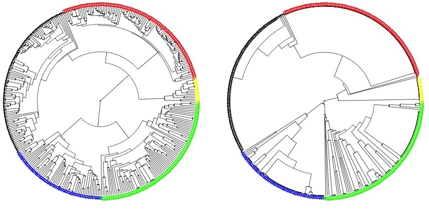
Figure 1: Circular dendrogram generated by the same technique as in Zhao et al. (2011)(left) and $WR$ (right), for the RICE data. Green, blue, red, yellow, and black indicate indica, aus, temperate japonica, aromatic and tropical japonica, respectively.

4.2.3 Gene expression data

In this example we demonstrate that the performance of $WR$ can be regarded as robust. Consider the gene expression data presented and analyzed in Alizadeh et al. (2000). It is actually classification data and analyzed as such in Dudoit et al. (2002). Here, for demonstration purposes we compare some of the clusterings we can generate to the known classes so as to find CRs. The sample size is 62 and there are three classes: diffuse large B-cell lymphomas (D) with 42 samples, follicular lymphoma (F) with 9 samples, and chronic lymphocytic leukemia (C) with 11 samples. The dimension of the gene expression data after pre-processing is 4026. (The pre-processing included normalization, imputation, log transformation, and standardization to zero mean and unit variance across genes.)

First we applied $K$-means to the data 1000 times with $K=3$ and random starts, and found an average CR of 0.79 with a standard error of 0.13. When we applied $MWKM$ to the data, we found its CR to be 0.67, noticeably worse than $K$-means.

Now consider the following procedure. Trichotomize all 4026 variables by using their 33% and 66% percentiles and relabel them as ‘1’, ‘2’, and ‘3’. Then, apply $WOR$ and $WR$ to the discretized data. To get CRs for hierarchical methods, we must convert their dendrograms to clusterings by cutting them at some level. To do this, we used the function cuttree (with $K=3$) in R. The resulting CRs for $WOR$, $WR$ were 0.71 and 0.84, respectively. That is, even when the data are discrete only because they were made that way artificially, $WR$ handily outperformed three other methods.

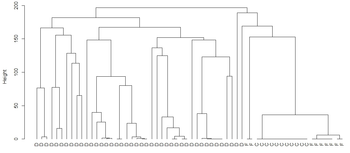
Figure 2: Dendrogram of WR.

The full dendrogram from $WR$ is given in Fig. 2. Along the horizontal axis, the correct labels of the classes are given. If these were ignored and one were merely to eyeball the data, one could be led to put the two rightmost D’s and the first two F’s into the cluster of C’s, giving an CR of 58/62 = .93 – much higher than .84. One could just as well put the leftmost D’s into one cluster, the next 13 D’s into a second cluster, the next eight D’s into a third cluster, and the rightmost 18 observations into a fourth cluster, leaving the intervening data points essentially as a fifth cluster that does not cohere. In this case, the CR would be terrible. So, even though the data are artificially discretized, using an automated method of $WR$ on a discretized $WR$ and cutree gives a result in the midrange of what informal methods would give. This is evidence that ensemble methods such as $WR$ are inherently robust. Otherwise put, reading dendrograms informally can be misleading whereas formal methods may be reliably accurate.

5 Extension to high dimensional vectors of unequal length

We extend our method to clustering categorical vectors of different lengths. This is an important clustering problem in genomics because it is desirable to be able to cluster strains of organisms, for instance, even though their genomes have different lengths in terms of number of nucleotides. The first step is to preprocess the data so all the vectors have the same length. This process is called alignment. The aligned vectors can then be clustered using the technique of Sec. 4. The point of this section is to verify that our clustering method is effective even after alignment.

To be specific, consider sequence data of the form ${\cal{X}}_{i}=(x_{i1}x_{i2}...x_{iJ_{i}})$ with $i=1,\ldots,n$ in which each $x_{ij}$ for $j=1,\ldots,J_{i}$ is a nucleotide in $\{A,T,C,G\}$. It is obvious that a sufficient condition for our method to apply is that all the $x_{ij}$’s assume values in sets $A_{j}$ for which $\#(A_{j})$ is bounded. To find a common value for the $n$ sequences we align them using software called MAFFT-7 (Katoh and Standley (2013)). MAFFT-7 is a multiple alignment program for amino acid or nucleotide sequences. The basic procedure was first presented in Needleman and Wunsch (1970). A recent comparison of algorithms and software for this kind of alignment problem was carried out in Katoh and Standley (2013) who argued that MAFFT-7 is faster and scales up better than other implementations such as CLUSTAL and MUSCLE.

At the risk of excessive oversimplification, the basic idea behind alignment procedures is as follows. Suppose two sequences $x_{i}$ and $x_{k}$ of different lengths are to be aligned. Then, the alignment procedure introduces place holders represented by $\phi$ so that the two sequences are of the same length and the subsequences that do match are in the same place along the overall sequence. When more than two sequences must be aligned, a progressive alignment can be used, i.e., two sequence are aligned and fixed, the third one aligned to previous ones, and the procedure continues until all sequences are aligned. Given that a collection of genomic sequences have been aligned, we can cluster them by applying our technique.

In the absence of established theory for this more complicated case, we present two examples to verify that the procedure gives reasonable results. Both of our examples concern viruses: Their genomes are large enough to constitute a nontrivial test of our clustering method and of different enough in lengths from species to species that alignment of some sort is necessary.

As a first simple example, consider the virus family Filovirdae . This family includes numerous related viruses that form filamentous infectious viral particles (virions). Their genomes are represented as single-stranded negative-sense RNAs. The two members of the family that are best known are Ebolavirus and Marburgvirus. Both viruses, and some of their lesser known relatives, cause severe disease in humans and nonhuman primates in the form of viral hemorrhagic fevers (see Pickett et al. (2012)).
There are three genera in Filoviridae, and we chose as our data set all the complete and distinct viral genomes with a known host from this family available from ViPR. There were 103 in total from 3 genera, namely, Cuevavirus (1, Cue), Ebolavirus (80), and Marburgvirus (22, Mar) where the indicators in parentheses show the frequency and the abbreviation. Ebolavirus further subdivides into five species: Bundibugyo virus (3, Bun), Reston ebolavirus (5, Res), Sudan ebolavirus (6, Sud), Tai Forest ebolavirus (2, Tai), and Zaire ebolavirus (64, Zai). The hosts are human, monkey, swine, guinea pig, mouse, and bat (denoted hum, mon, swi, gpi, mou, bat, respectively, on the dendrograms). The minimum and maximum genome lengths are 18623 and 19114. While we recognize that the genomes in the pathogen virus resource are not drawn independently from a population, we can nevertheless apply our method and evaluate the results.

We apply only $WR$ as $WOR$ and $MWKM$ performed poorly on high dimensional data. In addition, we used $HCSL$, $HCCL$, and $HCAL$ because we had a dissimilarity that could be used after alignment. Essentially, as long as the distance between $\phi$ and the nucleotides could be omitted from the Hamming distance sum, the dissimilarity was well-defined. It turned out that all three gave nearly identical results although $HCAL$ was slightly better. The important point is that $WR$ performed better than the three non-ensemble methods because the ensembling over dissimilarity matrices gives a better assessment of the distance between aligned genomes than not ensembling.

The results for $HCAL$ are shown in the Fig. 4. It is seen that the subpopulations are well separated. Virologically speaking, this means that the various species correspond to relatively tight clusters. Within the Marburg cluster (on the left) it appears that most of the genomes have either humans or bats as hosts suggesting that one organism (probably the bats) is transmitting Marburg to the other (probably human). Sudan ebolavirus mainly afflicts humans (pending more data) while Reston ebolavirus is known not to be a pathogen for humans. The vast majority of the Zaire and Bunibugyo genomes have human as host.

Fig. 4 shows the corresponding dendrogram using $WR$, an ensemble method. Qualitatively the results are the same as for $HCAL$. The improvement of $WR$ over $HCAL$ is seen in the fact that $WR$ reveals greater separation between the clusters. Indeed, even if one corrects for the vertical scale, the leaves within a cluster under $WR$ separate from each other at a much finer level. That is, the ensembling over the dissimilarities accentuates the differences between genomes in different clusters as discussed in Sec. 3.2.

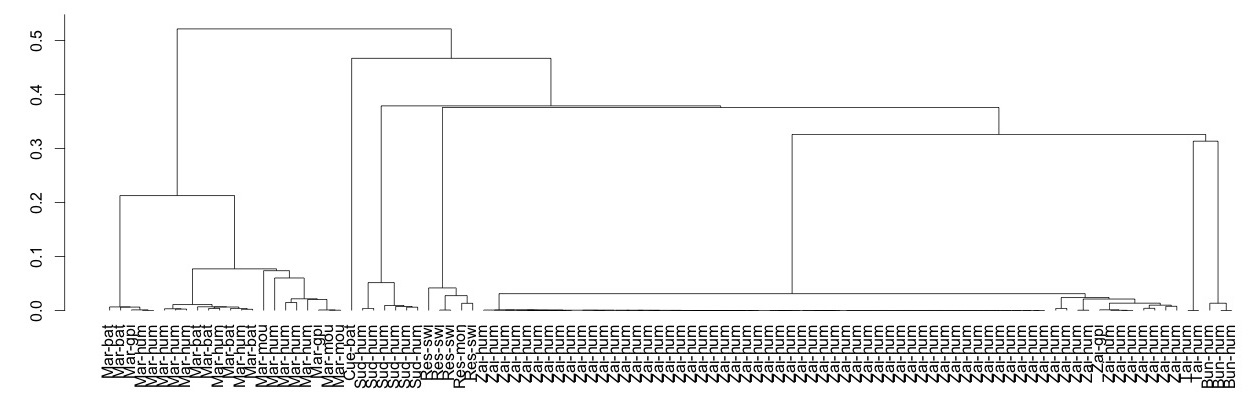
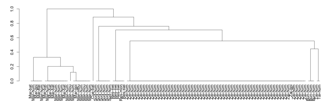
Figure 3: Dendrogram for the Filoviridae data set using $HCAL$. The leaves are labeled with the Genus or species and host.

Figure 4: Dendrogram for the Filoviridae data set using $WR$ under the same labeling convention as the Fig. 4.

These dendrograms can be contrasted with a phylogenetic tree for the Filoviridae viruses. Figure 5 shows the phylogenetic tree generated by the neighbor-joining (NJ) method as implemented in the R package Ape (Paradis et al. (2004)). The NJ method constructs a tree by successive pairing of the neighbors. The idea behind a phylogenetic tree, as opposed to a dendrogram, is to represent the sequence of evolutionary steps through which organisms mutated as a reasonable way to classify the existing and extinct organisms. The goals of the two sorts of trees are somewhat different and one would not expect them to agree fully, since clustering only gives a mathematically optimal path to the evolutionary endpoint while phylogenetic trees try to track genomic changes. For instance, the phylogenetic tree shows that Zaire ebolavirus with a human host separates early into two distinct groups which may or may not be reasonable evolutionarily and is different from Fig. 4. Tai Forest ebolavirus and Bunidbugyo virus genomes are seen to be possibly close evolutionary but are not close in Fig. 4. On the other hand, Sudan ebolavirus and Reston ebolavirus are seen to be close in terms of both clustering and phylogenetics while Marburg is a separate and recent genus, consistent with it being its own cluster.

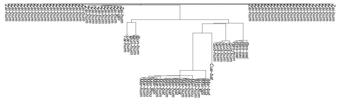
Figure 5: Phylogenetic tree generated for Filoveridae by NJ. It is broadly similar to the dendrograms in Figs. 4 and 4, but differs in some details.

As a second and more complicated example, we studied the Herpesviridae family of viruses that cause diseases in humans and animals. Herpesviridae is a much larger family than Filoviridae and the genomes in Herpesviridae are generally longer as well as more varied in length than those in Filoviridae. According to ViPR, the family Herpesviridae is divided into three subfamilies (Alphaherpesvirinae, Betaherpesvirinae and Gammaherpesvirinae). We limited our analysis to the distinct and complete genomes in Alphaherpesvirinae that have known hosts; Alphaherpesvirinae has more complete genomes than either Betaherpesviridae or Gammaherpesvidae. Within Alphaherpesviridae there are has five genera: Iltovirus (IIt), Mardivirus (Mar), Scutavirus, Simplexvirus (Sim), and Varicellovirus (Var). Since Scutavirus did not have complete any complete genomes, we disregarded this genus. The rest remaining genera had 20, 18, 20, 40 genomes, respectively, from different hosts, namely, human, Monkey, chicken, Turkey, Duck, cow, Bat (Fruit), equidae (horse), Boar, Cat family, Amazona oratrix (denoted hum, mon, chi, tur, duc, cow, bat, equ, boa, cat, and ora, respectively in the dendrograms). These viral genomes have lengths ranging from 124784 to 178311 base pairs.

Parallel to the Ebolavirus example, we present the two dendrograms corresponding to $HCAL$ and $WR$. These are in Fig.8 and 8. The top panel shows that $HCAL$, the non-ensembled version based on Hamming distance, is qualitatively the same as the lower panel. As before, the key difference is that $WR$ yields a cleaner separation of clusters relative to $HCAL$. It is important to note that the clusters in the dendrograms correspond to (genus, host) pairs. That is, the clustering corresponds to identifiable physical differences so the clusters have a clear interpretation.

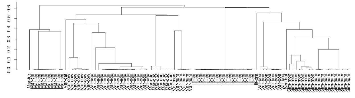
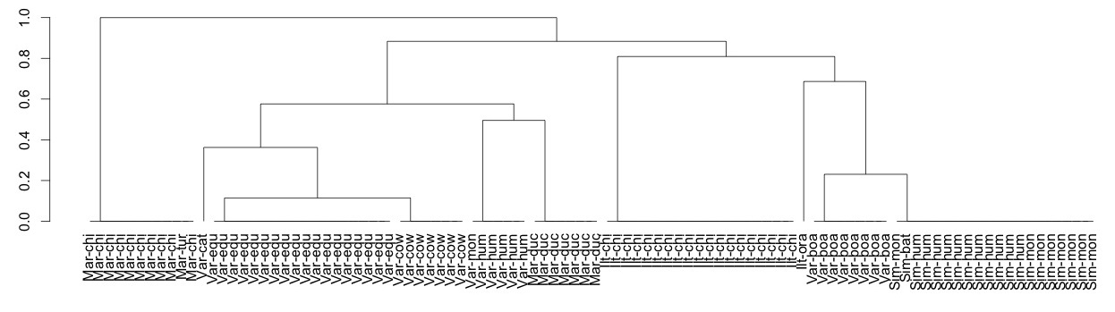
Figure 6: Dendrogram for the Alphaherpesviridae data set using $HCAL$. The leaves are labeled with the genome Genus or subpopulation and host.

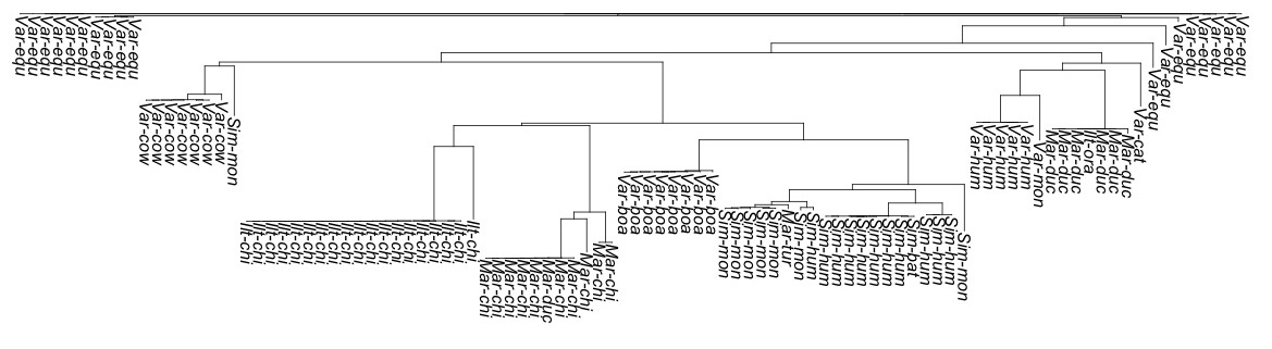
Figure 7: Dendrogram for the Alphaherpesviridae data set using $WR$ under the same labeling convention as the top panel.

Figure 8: Phylogenetic tree generated for Alphaherpesviridae. It is broadly similar to the dendrograms in Figs. 8 and 8, but differs in some details.

The same cannot be said for the phylogenetic tree generated by NJ as before and shown in Fig. 8. For instance, Varicellovirus from host equidae are partitioned into two clusters early. Also, Mardivirus from chicken and duck hosts are not cleanly separated. On the other hand, most other population-host pairs are fairly well separated. Overall, Fig. 8 does not give as good a clustering as the panels in Figs. 8 and 8.

6 Conclusions

In this paper we have presented a method for clustering categorical data in low, high, and varying dimensions. We began with relatively small dimensions, up to 35 for the ${\sf SOYBEAN}$ data, and studied the way our method seemed to improve over other methods. Specifically, we ensembled over dissimilarity matrices in an effort to represent the distance between data points more accurately. Our theoretical work in Sec. 3.2 provides some formal justification for why this sort of technique should perform well in some generality.

Then we turned to the clustering of high dimensional categorical data, focusing on genomic data. We extended our ensemble method for low dimensional data to high dimensional categorical vectors of equal length by adding a layer of ensembling: We obtained dissimilarity matrices by ensembling over randomly selected dimensions. We then used our method on categorical vectors of different lengths by artificially making them the same length through alignment procedures. Again, our ensembling method performed better than the other methods we tested. In particular, we compared the output of our method in this case to phylogenetic trees. While not strictly scientific, the dendrograms we generated can be interpreted physically and differ in some important respects from phylogenetic trees generated from the same data.

Throughout we have used a large number of simulated and real data examples to buttress the intuition behind the technique and formal results. We comment that there are many other tests of the general methodology that could be done. For instance, in our clustering of viral genomes we could have included incomplete genomes. However, it many cases the incomplete genomes had over 90% of the nucleotides missing and we thought this insufficient for good conclusions.

References

- Alizadeh et al. (2000) Alizadeh, A. A., M.B. Eisen, R.E. Davis, C. Ma, I.S. Lossos, et al. (2000), ”Distinct types of diffuse large B-cell lymphoma identified by gene expression profiling,” Nature, 403(6769), 503-511.
- Amiri et al. (2015) Amiri, S., B. Clarke, J. Clarke, and H. Koepke (2015), ”A general hybrid clustering technique,” arXiv preprint arXiv:1503.01183.
- Andreopoulos and Wang (2007) Andreopoulos, B., A. An, and X. Wang (2007), ”Hierarchical density-based clustering of categorical data and a simplification,” In Advances in Knowledge Discovery and Data Mining (11-22). Springer Berlin Heidelberg.
- Bai et al. (2012) Bai, L., J. Liang, C. Dang, and F. Cao (2012), ”A cluster centers initialization method for clustering categorical data,” Expert Systems with Applications, 39(9), 8022-8029.
- Bai et al. (2011) Bai, L., Liang, J., Dang, C., and F. Cao (2011), ”A novel attribute weighting algorithm for clustering high-dimensional categorical data,” Pattern Recognition, 44(12), 2843-2861.
- Bellman et al. (1961) Bellman, R.E. (1961), ”Adaptive control processes: a guided tour”. Princeton University Press.
- Beyer et al. (1999) Beyer, K., J. Goldstein, R. Ramakrishnan, and U. Shaft (1999), ”When is nearest neighbor meaningful?,” In Database Theory-ICDT’99 (pp. 217-235). Springer Berlin Heidelberg.
- Breiman (1996) Breiman, L (1996), ”Bagging predictors,” Machine learning, 24(2), 123-140.
- Cao et al. (2009) Cao, F., Liang, J., and L. Bai (2009), ”A new initialization method for categorical data clustering,” Expert Systems with Applications, 36(7), 10223-10228.
- Celeux and Govaert (1991) Celeux, G. and G. Govaert (1991), ”Clustering Criteria for Discrete Data and Latent Class Models,” Journal of Classification, 8, 157-176.
- Chan et al. (2004) Chan, E. Y., W.K. Ching, M.K. Ng, and J.Z. Huang (2004), ”An optimization algorithm for clustering using weighted dissimilarity measures,” Pattern recognition, 37(5), 943-952.
- Chang (1983) Chang, W.C (1983), ”On using principal components before separating a mixture of two multivariate normal distributions,” Applied Statistics, 267-275.
- Dudoit et al. (2002) Dudoit, S., J. Fridlyand, and T. P. Speed (2002), ”Comparison of discrimination methods for the classification of tumors using gene expression data,” Journal of the American statistical association, 97(457), 77-87.
- Ester et al. (1996) Ester, M., H.P. Kriegel., J. Sander, and X. Xu (1996), ”A density- based algorithm for discovering clusters in large spatial databases with noise,” In: Proc. 2nd Internat. Conf. Knowl- edge Discovery and Data Mining (KDD-96), Portland, OR, pp. 226-231.
- Fraley and Raftery (2002) Fraley, C., and A.E. Raftery (2002), ”Model-based clustering, discriminant analysis, and density estimation,” Journal of the American Statistical Association, 97(458), 611-631.
- Fred and Jain (2005) Fred, A.L. and A.K. Jain (2005), ”Combining multiple clusterings using evidence accumulation”. Pattern Analysis and Machine Intelligence, IEEE Transactions on, 27(6), 835-850.
- Friedman and Meulman (2004) Friedman, J.H., and J.J. Meulman (2004), ”Clustering objects on subsets of attributes (with discussion),” Journal of the Royal Statistical Society: Series B (Statistical Methodology), 66(4), 815-849.
- Ganti et al. (1999) Ganti, V., J. Gehrke, and R. Ramakrishnan (1999), ”CACTUS-clustering categorical data using summaries,” In Proceedings of the fifth ACM SIGKDD international conference on Knowledge discovery and data mining, (73-83), ACM.
- Guha et al. (1999) Guha, S., R. Rastogi, and K. Shim (1999), ”ROCK: A robust clustering algorithm for categorical attributes,” In Data Engineering,. Proceedings., 15th International Conference on, (512-521), IEEE.
- Hall et al. (2005) Hall, P., J.S. Marron, and A. Neeman (2005), ”Geometric representation of high dimension, low sample size data,” Journal of the Royal Statistical Society: Series B (Statistical Methodology), 67(3), 427-444.
- He et al. (2005) He, Z., X. Xu, and S. Deng (2005), ”A cluster ensemble method for clustering categorical data,” Information Fusion, 6(2), 143-151.
- Huang (1998) Huang, Z (1998), ”Extensions to the v-means Algorithm for Clustering Large Data Sets with Categorical Values,” Data Mining and Knowledge Discovery, 2, 283-304.
- Iam-On et al. (2012) Iam-On, N., T. Boongeon, S. Garrett and C. Price (2012), ”A link-based cluster ensemble approach for categorical data clustering,” Knowledge and Data Engineering, IEEE Transactions, 24(3), 413-425.
- Jing et al. (2007) Jing, L., M.K. Ng, and J.Z. Huang (2007), ”An entropy weighting k-means algorithm for subspace clustering of high-dimensional sparse data,” Knowledge and Data Engineering, IEEE Transactions on, 19(8), 1026-1041.
- Katoh and Standley (2013) Katoh, K., and D.M. Standley (2013), ”MAFFT multiple sequence alignment software version 7: improvements in performance and usability,” Molecular biology and evolution, 30(4), 772-780. http://mafft.cbrc.jp/alignment/software/
- Khan and Ahmad (2013) Khan, S. S., and A. Ahmad (2013), ”Cluster Center Initialization Algorithm for -modes Clustering,” Expert Systems With Applications,40(18), 7444-7456.
- Kriegel et al. (2009) Kriegel, H.P., P. Kröger, and A. Zimek (2009), ”Clustering high-dimensional data: A survey on subspace clustering, pattern-based clustering, and correlation clustering,” ACM Transactions on Knowledge Discovery from Data (TKDD), 3(1), 1.
- Kuhn (2005) Kuhn, H. W (2005), ”The Hungarian method for the assignment problem,” Naval Research Logistics (NRL), 52(1), 7-21.
- Larkin (2007) Larkin, M. A., G. Blackshields, N.P. Brown, et al. (2007), ”Clustal W and Clustal X version 2.0,” Bioinformatics, 23(21), 2947-2948.
- Lichman (2013) Lichman, M.(2013), ”UCI Machine Learning Repository,” http://archive.ics.uci.edu/ml, University of California, Irvine, School of Information and Computer Sciences.
- Murtagh (2004) Murtagh, F. (2004), ”On ultrametricity, data coding, and computation,” Journal of Classification, 21, 167-184.
- Needleman and Wunsch (1970) Needleman, S.B. and C.D. Wunsch (1970), ”A general method applicable to the search for similarities in the amino acid sequences of two proteins,” J. Mol. Biol., 48:443-453.
- Paradis et al. (2004) Paradis E., J. Claude, and K. Strimmer (2004), ”APE: analyses of phylogenetics and evolution in R language,” Bioinformatics 20: 289-290. doi:10.1093/bioinformatics/btg412.
- Parsons et al. (2004) Parsons, L., E. Haque, and H. Liu (2004), ”Subspace clustering for high dimensional data: a review,” ACM SIGKDD Explorations Newsletter, 6(1), 90-105.
- Pickett et al. (2012) Pickett, B. E., E. L. Sadat, Y. Zhang, Noronha, et al. (2012), ”ViPR: an open bioinformatics database and analysis resource for virology research,” Nucleic acids research, 40(D1), D593-D598. www.viprbrc.org
- Purcell et al. (2007) Purcell, S., B. Neale, K. Todd-Brown, L. Thomas, M. Ferreira, D. Bender, J. Maller, P. Sklar, P. de Bakker, M. Daly, and P.C. Sham (2007), ”PLINK: a toolset for whole-genome association and population-based linkage analysis,” American Journal of Human Genetics, 81. http://pngu.mgh.harvard.edu/purcell/plink/
- Strehl and Ghosh (2002) Strehl, A., J. Ghosh (2002), ”Cluster ensembles–a knowledge reuse framework for combining multiple partitions,” Journal on Machine Learning Research, 3, 583-617.
- Steinbach et al. (2004) Steinbach, M., L. Ertöz, and V. Kumar (2004), ”The challenges of clustering high dimensional data,” In New Directions in Statistical Physics, (pp. 273-309), Springer Berlin Heidelberg.
- Witten and Tibshirani (2010) Witten, D. M., and R. Tibshirani (2010), ”A framework for feature selection in clustering,” Journal of the American Statistical Association, 105(490), 713-726.
- Wu at al. (2007) Wu, S., Q. Jiang, and J.Z. Huang(2007), ”A new initialization method for clustering categorical data,” In: Advances in Knowledge Discovery and Data Mining, 972-980. Springer, Berlin.
- Yeung and Ruzzo (2001) Yeung, K.Y., and W.L. Ruzzo (2001), ”Principal component analysis for clustering gene expression data,” Bioinformatics, 17(9), 763-774.
- Zaki et al. (2007) Zaki, M. J., M. Peters, I. Assent, and T. Seidl (2007), ”Clicks: An effective algorithm for mining subspace clusters in categorical datasets,” Data & Knowledge Engineering, 60(1), 51-70.
- Zhang et al. (2006) Zhang, P., X. Wang, and P.X.K. Song (2006), ”Clustering categorical data based on distance vectors,” Journal of the American Statistical Association, 101(473), 355-367.
- Zhao et al. (2011) Zhao, K., C.W. Tung, G.C. Eizenga, M.H. Wright, Ali, et al. (2011),” Genome-wide association mapping reveals a rich genetic architecture of complex traits in Oryza sativa,” Nature communications, 2, 467.