Core-Collapse Supernova Rate Synthesis Within 11 Mpc

Abstract

The 11 Mpc ${\rm H\alpha}$ and Ultraviolet Galaxy (11HUGS) Survey traces the star formation activity of nearby galaxies. In addition within this volume the detection completeness of core-collapse supernovae (CCSNe) is high therefore by comparing these observed stellar births and deaths we can make a sensitive test of our understanding of how stars live and die. In this paper, we use the results of the Binary Population and Spectral Synthesis (BPASS) code to simulate the 11HUGS galaxies’ ${\rm H\alpha}$ and far-ultraviolet (FUV) star formation rate indicators (SFRIs) and simultaneously match the core-collapse supernova (CCSN) rate. We find that stellar population including interacting binary stars makes little difference to the total CCSN rate but increases the ${\rm H\alpha}$ and FUV fluxes for a constant number of stars being formed. In addition they significantly increase the predicted rate of type Ibc supernovae (SNe) relative to type II SNe to the level observed in the 11HUGS galaxies. We also find that instead of assuming a constant star formation history (SFH) for the galaxies our best fitting models have a star formation rate (SFR) that peaked more than 3 Myrs ago.

1 Introduction

Core-collapse supernovae (CCSNe) are the explosive events that mark the death of massive stars ($\ga 8{\rm M_{\odot}}$) (Smartt et al., 2009). They are classified into hydrogen-rich events, Type IIP/L/n/b, and hydrogen-deficient events, type Ib/c, according to the presence or absence of hydrogen lines in their spectrum (Filippenko, 1997). This is directly related to the composition of the outer layers of a progenitor star at the moment of explosion. Type II supernova (SN) progenitors have kept their hydrogen rich outer envelope intact, while type Ib/c have lost the hydrogen envelope. The most direct evidence linking the star that explodes to the type of SN is from direct detection of the progenitor in pre-explosion images (e.g. Li et al., 2007; Smartt, 2009). Non-detections of progenitors in pre-explosion images for type Ibc SN were used by Eldridge et al. (2013) to indicate the important effect of interacting binary stars on determining the CCSN progenitor diversities and local CCSN rate. This idea was later reinforced by the probable detection of a binary system progenitor for the type Ibc SN iPTF13bvn (Cao et al., 2013; Bersten et al., 2014; Eldridge et al., 2015).

However, it is difficult to directly detect CCSN progenitors because the event must occur in a galaxy within about 30 Mpc that has been imaged by the Hubble Space Telescope before explosion. Therefore indirect methods must be exploited to gain further insight into CCSNe. The most useful methods include the relative rates of different CCSN types (e.g. Podsiadlowski et al., 1992; De Donder & Vanbeveren, 1998; Hakobyan, 2008; Eldridge et al., 2008; Boissier & Prantzos, 2009; Smith et al., 2011), the stellar populations surrounding the site of CCSNe (e.g. Williams et al., 2014) and the location of CCSNe within their host galaxies (e.g. Fruchter et al., 2006; James & Anderson, 2006; Kelly et al., 2008; Anderson et al., 2012).

One other interesting constraint on CCSNe and their progenitors can be obtained by exploiting the link between stellar deaths and stellar births. This was attempted by Botticella et al. (2012). They used the 11HUGS galaxy catalogue that lists the ${\rm H\alpha}$ and FUV fluxes for a large number of galaxies within 11 Mpc. These fluxes are commonly used tracers of recent star formation (Kennicutt, 1998). The amount of ${\rm H\alpha}$ and FUV emitted are determined by the most massive hot stars that evolve quickly and explode as CCSNe a few million years after their formation. Botticella et al. (2012) were able to show that the observed ${\rm H\alpha}$ and FUV fluxes from the 11HUGS galaxies were consistent with the observed CCSN rate for the galaxies if the minimum stellar mass for a CCSN to occur was $8{\rm M_{\odot}}$, in agreement with results from CCSN progenitor detection in Smartt et al. (2009).

This study was repeated by Horiuchi et al. (2013) who tried a slightly more sophisticated modelling of the 11HUGS galaxies. Rather than using the canonical expected SFR conversion factors from Kennicutt (1998) they estimated the expected ${\rm H\alpha}$, FUV flux and CCSN rate from the latest stellar models including rotation calculated by Ekström et al. (2012). Over the last few decades the understanding of how rotation affects stellar evolution has significantly advanced (see reviews by Maeder & Meynet, 2000; Langer, 2012). The general effect is to increase the main-sequence life time and temperature of massive stars as they evolve so lead to more ${\rm H\alpha}$ and FUV flux being emitted for the same SFR. Horiuchi et al. (2013) found that it is possible that there could be a CCSN rate excess as well as that the observations disfavoured the rotating models as they made this SN rate excess worse.

There is a second important factor left for our stellar population models that is the effect of interacting binaries. When two stars are orbiting each other in a binary-star system the opportunity for mass transfer between the two stars arises. The more massive star typically evolves faster than the less massive star, fills its Roche-Lobe and transfers mass to the companion star. This produces more hot and luminous stars and therefore has similar observed consequence as stellar rotation does (e.g. Vanbeveren et al., 1998; Eldridge et al., 2008; Zhang & Li, 2012). However the situation may be more complex as there is evidence that the most rapid rotation only occurs in binary systems (de Mink et al., 2013).

In this paper we continue the work of Botticella et al. (2012) and Horiuchi et al. (2013) by attempting to match the observed ${\rm H\alpha}$, FUV fluxes and CCSN rate in the 11HUGS galaxies. We will use the Binary Population and Spectral Synthesis (BPASS, http://bpass.auckland.ac.nz) code that accounts for the impact of interacting binaries on stellar populations (Eldridge & Stanway 2009, 2012). The BPASS code has been tested against a number of different observables that are dependant on the evolution of massive stars. Our aim is to apply a simple test to BPASS models to reproducing the CCSN rate, ${\rm H\alpha}$ and FUV fluxes. Our work concentrates on the effect of interacting binary stars on the CCSN rate of their host galaxies. We also include two other refinements to our models. First we reproduce the chemical compositions of the 11HUGS galaxies based on the B-band magnitude of nearby galaxies sample rather than using a Solar composition population. Second we allow the SFH to vary rather than assuming only a constant SFR.

The structure of this paper is arranged as follows. In Section 2, we introduce the 11HUGS and CCSN samples and how we determine the metallicity of the 11HUGS galaxies. In the following Section 3, we summarise the effect of interacting binary stars on CCSN rate and SFRIs we find from the BPASS code’s results. We also outline how we use these BPASS results to construct our synthetic galaxy models. In Section 4, we compare our models to observations before finally discussing our results and presenting our conclusions in Section 5.

2 Galaxy and CCSNe samples

Table 1: Nearby galaxy sample from the 11 HUGS survey (Lee et al., 2004; Botticella et al., 2012) and CCSNe sample from Eldridge et al. (2013): Numbers of galaxies, the total ${\rm L_{H\alpha}/10^{43}erg\,s^{-1}}$, ${\rm L_{UV}/10^{28}erg\,s^{-1}Hz^{-1}}$ and CCSN rate (${\rm R_{CC}/yr^{-1}}$). ¹The ${\rm L_{UV}}$ for Sample A is an estimation with respect to the relative ratio of ${\rm H\alpha}$ and UV flux from Sample B and C.

Parameter	Sample A	Sample B	Sample C
${\rm N_{gal}}$	383	312	167
${\rm L_{H\alpha}/10^{43}erg\,s^{-1}}$	${\rm 1.1\pm 0.05}$	${\rm 0.9\pm 0.05}$	${\rm 0.7\pm 0.04}$
${\rm L_{UV}/10^{28}erg\,s^{-1}Hz^{-1}}$	${}^{1}{106\pm 8}$	${\rm 88\pm 6}$	${\rm 67\pm 4}$
${\rm N_{CC}}$	17	15	14
${\rm N_{SNI}}$	4	4	3
${\rm N_{SNII}}$	13	11	11
${\rm R_{CC}/yr^{-1}}$	${\rm 1.13\pm 0.27}$	${\rm 1\pm 0.26}$	${\rm 0.93\pm 0.25}$

The galaxy samples we adopt in this paper are drawn from Botticella et al. (2012). There are three different samples: 383 galaxies with measured flux in ${\rm H\alpha}$ (sample A), 312 galaxies with measured fluxes in ${\rm H\alpha}$ and FUV (sample B) and 167 galaxies with measured fluxes in ${\rm H\alpha}$, FUV and Total Infrared (TIR) (sample C). We list the observed fluxes of these samples in Table 1. We broadly assume that the relative ratio of ${\rm H\alpha}$ and FUV flux is constant. Therefore applying the averaged flux ratio of ${\rm H\alpha}$ and FUV of Sample B and C to Sample A, we estimate the FUV luminosity of Sample A: ${\rm L_{UV}=(106\pm 8)\times 10^{28}erg\,s^{-1}Hz^{-1}}$.

In addition, we list the details of the 17 CCSNe discovered within 11 Mpc from 1998 to 2012 in Table 2. It is directly based on the work of Botticella et al. (2012), where they picked out all identified SNe occurred in galaxy sample A of 11HUGS survey from 1885 to 2010 from the Asiago SNe catalogue (Barbon et al., 2008). We limit our SNe sample to only core-collapse events. We also extend this CCSN list up to 2012 using the SN list from Eldridge et al. (2013). This list of SNe was compiled by searching the catalogue maintained by the International Astronomical Union (IAU) Central Bureau for Astronomical Telegrams (CBET). It was searched for all SNe discovered in the fifteen-year period from 1 Jan 1998 to 30 March 2012. The host galaxies of these selected SNe have a recessional velocity (corrected for Local Group infall on Virgo) of 2000 $\rm{kms^{-1}}$ or less, corresponding to a distance limit of 28 Mpc for $\rm{H_{0}=72kms^{-1}Mpc^{-1}}$.

All CCSNe used in our work is in the field of 11HUGS survey and related to the adopted SFRIs. Of these there are 13 type II SNe and 4 type Ibc SNe. Among all the CCSNe host galaxies, the host galaxy of SN 2005at is in Sample A and B but not in Sample C, and the host galaxy of both SN 2005af and SN 2011ja is only in Sample A. It is important to consider whether our sample of SN is complete and whether there might have been some CCSNe unobserved. For example some CCSNe might occur in very dusty regions of galaxies and remain unobserved or some SNe might form black holes and remain unobserved (e.g. Smartt, 2015). However modern SN searches are unlikely to have missed many SNe. In addition if any SNe are unobservable due to dust, their associated ${\rm H\alpha}$ and FUV emission will also be decrease thus in this work should not contribute to the observed SFRIs. Although in light of these concerns we can suggest that our CCSN rate is at least a robust lower limit.

Table 2: CCSNe discovered within 11 Mpc from 1998 to 2012 as listed by Eldridge et al. (2013). ¹SN 2005at host galaxy NGC 6744 is in Sample A and B not in Sample C ,²SN 2005af and SN 2011ja host galaxy NGC 4945 is only in Sample A.

SN	Gal.	Type	${\rm M_{B}}$	D/Mpc
2002ap	NGC 628	Ic	-19.65	7.3
2002bu	NGC 4242	IIn	-18	7.4
2002hh	NGC 6946	IIP	-20.65	5.9
2003gd	NGC 628	IIP	-19.65	7.3
2004am	NGC 3034	IIP	-19.08	3.53
2004dj	NGC 2403	IIP	-18.77	3.22
2004et	NGC 6946	IIP	-20.65	5.9
2005cs	NGC 5194	IIP	-20.7	8
2007gr	NGC 1058	Ic	-18.2	9.2
2008ax	NGC 4490	IIb	-19.39	8
2008bk	NGC 7793	IIP	-18.41	3.91
2009hd	NGC 3627	IIP	-19.61	10.05
2011dh	NGC 5194	IIb	-20.7	8
2012fh	NGC 3344	Ic	-18.8	6.6
1 2005at	NGC 6744	Ic	-20.9	9.4
2 2005af	NGC 4945	IIP	-20.6	4.08
2 2011ja	NGC 4945	IIP	-20.6	4.08

3 Method

Our method to reproduce the 11HUGS ${\rm H\alpha}$ flux, UV flux and CCSN rate falls into three steps. First a metallicity classification of the 11HUGS galaxies is applied so that we can blend our models of different metallicities and obtain a more realistic simulation of 11HUGS sample. Second we describe the BPASS stellar population model that we use to construct our models, and discuss the effect of interacting binary stars on CCSN rate and SFRIs of star-forming galaxies. Finally we outline our method to create a synthetic galaxy model with various star-formation histories.

3.1 Metallicity Classification

Table 3: Metallicity classification of Sample B galaxies: the fraction of total galaxies, ${\rm H\alpha}$ flux, FUV flux and number of CCSNe when the 11HUGS galaxies are divided into the 5 metallicities of BPASS.

	Z	${\rm[O/H]}$	${\rm f_{gal}}$	${\rm f_{H\alpha}}$	${\rm f_{FUV}}$	${\rm f_{CCSN}}$
${\rm T04}$	0.001	$7.5$	0.178	0.003	0.002	0
	0.004	$8.1$	0.451	0.038	0.033	0
	0.008	$8.4$	0.197	0.134	0.096	0.057
	0.020	$8.8$	0.117	0.324	0.253	0.531
	0.040	$9.0$	0.057	0.501	0.616	0.412
${\rm KK04}$	0.001	$7.5$	0.083	0.001	0.001	0
	0.004	$8.1$	0.292	0.009	0.009	0
	0.008	$8.4$	0.317	0.052	0.04	0
	0.020	$8.8$	0.225	0.339	0.258	0.353
	0.040	$9.0$	0.083	0.599	0.692	0.647
${\rm PP04}$	0.001	$7.5$	0	0	0	0
	0.004	$8.1$	0.498	0.052	0.043	0
	0.008	$8.4$	0.419	0.427	0.324	0.294
${\rm O3N2}$	0.020	$8.8$	0.079	0.521	0.633	0.706
	0.040	$9.0$	0.003	0	0	0

Previous studies have only considered reproducing the stellar populations in 11HUGS samples by using only Solar metallicity composition for the stellar populations. However it is well known that synthetic population results depend on metallicity even when interacting binaries are included. Therefore we take account of the varying chemical compositions of the 11HUGS galaxies. We estimate the galaxies’ metallicity by using the luminosity-metallicity (L-Z) relation of the SDSS galaxies provided by Tremonti et al. (2004). This shows generally good agreement with other local samples of galaxies. The relation is,

$$[O/H] = 12+\log(O/H)$$ (1)

$$= -(0.185\pm 0.001)M_{B}+(5.238\pm 0.018)$$

The ratio of oxygen and hydrogen [O/H], is a common measurement of galaxy metallicity and able to be estimated by the B-band magnitude of the host galaxy taken from Lee et al. (2011). However, this L-Z relation is strongly affected by dust attenuation and the choice of which strong-line abundance calibrations are used as discussed in Kewley & Ellison (2008). To quantify the influence of dust, Tremonti et al. (2004) correct the galaxy luminosities for intrinsic attenuation using the attenuation curve of Charlot & Fall (2000) and assume that the stars experience one third of the attenuation measured in nebular gas. To account for the effect of using different strong-line abundance calibrations, we use the work of Kewley & Ellison (2008) who derived conversion relations between different strong-line calibrations. Here we use their conservation relations between Tremonti model (T04) and two other models of Kobulnicky & Kewley (2004) model (KK04) and Pettini & Pagel (2004) model (PP04 O3N2). These two models are the possible extremes to the T04 model. Therefore by comparing to these we can estimate how our results depend on the metallicity classification assumed.

BPASS has five different metallicities for its model populations, ranging from one twentieth to twice Solar. To determine how much star formation occurs at different metallicity environments we compare the galaxies’ metallicity to the input values for the BPASS models and calculate the fraction of total observed galaxy population (${\rm f_{gal}}$), ${\rm H\alpha}$ flux (${\rm f_{H\alpha}}$), FUV flux (${\rm f_{FUV}}$) and CCSN rate (${\rm f_{CCSN}}$) at each metallicity. For this classification we use Sample B because it is large enough to cover more than 80 per cent of the total sample and has both ${\rm H\alpha}$ and FUV observations available. Our metallicity classifications with respected to different strong-line calibrations are presented in Table 3.

Table 4: Predicted flux of ${\rm H\alpha}$ and FUV at SFR of ${\rm{1M_{\odot}}yr^{-1}}$, ${\rm{10M_{\odot}}yr^{-1}}$, ${\rm{50M_{\odot}}yr^{-1}}$, ${\rm{100M_{\odot}}yr^{-1}}$ with estimated uncertainty, due to stochastic effect of constructing the synthetic galaxy models from individual star clusters whose masses were selected at random.

SFR	Z	${\rm L_{Ha}/(10^{41}erg\,s^{-1})}$		${\rm L_{FUV}/(10^{28}erg\,s^{-1}Hz^{-1})}$		${\rm R_{CCSN}/(10^{-2}yr)}$		${\rm R_{Ibc}}/R_{II}$
		single	binary	single	binary	single	binary	single	binary
1${\rm{M_{\odot}}/yr}$	0.001	$3.1\pm 1.2$	$4.4\pm 1.5$	$1.3\pm 0.2$	$1.8\pm 0.2$	$1.2\pm 0.2$	$1.1\pm 0.2$	$0.003\pm 0.003$	$0.46\pm 0.04$
	0.004	$2.5\pm 0.9$	$5.7\pm 1.3$	$1.1\pm 0.2$	$1.9\pm 0.2$	$1.2\pm 0.2$	$1.2\pm 0.2$	$0.07\pm 0.04$	$0.62\pm 0.09$
	0.008	$2.2\pm 0.9$	$3.7\pm 1.3$	$1.1\pm 0.2$	$1.6\pm 0.3$	$1.2\pm 0.2$	$1.1\pm 0.2$	$0.11\pm 0.06$	$0.61\pm 0.11$
	0.020	$1.6\pm 0.7$	$2.7\pm 1.0$	$1.0\pm 0.2$	$1.4\pm 0.3$	$1.0\pm 0.2$	$1.0\pm 0.2$	$0.2\pm 0.09$	$0.64\pm 0.13$
	0.040	$1.2\pm 0.5$	$2.0\pm 0.7$	$0.9\pm 0.2$	$1.3\pm 0.3$	$0.8\pm 0.2$	$0.8\pm 0.2$	$0.23\pm 0.11$	$0.74\pm 0.17$
10${\rm{M_{\odot}}/yr}$	0.001	$31.2\pm 4.0$	$44\pm 5.0$	$12.7\pm 0.7$	$17.9\pm 0.8$	$12.0\pm 0.6$	$11.0\pm 0.5$	$0.003\pm 0.0008$	$0.46\pm 0.01$
	0.004	$25.5\pm 3.4$	$57.8\pm 4.7$	$11.3\pm 0.6$	$19.2\pm 0.9$	$11.9\pm 0.6$	$11.8\pm 0.6$	$0.06\pm 0.01$	$0.63\pm 0.03$
	0.008	$22.0\pm 2.9$	$37.0\pm 4.0$	$10.8\pm 0.7$	$16.4\pm 0.9$	$12.0\pm 0.6$	$11.2\pm 0.5$	$0.11\pm 0.02$	$0.61\pm 0.04$
	0.020	$16.1\pm 2.4$	$26.9\pm 3.3$	$9.7\pm 0.7$	$14.0\pm 0.9$	$9.8\pm 0.5$	$9.9\pm 0.5$	$0.19\pm 0.03$	$0.64\pm 0.04$
	0.040	$11.7\pm 1.7$	$19.9\pm 2.3$	$8.6\pm 0.6$	$12.9\pm 0.8$	$8.2\pm 0.5$	$8.4\pm 0.5$	$0.22\pm 0.04$	$0.73\pm 0.05$
50${\rm{M_{\odot}}/yr}$	0.001	$155\pm 9$	$219\pm 11$	$63\pm 1.3$	$89\pm 1.6$	$60\pm 1.1$	$53\pm 1.1$	$0.003\pm 0.0004$	$0.46\pm 0.006$
	0.004	$128\pm 7$	$290\pm 10$	$57\pm 1.3$	$96\pm 1.7$	$60\pm 1.1$	$59\pm 1.2$	$0.06\pm 0.006$	$0.63\pm 0.01$
	0.008	$110\pm 6$	$185\pm 8$	$54\pm 1.2$	$82\pm 1.6$	$60\pm 1.2$	$56\pm 1.1$	$0.11\pm 0.008$	$0.61\pm 0.01$
	0.020	$81\pm 5$	$135\pm 7$	$49\pm 1.5$	$70\pm 1.9$	$49\pm 1.1$	$49\pm 1.0$	$0.19\pm 0.01$	$0.64\pm 0.02$
	0.040	$59\pm 4$	$100\pm 5$	$43\pm 1.3$	$65\pm 1.7$	$41\pm 1.3$	$42\pm 1.3$	$0.22\pm 0.02$	$0.73\pm 0.03$
100${\rm{M_{\odot}}/yr}$	0.001	$310\pm 11$	$438\pm 14$	$127\pm 1.5$	$179\pm 1.8$	$119\pm 1.4$	$106\pm 1.3$	$0.003\pm 0.0003$	$0.46\pm 0.004$
	0.004	$252\pm 9$	$574\pm 11$	$113\pm 1.5$	$192\pm 1.9$	$120\pm 1.5$	$118\pm 1.5$	$0.06\pm 0.002$	$0.62\pm 0.008$
	0.008	$219\pm 7$	$369\pm 10$	$107\pm 1.7$	$164\pm 2.2$	$119\pm 1.2$	$112\pm 1.0$	$0.10\pm 0.005$	$0.60\pm 0.01$
	0.020	$162\pm 6$	$271\pm 8$	$98\pm 1.6$	$140\pm 2.2$	$98\pm 1.7$	$99\pm 1.6$	$0.19\pm 0.009$	$0.64\pm 0.01$
	0.040	$119\pm 5$	$201\pm 7$	$86\pm 1.6$	$130\pm 2.1$	$82\pm 1.6$	$83\pm 1.3$	$0.22\pm 0.01$	$0.73\pm 0.02$

We take T04 model as our standard metallicity classification and find lower metallicity galaxies dominate in number as they are mainly dwarf galaxies. They contribute little to the FUV flux and a small but significant fraction of the ${\rm H\alpha}$ flux. None of the CCSNe occur in the lowest metallicity galaxies. The galaxies from LMC (Z=0.008) to twice Solar metallicity (Z=0.04) however contribute most of the light and CCSNe in our sample. We use the relative fractions of the FUV flux at different metallicities to create our model population because of a better agreement between FUV flux and the CCSN rate. The ${\rm H\alpha}$ flux peaks towards lower metallicities and is sensitive to a shorter period of star formation, only the last 10 Myrs rather than the longer timescale for CCSN and FUV flux of 100 Myrs. Therefore the FUV flux better represent the averaged SFR during the period where SN progenitors will be born. We would expect the low metallicity dwarf galaxies to be younger with more ${\rm H\alpha}$ dominated star burst than high metallicity galaxies. Also recent work by Boquien et al. (2015) suggested that the amount of ${\rm H\alpha}$ emission that escapes depend on the intensity of star formation in a galaxy. From their result we expect more ${\rm H\alpha}$ emission to escape from dwarf galaxies but less ${\rm H\alpha}$ emission to escape from giant galaxies which have more diffuse star-forming regions. However the main reason why the ${\rm H\alpha}$ and FUV fluxes are greater is that lower metallicity stars are hotter and therefore emit more ${\rm H\alpha}$ flux relative to FUV flux.

The variation of emitted fluxes with metallicity can be seen in our model populations shown in Table 4. It presents the predicted ${\rm H\alpha}$ and FUV flux at different metallicities from single-star and binary-star populations with star formations of 1${\rm{M_{\odot}}/yr}$, ${\rm{10M_{\odot}}yr^{-1}}$, ${\rm{50M_{\odot}}yr^{-1}}$, ${\rm{100M_{\odot}}yr^{-1}}$ along with uncertainties in the prediction. These fluxes are derived through our synthetic galaxy model which is discussed in detail in Section 3.3. The SFR is contributed from total galaxy’s star formation which vary with stochastic effect from constructing galaxy by individual star clusters. Therefore at given SFR the uncertainties of flux, CCSN rate and CCSN relative ratio, are highly dependent on how many star clusters are required. In addition, the uncertainties decrease with increasing SFR as stochastic effect decrease. The FUV fluxes for both single and binary models, decline slightly as metallicity increases compared to the ${\rm H\alpha}$ flux which changes by a factor of 2. Moreover, FUV flux experience similar declining as CCSN rate does when metallicity increase. As for the relative ratio of type Ibc to type II SN, it gradually increases with the increasing metallicity but keeps almost constant at given metallicity whatever the value of total SFR is. In addition, compared to single-star model binary-star model produced more ${\rm H\alpha}$ and FUV flux and increased the relative ratio of type Ibc and type II SN, but made little difference in total CCSN rate. This will be discussed in detail in section 3.2. On balance, FUV flux is our best choice for this metallicity classification for the 11HUGS galaxies.

Table 5: ${\rm H\alpha}$ and FUV flux, CCSN rate and ratio predictions at 1${\rm{M_{\odot}}/yr}$ of star formation rate following different metallicity relations.

Metallicity	${\rm L_{Ha}/(10^{41}erg\,s^{-1})}$		${\rm L_{FUV}/(10^{28}erg\,s^{-1}Hz^{-1})}$		${\rm R_{CCSN}/(10^{-2}yr)}$		${\rm R_{Ibc}}/R_{II}$
Model	single	binary	single	binary	single	binary	single	binary
T04	$1.39\pm 0.59$	$2.41\pm 0.77$	$0.95\pm 0.17$	$1.45\pm 0.30$	$0.97\pm 0.22$	$0.98\pm 0.23$	$0.14\pm 0.12$	$0.60\pm 0.15$
KK04	$1.34\pm 0.57$	$2.29\pm 0.79$	$0.96\pm 0.17$	$1.45\pm 0.28$	$0.98\pm 0.21$	$0.99\pm 0.22$	$0.15\pm 0.10$	$0.59\pm 0.15$
PP04 O3N2	$1.82\pm 0.77$	$3.26\pm 1.06$	$1.07\pm 0.16$	$1.62\pm 0.30$	$1.08\pm 0.19$	$1.12\pm 0.18$	$0.14\pm 0.08$	$0.61\pm 0.12$

The choice of different metallicity calibrations can lead to large variations in the classification of 11HUGS sample as shown in Table 3. Compared to the T04 model, the KK04 model is biased towards higher metallicities in all aspects: observed galaxy fraction, the fraction of ${\rm H\alpha}$ and FUV flux and observed CCSN fraction. Conversely the PP04 model shows a preference to lower metallicities. Even though there are still around 70 per cent of galaxies in KK04 model laying below solar metallicity, over 90 percent of ${\rm H\alpha}$ and FUV flux and total CCSN are from solar and twice-solar metallicities. On the other hand PP04 O3N2 model push more galaxies below solar metallicity and almost half of the total ${\rm H\alpha}$ flux, 40 per cent of FUV flux and 30 per cent of CCSN are given from galaxies below solar metallicity. These differences in metallicity classifications are finally resulting in the variations of our metallicity-mixed models shown in Table 5.

We find, compared to T04, the KK04 model favours higher metallicities, decreasing the ${\rm H\alpha}$ flux slightly and no effects on FUV flux for both single-star and binary-star models. While the PP04 model that is biased to low metallicities, enhances the ${\rm H\alpha}$ emission by a third and slightly increases FUV emission. This result is consistent with what we get from a single composition as shown in Table 4, with more ${\rm H\alpha}$ and FUV fluxes from lower metallicities and larger variations in ${\rm H\alpha}$ flux than FUV flux. However different metallicity classifications only lead to a slight variation in CCSN rate and the relative ratios from different metallicity models even keep almost constant. This is because for all the metallicity classifications the CCSN rate is dominated by either solar (PP04 O3N2 model) or twice-solar (KK04 model) metallicity galaxies. Table 4 shows a little difference in the CCSN rates and the relative ratios between these two single metallicity models. In summary, we can match the observations better by changing the metallicity compositions of galaxies. In our following work we adopt T04 model as a standard to make metallicity classification of 11HUGS sample. These supplementary models we have created allow us to estimate how uncertain our predictions are due to assumed metallicities of the 11HUGS galaxies.

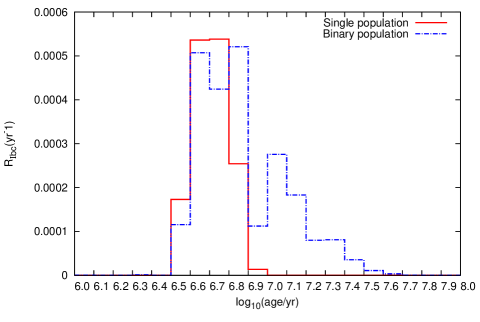
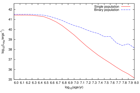
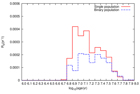
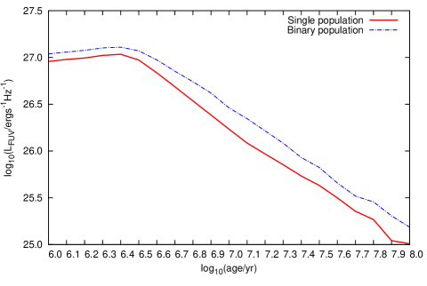
Figure 1: Distributions of CCSN rate in terms of stellar age for type Ibc SNe in the left top panel and for type II SNe in the left bottom panel. The relations of ${\rm H\alpha}$ and FUV flux across stellar age are shown in right top panel and right bottom panel separately. The red solid lines are from single-star model and blue dashed lines are from binary-star model.

3.2 Binary Effect on CCSN Rate and SFRIs

We construct our galaxy model using the results of BPASS, a population-synthesis model based on a detailed stellar evolution code calculated in Eldridge et al. (2008). There are two sets of detailed evolution model, single stars and an extensive set of binary stars, to produce a realistic synthetic stellar population as observations show approximately 70 per cent of massive stars have their evolution affected by binary interactions (e.g. Sana et al., 2012). These evolution models are combined with an atmosphere model to predict emitted spectrum of the stars. Moreover, a composite stellar spectrum is calculated for a range of ages. This process is described in detail in Eldridge & Stanway (2009, 2012).

To calculate the CCSN rate, first we determine whether a star produces CCSN and which types CCSN occur at the end of its evolution. We use the same requirements for both single-star population and binary-star population. A star with final mass greater than 2${\rm M_{\odot}}$ and carbon-oxygen core mass over 1.38${\rm M_{\odot}}$ are taken to experience a CCSN. All the identified CCSN progenitors are then divided into type II SNe with hydrogen in the final model and type Ibc SNe without hydrogen. Therefore, the fate of a star at given initial mass is determined by its mass loss during its lifetime. Compared to single-star model, mass transfer in an interacting binary systems can remove the outer hydrogen envelope from a star’s surface and also lead to mass gain from the companion star. This result is a difference in the CCSN rate of different types as shown in Figure 1. The predicted rates are from the composite model obtained by mixing the five metallicity populations. For both single-star and binary-star model, type II SNe arise from similar stellar population in terms of stellar age arranging from 6 Myrs to 60 Myrs, because more massive stars that die earlier have strong stellar winds that will remove the hydrogen for both sets of models. The binary model however have a reduced occurrence of type II SNe and increased the probability of type Ibc SNe. In addition, a type Ibc SN progenitor can only occur after a lifetime of 10 Myrs from an interacting binary star. When it comes to the total CCSN rate, binary populations make little difference, but as we have demonstrated it plays an important role in changing the relative ratio of type Ibc to type II SNe.

Interacting binaries also have a great effect on both ${\rm H\alpha}$ and FUV fluxes. Although the effect diverges with age. The ${\rm H\alpha}$ line from a star-forming galaxy is produced by hydrogen gas that have been photonionized by hot massive stars. This emission is contributed by stars with stellar ages less than 16 Myrs (Kennicutt, 1998; Gogarten et al., 2009). Therefore, we derived ${\rm H\alpha}$ luminosity by taking account of all the Lyman continuum photons ${\rm N(LyC)}$ below the wavelength of ${\rm\lambda=912\mathring{A}}$ and follow the hydrogen recombination relation provided by Osterbrock & Ferland (2006):

$$L(H\alpha)=1.36\times 10^{-12}N({\rm LyC})\,{\rm erg\,s^{-1}}$$ (2)

While the FUV flux arises from the continuum spectrum at the wavelength between ${\rm 1556\mathring{A}}$ to ${\rm 1576\mathring{A}}$ directly from the stars themselves spectrum. Stars contribute to this with ages up to approximately 100 Myrs (Kennicutt, 1998; Gogarten et al., 2009).

How the ${\rm H\alpha}$ and FUV fluxes vary with stellar age of our composite metallicity population are shown in the right two panels of Figure 1. We see that the binary-star population produces more flux than single-star population. These are in agreement with the greater values predicted by Zheng et al. (2012). The extra emission occurs because of the binary interactions creating more hot stars with their hydrogen envelope stripped and mass-gain in binary systems. The FUV fluxes follow each other with the binary populations being only 0.1 to 0.2 dex greater at any age.

A greater difference occurs for the ${\rm H\alpha}$ flux. After 3 Myrs which is the life duration of a typical H II region (Crowther, 2013), the ${\rm H\alpha}$ flux from binary-star model does not decay as rapidly as single-star model. This again is due to more longer-lived stars but also more hot massive stars at later times to continue to contribute to the ${\rm H\alpha}$ flux. In addition, the short lifetime of the typical H II region implies that binary-star models have only a small effect on observed H II regions. However over longer timescale the amount of diffuse ${\rm H\alpha}$ emission from a galaxy might represent less star-formation than previously thought.

3.3 Our Synthetic 11HUGS Model

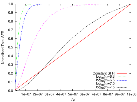
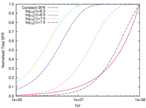
Figure 2: Delayed SFR as a function of time under 4 different time scale parameter with logarithm value of 6.3, 6.5, 7.0 ,7.5 respectively, and compare with constant SFH in red solid lines. The right panel is in linear time scale and the left panel is in logarithm time scale.

Using the BPASS results described above, we construct our synthetic 11HUGS galaxies model as follows. We follow the method of Eldridge (2012) by creating galaxies from individual star clusters from a range of masses between 50${\rm M_{\odot}}$ and ${\rm 10^{6}M_{\odot}}$. We pick the masses at random according to a cluster mass function from Hunter et al. (2003) of the form:

$$\frac{dN}{dM}\propto M^{-2}$$ (3)

Rather than uniformly distributing the age of clusters we set their age randomly too. For example to reproduce a constant star formation we allow the cluster to have any age from 0 to 10 Gyrs ago. With each cluster’s age and mass we then select and scale the appropriate BPASS output and add it into our total predicted spectrum and current CCSN rate of model galaxies. After repeated work as above for different metallicity galaxy populations we mix the model galaxies based on the metallicity classification of 11HUGS sample and obtain a composite 11 HUGS model. With this method of creation we have a prediction of SFRIs appearance and CCSN rate from stellar populations spanning a SFR from ${\rm 10^{-3}M_{\odot}yr^{-1}}$ to ${\rm 100M_{\odot}yr^{-1}}$. At low SFRs our results do predict a range of possible appearances due to stochastic effects which can be seen in Table 4 (e.g. Pflamm-Altenburg et al., 2009; Fumagalli et al., 2011; Eldridge, 2012; Weisz et al., 2012), however in the amount of SFR of the 11HUGS sample are at a level beyond stochastic effects.

A further variation to our 11HUGS model is that we have also created models with a delayed SFH as in Lee et al. (2010). The SFR, $\Psi(t,\tau)$, in the delayed SFH is given by

$$\Psi(t,\tau)\propto\frac{t}{\tau^{2}}e^{-t/\tau}$$ (4)

where t is the time since the onset of star formation and ${\rm\tau}$ is the star formation time scale parameter. In our work we allow ${\rm\tau}$ to vary from 1 Myrs to 30 Myrs. Compared to constant SFH, delayed SFH has its dominated star-burst time range around ${\rm\tau}$ where we can expect relatively high SFR appears. This time range is directly dependent on the choice of ${\rm\tau}$. Increasing ${\rm\tau}$ increases the proportion of older stars relative to the younger stars, and therefore alters the predicted results of our synthetic models. As shown in Figure 2, SFH with lower values of ${\rm\tau}$ experience a sharper increase at earlier times. As ${\rm\tau}$ increases, delayed SFH approach to constant SFH evolving similarly. From the plot in logarithm time scale, we can have a more clearly look at its dominated star-burst period. Here, the position with the largest increasing slope correspond to a star-burst peak which is around ${\rm\tau}$. After the peak SFH decline gradually and a lower value of ${\rm\tau}$ speed up this decline. As s result, increasing the value of ${\rm\tau}$ does not only delay the star-burst peak time, but also extend the duration of the star formation. Moreover, we can associate our predicted CCSN rate to a stellar population with its dominated star-burst period known.

Our synthetic galaxy models under a delayed SFH and constant SFH predicting CCSN rate and full synthetic spectrum can be compared directly to the observed 11HUGS galaxies.

4 Comparison With 11HUGS

4.1 Constant SFH Model

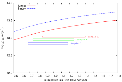
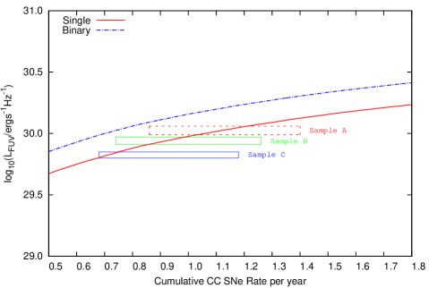
Figure 3: Constant star foramtion model: ${\rm H\alpha}$ and FUV flux as a function of cummulative CCSN rate. The red solid lines are from single-star model and blue dashed lines are from binary-star model. The colored boxes show the observed flux and CCSN rate of Sample A, B, C as shown in Table 1. Since the FUV flux of Sample A is arichived from our estimation, we mark it in a dashed red box.

Table 6: Relative ratio of type Ibc SNe to type II SNe (${\rm R_{Ibc}/R_{II}}$) under constant SFH.

*	${\rm R_{Ibc}/R_{II}}$
Observed ratio	$0.31\pm 0.18$
Z	single	binary	Mix single & binary
0.001	0.002	0.45	0.23
0.004	0.07	0.63	0.35
0.008	0.10	0.60	0.35
0.020	0.20	0.65	0.42
0.040	0.23	0.72	0.48
Mixed Z	0.22	0.70	0.46

Our constant SFH model is the simplest case to consider. We show how the ${\rm H\alpha}$ and FUV fluxes vary relative to the CCSN rate in Figure 3. The values expected for the 11HUGS galaxies are shown by the boxes indicating the range of values allowed for the observed fluxes and CCSN rates. We find both single-star and binary-star models perform reasonably well with predictions within a factor of 2 to the observed values. Also the agreement is closer for the FUV flux rather than the ${\rm H\alpha}$ flux. However the models tend to overestimate the amount of ${\rm H\alpha}$ and FUV fluxes required to reproduce the observed CCSN rate, showing there is a possible excess of CCSNe as found by several studies (e.g. Ando et al., 2005; Kistler et al., 2011; Mattila et al., 2012; Horiuchi et al., 2013). We also find that the standard single-star population achieves the closest fit to the observed parameters. Our binary-star models produce much greater ${\rm H\alpha}$ flux than the single-star population which causes tension with the observations. However there are limitations to our models which currently do not yet account for the effects of dust on the ${\rm H\alpha}$ and FUV emission.

On the other hand there is another test we can apply as shown in Table 6. The ratio of the rate of type Ibc SNe to the rate of type II SNe is $0.31\pm 0.18$. The large error is due to the small number of events. This ratio is strongly dependent on age, interacting binary fraction and metallicity. The effect of the latter is shown in Table 6. The predicted CCSN rate ratios for our single-star and binary-star models are either side of the observed value. The single-star prediction is lower than the observed value but within the range allowed by errors. By contrast, the ratio from binary stars is higher than the observed value. However a mix of single-star and binary-star population also gives a good fit to the observed value.

4.2 Delayed SFH Model

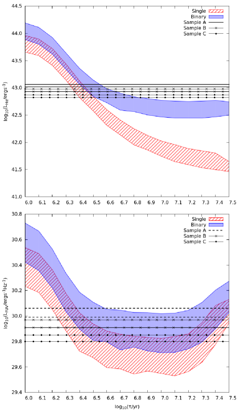
Figure 4: Delayed SFH model: ${\rm H\alpha}$ and UV flux as a function of timescale parameter $\tau$. The shaded regions show the range of ${\rm H\alpha}$ and FUV flux when the predicted CCSN rate matches the observed rate of the 11HUGS galaxies in Table 1. The pairs of black straight lines show the observed value range of ${\rm H\alpha}$ and UV flux in Sample A，B and C as shown in Table 1. Because the FUV flux of Sample A is arichived from our estimation, we mark it by two dashed black lines.

With constant SFH we predict too much ${\rm H\alpha}$ and FUV flux relative to the CCSN rate. We therefore decided to investigate alternative SFHs in order to reduce the contribution of young stars. A delayed SFH is applied as described in Section 3. The outcomes we achieve under the delayed star birth assumption are shown in Figure 4. Here the shaded regions show the range of ${\rm H\alpha}$ and FUV fluxes from our synthetic galaxies in which the predicted CCSN rate matches the observed rate of the 11HUGS galaxies.We see that for matching the ${\rm H\alpha}$ flux and the CCSN rate at the same time the preferred values for $\log(\tau)$ are between 6.3 to 6.7, or times of 2 to 5 Myrs. Although the binary-star models are only just below the observed values and so longer values of $\tau$ would not be unreasonable. While to match the FUV flux and CCSN rate a much wider range of possible values for $\log(\tau)$ are possible between 6.3 to 7.4, or times of 2 to 25 Myrs. This implies that FUV flux follows on a much longer timescale than the ${\rm H\alpha}$ flux as expected.

Figure 5 illustrates how the relative ratio of the two CCSN type rates, ${\rm R_{Ibc}/R_{II}}$, varies with $\tau$. This plot is similar to Figure 4 showing that as $\tau$ increases the binary-star models are favoured relative to the single-star models where the ratio drops for the single stars. The key difference between the single-star and binary-star models is that the single-star population can only reproduce the observation for $\tau$ in a short period of approximately 2 Myrs. While the binary population, or a mix of single stars and binaries could reproduce the 11HUGS observations over a much longer time scale. However the delayed SFH models are in effect just a starburst model where the age of the burst is linked to its duration. So the best fit we can rule out is that the SFH that best matches the 11HUGS galaxies is one that is not dominated by a recent young burst but older more mature bursts.

In summary, our delayed SFH models show a preference for 3 Myrs in matching with observed values. This fact could be due to a sample selection effect but this is remote as 11HUGS are a distance limited sample not ${\rm H\alpha}$ selected. It is more likely that we are over predicting the ${\rm H\alpha}$ emission over the first 3 Myrs of the star formation.

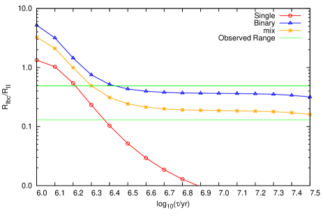
Figure 5: The relative ratio of type Ibc SNe and type II SNe (${\rm R_{Ibc}/R_{II}}$) as a function of timescale paparamter $\tau$. The red dotted line is from sinlge-star model and blue dotted line is from binary-star model. A mixed population of single-star and binary-star model is shown in the yellow dotted line. The green horizontal lines show the observed CCSN ratio range ($0.31\pm 0.18$) as shown in Table 6.

5 Discussion & Conclusions

We have created a synthetic model of the 11HUGS galaxies to investigate the effect of interacting binary stars. We find binaries do not vary the overall CCSN rate to any great degree but do boost the number of type Ibc SNe and the ${\rm H\alpha}$ and FUV SFRIs linked to hottest stars.

In trying to match the observations of the 11HUGS galaxies we must discuss the caveats within our population models. We have not yet accounted for the absorption of the ionizing photons by dust grains and therefore these photons do not form ${\rm H\alpha}$ flux (e.g. Relaño et al., 2012). This effect is not yet included in our models. In addition, the 11HUGS samples are only nearly complete. As in Sample A there is more star formation occurring than in Sample B, the expected Sample A FUV flux might be greater than we predict here. This result would then be in closer agreement with the binary-star population under constant SFH model. Therefore we should not be too surprised that the match is not perfect but there is more work to refine the synthetic galaxy population.

The most surprising fact however is that our constant SFH models produce too many CCSNe in the nearest 11 Mpc of space as argued in Horiuchi et al. (2013). This implies that all supernovae predicted by the models have to be observed. If some massive stars form black holes at core collapse and are unobservable event as suggested by Horiuchi et al. (2014) then this excess of stellar deaths compared to stellar population models becomes more severe. However estimating whether a specific stellar model would produce an observable SN or not requires detailed modelling of the core-collapse and the subsequent explosion.

On the other hand, the delayed SFH model argues that the predicted CCSN rate from ${\rm H\alpha}$ and FUV SFRIs is dependent on the assumption of the SFH. One interpretation of our preferred delayed SFH model is that it implies we over estimate the flux from young stars and therefore get an excess of CCSNe. A similar result is also provided by ionizing photon leakage and dust attenuation on ${\rm H\alpha}$ and FUV flux. Therefore to truly determine if the SFRIs and CCSN rate match, the ionized photon leakage and dust attenuation must be considered. However this is not straightforward.

We have also investigated how sensitive our results are to the metallicity calibration we use for modelling the metallicities of the 11HUGS galaxies. We find that having the more metal rich biased population leads to small changes in the ${\rm H\alpha}$ and FUV fluxes. With a more metal poor distribution we would find even more ${\rm H\alpha}$ and FUV fluxes and would result in greater disagreement between the observations and our models. Therefore the mismatch between our constant star-formation models and observations is difficult to explain by an incorrect metallicity distribution.

Our main conclusion is that single-star models matches the observations best in terms of the prediction of total CCSN rate, when the effects of ionizing photon leakage and dust attenuation are not considered and assuming the local star formation has followed a constant SFH over the last few 100 Myrs. Binary-star models however prolong the stellar age of stars to go CCSN and therefore provide a better prediction of CCSN rate under various SFH spanning star-burst duration between 3 and 25 Myrs ago. In addition, single-star models under constant SFH predicted a lower ratio of type Ibc relative to type II SN but still within the observed uncertainty. By contrast, binary-star models overestimate the ratio. However, a mix of single-star and binary-star model also gives a good fit as in Eldridge et al. (2008, 2013). The limitation in making a firm determination is due to the large uncertainty caused by limited numbers of CCSN discovered. With more CCSN discovered within 11 Mpc this uncertainty will decrease. If the number of CCSN is doubled we estimate that it may become possible to rule out the single-star only population. One final argument against the single-star model is that under the delayed SFH the single-star model only match the observations for a burst of star formation only 2 Myrs old. However mixing in binaries to the single-star population provides a better fit with weaker constraints on the age of the population.

Finally we note that our results are robust if the CCSN sample is complete. However we already obtain too many CCSNe compared to its associated ${\rm H\alpha}$ and FUV. If there are missing SNe or other massive stellar deaths in our sample that are not included in our CCSN sample then the disagreement between models and observations becomes worse with too many stars dying compared to the number we observe forming.

References

- Anderson et al. (2012) Anderson, J. P., Habergham, S. M., James, P. A., & Hamuy, M. 2012, MNRAS, 424, 1372
- Ando et al. (2005) Ando, S., Beacom, J. F., Y& uumlksel, H. 2005, Physical Review Letters, 95, 171101
- Barbon et al. (2008) Barbon, R., Buondi, V., Cappellaro, E., & Turatto, M. 2008, VizieR Online Data Catalog, 1, 2024
- Bersten et al. (2014) Bersten, M. C., Benvenuto, O. G., Folatelli, G., et al. 2014, AJ, 148, 68
- Boissier & Prantzos (2009) Boissier, S., & Prantzos, N. 2009, A & A, 503, 137
- Boquien et al. (2015) Boquien, M., Calzetti, D., Aalto, S., et al. 2015, arXiv:1502.01347
- Botticella et al. (2008) Botticella, M. T., Riello, M., Cappellaro, E., et al. 2008, A & A, 479, 49
- Botticella et al. (2012) Botticella, M. T., Smartt, S. J., Kennicutt, R. C., et al. 2012, A&A, 537, A132
- Cao et al. (2013) Cao, Y., Kasliwal, M. M., Arcavi, I., et al. 2013, ApJ, 775, LL7
- Charlot & Fall (2000) Charlot, S., & Fall, S. M. 2000, ApJ, 539, 718
- Crowther (2013) Crowther, P. A. 2013, mnras, 428, 1927
- De Donder & Vanbeveren (1998) De Donder, E., & Vanbeveren, D. 1998, A & A, 333, 557
- de Mink et al. (2013) de Mink, S. E., Langer, N., Izzard, R. G., Sana, H., & de Koter, A. 2013, ApJ, 764, 166
- Ekström et al. (2012) Ekström, S., Georgy, C., Eggenberger, P., et al. 2012, A & A 537, AA146
- Eldridge et al. (2008) Eldridge, J. J., Izzard, R. G., & Tout, C. A. 2008, MNRAS, 384, 1109
- Eldridge & Stanway (2009) Eldridge, J. J., & Stanway, E. R. 2009, MNRAS, 400, 1019
- Eldridge (2012) Eldridge, J. J. 2012, MNRAS, 422, 794
- Eldridge & Stanway (2012) Eldridge, J. J., & Stanway, E. R. 2012, MNRAS, 419, 479
- Eldridge et al. (2013) Eldridge, J. J., Fraser, M., Smartt, S. J., Maund, J. R., & Crockett, R. M. 2013, MNRAS, 436, 774
- Eldridge et al. (2015) Eldridge, J. J., Fraser, M., Maund, J. R., & Smartt, S. J. 2015, MNRAS, 446, 2689
- Filippenko (1997) Filippenko, A. V. 1997, ARA & A, 35, 309
- Fruchter et al. (2006) Fruchter, A. S., Levan, A. J., Strolger, L., et al. 2006, Natur, 441, 463
- Fumagalli et al. (2011) Fumagalli, M., da Silva, R. L., & Krumholz, M. R. 2011, ApJ, 741, LL26
- Gogarten et al. (2009) Gogarten, S. M., Dalcanton, J. J., Williams, B. F., et al. 2009, ApJ, 691, 115
- Hakobyan (2008) Hakobyan, A. A. 2008, Astrophysics, 51, 69
- Horiuchi et al. (2011) Horiuchi, S., Beacom, J. F., Kochanek, C. S., et al. 2011, ApJ, 738, 154
- Horiuchi et al. (2013) Horiuchi, S., Beacom, J. F., Bothwell, M. S., & Thompson, T. A. 2013, ApJ, 769, 113
- Horiuchi et al. (2014) Horiuchi, S., Nakamura, K., Takiwaki, T., Kotake, K., & Tanaka, M. 2014, MNRAS, 445, L99
- Hunter et al. (2003) Hunter, D. A., Elmegreen, B. G., Dupuy, T. J., & Mortonson, M. 2003, AJ, 126, 1836
- James & Anderson (2006) James, P. A., & Anderson, J. P. 2006, A & A, 453, 57
- Kelly et al. (2008) Kelly, P. L., Kirshner, R. P., & Pahre, M. 2008, apj, 687, 1201
- Kennicutt (1998) Kennicutt, R. C., Jr. 1998, ARA&A, 36, 189
- Kewley & Ellison (2008) Kewley, L. J., & Ellison, S. L. 2008, A, 681, 1183
- Kistler et al. (2011) Kistler, M. D., Yüksel, H., Ando, S., Beacom, J. F., & Suzuki, Y. 2011, PhRvD, 83, 123008
- Kobulnicky & Kewley (2004) Kobulnicky, H. A., & Kewley, L. J. 2004, ApJ, 617, 240
- Langer (2012) Langer, N. 2012, ARA & A, 50, 107
- Lee et al. (2004) Lee, J. C., Kennicutt, R. C., Funes, J. G., et al. 2004, Bulletin of the American Astronomical Society, 36, 1442
- Lee et al. (2010) Lee, S.-K., Ferguson, H. C., Somerville, R. S., Wiklind, T., & Giavalisco, M. 2010, ApJ, 725, 1644
- Lee et al. (2011) Lee, J. C., Gil de Paz, A., Kennicutt, R. C., Jr., et al. 2011, ApJS, 192, 6
- Li et al. (2007) Li, W., Wang, X., Van Dyk, S. D., et al. 2007, ApJ, 661, 1013
- Maeder & Meynet (2000) Maeder, A., & Meynet, G. 2000, A & A, 361, 159
- Mattila et al. (2012) Mattila, S., Dahlen, T., Efstathiou, A., et al. 2012, apj, 756, 111
- Melbourne & Salzer (2002) Melbourne, J., & Salzer, J. J. 2002, AJ, 123, 2302
- Osterbrock & Ferland (2006) Osterbrock, D. E., & Ferland, G. J. 2006, Astrophysics of gaseous nebulae and active galactic nuclei, 2nd. ed. by D.E. Osterbrock and G.J. Ferland. Sausalito, CA: University Science Books, 2006
- Pettini & Pagel (2004) Pettini, M., & Pagel, B. E. J. 2004, MNRAS, 348, L59
- Pflamm-Altenburg et al. (2009) Pflamm-Altenburg, J., Weidner, C., & Kroupa, P. 2009, MNRAS, 395, 394
- Podsiadlowski et al. (1992) Podsiadlowski, P., Joss, P. C., & Hsu, J. J. L. 1992, apj, 391, 246
- Relaño et al. (2012) Relaño, M., Kennicutt, R. C., Jr., Eldridge, J. J., Lee, J. C., & Verley, S. 2012, MNRAS, 423, 2933
- Smartt et al. (2009) Smartt, S. J., Eldridge, J. J., Crockett, R. M., & Maund, J. R. 2009, MNRAS, 395, 1409
- Smartt (2009) Smartt, S. J. 2009, ARA&A, 47, 63
- Smartt (2015) Smartt, S. J. 2015, arXiv:1504.02635
- Smith et al. (2011) Smith, N., Li, W., Filippenko, A. V., & Chornock, R. 2011, MNRAS, 412, 1522
- Sana et al. (2012) Sana, H., de Mink, S. E., de Koter, A., et al. 2012, Science, 337, 444
- Tremonti et al. (2004) Tremonti, C. A., Heckman, T. M., Kauffmann, G., et al. 2004, ApJ, 613, 898
- Vanbeveren et al. (1998) Vanbeveren, D., De Loore, C., & Van Rensbergen, W. 1998, A& ARv, 9, 63
- Williams et al. (2014) Williams, B. F., Peterson, S., Murphy, J., et al. 2014, apj, 791, 105
- Weisz et al. (2012) Weisz, D. R., Johnson, B. D., Johnson, L. C., et al. 2012, ApJ, 744, 44
- Zhang & Li (2012) Zhang, R. Y., & Li, Y. 2012, Acta Astronomica Sinica, 53, 274
- Zheng et al. (2012) Zheng, R., Jiang, Y., Yang, J., et al. 2012, A & A, 541, AA49