The Sloan Digital Sky Survey Reverberation Mapping Project: Ensemble Spectroscopic Variability of Quasar Broad Emission Lines

Abstract

We explore the variability of quasars in the Mg ii and $\rm{H}\beta$ broad emission lines and UV/optical continuum emission using the Sloan Digital Sky Survey Reverberation Mapping project (SDSS-RM). This is the largest spectroscopic study of quasar variability to date: our study includes $29$ spectroscopic epochs from SDSS-RM over $6$ months, containing $357$ quasars with Mg ii and $41$ quasars with $\rm{H}\beta$. On longer timescales, the study is also supplemented with two-epoch data from SDSS-I/II. The SDSS-I/II data include an additional $2854$ quasars with Mg ii and $572$ quasars with $\rm{H}\beta$. The Mg ii emission line is significantly variable ($\Delta f/f\sim 10\%$ on $\sim 100$-day timescales), a necessary prerequisite for its use for reverberation mapping studies. The data also confirm that continuum variability increases with timescale and decreases with luminosity, and the continuum light curves are consistent with a damped random-walk model on rest-frame timescales of $\gtrsim 5$ days. We compare the emission-line and continuum variability to investigate the structure of the broad-line region. Broad-line variability shows a shallower increase with timescale compared to the continuum emission, demonstrating that the broad-line transfer function is not a $\delta$-function. $\rm{H}\beta$ is more variable than Mg ii (roughly by a factor of $\sim 1.5$), suggesting different excitation mechanisms, optical depths and/or geometrical configuration for each emission line. The ensemble spectroscopic variability measurements enabled by the SDSS-RM project have important consequences for future studies of reverberation mapping and black hole mass estimation of $1<z<2$ quasars.

1. introduction

Aperiodic luminosity variations across the electromagnetic spectrum are an ubiquitous feature of quasars (for a review, see Ulrich et al., 1997). The optical and ultraviolet (UV) continuum emission of a typical (nonblazar) quasar vary by a few tenths of a magnitude on timescales from weeks to years. Theoretically, the observed quasar continuum variability may be driven by several kinds of complex instabilities in the accretion disk (e.g., Lyubarskii, 1997; Czerny et al., 1999; Czerny, 2006; Li & Cao, 2008; Kelly et al., 2011). Observationally, however, photometric light curves can be well-modeled by a simple stochastic process: the damped random-walk (DRW) model (for the statistical properties of the DRW model, see Section 5.2). The large body of work on both individual and ensemble quasar variability has established that the amplitude of continuum variability increases with time between epochs, decreases with quasar luminosity and rest-frame wavelength, and is independent of redshift (e.g., Uomoto et al., 1976; Hook et al., 1994; Giveon et al., 1999; Hawkins, 2002; Vanden Berk et al., 2004; de Vries et al., 2005; Bauer et al., 2009; Kelly et al., 2009; MacLeod et al., 2012; Zuo et al., 2012).

Quasar broad emission lines arise from doppler-broadened line emission from gas deep within the gravitational potential well of the supermassive black hole, i.e., the broad line region (BLR), that is photoionized by the extreme UV (EUV) accretion disk continuum radiation. As a result, they vary in response to the continuum variations after a light-travel time delay. The amplitude and shape of the emission-line response are governed by the broad-line transfer function (Blandford & McKee, 1982). The transfer function is ultimately determined by the radiative mechanism, as well as the structure, dynamics, and ionization state of the BLR. The variability time delay enables reverberation mapping to study the structure of the BLR (e.g., Gaskell, 2009) and (with assumptions about the geometry and BLR dynamics) estimate the black hole mass (e.g., Peterson, 1993; Laor, 1998; Peterson et al., 1998; Kaspi et al., 2000; Peterson, 2014). In theory, the reverberation mapping technique can be performed using any broad emission lines that respond to the variability of continuum emission. In practice, however, reverberation mapping has been largely restricted to using the $\rm{H}\beta$ emission line in low-luminosity systems at low redshift (e.g., Peterson & Bentz, 2006).

Employing reverberation mapping with optical spectroscopy at $z>1$ is critical for our understanding of the mass growth of supermassive black holes, as most mass growth occurs at this epoch. However, optical reverberation mapping at $z>1$ requires using rest-frame UV broad emission lines, such as Mg ii. Mg ii is ionized by $E>15\ \rm{eV}$ photons (i.e., the ionization energy to go from Mg ii to Mg iii), which is similar to the ionization energy ($E>13.6\ \rm{eV}$) of H i (which subsequently leads to recombination and $\rm{H}\beta$ emission). In addition, the similarity between the Mg ii and $\rm{H}\beta$ velocity widths indicates the two lines are produced in a similar environment and distance from the central black hole (e.g., Shen et al., 2008; Wang et al., 2009; Shen & Liu, 2012). However, the validity of Mg ii as a black-hole mass estimator is under debate. The variability of Mg ii has only been observed in a handful of quasars, and it is not entirely clear that this variability can be robustly traced to coherent reverberation of the ionizing EUV continuum (e.g., Clavel et al., 1991; Reichert et al., 1994; Trevese et al., 2007; Woo, 2008; Hryniewicz et al., 2014; Cackett et al., 2015). Moreover, the radiative mechanism to produce Mg ii may also differ from that for $\rm{H}\beta$, as the former may mostly be collisionally excited while the latter is a recombination line (e.g., MacAlpine, 1972; Netzer, 1980). Therefore, it is vital to investigate the variability of Mg ii for a large sample. This can only be accomplished with a large multi-epoch broad line quasar spectroscopic survey.

In this work, we measure the ensemble variability of broad emission lines and continuum emission using data from the Sloan Digital Sky Survey Reverberation Mapping project (SDSS-RM, Shen et al., 2015a) and from supplemental observations in SDSS-I and SDSS-II. In Section 2 we describe the SDSS observations. Section 3 presents the basic variability of quasar light curves. In Section 4, we present the distribution of the observed luminosity variability. In Section 5, we introduce the structure function as a tool to study quasar variability on different timescales. Section 6 presents the structure function of continuum emission, and Section 7 describes the structure function of Mg ii and $\rm{H}\beta$. In Section 8, we discuss the physical implications of our results. The main results of this work are summarized in Section 9. We adopt a flat $\Lambda$CDM cosmology with $\Omega_{\rm{m}}=0.3$ and $h_{0}=0.7$. Throughout this work, “$\left<x\right>$” and “$\tilde{x}$” represent the arithmetic mean and the median of the variable $x$, respectively.

2. SAMPLE DEFINITION

In this work, we use SDSS data to study quasar variability. The SDSS $2.5$ m telescope is described by Gunn et al. (2006). Eisenstein et al. (2011) give a technical summary of the SDSS-III project, and the SDSS/BOSS spectrograph and reduction pipeline are described by Bolton et al. (2012); Dawson et al. (2013); Smee et al. (2013).

We focus on the data from the SDSS-RM project, which is an ancillary program within SDSS-III and probes the variability of quasars on rest-frame timescales of $1\lesssim\Delta t\lesssim 100\ \rm{days}$. The SDSS-I/II projects provide ancillary data to study the variability of quasars on rest-frame timescales of $100\lesssim\Delta t~{}\lesssim 1000\ \rm{days}$.

2.1. SDSS-RM quasars

The SDSS-RM sample, observed during the SDSS-III BOSS survey (Eisenstein et al., 2011; Dawson et al., 2013), consists of $849$ quasars, each with $32$ epochs of observations (with a total exposure time of $\sim 60$ hours): for technical details, see Shen et al. (2015a). Three out of the $32$ epochs have low S/N spectra (i.e., $\rm{S/N}<0.7\left<\rm{S/N}\right>$) and are rejected. The spectrograph has a wavelength range of $3650$–$10400\ \rm{\AA}$ with a spectral resolution of $R\sim 2000$ (Smee et al., 2013). The flux calibration was performed based on $70$ standard stars at each epoch, using an improved version of the standard BOSS pipeline (for more details, see Shen et al., 2015a).

For each quasar, we fit the quasar spectra and obtained (depending on the observed spectral coverage) $L=\lambda L_{\lambda}$ for rest-frame $\lambda=3000\ \rm{\AA}$ and/or $\lambda=5100\ \rm{\AA}$, as well as the luminosities and the full-width-half-max velocity ($v_{\rm{FWHM}}$) of Mg ii and/or $\rm{H}\beta$. The details of the continuum and the line fitting are described in detail in earlier work (see Shen et al., 2008, 2011).

We then selected a parent sample of $731$ quasars with broad Mg ii or $\rm{H}\beta$ by requiring $z\leq 2.462$. This requirement ensured that either Mg ii or $\rm{H}\beta$ (or both) and their respective continuum regions were present in the BOSS spectrum. We further required that the median $v_{\rm{FWHM}}$ over $29$ epochs $\widetilde{v}_{\rm{FWHM}}>1000\ \rm{km\ s^{-1}}$.

The observed variability is a superposition of the intrinsic variability of quasars, the measurement errors, and the spectrophotometric errors (see Appendix B). We applied the following sample-selection criteria to obtain an unbiased measurement of the intrinsic variability of quasars:

• There are “dropped” epochs where the fiber was not properly plugged into the spectroscopic mask resulting in sudden, unusually large reduction in the spectral flux (Shen et al., 2015a). To avoid these “dropped” spectra, we reject epochs with $\left|m-\tilde{m}\right|>1$, where $m$ is the magnitude at a given epoch and $\tilde{m}$ is the median magnitude over $29$ epochs. About $1\%$ of the total epochs are excluded (roughly consistent with Shen et al., 2015a). Visual inspection shows that this criterion does not reject any cases of real variability.

• There are spectra with low $\rm S/N$ in the $r$-band and therefore with poor flux calibration, since the spectra are calibrated only in $r$-band. To identify these quasars, we reject quasars with $r$-band $\rm S/N$ less than $50$, measured by convolving the spectra with the SDSS $r$-band filter.

• There are spectra that have strong broad-absorption features in their Mg ii profiles. In this case, the measurements of Mg ii flux can be problematic. To avoid this issue, we reject these quasars.

• The observed-frame quasar spectra are dominated by sky lines at wavelengths larger than $9000\ \rm{\AA}$. To avoid this issue, we reject quasars with redshift $z>2.0$ for the $3000\ \rm{\AA}$ continuum and Mg ii and $z>0.8$ for the $5100\ \rm{\AA}$ continuum and $\rm{H}\beta$.

• There are quasars whose observed variability is dominated by measurement errors rather than intrinsic variability. In this case, the estimated intrinsic variability can be highly biased. To avoid this issue, we reject quasars with median signal-to-noise ratio ($\widetilde{\rm S/N}$) of the continuum or line luminosity $<10$, i.e., $\widetilde{\rm S/N}<10$.

• There are two sources with nearby (angular distance $<5^{{}^{\prime\prime}}$, using the SDSS imaging) bright foreground object that contaminate the quasar spectra in some epochs and introduce artificial flux variations in the fibers. To avoid this issue, we reject these two sources.

The final sample (i.e., clean sample) that passed the selection criteria and will be used for subsequent variability analysis of each continuum and emission-line component is summarized as follows:

• the $3000\ \rm{\AA}$ continuum: $577$ quasars;

• Mg ii broad emission line: $357$ quasars;

• the $5100\ \rm{\AA}$ continuum: $97$ quasars;

• $\rm{H}\beta$ broad emission line: $41$ quasars.

For each quasar in the parent sample, we estimated $L_{\rm Bol}$ using $L_{3000}$ and/or $L_{5100}$. The bolometric correction factor is assumed to be $5$ for $L_{3000}$ and $10$ for $L_{5100}$ (e.g., Richards et al., 2006). If a spectrum covered both $3000\ \rm{\AA}$ and $5100\ \rm{\AA}$ we adopted the $L_{3000}$ estimator which is less contaminated by host galaxy starlight and therefore provides a less biased measure of quasar luminosity.

We also measured $M_{\rm{BH}}$ using the single-epoch broad-line (Mg ii and/or $\rm{H}\beta$) estimators:

$$\log(\frac{M_{\rm{BH}}}{M_{\odot}})=A+B\log(\frac{\lambda L_{\lambda}}{10^{44}\ \rm{erg\ s^{-1}}})+2\log(\frac{v_{\rm{FWHM}}}{1000\ \rm{km\ s^{-1}}})$$ (1)

For $\rm{H}\beta$, $\lambda=5100\ \rm{\AA}$, $A=6.91$, $B=0.5$ (Vestergaard & Peterson, 2006); for Mg ii, $\lambda=3000\ \rm{\AA}$, $A=6.74$, $B=0.62$ (Shen et al., 2011). The quantities $\lambda L_{\lambda}$ and $v_{\rm{FWHM}}$ are measured from the averages of $29$ epochs. The measurement uncertainties of $\lambda L_{\lambda}$ and $v_{\rm{FWHM}}$ are typically $0.01$ dex and $5\%$, respectively. The uncertainty of $M_{\rm BH}$ is therefore dominated by the intrinsic uncertainty of the estimator, which is $\sim 0.4$ dex (for a recent review, see Shen, 2013). If a spectrum included both Mg ii and $\rm{H}\beta$, we adopted the average $M_{\rm BH}$ (there are $134$ such spectra in the parent samples), following Vestergaard & Osmer (2009). For these sources, the difference of the two $M_{\rm BH}$ estimators has a median value of $-0.12$ dex (i.e., on average, Mg ii estimators give slightly higher $M_{\rm BH}$ than those using $\rm{H}\beta$) and a standard deviation of $0.35$ dex. Only for three sources in the parent samples (but not in the clean samples) are the differences in the two $M_{\rm BH}$ estimators larger than $1$ dex. Two are $z<0.4$ sources and therefore $v_{\rm FWHM}$ of Mg ii is not well constrained; the redshift of the remaining source is $z=0.923$ and therefore $v_{\rm FWHM}$ of $\rm{H}\beta$ is poorly measured.

Figure 1 presents the distributions of the parent sample and the clean sample in the $L_{\rm{Bol}}-M_{\rm{BH}}$ plane for each component. For the $3000\ \rm{\AA}$ continuum and Mg ii, the clean samples and the parent samples share similar parameter space. However, the clean $5100\ \rm{\AA}$ continuum and $\rm{H}\beta$ samples cover only the low-luminosity and small $M_{\rm BH}$ portion of parameter space, compared to the parent samples. This result is due to the fact that we can only measure the $5100\ \rm{\AA}$ continuum and $\rm{H}\beta$ for $z<0.8$ sources and low-redshift sources are more likely to be less luminous, on average, for a flux-limited survey.

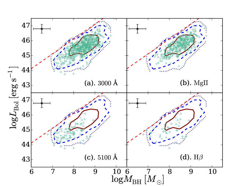
Figure 1.— The distribution of the parent sample of SDSS-RM sources in the $L_{\rm{Bol}}-M_{\rm{BH}}$ plane. The solid, dashed and dotted contours in each panel show boundaries of regions containing $68.2\%$, $95.4\%$ and $99.7\%$ of the total number of sources in our parent SDSS-RM sample. Points in each panel represent the SDSS-RM quasars that passed the selection criteria (i.e., the clean sample). The red dashed line in each panel represents the Eddington luminosity as a function of $M_{\rm BH}$. The error bar in each panel indicates the typical uncertainty of quasar luminosity (due to the uncertainty of the bolometric correction) and $M_{\rm BH}$.

2.2. SDSS-I/II quasars

We use ancillary data compiled from the SDSS-I/II surveys (York et al., 2000) to measure the variability of quasars on longer timescales. This sample includes every quasar with multiple spectroscopic epochs (at least two) in SDSS-I/II. Most of these SDSS-I/II quasars were only observed twice. Only a small fraction of these quasars are observed with SDSS-III. We do not supplement this set of quasars with SDSS-III observations due to the difference in flux calibration from SDSS-I/II to SDSS-III (Margala et al., 2015). We fit the spectra and obtained the luminosities at $\lambda=3000\ \rm{\AA}$ and $\lambda=5100\ \rm{\AA}$ and also the luminosities of the emission lines, Mg ii and $\rm{H}\beta$, following our earlier work (Shen et al., 2008, 2011). For the $3000\ \rm{\AA}$ continuum and Mg ii, a parent sample consisting of $4599$ quasars was compiled. For the $5100\ \rm{\AA}$ continuum and $\rm{H}\beta$, a parent sample with $1347$ quasars was constructed.

To ensure that the intrinsic variability is accurately measured, we applied the fourth and fifth selection criteria described in Section 2.1 to our SDSS-I/II sources. It is not necessary to remove dropped spectra or constrain the $r$-band S/N, since these problems are less frequent in SDSS-I/II spectra (since the spectroscopic flux limit is much shallower). Even if these problems occur in a epoch for a quasar, it only affects a single flux pair (i.e., $f_{2}/f_{1}$) in contrast to SDSS-RM, in which it affects $28$ flux pairs, and we use hundreds to thousands of flux pairs when calculating the variability. The final sample (i.e., clean sample) that passed the selection criteria and will be used for subsequent variability analysis of each continuum and emission-line component is summarized as follows:

• the $3000\ \rm{\AA}$ continuum: $4213$ quasars;

• Mg ii broad emission line: $2844$ quasars;

• the $5100\ \rm{\AA}$ continuum: $1064$ quasars;

• $\rm{H}\beta$ broad emission line: $572$ quasars.

For each quasar in the parent samples, we calculated $M_{\rm{BH}}$ and $L_{\rm Bol}$ following the methods described in Section 2.1. Figure 2 shows the distribution of the SDSSI/II sources in the $L_{\rm{Bol}}-M_{\rm{BH}}$ plane. Three contours again indicate the area that contains $68.27\%$, $95.45\%$ and $99.73\%$ of the parent samples. The points display the distributions of the final samples. For each component, the final sample covers similar parameter space as the parent SDSS-I/II sample. For the $3000\ \rm{\AA}$ continuum and Mg ii, compared to the distribution of final SDSS-RM sources considered, most of the final SDSS-I/II sources cover a similar parameter space. For the $5100\ \rm{\AA}$ continuum and $\rm{H}\beta$, compared to the distribution of the final SDSS-RM sources, the final SDSS-I/II sources cover the high-luminosity and large $M_{\rm BH}$ parameter space. Our analysis treats the SDSS-RM and SDSS-I/II datasets independently, rather than combining the two datasets. This approach was adopted also because the two datasets have different time resolution and the variability of broad emission lines may be correlated with additional parameters beyond $L_{\rm{Bol}}$ and $M_{\rm{BH}}$.

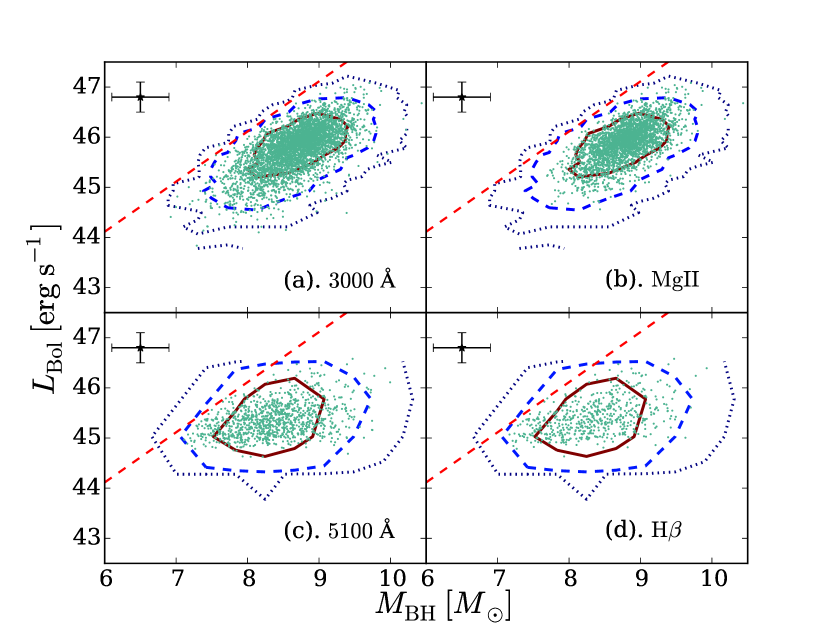
Figure 2.— The distribution of our SDSS-I/II sources in the $L_{\rm{Bol}}-M_{\rm{BH}}$ plane. The solid, dashed and dotted contours in each panel show boundaries of regions containing $68.2\%$, $95.4\%$ and $99.7\%$ of the total number of sources in our initial SDSS-I/II sample. Points in each panel represent the distribution of our final SDSS-I/II sample after applying our selection criteria. The red dashed line in each panel represents the Eddington luminosity as a function of $M_{\rm BH}$. The error bar in each panel indicates the typical uncertainty of quasar luminosity and $M_{\rm BH}$.

3. Light Curve Study

3.1. Observed Light Curves

We start with the basic properties of the observed light curves. Figure 3 plots continuum and broad emission-line light curves of the clean SDSS-RM samples. Throughout this work, we use magnitude (rather than flux or luminosity) changes to characterize variability so that it is straightforward to compare our results with previous photometric studies. The light curves do indicate that there is variability in both continuum emission and broad emission lines. However, the observed variability is a superposition of intrinsic variability, measurement errors, and spectrophotometric errors. The spectrophotometric errors of SDSS-RM for a single epoch are at least $\sim 0.04\ \rm{mag}$, and larger at long and short wavelengths, as computed from standard stars: see Appendix B.1.

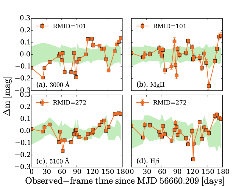
Figure 3.— Continuum and emission-line light curves of typical SDSS-RM sources (red lines/points), and the $25$–$75$ percentile range of the ensemble light curves (green shaded regions). The observed ensemble variability is a few tenths of a magnitude in both the continuum and broad emission lines.

3.2. Basic Light-Curve Variability

Following Sesar et al. (2007), we define the basic intrinsic variability of a light curve with $n$ epochs as,

$$\sigma_{lc}=\sqrt{\frac{1}{n-1}\sum_{i=1}^{n}(m_{i}-\left<m\right>)^{2}-\left<\sigma^{2}_{\rm{e}}\right>)}$$ (2)

where $m_{i}$ is the observed magnitude at each epoch, its corresponding uncertainty is $\sigma_{\rm{e}}$ ($\sigma_{\rm{e}}$ is a summation of measurement errors and spectrophotometric errors in quadrature), and $\left<m\right>$ is the mean magnitude across all epochs. $\sigma_{lc}$ is set to zero if the operand within the square root is less than zero (the fraction of such sources is less than $10\%$). This is motivated by the fact that the variance of the quasar variability is $\geq 0$. The median ratios between the observed variance and the variance due to error (measurement and spectrophotometric), $\frac{1}{n-1}\sum_{i=1}^{n}(m_{i}-\left<m\right>)^{2}/\left<\sigma^{2}_{\rm{e}}\right>$, is $5.6$ for the $3000\ \rm{\AA}$ continuum, $2.5$ for Mg ii, and $2.9$ for $\rm{H}\beta$. Note that we required $\widetilde{\rm S/N}\geq 10$ to ensure that, in most cases, the measurement errors do not dominate the observed variances.

3.2.1 The $3000$ $\rm{\AA}$ Continuum

We first present the variability of the $3000\ \rm{\AA}$ continuum as a function of quasar luminosity (Figure 4). We tested the correlation between the light-curve variability and $L_{\rm{Bol}}$ using the Spearman rank correlation test. The null hypothesis of this test is that there is no correlation between the input datasets. The correlation coefficient of this test is $\rho=-0.44$. The $p$ value (i.e., the probability of being incorrect in rejecting the null hypothesis) is only $5\times 10^{-29}$. Therefore, we conclude that there is a significant anti-correlation between the light-curve variability and quasar luminosity at significance level of $\alpha=0.01$ (i.e., the probability threshold below which the null hypothesis will be rejected). As we show in Section 6, this anti-correlation is not simply due to more luminous quasars having smaller $\sigma_{\rm e}$ or typically being at higher redshift (sampling shorter rest-frame timescales). This behavior is consistent with previous work based on broad-band photometric data (e.g., Vanden Berk et al., 2004; de Vries et al., 2005; Bauer et al., 2009; MacLeod et al., 2012).

Previous work suggests that the Eddington ratio, which depends on both quasar luminosity and $M_{\rm BH}$, is the main driver of quasar continuum variability (e.g., Wilhite et al., 2008; Bauer et al., 2009; Ai et al., 2010; MacLeod et al., 2010). We verify this scenario by testing the possible correlation between the light-curve variability of the $3000\ \rm{\AA}$ continuum and the Eddington ratio. We stress that the uncertainty of the Eddington ratio is rather large since both quasar luminosity and $M_{\rm BH}$ are uncertain by a factor of $\sim 3$. The Spearman correlation coefficient of this test is $\rho=-0.2$ and the $p$ value is $5\times 10^{-7}$. This anti-correlation is consistent with previous work.

Figure 4.— The light-curve variability of the $3000\ \rm{\AA}$ continuum. Each point represents a quasar. The solid, dashed, and dotted lines represent $1\sigma$, $2\sigma$ and $3\sigma$ bounds of the quasar number distribution. The color indicates the probability density of each point (calculated via kernel density estimation). The light curve variability decreases with quasar luminosity. In this figure and Figures 5-9, the error bars indicate the median uncertainty of the light-curve variability.

3.2.2 Mg ii

We explore the variability of the light curve of Mg ii as a function of quasar luminosity (Figure 5). With the same Spearman correlation test, for Mg ii, $\rho=-0.24$ and the $p$ value is $3\times 10^{-6}$. Therefore, again there is an anti-correlation between the light-curve variability of Mg ii and quasar luminosity. The same Spearman correlation test also suggests that the light-curve variability of the Mg ii and the Eddington ratio are anti-correlated (with $\rho=-0.24$, and the $p$ value is $7\times 10^{-6}$). As we show in Section 6, these anti-correlations are not simply due to more luminous quasars preferentially having smaller $\sigma_{\rm e}$ or lying at higher redshift (with shorter rest-frame timescales).

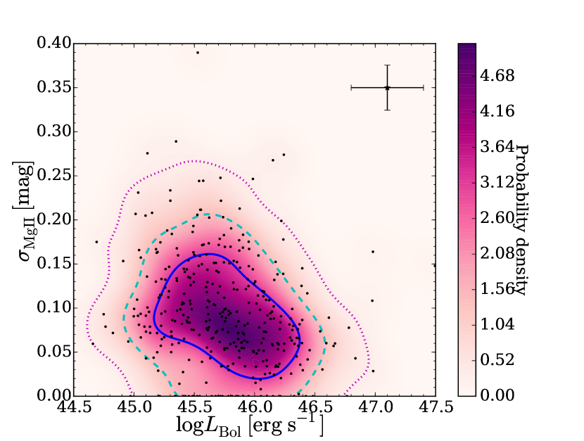
Figure 5.— The light-curve variability of Mg ii. Each point represents a quasar. The solid, dashed, and dotted lines represent $1\sigma$, $2\sigma$ and $3\sigma$ bounds of the quasar number distribution. The color indicates the probability density of each point. The light curve variability of Mg ii also decreases with quasar luminosity.

We compare the light-curve variability of Mg ii with that of the $3000\ \rm{\AA}$ continuum in the left panel of Figure 6. The Spearman correlation test again reveals $\rho=0.62$ and the $p$ value is $6\times 10^{-39}$, i.e., our data favor a significant positive correlation between the light curve variability of Mg ii and that of the $3000\ \rm{\AA}$ continuum. This correlation indicates that the variability in the light curve of Mg ii and that of the $3000\ \rm{\AA}$ continuum are connected. The simplest explanation is that Mg ii varies in response to the $3000\ \rm{\AA}$ continuum (see the cross correlation analysis of Shen et al., 2015c). Furthermore, the scatter in the correlation (for instance, a few sources show significant variability in the $3000\ \rm{\AA}$ continuum but the variability of Mg ii is consistent with $0$) suggests that the response process may not be uniform in all quasars, e.g., the response of the emission line to the continuum and/or the structure of the BLR may differ in different quasars.

In the right panel of Figure 6, we plot the difference between the light curve variability of the $3000\ \rm{\AA}$ continuum and that of Mg ii versus quasar luminosity. Most quasars vary slightly more in the $3000\ \rm{\AA}$ continuum than in the Mg ii line; the median $\sigma_{lc,3000}-\sigma_{lc,\rm{MgII}}$ is $0.003\ \rm{mag}$. A Spearman rank correlation test between the difference in the $3000\ \rm{\AA}$ continuum and Mg ii variability and $L_{\rm Bol}$ indicates that the difference is anti-correlated with quasar luminosity, with $\rho=-0.2$ and a $p$ value of $10^{-4}$; as quasar luminosity increases, the variability of the $3000\ \rm{\AA}$ continuum decreases more rapidly than the Mg ii variability.

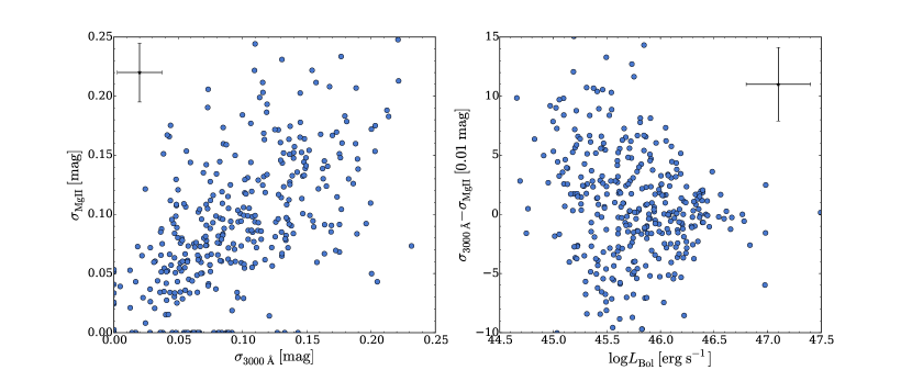
Figure 6.— Left: The light-curve variability of Mg ii against that of the $3000\ \rm{\AA}$ continuum. The light-curve variability of the two components are correlated. Right: The difference between the light-curve variability of the $3000\ \rm{\AA}$ continuum and that of Mg ii. The difference is anti-correlated with quasar luminosity.

3.2.3 $\rm{H}\beta$

We then present the light-curve variability of $\rm{H}\beta$. Since our final sample of $\rm{H}\beta$ consists of only $41$ quasars, we interpret our data with caution.

Figure 7 shows the light-curve variability of $\rm{H}\beta$ as a function of quasar luminosity. The Spearman correlation test suggests that there is no significant correlation between the variability and quasar luminosity ($\rho=-0.09$ with the $p$ value of $0.58$). This result may be due to the small size of our sample. We test such small-sample effects by randomly selecting $41$ quasars from the Mg ii clean sample and testing the correlation between the Mg ii light-curve variability and quasar luminosity. We repeated this simulation $10^{4}$ times and found that $\sim 15\%$ of the time, the anti-correlation between Mg ii variability and quasar luminosity of the limited sample is as weak as or weaker than the Spearman correlation test for $\rm{H}\beta$ variability with quasar luminosity. From this simulation, we conclude that the lack of the correlation between the variability of $\rm{H}\beta$ and quasar luminosity is plausibly caused by the small sample size. We then tested the correlation between the light-curve variability of $\rm{H}\beta$ and the Eddington ratio ($\rho=-0.33$, and the $p$ value is $0.035$) and found the anti-correlation is not statistically significant. We performed the same simulation and found that the lack of correlation is again plausibly due to the small sample size.

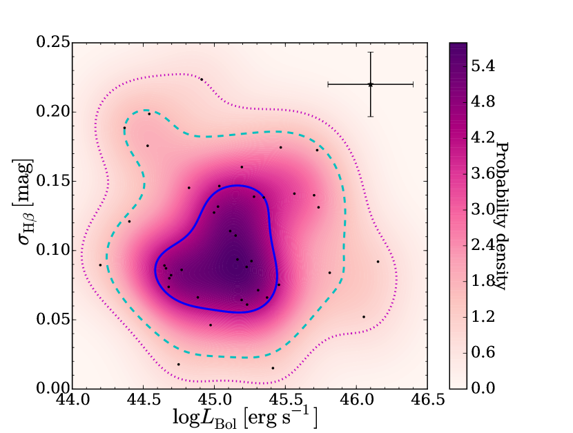
Figure 7.— The light-curve variability of $\rm{H}\beta$. Each point represents a quasar. The solid, dashed, and dotted lines represent $1\sigma$, $2\sigma$ and $3\sigma$ bounds of the quasar number distribution. The color indicates the probability density of each point. The light-curve variability of $\rm{H}\beta$ does not demonstrably depend on quasar luminosity which may due to the fact that there are only $41$ quasars in the sample.

We then compare the light-curve variability of $\rm{H}\beta$ with that of the $3000\ \rm{\AA}$ continuum. We prefer the $3000\ \rm{\AA}$ continuum instead of the $5100\ \rm{\AA}$ continuum because the galaxy contamination to the $5100\ \rm{\AA}$ continuum is more significant (and galaxy contamination biases the observed variability, see Section 6.2). We can only compare quasars for which $\rm{H}\beta$ and the $3000\ \rm{\AA}$ continuum were both observed in the BOSS spectrum ($35$ quasars). The left panel of Figure 8 presents the light curve variability of $\rm{H}\beta$ as a function of that of the $3000\ \rm{\AA}$ continuum. The Spearman correlation test indicates that there is no significant correlation between the variability of $\rm{H}\beta$ and that of the $3000\ \rm{\AA}$ continuum ($\rho=0.28$, and the $p$ value is $0.1$). Once again, we test if the lack of correlation is caused by small sample size by testing for correlations in random subsets of $35$ quasars from the Mg ii clean sample. In $10^{4}$ simulations, the Mg ii and continuum variability are uncorrelated $\sim 0.5\%$ of the time. From this we conclude that the lack of correlation between $\rm{H}\beta$ and continuum variability is not solely due to selection effects. Given the fact that previous reverberation mapping work reveals that $\rm{H}\beta$ does respond to continuum variability, our results indicate that $\rm{H}\beta$ and Mg ii variability relate to continuum variability in different ways. For example, the intrinsic correlation between the $\rm{H}\beta$ variability and continuum variability might be slightly weaker. It is also possible that the transfer function of $\rm{H}\beta$ increases significantly with quasar luminosity, thus making the $\rm{H}\beta$ variability behave opposite to continuum variability as a function of quasar luminosity. The different relationships of $\rm{H}\beta$ and Mg ii variability with quasar luminosity in turn probe the differences between the BLR gas responsible for each line (see Section 8.3).

In the right panel of Figure 8, we plot the difference between the variability of the $3000\ \rm{\AA}$ continuum and that of $\rm{H}\beta$ as a function of quasar luminosity. We again tested the correlation between the difference of the variability and quasar luminosity using the Spearman correlation test. We found that there is an anti-correlation between the differences of the variability and quasar luminosity ($\rho=-0.56$, and the $p$ value is $4\times 10^{-4}$). This correlation makes sense given the previously-found anti-correlation of the $3000\ \rm{\AA}$ continuum variability with quasar luminosity, even with the lack of correlation of $\rm{H}\beta$ variability with quasar luminosity.

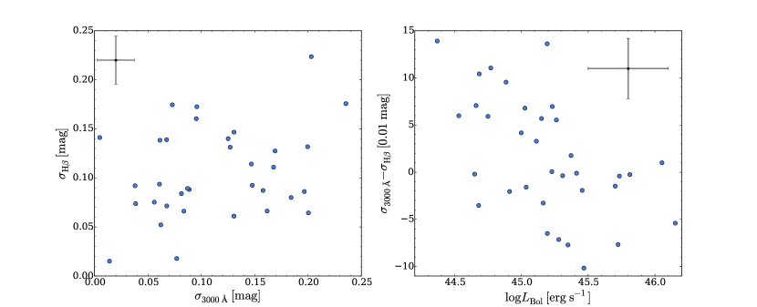
Figure 8.— Left: The light-curve variability of $\rm{H}\beta$ against that of the $3000\ \rm{\AA}$ continuum. There is no significant correlation between the variability of the two components. Right: The difference between the light-curve variability of the $3000\ \rm{\AA}$ continuum and that of $\rm{H}\beta$. The difference is anti-correlated with quasar luminosity.

We performed similar comparisons between $\rm{H}\beta$ and Mg ii. Our results are presented in Figure 9. Again, we can only consider quasars for which Mg ii and $\rm{H}\beta$ were both observed in the BOSS spectrum ($26$ quasars). The Spearman correlation test suggests that there is no strong correlation between the variability of $\rm{H}\beta$ and that of Mg ii ($\rho=0.36$, and the $p$ value is $0.07$), and on average, the variability observed in Mg ii is less than observed for $\rm{H}\beta$. Note that there are seven out of $26$ sources that show significant variability in the light curve of $\rm{H}\beta$ but not in that of Mg ii. This is probably due to the fact that, as Mg ii is on average less variable than $\rm{H}\beta$, the observed light-curve variability of Mg ii is more likely to be dominated by measurement and spectrophotometric errors. The lack of correlation between $\rm{H}\beta$ and Mg ii variaiblity is likely due to the small sample size and/or the differences between the BLR gas that produce $\rm{H}\beta$ and Mg ii (see Section 8.3).

There might be a weak correlation between the difference of the variability of $\rm{H}\beta$ and that of Mg ii and quasar luminosity as revealed by the Spearman test ($\rho=0.51$, and the $p$ value is $0.008$) although the Kendall test suggests that we cannot rule out the no-correlation hypothesis (the $p$ value is $0.02$). This correlation, if indeed exist, can also be explained by the anti-correlation between the variability of Mg ii and quasar luminosity (which holds even we only consider these $26$ quasars), even with the lack of correlation of $\rm{H}\beta$ variability with quasar luminosity.

Figure 9.— Left: The light-curve variability of $\rm{H}\beta$ against that of Mg ii. There is no significant correlation between the variability of the two components. Right: The difference between the light-curve variability of $\rm{H}\beta$ and that of Mg ii. The difference is weakly correlated with quasar luminosity.

4. Observed Distribution of $\Delta m$

Previous studies have revealed that, in general, intrinsic quasar variability is not consistent with white noise but is actually a red-noise process where quasars are more variable on longer timescales (e.g., MacLeod et al., 2010, hereafter M10). The basic light-curve variability we presented in Section 3 is averaged over different timescales.

Before we calculate the quasar variability as a function of rest-frame $\Delta t$ (i.e., the structure function), we first present the distribution of luminosity variability for two different $\Delta t$ bins. We calculated $\Delta m=-2.5\log(f_{2}/f_{1})$ for all luminosity pairs separated by $\Delta t$. The histograms of $\Delta m$ for the continuum and broad emission lines are presented in Figure 10. Note that the observed histograms are a superposition of the intrinsic variability, measurement errors, and spectrophotometric errors (see Appendix B). The distribution of $\Delta m$ is not Gaussian for any component. Actually, the distributions are better described by the Laplace (i.e., double-exponential) distribution. This can be explained either by the fact that the spectrophotometric errors are not Gaussian (see Appendix B) or, as illustrated by MacLeod et al. (2012) (their Section 3.2.2), as natural results of a superposition of many Gaussian distributions.

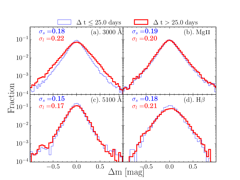
Figure 10.— The histograms of observed $\Delta m$ of the SDSS-RM sources. In this figure, $\Delta m=-2.5\log(f_{2}/f_{1})$, where $f_{1}$ and $f_{2}$ are two measurements of flux separated by rest-frame $\Delta t$. The blue and red lines represent the variability of $\Delta t\leq 25\ \rm{days}$ (the median $\Delta t\sim 12\ \rm{days}$ for $L_{3000}$ and Mg ii and $\sim 14\ \rm{days}$ for $L_{5100}$ and $\rm{H}\beta$) and $\Delta t>25\ \rm{days}$ (the median $\Delta t\sim 40\ \rm{days}$ for $L_{3000}$ and Mg ii and $\sim 50\ \rm{days}$ for $L_{5100}$ and $\rm{H}\beta$), respectively. $\sigma_{s}$ and $\sigma_{l}$ in each panel represent the standard deviation of the short and long timescale distributions, respectively. There are exponential tails in the distribution of $\Delta m$. This is likely due to the superposition of the intrinsic quasar variability (which is a superposition of many Gaussian distributions), measurement errors, and spectrophotometric errors.

The distributions of $\Delta m$ for SDSS-I/II sources are shown in Figure 11. The SDSS-I/II distributions are less well-sampled in $\Delta m$ because each quasar only has two epochs, compared to the $29$ epochs of the SDSS-RM sources. In addition, the increase in variability with $\Delta t$ is clearer in Figure 11 because of the larger range of $\Delta t$ in the SDSS-I/II data (which span tens to thousands of days). Otherwise, the SDSS-I/II variability distribution is similar to our SDSS-RM sources, with similar exponential tails.

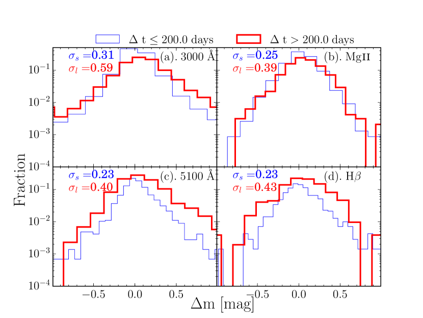
Figure 11.— The histograms of $\Delta m$ of the SDSS-I/II sources. The blue and red lines represent the variability of $\Delta t\leq 200\ \rm{days}$ (the median $\Delta t\sim 20\ \rm{days}$) and $\Delta t>200\ \rm{days}$ (the median $\Delta t\sim 300\ \rm{days}$), respectively. There are exponential tails in the distribution of $\Delta m$. Also, the variability increases with $\Delta t$.

5. The Structure Function: Variability as a Function of Time Separation

In this section, we introduce the structure function, a tool to study quasar variability as a function of rest-frame time separation ($\Delta t$) between observations.

5.1. Definitions

The structure function, $\mathrm{SF}(\Delta t)$, measures the statistical dispersion of observations (e.g., luminosity or flux) separated by time intervals, $\Delta t$. Many non-parametric statistics can be used as estimators of the statistical dispersion of the distribution of $\Delta m$, e.g., the interquartile range (IQR), the median absolute deviation (MAD), the average absolute deviation (AAD), and the standard deviation. The IQR and MAD statistics tend to be more robust against outliers or tails in the distribution than the AAD or standard deviation statistics: see Appendix A for more details. In this work, we adopt the IQR estimator as it has been adopted in previous work. In order to account for the presence of measurement and spectrophotometric errors in our data, we estimate the intrinsic statistical dispersion following MacLeod et al. (2012):

$$\mathrm{SF_{IQR}}(\Delta t)=\sqrt{(0.74\mathrm{IQR}(\Delta m))^{2}-\widetilde{\sigma^{2}_{\rm{e}}}}\,$$ (3)

where $\mathrm{IQR}(\Delta m)$ is the $25\%-75\%$ interquartile range of $\Delta m$ and $\sigma_{\rm{e}}$ is the total uncertainty of $\Delta m$ (i.e., the summation of measurement error and spectrophotometric error in quadrature). The constant $0.74$ normalizes the IQR to be equivalent to the standard deviation of a Gaussian distribution; the IQR is smaller than the standard deviation for a Laplace distribution. Appendix A also includes discussion of alternative structure function estimators: AAD, MAD, and a maximum-likelihood estimator of standard deviation.

The structure function can also be used to characterize the statistical dispersion of $\Delta m$ for a sample of many quasars with the same (or close) $\Delta t$. That is, the ensemble structure function is an average of the structure functions of many sources (as demonstrated by MacLeod et al., 2008, individual and ensemble structure functions result in the same statistical properties). All these structure function estimators involve square roots, and therefore must not be negative. If measurement and spectrophotometric errors are significantly larger than the intrinsic variability of quasars and/or the measurement errors are underestimated by a factor of a few, the ensemble structure function would be strongly biased. Our sample’s $S/N>10$ requirement is designed to minimize this bias.

5.2. The Damped Random-Walk Model

As pointed out by previous work (e.g., Kelly et al., 2009; MacLeod et al., 2012; Zu et al., 2013), the light curves of quasar continuum emission can be well described by the DRW model. The DRW model describes a random process that is characterized by the following covariance matrix:

$$C(x(t_{i}),x(t_{j}))=\mathrm{SF}_{\infty}^{2}\exp(-\Delta t/\tau)/2$$ (4)

where $\Delta t=\left|t_{i}-t_{j}\right|$. $\mathrm{SF}_{\infty}$ and $\tau$ are the asymptotic driving amplitude and the damping timescale. The structure function is given by

$${\mathrm{S}F}(\Delta t|\tau,{\rm SF}_{\infty})={\rm SF}_{\infty}\sqrt{1-\exp(-\Delta t/\tau)}$$ (5)

At $\Delta t\ll\tau$ (with $\tau$ typically on the order of hundreds of days), Eq. 5 can be simplified as,

$$\mathrm{SF}(\Delta t)=\hat{\sigma}\sqrt{\Delta t}$$ (6)

where $\hat{\sigma}=\rm{SF}_{\infty}/\sqrt{\tau}$, and the structure function at $\Delta t=100\ \rm{days}$, $\rm{SF}_{100}=10\hat{\sigma}$. The ensemble structure function for given luminosity, $L$, bin is given by

$$\mathrm{SF_{EN}}(\Delta t)=\int_{\Delta t_{\mathrm{min}}}^{\Delta t_{\mathrm{max}}}\int\int d\Delta t_{0}d\tau dSF_{\infty}\ SF(\Delta t_{0}|\tau,SF_{\infty})$$ (7)

For a quasar, $\tau$ and $\rm{SF}_{\infty}$ (or $\hat{\sigma}$) are determined by $M_{\rm BH}$, $L$, and wavelength (e.g., M10). For a set of quasars binned in a narrow range of $M_{\rm BH}$, $L$, and wavelength, $\tau$ and $\rm{SF}_{\infty}$ (or $\hat{\sigma}$, $\rm{SF}_{100}$) are constant and the integrals above reduce to a simple summation.

6. The Structure Functions of Continuum emission

The main purpose of this work is to investigate the variability of broad emission lines and their connection to the variability of continuum emission. Therefore, we first present the structure function of the continuum emission.

6.1. The $3000$ $\rm{\AA}$ Continuum

In this section, we present the structure function of the $3000\ \mathrm{\AA}$ continuum for the SDSS-RM sources. We first divided our sample into $4$ sub-samples by $L_{\mathrm{Bol}}$: $L_{\mathrm{Bol}}<10^{45.3}\ \mathrm{erg\ s^{-1}}$; $10^{45.3}\ \mathrm{erg\ s^{-1}}\leq L_{\mathrm{Bol}}<10^{45.7}\ \mathrm{erg\ s^{-1}}$; $10^{45.7}\ \mathrm{erg\ s^{-1}}\leq L_{\mathrm{Bol}}<10^{46.1}\ \mathrm{erg\ s^{-1}}$; $L_{\mathrm{Bol}}>10^{46.1}\ \mathrm{erg\ s^{-1}}$. The luminosity bins are constructed to have (roughly) equal numbers of quasars in each. We calculated the ensemble structure function in each bin using the method described in Section 5.1 (subtracting both measurement and spectrophotometric errors). The binned IQR structure functions for the $3000\ \rm{\AA}$ continuum of the SDSS-RM quasars are shown by the solid lines in the left and center panels of Figure 12.

Using a Stripe 82 quasar sample, M10 found that the DRW parameters are correlated with quasar properties in the following way,

$$\log q=Q_{1}+Q_{2}\log(\frac{\lambda_{\mathrm{rf}}}{4000\ \mathrm{\AA}})+Q_{3}(M_{i}+23)+Q_{4}\log(\frac{M_{\mathrm{BH}}}{10^{9}\ M_{\odot}})\\ ,$$ (8)

where for $q=SF_{\infty}$, $Q_{1}=-0.51$, $Q_{2}=-0.479$, $Q_{3}=0.131$, and $Q_{4}=0.18$; for $q=\tau$, $Q_{1}=2.4$, $Q_{2}=0.17$, $Q_{3}=0.03$, and $Q_{4}=0.21$ (here $\tau$ is in units of days). The uncertainty of each coefficient can be found in M10. The intrinsic scatters of the M10 relations are presented in MacLeod et al. (2012). $M_{i}$ is the K-corrected rest-frame $i$-band absolute magnitude.

To compare our results with the M10 relations (i.e., Eq. 8), we performed a simulation based on the M10 relations (hereafter “DRW simulation”). The simulation procedures are similar to those of MacLeod et al. (2012):

1. We calculate a model structure function for each quasar using its $M_{\rm BH}$ and $L_{\rm Bol}$ (translated into rest-frame $M_{i}$ assuming the $i$-band bolometric correction factor is $12$), following Eq. 8. During the calculation, $M_{\rm BH}$, $L_{\rm Bol}$, and the coefficients in Eq. 8 are perturbed by Gaussian noise according to their uncertainties. The predicted $\hat{\sigma}$ (i.e., $SF_{\infty}/\sqrt{\tau}$) and $\tau$ (perturbed by Gaussian noise according to the intrinsic scatter in Eq. 8) are translated into a structure function value at each $\Delta t$ using Eq. 5.

2. In each bin of quasar luminosity at each $\Delta t$, we randomly generated a distribution of $\Delta m$ using the model structure function for each quasar in that bin. We then add the measurement and spectrophotometric errors (following Laplace, not Gaussian, distributions; see Appendix B.1) to create the “observed” variability of the model.

3. We calculated the structure function (using the IQR estimator) from the model distribution of $\Delta m$, subtracting the median errors in quadrature in each bin (see Section 5.1).

By doing this, the simulation includes the same numerical and/or time-sampling issues as the structure function calculated from the real data. We repeated this simulation $256$ times to obtain a simulated structure function for each luminosity bin.

Our results are shown in the left panel of Figure 12 (for other structure-function estimators, see Appendix A). It is evident that the variability amplitude decreases with quasar luminosity and increases with $\Delta t$. Also, the shape of the observed structure function in each luminosity bin can be reproduced well by a simulated DRW model “observed” like the data (i.e., with the same time sampling and measurement/spectrophotometric errors). To verify this, we performed a statistical hypothesis test.

The null hypothesis of our test is the following: for each luminosity bin, the observed structure function and the simulated structure function share the same shape but with different normalization factors (in $\log\mathrm{SF}(\Delta t)-\log\Delta t$ space). We calculated the difference between the observed $\log\mathrm{SF}(\Delta t)$ and the simulated $\log\mathrm{SF}(\Delta t)$ and their uncertainties for each luminosity bin. Note that we only considered data points with $\Delta t>5\ \rm{days}$ (see Section 8.1). If our null hypothesis is true, then the difference we obtained should be, statistically, a constant (i.e., independent of $\Delta t$). We adopted the chi-squared test to assess this hypothesis. For three of the four luminosity bins considered, our data fail to reject the null hypothesis that the two structure functions share the same shape (i.e., the $p$ value of the chi-squared test is $\gg 0.01$). The simulated and observed structure functions have different shapes only in the $10^{45.3}\ \mathrm{erg\ s^{-1}}\leq L_{\mathrm{Bol}}<10^{45.7}\ \mathrm{erg\ s^{-1}}$ bin (although this happens only $25\%$ of the time), but differ in slope by only $\Delta\beta\simeq 0.1$ (parameterizing each by $\mathrm{SF}(\Delta t)\sim\Delta t^{\beta}$).

To characterize the sensitivity of our statistical test, we simulated two pairs of structure functions (both follow $\mathrm{SF}(\Delta t)\sim\Delta t^{\beta}$) with different slopes $\beta$ and with the same S/N as our observed structure functions and our “DRW simulation” structure functions. We then applied our statistical test to each pair of simulated structure functions and calculated the $p$ value of the null hypothesis that the shapes are the same. We repeated this simulation $10^{4}$ times and found that in $80\%$ of the simulations (which is the most widely adopted value in statistical power analysis), our null hypothesis can be rejected if the difference in $\beta$ is $>0.1$ ($>0.2$, for the highest luminosity bin): the difference in slopes is $\lesssim 0.1$. Therefore, we conclude that, for each luminosity bin, the observed structure function and the structure function from our “DRW simulation” share the same shape (the difference in slope $\beta\lesssim 0.1$). That is, as revealed by previous work (e.g., Kelly et al., 2009; MacLeod et al., 2010, 2012), the variability of the quasar continuum emission can be described by the DRW model.

As for the variability amplitude, we find that the M10 relations under-predict the amplitude (by a factor of $\sim 1.3$) except for the highest luminosity bin (i.e., $\log L_{\rm{Bol}}>46.1$). This indicates that while the M10 relations are accurate for high-luminosity quasars, a small revision is required to reproduce the variability of lower luminosity quasars. Note that the quasar sample used in M10 consists of luminous quasars ($M_{i}<-23$) while a significant fraction of quasars in our sample are less luminous ($M_{i}>-23$). That is, our lower-luminosity quasars require extrapolation of the M10 relations, and this extrapolation seems to be inaccurate by a small factor.

In the middle panel of Figure 12, we illustrate the importance of “observing” the model structure function, comparing the “observed” model structure function to the basic model without bias treatment. On long timescales ($\sim 20-100$ days), the two versions of the structure functions are similar. On short timescales ($<20$ days), the two versions of structure function are different and the differences increase with decreasing $\Delta t$. This is because, on short timescales, the uncertainties of our data are comparable to or even dominate over the intrinsic variability, and the bias of the observed structure function is significant. In this case, if we add uncertainties and then subtract them via Eq 3, the model becomes biased toward higher amplitude variability.

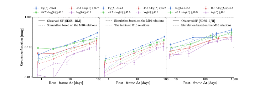
Figure 12.— Left panel: The structure function (solid lines) of the $3000\ \rm{\AA}$ continuum of the SDSS-RM sources for each luminosity bin. The dashed lines represent our simulation results based on the M10 relations “observed” like our data (see the text in Section 6.1). The structure functions increase with $\Delta t$ and decrease with $L_{\rm{Bol}}$. The shapes of the observed structure functions (on timescales $\Delta t>5\ \rm{days}$) are consistent with the DRW model and the M10 relations (the difference in slope $\beta\lesssim 0.1$). The M10 relations slightly under-predict (by a factor of $1.3$) the variability amplitude. Middle Panel: The dotted lines represent the structure functions from the M10 relations without considering the observational bias. On short timescales, the measurement and spectrophotometric uncertainties of our data dominate over the intrinsic quasar variability, and the structure function estimations are biased. The bias is not significant on longer timescales where the intrinsic quasar variability is larger. Right panel: The structure functions (solid lines) of the $3000\ \rm{\AA}$ continuum for SDSS-I/II sources. The dashed lines represent the structure functions predicted by the M10 relations. The M10 relations can roughly reproduce the observed structure functions. According to the M10 relations, for the four luminosity bins, the characteristic timescale $\tau\sim 200\ \rm{days}$. In this figure and the rest of the figures, the ($1\sigma$) uncertainties of the structure functions are estimated via bootstrapping, and $L$ represents $L_{\rm{Bol}}$.

We then studied the structure function of the $3000\ \rm{\AA}$ continuum on longer ($\Delta t\sim 1000\ \rm{days}$) timescales using the ancillary SDSS-I/II data. Similar to our SDSS-RM sources, we divided the sample into four bins of $L_{\rm{Bol}}$ and calculated the structure function in each bin. We then test whether the M10 relations can effectively describe our data by performing the “DRW simulation” for SDSS-I/II sources.

The right panel of Figure 12 shows our results. Similar to the SDSS-RM sources, the structure function of the $3000\ \rm{\AA}$ continuum for SDSS-I/II quasars also increases with $\Delta t$ and decreases with $L_{\rm{Bol}}$. On timescales of $\sim 10-100\ \rm{days}$, the SDSS-RM and SDSS-I/II quasars have similar variability amplitudes and the M10 relations again under-predict the variability amplitude by a factor of $1.2$ for the three low-luminosity bins. The M10 relations successfully reproduce the shape of the observed structure function (the same test reveals a $p$ value $\gg 0.01$, and the difference in slope $\beta$ is $\lesssim 0.15$) for each luminosity bin. In addition, using the M10 relation (Eq. 8), we calculate the ensemble characteristic timescale $\tau$ and find that $\tau\sim 199.5^{+116.7}_{-73.6}$ days (where the error comes from the propagated uncertainties in $M_{\rm BH}$, $L_{\rm Bol}$, and the coefficients in Eq. 8 and the intrinsic scatter for $\tau$ in Eq. 8).

6.2. The $5100$ $\rm{\AA}$ Continuum

We discuss the structure function of the $5100\ \rm{\AA}$ continuum for SDSS-RM quasars. Since now we are dealing with $z<0.8$ quasars, we slightly changed the quasar luminosity bins: $L_{\mathrm{Bol}}<10^{44.8}\ \mathrm{erg\ s^{-1}}$; $10^{44.8}\ \mathrm{erg\ s^{-1}}\leq L_{\mathrm{Bol}}<10^{45.2}\ \mathrm{erg\ s^{-1}}$; $10^{45.2}\ \mathrm{erg\ s^{-1}}\leq L_{\mathrm{Bol}}<10^{45.6}\ \mathrm{erg\ s^{-1}}$; $L_{\mathrm{Bol}}>10^{45.6}\ \mathrm{erg\ s^{-1}}$. We calculated the structure function for each bin. Our results are shown in the left panel of Figure 13. As expected, the structure functions increase with $\Delta t$. In contrast to the structure functions of the $3000\ \rm{\AA}$ continuum, the structure functions of the $5100\ \rm{\AA}$ continuum do not appear to be a monotonic function of quasar luminosity.

Interpreting the structure function of the $5100\ \rm{\AA}$ continuum is challenging because the host-galaxy contribution cannot be neglected. The host-galaxy emission is not expected to vary on these timescales. Therefore, a significant host contribution would act to dilute the measured $\Delta m$. On the other hand, if the host-galaxy emission is extended with respect to the spectroscopic fiber (which has a diameter of $2^{{}^{\prime\prime}}$), seeing variations will cause apparent variability of the host-galaxy stellar light and increase the observed $\Delta m$ (see Appendix B.2).

We first restrict the sample to point sources, as classified by the SDSS imaging, to eliminate luminous host galaxies. Restricting to point sources avoids the additional variability due to variable seeing. We then restricted the sample to quasars with spectral decomposition performed by Shen et al. (2015b) and subtracting the estimated host contribution to the $5100\ \rm{\AA}$ continuum (quasars with $>50$% galaxy light are rejected). Our results are shown in the right panel of Figure 13.

Comparing the host-corrected and uncorrected $5100\ \rm{\AA}$ continuum structure functions, it is evident that the galaxy emission does have significant effects: “host-subtracted” structure functions increase due to the removal of host dilution. Also, after applying the correction, the structure functions tend to decrease with $L_{\rm{Bol}}$. Some previous works (e.g., Kelly et al., 2009) did not account for host-galaxy emission, and therefore may have underestimated quasar variability at longer wavelengths. However, the effects of host-galaxy contamination are likely to be much smaller for very luminous SDSS quasars (e.g., M10).

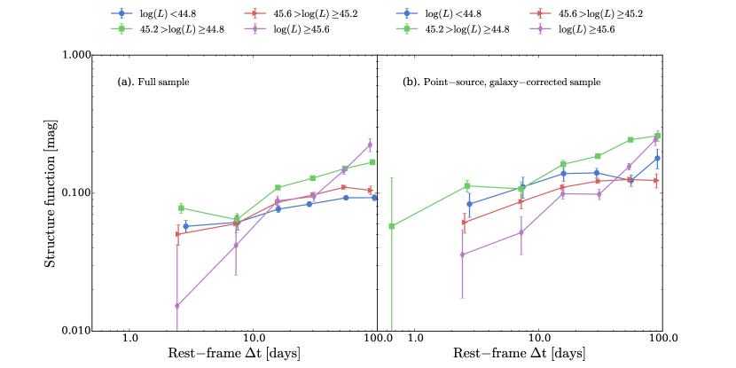
Figure 13.— Left panel: The structure functions of the $5100\ \rm{\AA}$ continuum for the SDSS-RM sample. The structure functions roughly increase with $\Delta t$ but are not monotonic functions of $L_{\rm{Bol}}$. This is likely due to the contamination by galaxy emission and the effects of variable seeing for extended sources. Right panel: The structure functions of the $5100\ \rm{\AA}$ continuum for the SDSS-RM point-source sample, with galaxy emission subtracted using the spectral decomposition of Shen et al. (2015b) (and removing sources with $>50\%$ host contribution). After the host-galaxy effects are removed, sources in low-luminosity bins show higher variability.

7. Structure Functions of Emission lines

In Section 6, we found that the variability of the continuum emission (at $3000\ \rm{\AA}$) is consistent with the DRW model. In this section, we present the structure functions of broad Mg ii and $\rm{H}\beta$. The study of the variability of broad emission lines provides information about the transfer function governing the response of the broad line region to incident continuum emission. The transfer function, in turn, reflects the structure and ionization state of the BLR.

7.1. Mg ii

We first consider the variability of Mg ii for SDSS-RM sources. We again divided our sources into the same four $L_{\rm{Bol}}$ bins as we did for the $3000\ \rm{\AA}$ continuum and calculated the structure function for each bin. We binned quasars by the continuum luminosity rather than the line luminosity so that it is easier to compare to the structure function of continuum emission. Our results are presented in the left panel of Figure 14.

Compared to the $3000\ \rm{\AA}$ continuum, the structure functions of Mg ii also increase with $\Delta t$ and (weakly) decrease with $L_{\rm{Bol}}$. We argue that this similarity is consistent with the idea that the variability of Mg ii is driven by the variability of the continuum emission (see the cross correlation analysis of Shen et al., 2015c).

The structure functions of Mg ii also differ from those of the $3000\ \rm{\AA}$ continuum in several aspects. First, the variability amplitude of the $3000\ \rm{\AA}$ continuum is generally larger than that of Mg ii, for each luminosity bin. In addition, the difference between the variability amplitudes of the $3000\ \rm{\AA}$ continuum and those of Mg ii decrease with $L_{\rm Bol}$ (similar to the results of Section 3). We also found the shapes of the structure functions of Mg ii and those of the $3000\ \rm{\AA}$ continuum are different by performing the same statistical hypothesis test we did in Section 6.1. We found that, for all four luminosity bins, the null hypothesis is rejected (i.e., the $p$ value of the chi-squared test is $\ll 0.01$). That is, our data indicate different slopes for the Mg ii and the $3000\ \rm{\AA}$ continuum structure functions. Note that Mg ii typically has larger measurement errors, and we expect it suffers from a stronger bias than the $3000\ \rm{\AA}$ continuum. To ensure the observed differences in shapes are not caused by the additional bias, we performed the “DRW simulation” described in Section 6.1 for Mg ii. We found that this simulation cannot reproduce the observed structure functions of Mg ii (both the normalization factors and shapes). Therefore, we conclude that the differences between the slopes for the Mg ii and the $3000\ \rm{\AA}$ continuum structure functions are intrinsic.

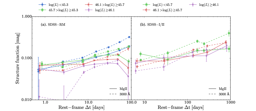
Figure 14.— Left panel: The structure functions of Mg ii (solid lines) for SDSS-RM sources. For comparison, we also present the structure functions of the $3000\ \rm{\AA}$ continuum (only using sources with well-measured Mg ii). It is evident that the structure functions of Mg ii depend on $L_{\rm Bol}$ in the same way as the $3000\ \rm{\AA}$ continuum. This result is consistent with the idea that the variability of Mg ii is driven by continuum variability. However, the $3000\ \rm{\AA}$ continuum is more variable than Mg ii. Also, the slopes of the Mg ii and $3000\ \rm{\AA}$ continuum structure functions are different (the structure function of Mg ii is shallower in each luminosity bin). Note that the apparent variability decrease at $\Delta t\sim 100$ days is likely due to the fact that the spectrophotometric errors dominate over the intrinsic variability. Right panel: The structure functions of Mg ii (solid lines) for SDSS-I/II sources. For comparison, we also present the structure functions of the $3000\ \rm{\AA}$ continuum (only using sources with well-measured Mg ii). Considering the fact that SDSS-I/II sources are generally more luminous than SDSS-RM sources, we only created three luminosity bins.

The right panel of Figure 14 shows the Mg ii structure functions for the SDSS-I/II quasars. The variability amplitude of Mg ii is again smaller than that of the $3000\ \rm{\AA}$ continuum for each luminosity bin. We also compared the shapes of the structure functions of Mg ii and those of the $3000\ \rm{\AA}$ continuum by performing the same hypothesis test. We found that, for the two low-luminosity bins, the shapes of the structure functions of Mg ii and those of the $3000\ \rm{\AA}$ continuum are different (i.e., the $p$ value is $\ll 0.01$). For the highest luminosity bin (i.e., the $\log L_{\rm{Bol}}>46.1$ bin), the $p$ value under the null hypothesis is $0.012$, and we cannot reject the idea that the shapes are the same. If we restrict the comparison to rest-frame timescales $\Delta t>100\ \rm{days}$ (the timescales that are not covered by the SDSS-RM data), we found that we cannot reject the null hypothesis and the Mg ii and the $3000\ \rm{\AA}$ continuum structure functions have consistent shapes in all luminosity bins (the $p$ value under the null hypothesis is $\gg 0.01$). The statistical test at $\Delta t>100$ days is limited, however, by having only three data points in each luminosity bin and therefore lacks power to reject the null hypothesis (the difference in slope $\beta$ is poorly constrained to be $\lesssim 0.5$).

7.2. $\rm{H}\beta$

In this section, we study the structure functions of $\rm{H}\beta$ for the SDSS-RM and SDSS-I/II data. In order to compare the structure functions of $\rm{H}\beta$ to that of the $3000\ \rm{\AA}$ continuum, we only consider sources with “well-measured” (i.e., satisfying our selection criteria) $\rm{H}\beta$ and $3000\ \rm{\AA}$ continuum. We choose the $3000\ \rm{\AA}$ continuum instead of the $5100\ \rm{\AA}$ continuum because the latter is significantly affected by galaxy emission (see Section 6.2). Due to the limited total number of sources, we do not divide our sources by luminosity. Figure 15 shows our results.

It is evident that, for both SDSS-RM and SDSS-I/II sources, the variability of $\rm{H}\beta$ is smaller than that of the $3000\ \rm{\AA}$ continuum on timescales of rest-frame $\Delta t>20\ \rm{days}$. We compared the shape of the structure function of $\rm{H}\beta$ with that of the $3000\ \rm{\AA}$ continuum by performing the same hypothesis test we did for Mg ii. From this test, the shapes of the $\rm{H}\beta$ and continuum structure functions are significantly different (i.e., the $p$ value under the null hypothesis is $\ll 0.01$). However, if we again restrict the comparison to rest-frame $\Delta t>100\ \rm{days}$, the hypothesis that the shapes of the structure functions of $\rm{H}\beta$ and the $3000\ \rm{\AA}$ continuum are the same cannot be rejected (the $p$ value under the null hypothesis is $\gg 0.01$). Again, the statistical test at $\Delta t>100$ days is limited (the “allowed” difference in slope $\beta$ is only constrained to be $\lesssim 0.8$).

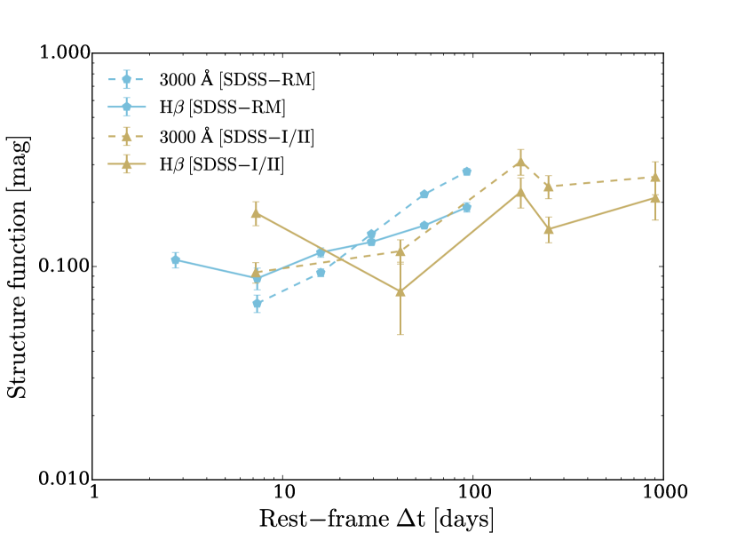
Figure 15.— The structure functions of $\rm{H}\beta$ for SDSS-RM sources (pentagons) and SDSS-I/II sources (triangles). As a comparison, we also included the structure functions of the $3000\ \rm{\AA}$ continuum (dashed lines). $\rm{H}\beta$ is less variable than the $3000\ \rm{\AA}$ continuum. The shapes of the structure functions of $\rm{H}\beta$ and the $3000\ \rm{\AA}$ continuum are different on timescales $\Delta t<100\ \rm{days}$. On longer timescales, the shapes are similar. Note that only quasars with “well-measured” $\rm{H}\beta$ and $3000\ \rm{\AA}$ continuum are included.

We also compare the structure function of Mg ii with that of $\rm{H}\beta$. Only $26$ sources with “well-measured” Mg ii and $\rm{H}\beta$ are included. Due to the limited sample size, we do not bin by luminosity. Our results are presented in Figure 16. For the SDSS-RM sample, the variability amplitude of $\rm{H}\beta$ is larger than that of Mg ii, which was also indicated by the analysis described in Section 3.2 (Figure 9). For the SDSS-I/II sample, the difference is not significant.

We again performed the same hypothesis test to test whether the structure function of Mg ii and that of $\rm{H}\beta$ share the same shape. For the SDSS-RM sample, our test indicates that the Mg ii and $\rm{H}\beta$ structure functions have statistically different shapes (i.e., the $p$ value under the null hypothesis is $<0.01$). For the SDSS-I/II sample, the null hypothesis cannot be rejected by our data (i.e., the $p$ value under the null hypothesis is $\gg 0.01$, and the difference in slope $\beta$ is $\lesssim 0.3$).

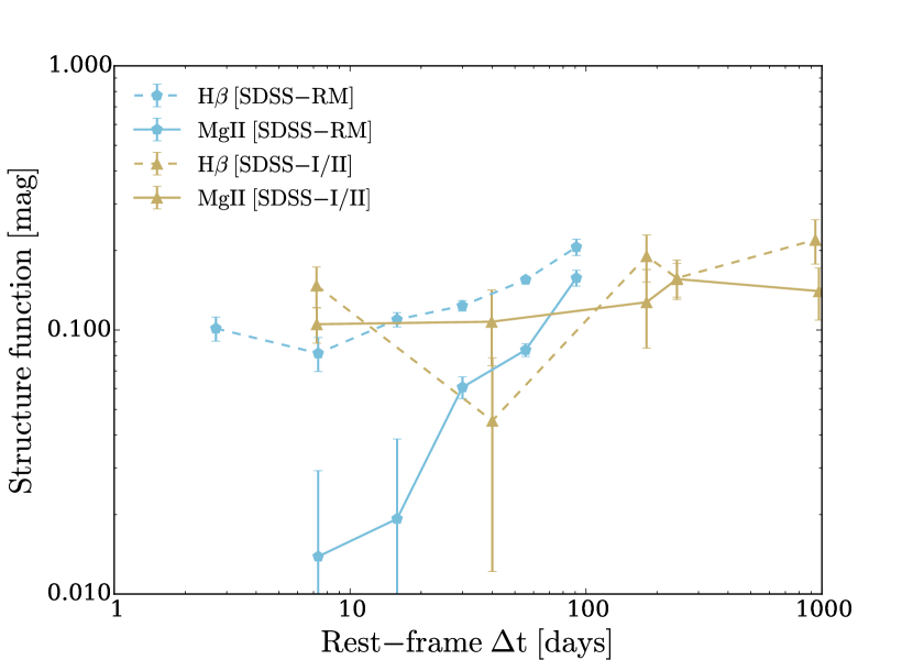
Figure 16.— A comparison of the structure functions of Mg ii with those of $\rm{H}\beta$ for both SDSS-RM (pentagons) and SDSS-I/II (triangles) sources. For the SDSS-RM sources, the shapes of the structure functions of Mg ii and those of $\rm{H}\beta$ are different. For the SDSS-I/II sources, our statistical hypothesis test indicates that the shapes of the structure functions of Mg ii and those of $\rm{H}\beta$ are not significantly different. Note that only quasars with “well-measured” Mg ii and $\rm{H}\beta$ are included.

8. Discussion: The Nature of Quasar Variability

8.1. Quasar variability and quasar properties

As revealed by many previous investigations (e.g., Kelly et al., 2009; MacLeod et al., 2012), quasar variability is controlled by quasar properties (see Eq. 8). In Figure 12, we showed that the M10 relations can effectively reproduce our results. Therefore, our results are consistent with the idea that quasar properties (e.g., $L_{\rm Bol}$ and $M_{\rm BH}$) determine the structure of the accretion disk which in turn controls the instabilities in the accretion disk.

The thermal timescale of the accretion disk is (e.g., Kato et al., 1998; Kelly et al., 2009)

$$t_{\rm{TH}}\approx 53.1\times(\frac{\alpha}{0.01})^{-1}(\frac{M_{\rm{BH}}}{10^{8}\ M_{\odot}})(\frac{R}{10\ R_{\rm{S}}})^{3/2}\ \rm{days}\\ ,$$ (9)

where $\alpha$ is the dimensionless viscosity parameter (Shakura & Sunyaev, 1973), and $R_{\rm{S}}=2GM_{\mathrm{BH}}/c^{2}$ is the Schwarzschild radius. Assuming the $3000\ \rm{\AA}$ continuum is produced at $\sim 30\ R_{\rm{S}}$ (based on microlensing observations, see Eq. 4 of Morgan et al., 2010), the expected thermal timescale is around $174\ \rm{days}$ (for $\alpha=0.05$ and $M_{\mathrm{BH}}=10^{8.5}\ M_{\odot}$ which is the median value for our sample). The estimated $\tau$ ($\sim 199.5^{+116.7}_{-73.6}$ days, see Section 6.1) from the SDSS-I/II data is consistent with the thermal timescale of the accretion disk. Therefore, the DRW model can be explained by thermal fluctuations in the accretion disk (see also Kelly et al., 2009). On timescales much smaller than $\tau$, the thermal fluctuations (which are ultimately driven by magnetic turbulence, see recent numerical simulations, e.g., Hirose et al., 2009; Jiang et al., 2013, and also a detailed theoretical calculation by Lin et al. 2012) in the accretion disk drive the random-walk-like fluctuations in $L$. On longer timescales ($\gg\tau$), the disk can adjust itself to the thermal fluctuations and therefore the fluctuations in $L$ are purely white noise and/or are related to fluctuations in $\dot{M}$ (which correspond to the much longer viscous timescale, see e.g., Lyubarskii, 1997; Kelly et al., 2011).

It has been found that, on short timescales ($\sim$ days), the variability of quasar continuum emission is smaller than the DRW model predicts (e.g., Mushotzky et al., 2011; Zu et al., 2013; Kasliwal et al., 2015). Although SDSS-RM includes some variability data on these short timescales, the median spectroscopic sampling interval over the campaign was $\sim 4$ days in observed frame (i.e., $\gtrsim 1.3$ days in rest frame), and the large measurement and spectrophotometric errors make it difficult to place meaningful constraints on variability over $\Delta t\lesssim 5$ days. In particular, on very short timescales (where the intrinsic variability is small), the observed variability is dominated by the measurement and spectrophotometric errors rather than the intrinsic variability, and the structure function estimation suffers from significant bias (as illustrated in the middle panel of Figure 12).

8.2. Implications for Reverberation-Mapping Projects

In the SDSS-RM overview paper, Shen et al. (2015a) simulated the expected results from the SDSS-RM project. In this section, we explore the validity of these simulations and the implications of our results for future reverberation-mapping campaigns.

We start with the model used to generate quasar continuum light curves. In Shen et al. (2015a), they generated continuum light curves based on the DRW model and the M10 relations. As shown in Section 6.1, the DRW model indeed describes the rest-frame $10-100\ \rm{day}$ variability of quasar continuum emission well. The M10 relations can also effectively reproduce the structure function, although low-luminosity quasars may actually be slightly more variable (by a factor of $\sim 1.3$) than predicted by extrapolating the M10 relations. Therefore, the initial SDSS-RM simulations of quasar continuum light curves are likely to be valid.

Justifying the transfer function is difficult since we actually cannot constrain its exact shape. However, assuming the width of the transfer function to be $10\%$ of the time lag (i.e., not a $\delta$ function) is consistent with our results. We find that the transfer function is likely to have a width in the range of $1-100$ days (see Section 8.3). Our loose constraints on the transfer-function width are consistent with width estimates from velocity-resolved reverberation mapping results (e.g., Grier et al., 2013; De Rosa et al., 2015).

Last but not least, we find that, for a large population of quasars, Mg ii varies significantly. Like $\rm{H}\beta$, Mg ii is likely to respond to the continuum emission (as they depend on quasar luminosity in a similar way) and therefore has the potential to be used for reverberation-mapping campaigns.

8.3. The Broad Emission Line Transfer Function

The detailed ionization state, dynamical structure, and kinematic motions of the BLR are still poorly constrained from observations. In Sections 3 and 7, we compared the variability of two broad emission lines (Mg ii and $\rm{H}\beta$) with that of $L_{3000}$. We demonstrated that both broad lines were less variable than the continuum emission (at fixed time separation and luminosity). In addition, the structure functions of the broad emission lines are shallower than the $3000\ \rm{\AA}$ continuum structure functions, indicating that the broad emission lines are not driven by the same DRW model which describes the variability of the $3000\ \rm{\AA}$ continuum. $\rm{H}\beta$ is typically more variable than Mg ii. In this section, we discuss the implications of these results for our understanding of BLR.

Let us first define a transfer function $\Phi(t_{s})$ which governs the response of the emission-line light curve $f_{l}(t)$ to the incident continuum emission $f_{c}(t)$, after a light-travel time delay $t_{s}$ (e.g., Blandford & McKee, 1982):

$$f_{l}(t)=\int dt_{s}\Phi(t_{s})f_{c}(t-t_{s})$$ (10)

where $f_{c}(t)$ is the light curve of the continuum emission. The broad-line structure functions are flatter than those of the continuum (i.e., $3000\ \rm{\AA}$, whose variability is consistent with the DRW model). If the variability of the EUV continuum is similar to the variability of the $3000\ \rm{\AA}$ continuum, our results demonstrate that the transfer functions of the broad emission lines are not consistent with the $\delta$-function: a broad (in time) transfer function would effectively flatten the input structure function. Mg ii and $\rm{H}\beta$ are driven by ionizing photons of $E>15\ \rm{eV}$ and $E>13.6\ \rm{eV}$, respectively. This higher-energy flux likely has a shorter $\tau$ than than the $3000\ \rm{\AA}$ continuum, leading to an apparently flatter structure function. However, extrapolating the M10 relations to $E\sim 15\ \rm{eV}$, the expected $\tau$ is still $\sim 100\ \rm{days}$.

The shape differences disappear when we only consider variability on timescales of rest-frame $\Delta t>100\ \rm{days}$. This conclusion, if it is robust, suggests that the width of the transfer function for Mg ii is (for our SDSS-RM sample) less than $100\ \rm{days}$. The same conclusion holds for $\rm{H}\beta$. Therefore, on longer timescales, the variability of Mg ii (or $\rm{H}\beta$) has similar timescale-dependence to the variability of the $3000\ \rm{\AA}$ continuum.

Our data demonstrate that both Mg ii and $\rm{H}\beta$ have lower variability amplitude than the $3000\ \rm{\AA}$ continuum. This result is also consistent with MacLeod et al. (2012) (see their Figure $13$) who (indirectly) find that Mg ii is less variable than the local continuum by exploring the photometric variability as a function of rest-frame wavelength (see also Ivezic et al., 2004). The EUV continuum which actually drives both lines is probably more variable than the $3000\ \rm{\AA}$ continuum, since variability increases with decreasing wavelength (e.g., Vanden Berk et al., 2004; MacLeod et al., 2010). Indeed, early EUV observations reveal strong variability (a factor of $2$) even within $1\ \rm{day}$ (e.g., Marshall et al., 1997; Uttley et al., 2000; Halpern et al., 2003). Thus the amplitude of the transfer function is likely to be significantly less than one, with the broad lines less variable than their incident continuum. This result is consistent with detailed photoionization calculations (e.g., Korista & Goad, 2000, 2004).

Our data suggest that the difference between the $3000\ \rm{\AA}$ continuum and Mg ii variability decreases with $L_{\rm Bol}$. That is, as quasar luminosity decreases, the variability amplitude of Mg ii increases more slowly than $3000\ \rm{\AA}$. This may be related to a changing ionization structure as luminosity changes: this effectively changes the radius of the BLR (as inferred by reverberation-mapping studies, which measure a responsivity-weighted radius), and the responsivity (defined as the ratio of the variability of emission lines to that of continuum emission) increases with increasing radius (Korista & Goad, 2004).

We find that $\rm{H}\beta$ is slightly more variable than Mg ii, in agreement with previous quasar spectral variability studies (Kokubo et al., 2014). The ionizing continuum that drives $\rm{H}\beta$ ($E>13.6\ \rm{eV}$) is similar to that driving Mg ii ($E>15\ \rm{eV}$). Therefore, the differences between Mg ii and $\rm{H}\beta$ variability are not likely to be due to the differences in ionizing continuum.

The variability differences might be caused by the fact that $\rm{H}\beta$ is a recombination line while Mg ii is a collisionally excited resonance line (e.g., MacAlpine, 1972; Netzer, 1980). Each of these processes depends on the changes in incident EUV flux in a different way. This difference might lead to a lower variability of Mg ii than $\rm{H}\beta$.

The differences between Mg ii and $\rm{H}\beta$ might also be caused by the different optical depth for the two emission lines. Since Mg ii is a resonance line, its optical depth is expected to be larger than that of $\rm{H}\beta$. At a sufficiently high density, Mg ii photons will be absorbed and re-emitted many times before escaping the BLR. This process might effectively stabilize changes in Mg ii luminosity by diluting the response to continuum changes.

The difference between Mg ii and $\rm{H}\beta$ could also indicate the structure of the BLR that emits Mg ii is different from the BLR that produces $\rm{H}\beta$. For instance, it is possible the BLR material that emits Mg ii extends to larger radius that that of $\rm{H}\beta$. Therefore, as the quasar continuum varies, Mg ii responds on a wider range of timescales, and the variability of Mg ii is again diluted.

Some of these ideas are included in the “local optimally-emitting cloud” (LOC) model which assumes that the BLR consists of various density gas clouds. A detailed photoionization equilibrium calculation of the LOC model reveals that Mg ii is less variable than $\rm{H}\beta$ over most of the typical range of BLR conditions (Korista et al., 1997; Korista & Goad, 2000, 2004).

Our data also indicate that the shapes of the structure functions of Mg ii and $\rm{H}\beta$ are different at $\Delta t<100$ days. These results suggest that the transfer functions of Mg ii and $\rm{H}\beta$ are also different in width: that is, the transfer functions of Mg ii and $\rm{H}\beta$ have different radial profiles. At longer timescales ($\Delta t>100$ days), the shapes of the structure functions of Mg ii and $\rm{H}\beta$ are similar (the difference in slope $\beta$ is $\lesssim 0.3$). This result is expected since the widths of the transfer functions for Mg ii and $\rm{H}\beta$ are both likely less than $100$ days.

Our comparison of $\rm{H}\beta$ and Mg ii variability is largely limited to low-luminosity quasars due to the low-redshift requirement for each spectrum to include both lines. It is possible that the relative difference in responsivity between $\rm{H}\beta$ and Mg ii has a luminosity dependence (Korista et al., 1997; Korista & Goad, 2000, 2004), and comparing the different variability behavior of $\rm{H}\beta$ and Mg ii over a larger luminosity range would place additional constraints on the physical conditions and excitation sources of the BLR.

9. Summary

Using SDSS-RM and SDSS I/II data, we studied the variability of continuum emission probed at $3000\ \rm{\AA}$ and $5100\ \rm{\AA}$ continuum and the variability of the Mg ii and $\rm{H}\beta$ broad emission lines. Our results can be summarized as follows:

1. We determined the variability of Mg ii for a large quasar sample. We found that, like $\rm{H}\beta$, Mg ii varies, consistent with the scenario that Mg ii varies in response to the variability of the continuum emission (Figures 5 and 14; Sections 3 and 7).

2. We found that the shapes of the structure functions of the $3000\ \rm{\AA}$ continuum and those of broad emission lines are different, indicating the transfer functions governing the response of broad emission lines are broad in time. We also found that the difference between the variability of the $3000\ \rm{\AA}$ continuum and broad emission lines decreases with quasar luminosity (Figures 6 and 14; Sections 3 and 7), consistent with photoionization model predictions of Korista & Goad (2004).

3. We confirmed that the continuum variability on timescales of $\Delta t>5$ days is well-described by the DRW model (the difference in slope $\beta\lesssim 0.1$, see Figure 12 and Section 6.1), and that the continuum variability is a function of quasar properties (Figure 12. Section 8.1).

4. Emission from the host galaxy introduces a significant bias to the measured quasar variability at rest-frame $5100\ \rm{\AA}$ (Figure 13; Section 6.2).

5. We also found that the structure functions of Mg ii and $\rm{H}\beta$ have statistically different shapes (Figure 16; Sections 7.2 and 8.3). Also, $\rm{H}\beta$ is slightly more variable than Mg ii, consistent with the predictions of the LOC model (e.g., Korista & Goad, 2000, 2004). Our results may be explained by the fact that the two broad emission lines have different radiative mechanisms, geometrical configurations, and/or optical depths (see Sections 3 and 8.3).

Our results indicate that the predictions of the SDSS-RM project are accurate (see Section 8.2). Continuing observations should enable accurate estimation of $M_{\rm BH}$ for a large set of $z>1$ quasars utilizing the reverberation-mapping technique (using both $\rm{H}\beta$ and Mg ii, see Shen et al., 2015c).

Appendix A STRUCTURE FUNCTION ESTIMATORS

The structure function measures the statistical dispersion of two observations separated by $\Delta t$. Several popular non-parametric statistical dispersion estimators have been proposed: the interquartile range (IQR), the median absolute deviation (MAD), the average absolute deviation (AAD), and the standard deviation. Their definitions are:

• the IQR estimator (used by MacLeod et al., 2012): see Section 5.1;

• the MAD estimator:

  $$\mathrm{SF_{MAD}}(\Delta t)=\sqrt{(1.48\mathrm{MAD}(\Delta m))^{2}-\widetilde{\sigma^{2}_{\rm{e}}}}\\ ,$$

  where $\mathrm{MAD}(\Delta m)=\widetilde{\left|\Delta m-\widetilde{\Delta m}\right|}$;

• the AAD estimator (used by Vanden Berk et al., 2004):

  $$\mathrm{SF_{AAD}}(\Delta t)=\sqrt{\frac{\pi}{2}\left<\left|\Delta m\right|\right>^{2}-\left<\sigma^{2}_{\rm{e}}\right>}\\ .$$

• the maximum-likelihood standard deviation (ML) estimator: the standard deviation can be measured using the maximum-likelihood method proposed by Almaini et al. (2000) (see their Section 3.1).

We subtract the spectrophotometric error from each structure function calculated from the stars using the same estimator. The constant factors in each of the four structure-function estimators normalizes them to be equivalent to the standard deviation of a Gaussian distribution (assuming Gaussian measurement and spectrophotometric errors). Our data and uncertainties have non-Gaussian tails, which lead to differences in the estimators: for distributions with larger tails than a Gaussian, the IQR and MAD estimators are smaller than the AAD and standard deviation estimators.

The four structure functions of the $3000\ \rm{\AA}$ continuum are plotted in Figure 17. Note that if the number of flux pairs for a given $\Delta t$ bin is less than $10$, we do not calculate the variability in this particular bin. For each $L_{\rm{Bol}}$ bin with many quasars, each quasar has different intrinsic variability and measurement/spectrophotometric errors. That is, the ensemble distribution of $\Delta m$ is a superposition of many Gaussian distributions and is not a perfect Gaussian but instead has exponential tails. Moreover, the subtraction of measurement and spectrophotometric errors (i.e., subtract $\tilde{\sigma_{e}}$ or $\left<\sigma_{e}\right>$) has an effect on the estimation of the ensemble structure function. This results in slightly different results for each of the four structure-function estimators.

For the AAD estimator, since we are subtracting the mean value of measurement and spectrophotometric errors, our results may be biased by quasars with measurement and spectrophotometric errors that are much larger than the intrinsic variability. The standard deviation estimator uses individual errors (using the maximum likelihood method), and so is stable against quasars with relatively large measurement and spectrophotometric errors. The IQR and MAD estimators use median values of the measurement and spectrophotometric errors, and so are also stable against quasars with large measurement and spectrophotometric errors. Moreover, the IQR and MAD estimators are also robust against outliers in the distribution of $\Delta m$.

The IQR, MAD and ML (or standard deviation) estimators give similar results: (1) the ensemble structure function increases with $\Delta t$ in a similar way; (2) the ensemble structure function decreases with quasar luminosity in a similar way.

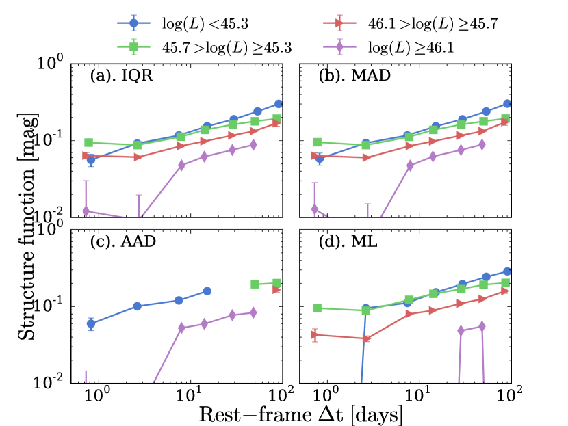
Figure 17.— The structure function of the $3000\ \rm{\AA}$ continuum for each quasar luminosity bin. The IQR, MAD, AAD, and ML estimators are shown. The IQR and MAD estimators are stable against measurements with relatively large uncertainties and also robust against outliers.

The four structure functions of the $5100\ \rm{\AA}$ continuum are plotted in Figure 18 for the full “clean” sample of SDSS-RM quasars. Figure 19 shows only point sources with galaxy emission subtracted, using the spectral decomposition of Shen et al. (2015b) and removing quasars with $>50\%$ host contribution at $5100\ \rm{\AA}$.

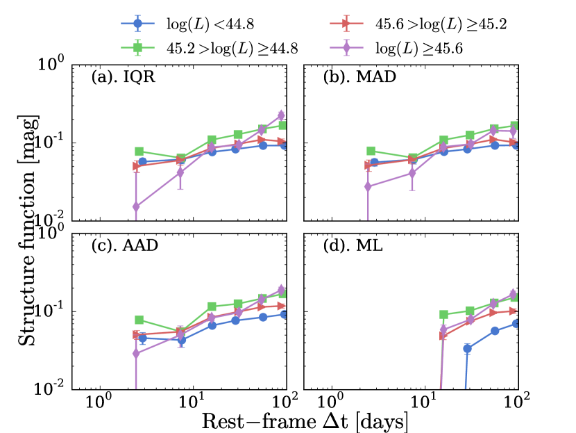
Figure 18.— The structure function of the $5100\ \rm{\AA}$ continuum for each luminosity bin. The IQR, MAD, AAD, and ML estimators are shown.

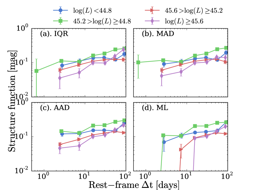
Figure 19.— The structure function of the $5100\ \rm{\AA}$ continuum for each luminosity bin. The IQR, MAD, AAD, and ML estimators are shown. Only point sources are included, and galaxy emission is subtracted.

The four structure functions of Mg ii and $\rm{H}\beta$ are shown in Figures 20 and 21, respectively. In all four cases, the broad-line structure functions are flatter than the continuum structure functions.

As shown in this section, the IQR and MAD estimators are robust against outliers. We prefer the IQR since it has been adopted in MacLeod et al. (2012).

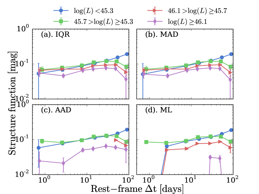
Figure 20.— The structure function of Mg ii for each luminosity bin. The IQR, MAD, AAD, and ML estimators are shown.

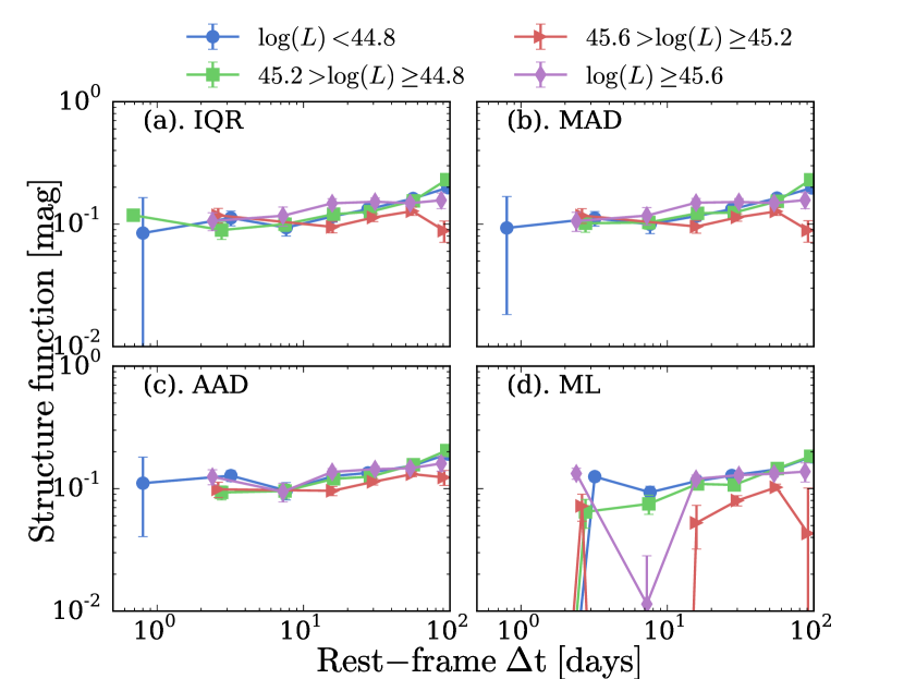
Figure 21.— The structure function of $\rm{H}\beta$ for each luminosity bin. The IQR, MAD, AAD, and ML estimators are shown.

Appendix B SDSS-RM SPECTROPHOTOMETRIC UNCERTAINTY

In this section, we quantify the spectrophotometric errors in the SDSS-RM survey. The spectra were calibrated using $70$ standard stars. Therefore, the variability of standard stars used in the SDSS-RM survey should reflect the spectrophotometric errors. Note that one star was found to be intrinsically variable, and five other stars have an epoch with a “dropped” spectrum. We do not remove these stars when accounting for the variability of standard stars since these stars were not removed when calibrating the spectra. Due to their small number, these stars do not significantly affect the flux calibration.

B.1. STRUCTURE FUNCTION OF STANDARD STARS

As a first step, we present the observed distribution of $\Delta m$ for standard stars. To do so, we created $21$ wavelength bins starting from $3700\ \rm{\AA}$, each with a width of $300\ \rm{\AA}$. We then calculated the average flux in each bin at every epoch for every standard star. As a final step, we again calculated $\Delta m$ for any two observations separated by $\Delta t$.

In Figure 22, we plot the distribution of $\Delta m$ for standard stars. It is evident that the variability of standard stars depends strongly on wavelength. The variability at $\sim 7000\ \rm{\AA}$ is the smallest ($\sim 0.06\ \rm{mag}$). Also, the variability increases significantly to both the short-wavelength ($\sim 0.1\ \rm{mag}$) and the long-wavelength ends ($\sim 0.07\ \rm{mag}$). This is due to the fact that the flux calibration is done using $r$-band only. Note that the distributions are not Gaussian but are instead Laplacian which indicates that the spectrophotometric errors are not perfectly Gaussian (and the tails are not due to the variable stars).

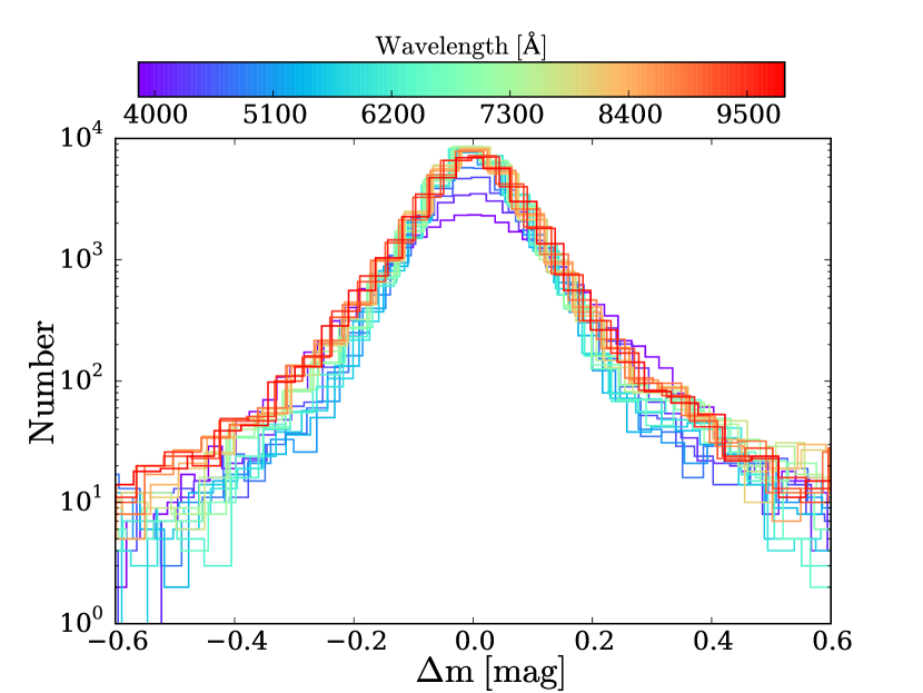
Figure 22.— The distributions of $\Delta m$ for standard stars. Again, $\Delta m=-2.5\log(f_{2}/f_{1})$. There are exponential tails in the distribution of $\Delta m$ for standard stars. The variability is the smallest at $\sim 6000-7000\ \rm{\AA}$ (since the flux calibration is done using the $r$-band), and higher at both small and large wavelengths.

Since the quasar spectra were calibrated using standard stars, we can then use the structure function of standard stars as an estimation of spectrophotometric errors. Note that the structure function quantifies the variability of a flux pair, and therefore the spectrophotometric uncertainty for a single epoch is the structure function divided by $\sqrt{2}$. The variability of standard stars depends on wavelength, and so we calculated the structure function of standard stars in each wavelength bin separately. Figure 23 plots our results. It is evident that the structure function of the standard stars is largely constant with $\Delta t$ for each wavelength bin. There is a small increase (within $0.02\ \rm{mag}$) at $\Delta t>20\ \rm{days}$: this is associated with the time between different dark runs in the SDSS-RM observations. The structure function of standard stars depends on wavelength and is the smallest in the $\sim 6000-7000\ \rm{\AA}$ band. In the $\sim 6000-7000\ \rm{\AA}$ band, the scale of the variability is only $\sim 0.06\ \rm{mag}$ (for the IQR estimator). Therefore, for a single epoch, the spectrophotometric error of our SDSS-RM data is expected to be not smaller than $\sim 0.06/\sqrt{2}\approx 0.04\ \rm{mag}$ (also see Figure 20 of Shen et al., 2015a).

The spectrophotometric error of the SDSS-I/II data for a single epoch is assumed to be $0.04\ \rm{mag}$ (Adelman-McCarthy et al., 2008).

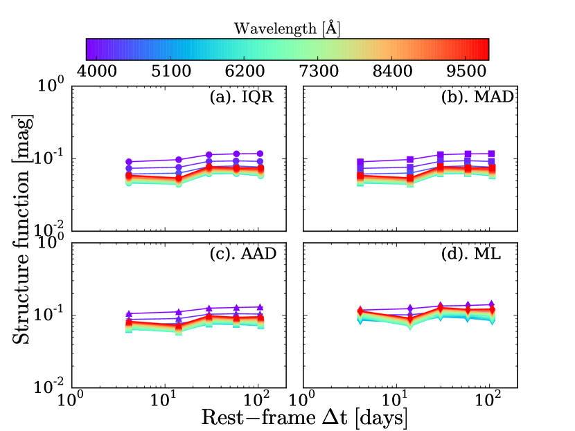
Figure 23.— The structure function of standard stars for each wavelength bin. The spectrophotometric uncertainty of a single epoch is the structure function divided by $\sqrt{2}$. The spectrophotometric errors depend on wavelength and have a minimum value at $6000-7000\ \rm{\AA}$ (of $\sim 0.06/\sqrt{2}\ \rm{mag}$). Furthermore, the structure function only slightly depends on $\Delta t$ (increasing by $0.02\ \rm{mag}$ at $\Delta t\gtrsim 20$ days).

B.2. [O iii]

We also checked the variability of [O iii]$\lambda 5007$ (hereafter [O iii]). Physically, we expect that there is no intrinsic variability of [O iii]  on timescales of $\sim 100\ \rm{days}$. That is, the variability of [O iii] should be equivalent to that of standard stars. To verify this, we calculated the structure function of [O iii]  while subtracting only measurement errors (i.e., $\sigma_{\rm{e}}$ in Section 5.1 only accounts for measurement errors) and compared the structure functions with the expected spectrophotometric errors of the flux pairs. The expected spectrophotometric errors are the average of the structure function of standard stars at the same wavelength as the [O iii]  (i.e., $5007(1+z)\ \rm{\AA}$, where $z$ is the redshift of the quasar). We divided our sources into subsamples of point sources and extended sources in order to investigate the additional variability due to variable seeing. To investigate the effects of measurement errors on the estimation of the structure function, we binned quasars by $\widetilde{\rm{S/N}}$. For each sub-sample, we created three bins: $15\leq\widetilde{\rm{S/N}}<25$, $25\leq\widetilde{\rm{S/N}}<35$, $\widetilde{\rm{S/N}}\geq 35$. We required a minimum of $\widetilde{\rm{S/N}}>15$ so that the measurement errors do not dominate over the spectrophotometric errors. We then calculated the structure function of each bin.

Figure 24 shows the structure function for the sub-sample of point sources. The variability of [OIII] for point sources is nearly identical to the expected spectrophotometric errors. For each bin, we calculated the difference between the structure function and the spectrophotometric errors in quadrature. The difference is no more than $0.03$ mag, and there is no systematic offset. In addition, the variability is not a monotonic function of $\widetilde{\rm{S/N}}$ which suggests our $\widetilde{\rm{S/N}}>15$ cut reliably prevents a bias from large measurement errors dominating the observed variability. Therefore, we conclude that our estimation of the spectrophotometric errors is robust.

Figure 25 plots the structure function for the sub-sample of extended sources. It is evident that, for each bin, [O iii]  shows excess variability compared to the spectrophotometric errors. This is due to additional variability ($\sim 0.07-0.1\ \rm{mag}$ in the IQR) from variable seeing in addition to the spectrophotometric errors. Additional variability from seeing changes has consequences for the structure-function estimates of extended sources (e.g., if there is a substantial host-galaxy component to the measured $5100\ \rm{\AA}$ luminosity, see Section 6.2).

Figure 24.— The structure functions of [O iii] for point sources. Note that the structure functions presented here were only corrected for measurement errors. The dashed lines represent the expected spectrophotometric errors which are obtained according to the redshift distribution of quasars in each bin. It is evident that, for point sources, [O iii] does not show intrinsic variability. This result indicates that our estimation of the spectrophotometric errors is robust.

Figure 25.— The structure functions of [O iii] for extended sources only. Note that the structure functions that are presented here were only corrected for measurement errors. The dashed lines represent the expected spectrophotometric errors which are obtained according to the redshift distribution of quasars in each bin. Extended sources show variability beyond the spectrophotometric errors which is likely due to seeing effects (i.e., the variable seeing in different epochs).

References

- Adelman-McCarthy et al. (2008) Adelman-McCarthy, J. K., Agüeros, M. A., Allam, S. S., et al. 2008, ApJS, 175, 297
- Ai et al. (2010) Ai, Y. L., Yuan, W., Zhou, H. Y., et al. 2010, ApJ, 716, L31
- Almaini et al. (2000) Almaini, O., Lawrence, A., Shanks, T., et al. 2000, MNRAS, 315, 325
- Bauer et al. (2009) Bauer, A., Baltay, C., Coppi, P., Ellman, N., Jerke, J., Rabinowitz, D. & Scalzo, R. 2009, ApJ, 696, 1241
- Blandford & McKee (1982) Blandford, R. D. & McKee, C. F. 1982, ApJ, 255, 419
- Bolton et al. (2012) Bolton, A. S., Schlegel, D. J., Aubourg, É., et al. 2012, AJ, 144, 144
- Cackett et al. (2015) Cackett, E. M., Gultekin, K., Bentz, M. C., et al. 2015, arXiv:1503.02029
- Clavel et al. (1991) Clavel, J., Reichert, G. A., Alloin, D., et al. 1991, ApJ, 366, 64
- Czerny (2006) Czerny, B. 2006, Astronomical Society of the Pacific Conference Series, 360, 265
- Czerny et al. (1999) Czerny, B., Schwarzenberg-Czerny, A. & and Loska, Z. 1999, MNRAS, 303, 148
- Dawson et al. (2013) Dawson, K. S., Schlegel, D. J., Ahn, C. P., et al. 2013, AJ, 145, 10
- De Rosa et al. (2015) De Rosa, G., Peterson, B. M., Ely, J., et al. 2015, ApJ, 806, 128
- de Vries et al. (2005) de Vries, W. H., Becker, R. H., White, R. L. & Loomis, C. 2005, AJ, 129, 615
- Eisenstein et al. (2011) Eisenstein, D. J., Weinberg, D. H., Agol, E., et al. 2011, AJ, 142, 72
- Emmanoulopoulos et al. (2010) Emmanoulopoulos, D., McHardy, I. M., & Uttley, P. 2010, MNRAS, 404, 931
- Gaskell (2009) Gaskell, C. M. 2009, New Astron. Rev., 53, 140
- Giveon et al. (1999) Giveon, U., Maoz, D., Kaspi, S., Netzer, H. & Smith, P. S. 1999, MNRAS, 306, 637
- Grier et al. (2013) Grier, C. J., Peterson, B. M., Horne, K., et al. 2013, ApJ, 764, 47
- Gunn et al. (2006) Gunn, J. E., Siegmund, W. A., Mannery, E. J., et al. 2006, AJ, 131, 2332
- Halpern et al. (2003) Halpern, J. P., Leighly, K. M., & Marshall, H. L. 2003, ApJ, 585, 665
- Hawkins (2002) Hawkins, M. R. S. 2002, MNRAS, 329, 76
- Hirose et al. (2009) Hirose, S., Blaes, O., & Krolik, J. H. 2009, ApJ, 704, 781
- Hook et al. (1994) Hook, I. M., McMahon, R. G., Boyle, B. J. & Irwin, M. J. 1994, MNRAS, 268, 305
- Hryniewicz et al. (2014) Hryniewicz, K., Czerny, B., Pych, W., et al. 2014, A&A, 562, AA34
- Ivezic et al. (2004) Ivezic, Ž., Lupton, R. H., Juric, M., et al. 2004, in IAU Symp. 222, The Interplay Among Black Holes, Stars and ISM in Galactic Nuclei, ed. Th. Storchi Bergmann, L.C. Ho, & H. R. Schmitt (Cambridge: Cambridge Univ. Press), 525
- Jiang et al. (2013) Jiang, Y.-F., Stone, J. M., & Davis, S. W. 2013, ApJ, 778, 65
- Kasliwal et al. (2015) Kasliwal, V. P., Vogeley, M. S., & Richards, G. T. 2015, arXiv:1505.00360
- Kaspi et al. (2000) Kaspi, S., Smith, P. S., Netzer, H., et al. 2000, ApJ, 533, 631
- Kato et al. (1998) Kato, S., Fukue, J., & Mineshige, S. 1998, Black-hole Accretion Disks (Kyoto: Kyoto University Press)
- Kelly et al. (2009) Kelly, B. C., Bechtold, J. & Siemiginowska, A. 2009, ApJ, 698, 895
- Kelly et al. (2011) Kelly, B. C., Sobolewska, M., & Siemiginowska, A. 2011, ApJ, 730, 52
- Kokubo et al. (2014) Kokubo, M., Morokuma, T., Minezaki, T., Doi, M., Kawaguchi, T., Sameshima, H. & Koshida, S. 2014, ApJ, 783, 46
- Korista et al. (1997) Korista, K., Baldwin, J., Ferland, G., & Verner, D. 1997, ApJS, 108, 401
- Korista & Goad (2000) Korista, K. T., & Goad, M. R. 2000, ApJ, 536, 284
- Korista & Goad (2004) Korista, K. T., & Goad, M. R. 2004, ApJ, 606, 749
- Krawczyk et al. (2013) Krawczyk, C. M., Richards, G. T., Mehta, S. S., et al. 2013, ApJS, 206, 4
- Laor (1998) Laor, A. 1998, ApJ, 505, L83
- Li & Cao (2008) Li, S.-L., & Cao, X. 2008, MNRAS, 387, L41
- Lin et al. (2012) Lin, D.-B., Gu, W.-M., Liu, T., Sun, M.-Y., & Lu, J.-F. 2012, ApJ, 761, 29
- Lusso et al. (2012) Lusso, E., Comastri, A., Simmons, B. D., et al. 2012, MNRAS, 425, 623
- Lyubarskii (1997) Lyubarskii, Y. E. 1997, MNRAS, 292, 679
- MacAlpine (1972) MacAlpine, G. M. 1972, ApJ, 175, 11
- MacLeod et al. (2008) MacLeod, C. L., Ivezić, Ž., de Vries, W., Sesar, B. & Becker, A. 2008, AIPC, 1082, 282
- MacLeod et al. (2010) MacLeod, C. L., Ivezić, Ž., Kochanek, C. S. et al. 2010, ApJ, 721, 1014 (M10)
- MacLeod et al. (2012) MacLeod, C. L., Ivezić, Ž., Sesar, B. et al. 2012, ApJ, 753, 106
- Margala et al. (2015) Margala, D., Kirkby, D., Dawson, K., et al. 2015, in preparation
- Marshall et al. (1997) Marshall, H. L., Carone, T. E., Peterson, B. M., et al. 1997, ApJ, 479, 222
- Morgan et al. (2010) Morgan, C. W., Kochanek, C. S., Morgan, N. D., & Falco, E. E. 2010, ApJ, 712, 1129
- Mushotzky et al. (2011) Mushotzky, R. F., Edelson, R., Baumgartner, W. & Gandhi, P. 2011, ApJ, 743, 12
- Netzer (1980) Netzer, H. 1980, ApJ, 236, 406
- Peterson (1993) Peterson, B. M. 1993, PASP, 105, 247
- Peterson (2014) Peterson, B. M. 2014, Space Sci. Rev., 183, 253
- Peterson et al. (1998) Peterson, B. M., Wanders, I., Bertram, R., et al. 1998, ApJ, 501, 82
- Peterson & Bentz (2006) Peterson, B. M. & Bentz, M. C. 2006, NewAR, 50, 796
- Reichert et al. (1994) Reichert, G. A., Rodriguez-Pascual, P. M., Alloin, D., et al. 1994, ApJ, 425, 582
- Richards et al. (2006) Richards, G. T., Lacy, M., Storrie-Lombardi, L. J., et al. 2006, ApJS, 166, 470
- Sesar et al. (2007) Sesar, B., Ivezić, Ž., Lupton, R. H., et al. 2007, AJ, 134, 2236
- Shakura & Sunyaev (1973) Shakura, N. I., & Sunyaev, R. A. 1973, A&A, 24, 337
- Shen (2013) Shen, Y. 2013, BASI, 41, 61
- Shen et al. (2015a) Shen, Y., Brandt, W. N., Dawson, K. S. et al. 2015a, ApJS, 216, 4
- Shen et al. (2015b) Shen, Y., Greene, J. E., Ho, L. C., et al. 2015b, ApJ, 805, 96
- Shen et al. (2015c) Shen, Y., Horne, K., et al. 2015c, in preparation
- Shen & Liu (2012) Shen, Y., & Liu, X. 2012, ApJ, 753, 125
- Shen et al. (2008) Shen, Y., Greene, J. E., Strauss, M. A., Richards, G. T., & Schneider, D. P. 2008, ApJ, 680, 169
- Shen et al. (2011) Shen, Y., Richards, G. T., Strauss, M. A., et al. 2011, ApJS, 194, 45
- Smee et al. (2013) Smee, S. A., Gunn, J. E., Uomoto, A., et al. 2013, AJ, 146, 32
- Trevese et al. (2007) Trevese, D., Paris, D., Stirpe, G. M., Vagnetti, F., & Zitelli, V. 2007, A&A, 470, 491
- Ulrich et al. (1997) Ulrich, M.-H., Maraschi, L. & Urry, C. M. 1997, ARA&A, 35, 445
- Uomoto et al. (1976) Uomoto, A. K., Wills, B. J. & Wills, D. 1976, AJ, 81, 905
- Uttley et al. (2000) Uttley, P., McHardy, I. M., Papadakis, I. E., Cagnoni, I., & Fruscione, A. 2000, MNRAS, 312, 880
- Vanden Berk et al. (2004) Vanden Berk, D. E., Wilhite, B. C., Kron, R. G. et al. 2004, ApJ, 601, 692
- Vestergaard & Osmer (2009) Vestergaard, M., & Osmer, P. S. 2009, ApJ, 699, 800
- Vestergaard & Peterson (2006) Vestergaard, M., & Peterson, B. M. 2006, ApJ, 641, 689
- Wang et al. (2009) Wang, J.-G., Dong, X.-B., Wang, T.-G., et al. 2009, ApJ, 707, 1334
- Wilhite et al. (2008) Wilhite, B. C., Brunner, R. J., Grier, C. J., Schneider, D. P., & vanden Berk, D. E. 2008, MNRAS, 383, 1232
- Woo (2008) Woo, J.-H. 2008, AJ, 135, 1849
- York et al. (2000) York, D. G. et al. 2000, AJ, 120, 1579
- Zu et al. (2013) Zu, Y., Kochanek, C. S., Kozłowski, S., & Udalski, A. 2013, ApJ, 765, 106
- Zuo et al. (2012) Zuo, W., Wu, X.-B., Liu, Y.-Q., & Jiao, C.-L. 2012, ApJ, 758, 104