Radio Pulsars

Abstract

Almost 50 years after radio pulsars were discovered in 1967, our understanding of these objects remains incomplete. On the one hand, within a few years it became clear that neutron star rotation gives rise to the extremely stable sequence of radio pulses, that the kinetic energy of rotation provides the reservoir of energy, and that electromagnetic fields are the braking mechanism. On the other hand, no consensus regarding the mechanism of coherent radio emission or the conversion of electromagnetic energy to particle energy yet exists. In this review, we report on three aspects of pulsar structure that have seen recent progress: the self-consistent theory of the magnetosphere of an oblique magnetic rotator; the location, geometry, and optics of radio emission; and evolution of the angle between spin and magnetic axes. These allow us to take the next step in understanding the physical nature of the pulsar activity.

1 Introduction

Radio pulsars are the archetypal observed neutron stars. Their discovery at the end of the 1960s  (Hewish et al., 1968) was definitely one of the major astrophysical events of the 20th century. Their discovery confirmed the theoretical prediction of neutron stars in the 1930s (Landau, 1932; Baade & Zwicky, 1934). Neutron stars have mass $M$ of about $1.2$–$2.0\ M_{\odot}$, near the Chandrasekhar mass limit $1.4\ M_{\odot}$; and radius $R$ of only $10$–$15$ km. They result from the collapse of typical massive stars in the final stage of their evolution (Shapiro & Teukolsky, 1985); or from white dwarfs, when accretion from a companion star pushes them over the Chandrasekhar limit (Whelan & Iben, 1973; Bailyn & Grindlay, 1990; Nomoto & Kondo, 1991; Schwab et al., 2015). These formation mechanisms provide the simplest explanation for both the observed short spin periods $P$ to as small as $P=1.39$ ms, and superstrong magnetic fields with $B_{0}\sim 10^{12}$ G.

Most radio pulsars are solitary. Of the more than 2400 pulsars known by the end of 2014, only about 230 were members of binary systems. Even in binary systems, mass transfer from the companion star to the neutron star is negligible. The radio luminosities of pulsars are low relative to the sensitivities of even the largest radiotelescopes, so that our catalog of pulsars is not complete even to a distance of a kpc. Because the Milky Way is an order of magnitude larger, we can observe only a small fraction of “active” pulsars. Because the duration of the active life of pulsars is small, the total number of extinguished pulsars in our Galaxy must be about $10^{8}$–$10^{9}$ (Manchester et al., 2005).

2 Theoretical Overview

2.1 Early Pulsar Paradigm — Vacuum Dipole

The basic physical processes determining the observed activity of radio pulsars were understood almost immediately after their discovery (Pacini, 1967; Gold, 1968). In particular, it quickly became clear that the highly-regular pulsed radio emission that gives rise to their name is related to the rotation of neutron stars. Furthermore, it was evident that radio pulsars are powered by the rotational energy of the neutron star, and the mechanism of energy release is related to their superstrong magnetic fields, with $B_{0}\sim 10^{12}$ G. The Larmor formula for energy loss form a magnetic dipole provides an estimate of energy losses (Landau & Lifshitz, 1989):

$$W_{\rm tot} = -I_{\rm r}\Omega\dot{\Omega}$$ (1)

$$\approx \frac{1}{6}\frac{B_{0}^{2}\Omega^{4}R^{6}}{c^{3}}\sin^{2}\chi$$ (2)

where $I_{\rm r}\sim MR^{2}$ is the moment of inertia of the neutron star, $\chi$ is the angle between the magnetic dipole axis and the spin axis, and $\Omega=2\pi/P$ is the angular velocity of neutron star rotation. Finally, the strength of the magnetic field at the polar cap is $B_{0}$.

For most pulsars, energy losses range from $10^{31}$–$10^{34}\ {\rm erg\ s}^{-1}$ and can reach $10^{38}$–$10^{39}\ {\rm erg\ s}^{-1}$ for very young, fast pulsars, such as the Crab and Vela pulsars. These energy losses correspond to the observed spin-down rate ${\rm d}P/{\rm d}t\sim 10^{-15}$, or to the spin-down time $\tau_{\rm D}=P/2\dot{P}\sim$ $1$–$10\ {\rm Myr}$.

After the measurement of the rotational slow-down $\dot{P}$ of the Crab pulsar (Richards & Comella, 1969), it was quickly realized that:

•

$\bullet$ the rate of the energy loss of the rotating neutron star $W_{\rm tot}\approx 5\times 10^{38}\ {\rm erg\ s}^{-1}$ (1) coincides with the power required to illuminate the Crab Nebula (Gold, 1969), and

•

$\bullet$ the dynamical age of the radio pulsar $\tau_{\rm D}=P/2\dot{P}\approx 1000$ years coincides with the explosion of the historical supernova AD 1054 that brought the Crab Nebula into existence (Comella et al., 1969).

These associations cemented the identification of pulsars as rotating neutron stars. In contrast to these phenomena, radio emission amounts to only $10^{-4}$–$10^{-6}$ of total energy losses. For most pulsars this corresponds to $10^{26}$–$10^{28}\ {\rm erg\ s}^{-1}$, 5–7 orders of magnitude less than the luminosity of the Sun.

2.2 Electron-positron generation

Goldreich & Julian (1969) showed shortly after the discovery of pulsars that a pulsar’s rotating magnetic field will acquire a corotating charge density that opposes induced electric fields and $\vec{J}\times\vec{B}$ forces. As Sturrock (1971) quickly realized, individual photons can generate electron-positron pairs when they cross lines of the magnetic field, by the process $\gamma+B\rightarrow e^{+}+e^{-}+B$. The photon energy must exceed the threshold $2m_{\rm e}c^{2}$. The probability per-unit-length for conversion of a photon with energy ${\cal E}_{\gamma}$ far above this threshold propagating at an angle of $\theta$ to the magnetic field ${\bf B}$ is (Berestetsky et al., 1982)

$$w=\frac{3\sqrt{3}}{16\sqrt{2}}\,\frac{e^{3}B\sin\theta}{\hbar m_{\rm e}c^{3}}\exp\left(-\frac{8}{3}\frac{B_{\hbar}}{B\sin\theta}\frac{m_{\rm e}c^{2}}{{\cal E}_{\gamma}}\right).$$ (3)

Here, the characteristic value $B_{\hbar}=m_{\rm e}^{2}c^{3}/e\hbar\approx 4.4\times 10^{13}$ G is the magnetic field for which the energy gap between two Landau levels reaches the rest energy of an electron: $\hbar\omega_{B}=m_{\rm e}c^{2}$. As gamma-quanta are radiated by particles moving along the curved magnetic field lines, one can evaluate the photon free path as (Ruderman & Sutherland, 1975)

$$l_{\gamma}\approx\frac{8}{3\Lambda}\,R_{\rm c}\,\frac{B_{\hbar}}{B}\,\frac{m_{\rm e}c^{2}}{{\cal E}_{\gamma}}.$$ (4)

Here $R_{\rm c}$ is the curvature radius and $\Lambda\approx 20$ is the logarithmic factor. As $l_{\gamma}\ll R$ for high enough photon energy, the vacuum magnetosphere of a neutron star with magnetic field $B_{0}\sim 10^{12}$ G is unstable to the generation of charged particles.

Figure 1: Vacuum dipole model of a pulsar, showing the region of closed magnetic field lines and the light cylinder. The angle between the rotation and magnetic poles is $\chi$, often called the “inclination angle”; and the minimum angle between the line of sight and the magnetic axis is $\zeta$, sometimes called the ”impact angle”. Sometimes $\chi$ is denoted by $\alpha$, and $\zeta$ by $\beta$. See Lyne & Manchester (1988).

Figure 2: Intersection of the cone of the last open field lines with the surface of the neutron star, showing the polar cap. The vector $\vec{m}$ is the axis of the magnetic dipole field, and Obs points toward the observer.

In the very strong magnetic field of the neutron star, charged particles can move only along magnetic field lines. Therefore two substantially different regions must develop in the pulsar magnetosphere: regions of open and closed magnetic field lines (see Figure 2, 2). Closed magnetic field lines do not intersect the light cylinder, where co-rotation speed equals that of light, at radius $R_{\rm L}=c/\Omega$ ($\sim 10^{10}$ cm for ordinary pulsars). Particles on these field lines turn out to be captured. Open field lines intersect the light cylinder, and particles on these field lines can travel to infinity. Consequently, plasma must be continuously regenerated near the magnetic poles of a neutron star (see Figure 4).

In addition to the primary plasma generated by individual photons and the magnetic field, as discussed above, a secondary plasma forms from the longitudinal electric field (which accelerates particles up to energies high enough to radiate hard $\gamma$-quanta), as first indicated by Sturrock (1971) and then studied in more detail by Ruderman & Sutherland (1975), as well as by Eidman’s group (Al’ber et al., 1975). The continuous escape of particles along the open field lines leads to formation of a strong electric field along the magnetic field. This longitudinal electric field forms in the vicinity of the magnetic poles. The secondary plasma-generation condition determines its height. Another model, based on the assumption of free particle escape from the neutron star surface,was first studied by Arons’ group (Fawley et al., 1977; Scharlemann et al., 1978; Arons & Scharlemann, 1979), and recently in more detail by Istomin & Sobyanin (2011a, b); Medin & Lai (2010); Timokhin (2010); Chen & Beloborodov (2013) and Timokhin & Arons (2013).

Figure 3: Structure of the particle generation region. The primary particles are accelerated along the curved magnetic field lines and begin to radiate hard $\gamma$-rays. These curvature photons (dotted lines) propagating in the curved magnetic field reach the particle generation threshold and create electron-positron pairs. Taken from Beskin (1999).

Figure 4: The hollow cone model. If the intensity of the radio emission is directly connected with the outflowing plasma density, radio emission must decrease near the magnetic pole. Consequently, we expect a double profile when the line of sight passes near the magnetic pole, and a single profile when it passes further away. Taken from Beskin (1999).

2.3 Hollow-cone model

The hollow-cone model (Radhakrishnan & Cooke, 1969; Dyks et al., 2004) explains the basic observed properties of radio emission in the context of the above particle generation processes, without reference to a microphysical model for that emission. This model, already proposed at the end of the 1960s, perfectly accounts for the basic geometric properties of the radio emission. This model proposes that outflowing plasma launches radio emission tangent to open magnetic field lines at a particular altitude above the surface of the neutron star. The characteristic frequency of radiation may depend on altitude: the “radius-to-frequency mapping” (Ruderman & Sutherland, 1975). Plasma density and geometry of open field lines define a “directivity pattern”. The observed average pulse is a cut across this directivity pattern.

Secondary particle generation is impossible in a nearly rectilinear magnetic field because, first, little curvature radiation is emitted; and second, photons emitted by relativistic particles propagate at small angles to the magnetic field. Therefore, as shown in Figure 4, in the central region of the open magnetic field lines, a decrease in secondary plasma density is expected. If we make the rather reasonable assumption that radio emission is less when the outflowing plasma density is less, the intensity of radio emission must decrease in the center of the region of open field lines, corresponding to the center of the directivity pattern. Therefore, if without going into details, we should expect a single (one-hump) mean profile in pulsars in which the line of sight intersects the directivity pattern far from its center and the double (two-hump) profile for the central passage. This is precisely as observed in reality (Lyne & Graham-Smith, 1998).

3 Observational Overview

Pulsars take their name from their remarkably stable periodic emission. The rotation frequency of the pulse train is the angular velocity of the neutron star. Folding the observed pulse train at this fundamental frequency yields an average pulse profile. In most cases this profile is extremely stable, both in form, and in arrival phase at the rotational frequency. This stability allows for precision timing of pulsars, with remarkable applications in structure and evolution of stellar systems containing pulsars, and in tests of special and general relativity (Camenzind, 2007). The stability of the mean profile suggests that rotation carries the line of sight through a beam of emitted radiation locked to the surface of the neutron star, and that relatively permanent features of the neutron star and its co-rotating magnetosphere determine the shape of that beam.

However, pulsar emission shows a remarkable degree of variability on all timescales, extending from nanoseconds to months or years. The stable pulse profiles that characterize that stability appear only after 100 or more pulses are added together, for pulsars strong enough to detect variability of emission. Indeed, Popov et al. (2006) suggest that individual micropulses are the “atoms” of pulsar emission. For those who seek to understand emission processes of pulsars, as well as those who merely wish to exploit pulse stability for other scientific goals, pulse variability can provide crucial insights.

Observations of pulsars occupy a multi-dimensional space. The fundamental observables include intensity and polarization of electromagnetic radiation, as function of time in pulse phase and over many pulses. These fundamental observables show both deterministic and random properties, with random properties in particular showing variations over all timescales. At radio wavelengths, pulsar spectra are nearly power-law, but comparisons of pulse shape and structure among wavelength ranges yields great insight into emission geometry and processes (see, for example, Shearer et al., 2003; Lommen et al., 2007; Harding et al., 2008; Strader et al., 2013).

Among the important quantities derived from observations of radio emission from pulsars are the spindown rate, polarization as a function of pulse phase, size of emission region, and evolution of angle between the spin and magnetic dipole.

4 Magnetosphere of an Oblique Magnetic Rotator

A pulsar represents an elegant problem in electrodynamics: a rotating, conducting sphere with a dipole magnetic field (Beskin & Zheltoukhov, 2014). This simple picture is complicated by the necessity of a corotating charge distribution, the roles of open and closed field lines, and energy transport by an outflowing wind (Goldreich & Julian, 1969). As we summarize in this section, models have progressed from analytic studies of aligned rotators with simple magnetic field configuration and massless charges to self-consistent models including oblique magnetic fields, realistic particle masses, and a range of length scales.

4.1 Current Losses

If the pair creation process is sufficiently effective, magnetic dipole radiation will not carry energy away from the rotating neutron star, because the plasma that fills the magnetosphere fully screens any low-frequency radiation from the neutron star (Beskin et al., 1983, 1993; Mestel et al., 1999). However, in this case, electric currents extract rotational energy from the neutron star, through the Ampère force of one current on another. The currents in question are those along magnetic field lines in the magnetosphere and across the pulsar’s polar cap, acting together with those responsible for the magnetic field of the neutron star. Just as in the case of magnetic dipole radiation, energy release from the rotating neutron star is related to the electromagnetic energy flux given by the Poynting vector, and the total energy losses can be again estimated using the Larmor formula, (2).

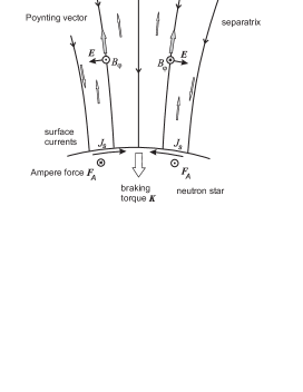
Figure 5: Schematic view of the axisymmetric polar cap showing magnetospheric current density (open arrows), surface currents, Ampére force on surface currents, and braking torque. Here only the symmetric current $i_{\rm s}$ is present. Taken from Beskin (1999).

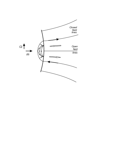
Figure 6: For the orthogonal rotator only antisymmetric current $i_{\rm a}$ (i.e., the current having different direction in the north and south parts of the polar cap) takes place. The structure of the surface currents within the polar cap and along the separatrix is also shown. Taken from Beskin et al. (2013).

The braking torque ${\bf K}$ of the Ampère force results in the following time evolution of the angular velocity $\Omega$ and the inclination angle $\chi$:

$$I_{\rm r}\,\dot{\Omega} = K_{\parallel}\cos{\chi}+K_{\perp}\sin{\chi},$$ (5)

$$I_{\rm r}\Omega\,{\dot{\chi}} = K_{\perp}\cos{\chi}-K_{\parallel}\sin{\chi},$$ (6)

where two components of the torque ${\bf K}$ parallel and perpendicular to the magnetic dipole ${\bf m}$ can be written in the form (Beskin et al., 1993)

$$K_{\parallel} = -c_{\parallel}\frac{B_{0}^{2}\Omega^{3}R^{6}}{c^{3}}i_{\rm s},$$ (7)

$$K_{\perp} = -c_{\perp}\frac{B_{0}^{2}\Omega^{3}R^{6}}{c^{3}}\left(\frac{\Omega R}{c}\right)i_{\rm a}.$$ (8)

Here the coefficients $c_{\parallel}$ and $c_{\perp}$ are factors of the order of unity dependent on the profile of the longitudinal current and the form of the polar cap.

The scalar current from the polar cap $i$ has been divided into symmetric and antisymmetric contributions, $i_{\rm s}$ and $i_{\rm a}$, depending upon whether the direction of the current is the same in the north and south parts of the polar cap, or opposite. For an axisymmetric rotating neutron star ($\chi=0$, Figure 6), we have $i_{\rm a}=0$ and $i_{\rm s}=1$ (Goldreich & Julian, 1969). Conversely, for the orthogonal rotator (Figure 6) we have $i_{\rm s}=0$ and $i_{\rm a}=1$. Here we apply normalization to the Goldreich-Julian current, $I_{\rm GJ}=\pi R_{0}^{2}j_{\rm GJ}$, where $R_{0}\approx R(\Omega R/c)^{1/2}$ is the polar cap radius, and $j_{\rm GJ}=<|{\bf\Omega}\cdot{\bf B}|>/2\pi$ (with scalar product) is the mean current density within the polar cap. Note that for $i_{\rm s}\approx i_{\rm a}\approx 1$, (7) and (8) imply that:

$$K_{\perp}\sim\left(\frac{\Omega R}{c}\right)K_{\parallel}.$$ (9)

Therefore, $K_{\perp}\ll K_{\parallel}$. We will use these expressions in the following sections.

If we suppose that, in reality, the longitudinal current $j$ is determined by the local charge density $\rho_{\rm GJ}=-{\bf\Omega}\cdot{\bf B}/2\pi c$, and note that $\rho_{\rm GJ}$ is proportional to $\cos\chi$ in the vicinity of the polar cap, one can write down

$$i_{\rm s} = i_{\rm s}^{A}\cos\chi,$$ (10)

$$i_{\rm a} = i_{\rm a}^{A}\sin\chi.$$ (11)

Consequently, the relations (5)–(6) can be rewritten in the form

$$I_{\rm r}\dot{\Omega} = K_{\parallel}^{A}+[K_{\perp}^{A}-K_{\parallel}^{A}]\sin^{2}\chi,$$ (12)

$$I_{\rm r}\Omega{\dot{\chi}} = [K_{\perp}^{A}-K_{\parallel}^{A}]\sin\chi\cos\chi.$$ (13)

As we see, both expressions contain the factor $[K_{\perp}^{A}-K_{\parallel}^{A}]$. This implies that the sign of $\dot{\chi}$ is given by the $\chi$-dependence of the energy losses (Philippov et al., 2014). In other words, the inclination angle $\chi$ will evolve to $90^{\circ}$ (to counter-alignment) if the total energy losses decrease for larger inclinational angles, and to co-alignment if they increase with inclination angle.

Because the plasma filling the pulsar magnetosphere is secondary (in other words, it is produced by the primary particles accelerated by the longitudinal electric field), at any point out to the light cylinder, the energy density of the electromagnetic field must be much larger than the energy density of the magnetospheric plasma. For the same reason, energy transport is given by the Poynting vector (see Figure 6).

Figure 7: The Michel split-monopole solution, in which electric field $E_{\theta}$ has magnitude equal to the toroidal magnetic field $B_{\varphi}$. This solution requires a conducting current sheet, to close electric currents (outlined arrows). Taken from Beskin (1999).

Figure 8: Magnetospheric structure in the model of Contopoulos et al. (1999). The last open field line is assumed to coincide with the equator.

4.2 Split-Monopole Model

The remarkable analytical solution found by Michel (1973) serves to illustrate the transport of energy by Poynting flux. In the force-free approximation, when massless charged particles move radially with the velocity of light, and with the Goldreich-Julian current density $j_{\rm GJ}=\rho_{\rm GJ}c$, a split-monopole magnetic field is the exact solution to the Maxwell’s equations, both inside and beyond the light cylinder (see Figure 8). The monopolar magnetic field is split so that the magnetic flux converges in the southern hemisphere and diverges in the northern one. In this solution, Ampère forces from longitudinal currents along magnetic field lines, and from corotation currents from rotating charge density, are fully compensated.

In the Michel split-monopole solution, the electric field ${\bf E}$ has only a $\theta$-component, and is equal in magnitude to the toroidal component of the magnetic field:

$$B_{\varphi}=E_{\theta}=-B_{0}\left(\frac{\Omega R}{c}\right)\frac{R}{r}\sin\theta.$$ (14)

At distances larger than the light cylinder radius, this magnetic field becomes larger than the poloidal magnetic field $B_{\rm p}=B_{0}(R/r)^{2}$. On the other hand, in this solution the total magnetic field remains larger than the electric field everywhere, so that the fields form electromagnetic waves only at infinity.

Because magnetic flux converges in the lower hemisphere and diverges in the upper one in the split-monopole solution, a current sheet must lie in the equatorial plane (see Figures 8, 8). This sheet closes the longitudinal electric currents elsewhere in the magnetosphere. This structure of the magnetic field and current sheet has been confirmed numerically (Contopoulos et al., 1999; Ogura & Kojima, 2003; Gruzinov, 2005; Komissarov, 2006; McKinney, 2006; Timokhin, 2006).

Using Eqn. (14), one easily finds that the Poynting vector ${\bf S}=(c/4\pi){\bf E}\times{\bf B}$ is:

$$S(\theta)=\frac{B_{0}^{2}c}{4\pi}\left(\frac{\Omega R}{c}\right)^{2}\frac{R^{2}}{r^{2}}\sin^{2}\theta.$$ (15)

This implies that the energy flux is concentrated near the equatorial plane. This $\theta$-dependence of the energy flux is used by many authors (Bogovalov & Khangoulyan, 2002; Komissarov & Lyubarsky, 2003). On the other hand, at large distances $r\gg R_{\rm L}$, Ingraham (1973) and Michel (1974) found another asymptotically radial solution, with $E_{\theta}(\theta)=B_{\varphi}(\theta)$, resulting in a radial Poynting vector with arbitrary $\theta$-dependence. In all of these solutions, the relation

$$S(\theta)\propto B_{r}^{2}(\theta)\sin^{2}\theta$$ (16)

is valid.

Bogovalov (1999) generalized the split-monopole model, showing that in the force-free approximation the “inclined split monopole field” is a solution of the problem as well. In this solution,

$$B_{\varphi} = E_{\theta}=-B_{0}\left(\frac{\Omega R}{c}\right)\frac{R}{r}\sin\theta\,{\rm sign}{\rm\Theta}$$ (17)

and $B_{\rm p}=B_{0}(R/r)^{2}\,{\rm sign}{\rm\Theta}$, where

$${\rm\Theta}=\sin\chi\sin\theta\sin(\varphi-\Omega t+\Omega r/c)+\cos\chi\cos\theta.$$ (18)

In this case, within the cones  $\theta<\pi/2-\chi$, $\pi-\theta<\pi/2-\chi$ around the rotation axes, the electromagnetic field is not time dependent; whereas in the equatorial region, the electromagnetic fields change the sign at the instant ${\rm\Theta}=0$. In other words, the condition ${\rm\Theta}=0$ defines the location of the current sheet. We stress that the expression (18) for the shape of the current sheet remains true for the other radial asymptotic solutions, with $E_{\theta}(\theta)=B_{\varphi}(\theta)$ but arbitrary $\theta$-dependence, as well (Arzamasskiy et al., 2015a). Numerical simulations obtained recently for the oblique force-free rotator confirm this conclusion as well (Spitkovsky, 2006; Kalapotharakos & Contopoulos, 2009; Kalapotharakos et al., 2012; Tchekhovskoy et al., 2013; Philippov et al., 2014).

4.3 Magnetohydrodynamic Models

As was already stressed, recently numerical simulations have become possible that can simulate the structure of plasma-filled magnetospheres from first principles. Contopoulos et al. (1999) found an iterative way to do this and obtained the first solution for an aligned force-free pulsar magnetosphere that extended out to infinity (see Figure 8). Their results were subsequently verified by other groups within force-free and magnetohydrodynamic (MHD) approximations (e.g., Gruzinov 2005; Timokhin 2006; McKinney 2006; Komissarov 2006; Parfrey et al. 2012; Ruiz et al. 2014) as well as using particle-in-cell (PIC) approach (Philippov & Spitkovsky, 2014; Chen & Beloborodov, 2014; Cerutti et al., 2014; Belyaev, 2014).

Spitkovsky (2006) carried out the first 3D, oblique pulsar magnetosphere simulations. Using the force-free approximation, he found that pulsar spindown luminosity increases with increasing obliquity angle, $\chi$, which is the angle between the rotational and magnetic axes. The spindown obtained in such force-free and MHD models is well-described by

$$W_{\rm tot}=W_{\rm aligned}(1+\sin^{2}\chi),$$ (19)

where $W_{\rm aligned}=m^{2}\Omega^{4}/c^{3}$ is the spindown luminosity of an aligned plasma-filled pulsar magnetosphere, and $m=B_{0}R^{3}/2$ is the magnetic dipole moment of the pulsar. More recently, these results were confirmed using time-dependent 3D force-free (Kalapotharakos & Contopoulos, 2009; Pétri, 2012; Kalapotharakos et al., 2012), MHD (Tchekhovskoy et al., 2013), and PIC (Philippov et al., 2014) studies. Figure 9 shows a vertical slice through the results of a 3D MHD simulation of an oblique pulsar magnetosphere with obliquity angle $\chi=60^{\circ}$. One can clearly see the closed zone that extends out to the light cylinder located at $|x|=R_{\rm LC}$, beyond which starts a warped magnetospheric current sheet, across which all field components undergo a jump. The structure of this current sheet is presently poorly understood, in particular it is not known if in the perfect conductivity limit the magnitude of the magnetic field in the sheet vanishes.

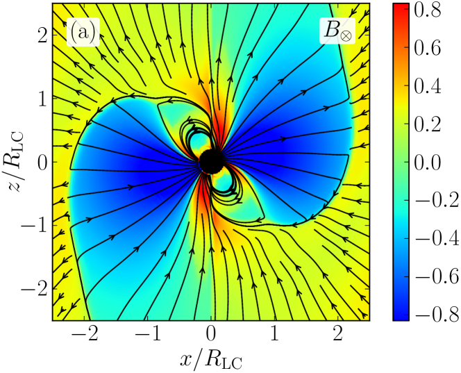
Figure 9: Slice through the $\vec{m}{-}\vec{\Omega}$ plane of a relativistic MHD simulation of an oblique pulsar magnetosphere (obliquity angle $\chi=60^{\circ}$) taken after $3$ rotations. Solid lines show field lines as traced in the image plane. Into-the–plane magnetic field component, $B_{\otimes}$, is shown with color (red – into plane, blue – out of plane). Taken from Tchekhovskoy et al. (2013).

What causes this increase of spindown luminosity with the increase of pulsar obliquity? It turns out that there are two factors: (i) an increase in the amount of open magnetic flux, which accounts for about $40$% of the increase, and (ii) redistribution of open magnetic flux toward the equatorial plane of the pulsar magnetosphere, which accounts for the remaining $60$%.

In fact, the spindown trend (19) can be reproduced via a simple toy model. Suppose that the magnetic field that reaches the light cylinder in an oblique rotator, with inclination angle $\chi$, retains the dipolar structure at $r=r_{0}\gg R_{\rm LC}$,

$$B_{r}=\frac{B_{0}r_{0}^{2}}{r^{2}}\sin\theta_{\rm m},$$ (20)

where $\theta_{\rm m}$ is the magnetic colatitude, or the angle away from the magnetic axis,

$$\theta_{\rm m}=\arccos(\sin\chi\sin\theta\cos\varphi+\cos\theta\cos\chi).$$ (21)

How would the pulsar spindown change if we kept the total open magnetic flux, $\Phi_{\rm open}=\pi r_{0}^{2}B_{0}$, fixed, and inclined the pulsar, i.e., increased $\chi$? To find this out, let us first compute the angular distribution of $\varphi$-averaged $B_{r}^{2}$:

$$\langle B_{r}^{2}\rangle_{\varphi}=B_{0}^{2}(0.5\sin^{2}\chi\sin^{2}\theta+\cos^{2}\theta\cos^{2}\chi).$$ (22)

Now, making use of the fact that $B_{\varphi}\approx E_{\theta}=-B_{r}\Omega r\sin\theta/c$ and the radial Poynting flux is $S_{r}=cE_{\theta}B_{\varphi}/4\pi\approx(B_{r}\Omega r\sin\theta)^{2}/4\pi c$, we obtain (Tchekhovskoy et al., 2015):

$$W_{\rm toy}(\chi)=\iint S_{r}\,{\rm d}\omega=\frac{\Omega^{2}\Phi_{\rm open}^{2}}{7.5\pi^{2}c}(1+\sin^{2}\chi),$$ (23)

where the integral is over, e.g., a sphere of radius $r_{0}$. Clearly, if the total magnetic flux $\Phi_{\rm open}$ is held constant, the nonuniformity in the surface distribution of magnetic flux causes an enhancement in spindown losses at higher inclination angles, consistent with the numerical simulations (see Eqn. 19). In the simulations, we find that the magnetic flux itself is an increasing function of $\chi$, $\Phi_{\rm open}\propto(1+0.2\sin^{2}\chi)$, so the two effects – of the non-uniformity of the open magnetic flux and the change in the amount of open magnetic flux – have very similar inclination-dependences.

In reality, the structure of the plasma-filled magnetosphere is of course more complex than given by Eqn. (20), but the qualitative effect is the same: the inclination of the magnetic axis relative to the rotational axis leads to the shift of the peak of $|B_{r}|$ away from the axis and toward the equatorial plane and an increase in the spindown luminosity (Tchekhovskoy et al., 2015).

More recently, PIC models have been developed and, in those cases when the magnetospheric polar cascade is efficiently operating and is able to fill the magnetosphere with abundant plasma, are in agreement in the amount of spindown and large-scale dissipation as in MHD simulations (see e.g. Philippov & Spitkovsky 2014; Chen & Beloborodov 2014; Cerutti et al. 2014; Belyaev 2014; Philippov et al. 2014). Interestingly, if a mechanism of pair formation operates only near the surface of the star, aligned pulsar magnetospheres in PIC simulations do not reach a force-free state (Chen & Beloborodov, 2014). In fact, PIC simulations, into which simplified physics of the polar cascade was included, show the development of the polar cascade and of a force-free–like magnetosphere only for high inclinations, $\alpha>40^{\circ}$ (Philippov et al., 2014).

5 Observations: Energy Loss from Pulsars

5.1 Spindown

In principle, the time rate of change of pulse period $\dot{P}$ is easy to measure. Because individual pulses can be numbered, period and period derivative are among the fundamental parameters of a timing model. Period derivative is easily associated with the loss of rotational kinetic energy via electromagnetic radiation and particle wind. The Larmor formula for magnetic dipole radiation then directly associates energy loss with the magnetic moment of the neutron star. This provides a characteristic scale.

Pulsars with periods longer than a fraction of a second show timing noise: random variations of pulse arrival time that change slowly with time (Helfand et al., 1980). These variations are most extreme for the young Crab and Vela pulsars (Boynton et al., 1972; Lyne & Graham-Smith, 1998; Scott et al., 2003; Dodson et al., 2007). Among millisecond pulsars, B1937+214 shows timing noise, but other millisecond pulsars may not (Kaspi et al., 1994; Cognard et al., 1995).

Several pulsars show clear variations in spindown rate associated with changes in pulse properties. The radio pulsars B1931+24, J1832+0029, and J1841-0500 intermittently switch between an “on” radio-loud state in which they appear as ordinary radio pulsars, and an “off” state in which no radio emission is detected. The spin-down rate is higher in the “on” state than the “off” state, by a factor of $f_{{\rm on}\rightarrow{\rm off}}=\dot{P}_{\rm on}/\dot{P}_{\rm off}\approx 1.5$ for B1931+24 (Kramer et al., 2006) and J1832+0029 (Lyne, 2009), and $f_{{\rm on}\rightarrow{\rm off}}\approx 2.5$ for J1841$-$0500 (Camilo et al., 2012). The gamma-ray pulsar J2021+4026 Allafort et al. (2013) displays two states with intensities different by 20% and with distinct pulse profiles, each associated with a different spindown rate: $f_{{\rm on}\rightarrow{\rm off}}=1.04$. Pulsar B0919+06 shows quasiperiodic variations between two states with different spindown rates and different pulse profiles (Perera et al., 2015). Lyne et al. (2010) propose that the phenomenon of intermittency is quite general: they find that timing noise for six pulsars can be expressed as the superposition of two states, characterized by distinct pulse profiles and spindown rates, with rather rapid changes between states. From these discussions it is clear that magnetospheric structure affects spindown, as one would suspect from theoretical considerations discussed in Section 2.3 above.

Kramer et al. (2006) (see also Beskin & Nokhrina, 2007) proposed that two distinct magnetospheric states lead to the observed difference in spindown rates. They associated the “off” state with a magnetosphere depleted of charge, and the “on” state with magnetospheric currents sufficient to produce the observed change in spindown. Li et al. (2012) observe that the simplest model for the “on” state is the force-free magnetosphere (Spitkovsky, 2006), which exhibits spindown rates at least three times that of a vacuum dipole. They suggest a modified picture where the “on” state is the force-free magnetosphere, and the “off” state has no charge on open field lines, but carries the Goldreich-Julian charge on closed field lines. This leads to ratios $f_{{\rm on}\rightarrow{\rm off}}=1.2$ to $2.9$ for inclination angles of $\chi>30^{\circ}$. Smaller inclinations lead to larger $f_{{\rm on}\rightarrow{\rm off}}$.

5.2 $\sigma$-Problem

Thus, we see that all analytical and numerical force-free models of the pulsar magnetosphere demonstrate the existence of an almost-radial highly-magnetized wind, flowing outward from the pulsar magnetosphere. On the other hand, observations show that most energy far from the neutron star must be carried by relativistic particles (Kennel & Coroniti, 1984a, b). For example, the analysis of the emission from the Crab Nebula in the shock region located at a distance of $\sim 10^{17}$ cm from the pulsar in the region of interaction of the pulsar wind with the supernova remnant definitely shows that the total flux $W_{\rm em}$ of the electromagnetic energy in this region is no more than $\sim 10^{-3}$ of the particle energy flux $W_{\rm part}$. Thus, in the asymptotically far region of pulsar models, the Poynting flux must be completely converted into an outgoing particle flux before reaching the reverse shock at distances of $\sim 0.1$ pc. Axisymmetric numerical models of jets from radio pulsars are constructed exactly under this assumption (Kirk et al., 2009, and references therein).

The transformation from Poynting flux to particles apparently occurs much closer to the neutron star, at distances comparable to the size of the light cylinder. This is evidenced by the detection of variable optical emission from companions in some close binary systems involving radio pulsars (Fruchter et al., 1988; Kulkarni et al., 1988; Fruchter et al., 1990; Ryba & Taylor, 1991; Stappers et al., 1996; Roberts, 2011; Pallanca et al., 2012; Romani et al., 2012; Kaplan et al., 2013; Breton et al., 2013). This variable optical emission with a period equal exactly to the orbital period of the binary can be naturally related to the heating of the companion’s surface facing the radio pulsar. It was found that the energy reradiated by the companion star almost matches the total energy emitted by the radio pulsar into the corresponding solid angle. Clearly, this fact cannot be understood either in the magnetic-dipole radiation model or by assuming a Poynting-dominated strongly-magnetized outflow, since the transformation coefficient of a low-frequency electromagnetic wave cannot be close to unity. Only if a significant fraction of the energy is related to the relativistic particle flux can the heating of the star’s surface be effective enough. Moreover, eclipses of the double-pulsar system show effects of the particle wind from one object impinging upon (Lyne et al., 2004; Jenet & Ransom, 2004; McLaughlin et al., 2004; Lyutikov, 2004; Demorest et al., 2004). Therefore, the so-called $\sigma$-problem — the question as to how the energy can be converted from electromagnetic fields to particles in the pulsar wind — remains one of great unsolved problems of modern astrophysics. We note that the $\sigma$-problem appears to be rather general and in addition to neutron-star powered outflows it applies to black-hole powered, collimated outflows known as astrophysical jets, such as in the magnetically-arrested disk (MAD) scenario (Tchekhovskoy et al., 2011; Tchekhovskoy & McKinney, 2012; Zamaninasab et al., 2014; Zdziarski et al., 2014; Ghisellini et al., 2014; Tchekhovskoy, 2015). Theoretical models suggest that the jets accelerate roughly up to the equipartition between the magnetic and kinetic energies, beyond which the acceleration slows down dramatically, locking in a substantial fraction of energy in the magnetic form (Tchekhovskoy et al. 2009; Komissarov et al. 2009; Lyubarsky 2010; however, see Tchekhovskoy et al. 2010).

6 Theory: Polarization and Refraction of Radio Emission

6.1 Polarization

Pulsar emission is usually highly linearly polarized, with a small fraction of circular polarization. Like the mean profile, the profiles in polarization states are stable and are characteristic of the pulsar. This long-term stability of the mean properties indicates that the pulse arises as a cut through a radiation cone, with properties that are set by stable properties of the underlying neutron star. It is widely assumed that the polarization is determined by magnetic fields in or above the emission region. Those magnetic fields, in turn, are anchored in the solid crust of the neutron-star (Manchester, 1995).

Rapid swings of the position angle of linear polarization through the pulse, first observed in the Vela pulsar by Radhakrishnan et al. (1969), suggest that a vector fixed in the frame of the rotating star influences the direction of linear polarization, a geometric inference known as the rotating-vector model. Radhakrishnan & Cooke (1969) proposed that this vector is the magnetic pole of the pulsar’s nearly-dipolar magnetic field; this physical interpretation is known as the magnetic-pole model.

Radiotelescopes can measure polarization properties of individual pulses for a number of strong pulsars. Such studies indicate the presence of orthogonal modes, with polarization differing by $90^{\circ}$, and intensities varying from pulse to pulse (Manchester et al., 1975; Backer et al., 1976; Cordes et al., 1978; Backer & Rankin, 1980; Stinebring et al., 1984a, b; McKinnon, 2003). For most pulsars, present radiotelescopes can determine only average polarization properties; nevertheless the presence of two competing orthogonal modes can explain the observed departures from the characteristic pattern, for most of these weaker pulsars. Thus, the rotating-vector model, with two orthogonal linearly-polarized modes, successfully describes the characteristic swing of the angle of polarization with pulse phase for most pulsars, across a wide range of pulsar parameters and despite observational selection effects (Rankin, 1983, 1986; Lyne & Manchester, 1988). The two modes are usually interpreted as the X-mode, with wave electric field perpendicular to stellar magnetic field ($E_{W}\perp B_{0}$); and the O-mode, with a component of electric field parallel to stellar field ($E_{W}||B_{0}$). Both modes appear to be present, at some level, for all radio pulsars.

Work to model the polarization properties of pulsars in more detail, including the circular-polarized profile, have led to mapping of the polarization properties on the Poincaré sphere describing the Stokes parameters (McKinnon, 2009; Chung & Melatos, 2011a, b). These show a rich variety of patterns, with greater modulation of polarization being indicative of more complex patterns. Analysis of these patterns suggest emission, or refractive scattering within the pulsar’s light cylinder. For some pulsars, the emission, or reprocessing region is inferred to lie at altitudes of 10 to 40% of the light-cylinder radius.

6.2 Rotating Vector Model

The standard relation for the rotating vector model describes variation of the position angle of polarization $\psi$ in the mean profile, under the assumption that the the hollow-cone model is valid. In other words, it assumes that all absorption is absent, and that the magnetic field is dipolar in the emission region, precisely where the polarization is determined. This relation takes the form:

$$\psi={\rm arctan}\left(\frac{\sin\chi\sin\phi}{\sin\chi\cos\zeta\cos\phi-\sin\zeta\cos\chi}\right),$$ (24)

Here, once again, $\chi$ is the inclination angle of the magnetic dipole to the rotation axis, $\zeta$ is the angle between the rotation axis and the direction toward the observer, and $\phi$ is the phase of the pulse. Figure 10 illustrates the geometry. Equation (24) has been used for many years in estimating the pulsar inclination angle, which is a very important parameter for determining the structure of the magnetosphere. Aberration and retardation effects (Blaskiewicz et al., 1991) have been included in only some studies (Mitra & Li, 2004; Krzeszowski et al., 2009).

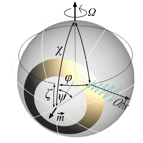
Figure 10: Geometry for the rotating vector model. The emission surface is shown as a golden band. As the pulsar rotates, the line of sight to the observer traverses a circle of constant latitude, producing an observed pulse each time the emission surface crosses the line of sight. The dipolar magnetic field, projected onto the radius of the emission surface, radiates from the magnetic pole $\vec{m}$. The instantaneous polarization of the observed radiation is parallel to the field lines, at position angle $\psi$ at the observer.

The rotating vector model, extended further with the “hollow cone” model, is based on the following three assumptions (see, e.g., Manchester & Taylor (1977)): the formation of polarization occurs at the point of emission; radio waves propagate along straight lines; and cyclotron absorption can be neglected. But all these assumptions turn out to be incorrect. Barnard & Arons (1986) showed that in the innermost regions of the magnetosphere, the refraction of one of the normal modes is significant. After publication of the work of Mikhailovskii’s group (Mikhailovskii et al., 1982), it became clear that cyclotron absorption can significantly affect the radio emission intensity. The influence of the magnetosphere plasma on variation of the polarization of radio emission propagating in the internal regions of the magnetosphere also must not be neglected (Petrova & Lyubarskii, 2000).

The “limiting polarization” is the most important effect of magnetospheric propagation. Radio emission in the region of dense plasma consists of a superposition of normal modes: in particular, the principal axes of the polarization ellipse must remain aligned with the magnetic-field direction in the picture plane. Polarization in the vacuum region is independent of magnetic field. Hence, between the two lies a transition layer, past which the polarization is no longer affected by the magnetospheric plasma. For typical parameters of the pulsar magnetosphere, the formation of polarization occurs not at the emission point but at a distance of about $0.1R_{\rm L}$ from it (Cheng & Ruderman, 1979; Barnard, 1986). Taking this effect into account should also explain the observed fraction of circular polarization of the order of (5-10)%. Therefore, a consistent theory of radio wave propagation in the magnetosphere is required for a quantitative comparison of theoretical results on radio emission with observational data.

6.3 Propagation effects

At present, the theory of radio wave propagation in the magnetosphere of a pulsar can be considered to provide the necessary precision (Petrova, 2006; Wang et al., 2010; Beskin & Philippov, 2011, 2012; Kravtsov & Orlov, 1980). Four normal modes exist in the magnetosphere (Beskin et al., 1993; Lyne & Graham-Smith, 1998). Two of them are plasma modes and two are electromagnetic, which are capable of departing from the magnetosphere. An extraordinary wave (the X-mode) with the polarization perpendicular to the magnetic field in the picture plane propagates along a straight line, while an ordinary wave (the O-mode) undergoes refraction and deviates from the magnetic axis. An important point here is that for typical magnetosphere parameters, refraction occurs at distances up to $0.1R_{\rm L}$, i.e., it can be considered separately from the cyclotron absorption and the limiting polarization. As shown in Figure 11, the pulsar B0329$+$54 shows both X- and O-modes, with the O-mode displaying deviations from the rotating-vector model because of refraction (Edwards & Stappers, 2004).

Based on the Kravtsov & Orlov (1980) method, Beskin & Philippov (2012) have used such a theory of wave propagation in a realistic pulsar magnetosphere, taking corrections to the dipole magnetosphere into account (based on the results obtained by numerical simulation in Spitkovsky (2006)), together with the drift of plasma particles in crossed electric and magnetic fields, and a realistic particle distribution function. The theory developed allows dealing with an arbitrary profile of the spatial plasma distribution, which may differ from the one in the hollow-cone model, because precisely the inhomogeneous plasma distribution leads to the characteristic ‘patchy’ directivity pattern (Rankin, 1990).

The main result consists in the prediction of a correlation between the sign of the circular polarization (the Stokes parameter $V$) and the sign of the derivative of the change in the polarization of the position angle, $\psi$, along the profile, ${\rm d}\psi/{\rm d}\phi$, where $\phi$ is the phase of the radio pulse. For the ordinary mode, these signs must be opposite to each other, while for the extraordinary mode, they must coincide. Figure 11 shows this pattern as well. As was noted, refraction of the ordinary wave leads to a deviation of beams from the rotation axis, and therefore the ordinary wave pattern should be broader than for the extraordinary wave. In the case of the ordinary mode, double radio emission profiles should mainly be observed, while single profiles should be observed in the case of the narrower extraordinary mode (Beskin et al., 1993).

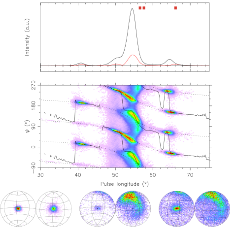
Figure 11: Polarization properties of the strong pulsar B0329$+$54. Upper panel: Average pulse profile, showing both total (black) and polarized (red) intensity plotted with pulse phase. Middle panel: Histogram of angle of linear polarization $\psi$ plotted with pulse phase. Dotted curves show polarization for the rotating-vector model. Red shows most common values, ranging through less-common green, blue, and violet, to white for not observed. One linear polarization (presumably X) tracks the rotating-vector model well, while the other (presumably O) shows large variations in polarization and timing. Lower panels: Polarization parameters on the Poincaré sphere, for the 3 intervals of pulse phase indicated by red boxes at in the upper left panel. Each pair of disks shows 2 hemispheres. Linear polarization lies on the equator; pure right circular polarization is at the upper pole, pure left circular at the lower. This image from Edwards & Stappers (2004) is reproduced by courtesy of B. W. Stappers.

As was shown by Andrianov & Beskin (2010), observations fully confirm the prediction of correlation between signs of $V$ and ${\rm d}\psi/{\rm d}\phi$. The analysis used over 70 pulsars with well-traced variation of the position angle and the sign of the circular polarization $V$, chosen from reviews of pulse profiles Weltevrede & Johnston (2008); Hankins & Rankin (2010). Table 1 presents the results of the analysis. Pulsars with opposite signs of the derivative ${\rm d}\psi/{\rm d}\phi$ and the Stokes parameter $V$ were placed in class O, while those with identical signs were placed in class X. As can be seen from the Table, most of the pulsars exhibiting a double-peaked (index D) profile indeed correspond to the ordinary wave, while most of the pulsars with single-peaked profiles (index S) correspond to the extraordinary wave. Moreover, the average width of the radiation pattern for ${\rm O_{D}}$ pulsars is indeed about two times larger than the average width of the radiation pattern for ${\rm X_{S}}$ pulsars. For the pulse width, the analysis used the width at the 50% intensity level $W_{50}$, normalized to the pulsar period $P$. The existence of a certain number of pulsars of classes ${\rm O_{D}}$ and ${\rm X_{S}}$ should not give rise to surprise, because for central passage through the directivity pattern, independently of whether it corresponds to the O-mode or to the X-mode, a double-peaked profile should be observed, while for lateral passage, a single-peaked profile should be observed.

Table 1: Statistics of pulsars with known circular polarization V and variation of position angle $\psi$.

Polarization Mode	O			X
Profile Type	Single	Double		Single	Double
Class	OS	OD		XS	XD
Number of Pulsars	6	23		45	6
Normalized Pulse Widtha	6.8$\pm$ 3.1	10.7$\pm$ 4.5		6.5$\pm$ 2.9	5.3$\pm$ 3.0
$a$ Normalized pulse width given as: $\sqrt{P}W_{50}$ (s1/2 deg)

Accurately taking propagation effects into account, Andrianov & Beskin (2010); Beskin & Philippov (2011) showed that such a variation of the position angle can be realized only under conditions of low plasma density or high mean particle energy. They found significant deviations from the standard relation of the rotating vector model (Eq. 24) were obtained in the case of quite reasonable parameters that satisfy models for particle production: for example, a multiplicity $n_{\rm e}/n_{\rm GJ}\sim 10^{4}$ and an average Lorentz factor $\gamma\sim 50$.

7 Observations: Polarization and Pulsar Size

7.1 Pulsar Emission Region Size and Shift

The radio emission regions of pulsars lie within the light cylinder, and so have angular sizes from Earth of nanoarcseconds or less. Resolving such an angle at radio wavelengths requires an instrument with an aperture approaching an AU, beyond the capabilities of even the longest VLBI baselines (Kardashev et al., 2013). However, radio-wave scattering by the dilute, turbulent interstellar plasma yields the required angular resolution and offer some of the information provided by a lens of that aperture.

Interstellar scattering affects almost all astrophysical sources at decimeter wavelengths, and for many at shorter wavelengths. For most radio pulsar observations, scattering is “strong” in the sense that paths contributing to the electric field measured at the observer differ in length by many wavelengths. Hence, these paths behave like a corrupt lens (Gwinn et al., 1998). The angular extent on the sky of these paths, $\theta$, delineates the “scattering disk”. The scale of variation of the impulse-response function at the observer, $S_{\rm ISS}$, is the diffractive spot size of that aperture, $\sim\lambda/\theta$. (Here, the subscript “${\rm ISS}$” indicates “interstellar scattering”.) The scattering produces a random diffraction pattern in the observer plane with lateral scale $S_{\rm ISS}$. The effective resolution limit of the corrupt lens, at the source, is $MS_{\rm ISS}$, where the magnification factor $M=D/R$ is equal to the distance $D$ of the scattering material from the observer, divided by its distance $R$ from the source. Interstellar scattering does not remove information from the pulsar signal; rather, it adds a great deal of information about the paths taken. The challenge facing the observer is to extract the spatial information about the source from the scattered pulsar signal.

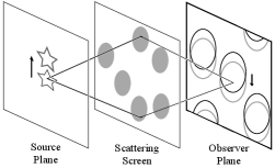
Figure 12: Geometry for studies of pulsar structure by scattering. Radiation emitted by the pulsar at left travels to the scattering screen, where fluctuations in plasma density change its phase. The radiation arrives at the plane of the observer at right from along many paths, with different phases and amplitudes. Interference among paths produces a random diffraction pattern in the plane of the observer. When the source shifts to a different position, because of either proper motion or a rotational shift in the location of the pulsar emission region, the phases of the paths are modified, to produce a reflex motion of the diffraction pattern in the plane of the observer.

Studies of the sizes of pulsar emission regions using interstellar scattering fall into two categories. One category relies upon the fact that if the emission point of the pulsar shifts across the pulse, the random image in the plane of the observer will undergo a reflex shift, as illustrated in Figure 12. Proper motion causes a similar shift, but over time spans of many pulses. Correlation of the scintillation spectrum across pulse phases with later or earlier times yields the shift of the emission point (Backer, 1975; Cordes et al., 1983; Wolszczan & Cordes, 1987; Smirnova et al., 1996; Gupta et al., 1999; Pen et al., 2014).

A second category invokes the decreased modulation for scintillation of an extended source. (“Stars twinkle, planets do not.”) The depth of modulation reveals the size of the emission region (Cohen et al., 1966; Readhead & Hewish, 1972; Hewish et al., 1974; Gwinn et al., 2012b; Johnson et al., 2012b). More precisely, source size affects the distribution of flux density for a scintillating source. In strong scattering many different paths, with lengths differing by many radians of phase, contribute to the electric field measured at a point in the observer plane. The observer implicitly sums over these paths, so that the observed phase and amplitude have the character of a random walk. The optics of this effect are similar to those of the reflex shift: different parts of the source produce shifted, incoherent diffraction patterns at the observer, who sums over them. Thus, finite source size affects the distribution of intensity at one antenna, or that of correlated flux density between the two antennas of an interferometer, principally by shifting the lowest and highest intensities toward the central part of the distribution (Scheuer, 1968; Gwinn, 2001; Johnson & Gwinn, 2012a, 2013). For realistic observations, the contributions of background noise, and of the noiselike statistics of the source itself, must be taken into account (Gwinn et al., 2011, 2012a; Johnson & Gwinn, 2012a, 2013).

7.2 Observations

7.2.1 Size of the Vela Pulsar’s Radio Emission Region: $\lambda=18$ cm

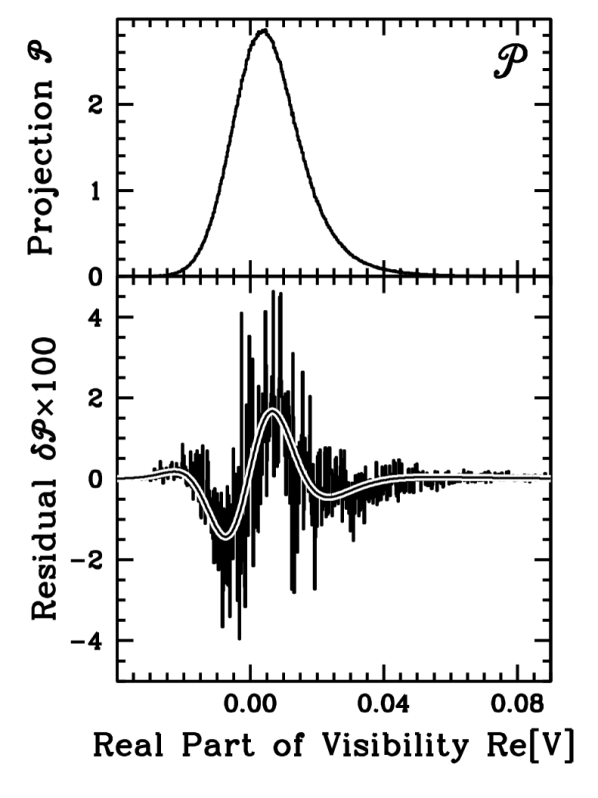
Figure 13: Observed distribution of visibility projected onto the real axis ${\mathcal{P}}$, in bins along the real axis. Upper: Observed distribution. Lower: Residuals to best-fitting model with zero size for the Vela pulsar at $\lambda=18$ cm. Curve shows difference of finite- and zero-size models. After Gwinn et al. (2012b).

Figure 14: Best-fitting amplitude (top panel) and source size $(kM\theta\sigma)$ (lower panel) plotted with pulse gate, for 4 gates in 6 spectral ranges. The model for the emission region assumes a circular Gaussian distribution of emission. After Gwinn et al. (2012b).

The fundamental observable of interferometry is visibility, the product of electric fields at a pair of antennas (Thompson et al., 2001). Because electric fields of all astrophysical sources are noiselike, this product must be averaged over some range of time and frequency. For a scintillating source, this averaging must be less than the scales of variation of the scintillation pattern with time and frequency, to preserve the variation of visibility from scintillation (Gwinn et al., 2000).

For a scintillating point source, in the absence of noise, the distribution of interferometric visibility is sharply peaked at the origin (Gwinn, 2001). The effect of a small but finite emission size is to soften the sharp peak, shift it from the origin, and narrow the distribution. As compared with a point-source model, the finite-size distribution without noise peaks at larger real part, but has lower probability density at large and small visibility, for the same average flux density (or equivalently, the same mean visibility).

Noise broadens the distribution of visibility. Although noise blurs the distributions and their projections, the difference of point-source and finite-size distributions persists, with a characteristic W-shaped signature, as Figure 14 shows. To compare with pulsar observations, we must also incorporate the effects of intrinsic variability. Rapid variability modifies the noise statistics, while variability over longer times broadens the distribution (Gwinn et al., 2011, 2012a). Consequences of these effects differ from those of emission size.

Because finite size narrows the distribution of visibility, and noise broadens it, the difference of best-fitting models with finite size and zero size has a characteristic W-shaped signature. Figure 14 shows one example of a fit for a range early in the pulse. The characteristic W-shaped residual is evident, indicating the presence of a finite emission size. A model including one additional parameter, for finite size for the pulsar’s emission region, matches this residual accurately with significance exceeding 40$\sigma$. The inferred size of the emission region is 420 km. From fits to gates as a function of pulse phase, we find that the size of the pulsar emission region is large at the beginning of the pulse, declines to near zero size near the middle of the pulse, and then increases again to nearly 1000 km at the end of the pulse. The quoted sizes indicate the full width at half maximum of an equivalent circular Gaussian model.

Theoretical models of pulsar emission typically take their starting point in the geometrical models described above. Hakobyan & Beskin (2014) made theoretical calculations of the images of pulsars as a function of pulse phase, using generic expressions for the emission altitude and beam shape. They include effects of refraction by the magnetospheric plasma, and investigate emission heights up to 100$\times$ the radius of the neutron star. They find a characteristic U-shaped curve of the form seen in Figure 14. This form results from the greater curvature of field lines further from the magnetic pole, and the consequently greater set of loci that can emit in a given direction. Interestingly, they find that the size of the emission region is much larger than its shift over the course of a pulse. Yuen & Melrose (2014) investigate a similar model, and find that the shift of the emission region over a pulse is indeed small. They suggest from geometrical arguments that emission arises at altitudes of more than 10% of the light-cylinder radius. Lyutikov et al. (1999) comes to similar conclusions based on emission physics.

7.2.2 Size of the Vela Pulsar’s Emission Region at $\lambda=40$ cm from Nyquist-Limited Statistics

Figure 15: Observed and model PDFs of intensity for the subsets of pulses in the top and bottom decile by pulse intensity. Theoretical residual curves are completely determined by a single parameter, the source size. Plotted results correspond to a point source and a source that extends over 20 km; the latter is clearly inconsistent with the observed statistics. From Johnson et al. (2012b).

Figure 16: Inferred emission sizes of individual pulses at $\lambda=40$ cm. The size is displayed as a function of the single-pulse signal-to-noise ratios $S$; both linear polarizations are plotted. Because $S$ determines the standard error for each measurement to excellent accuracy, we omit error bars and instead show the expected $\pm 3\sigma$ errors about $\gamma_{s}=0$. We do not obtain a statistically significant detection of emission size for any pulse. From Johnson et al. (2012b).

The unique nature of pulsar emission allows an elegant solution to determination of the distribution of intensity of a variable, scintillating source: the formation of spectra that contain all single-pulse power. Such spectra require a Fourier transform of a data stream that spans the entire pulse, including any scatter-broadening. Without any averaging at all (that is, at the Nyquist limit of the data stream), such spectra show the influence of finite source size. Johnson & Gwinn (2012a) calculated the distribution of Nyquist-sampled spectra, for scintillating sources with and without effects of size, including the effects of averaging and temporal decorrelation. With knowledge of background noise from off-pulse spectra, the intensities of individual pulses, and the scintillation timescale, these statistics provide a measure of source size. A great strength of this technique is that it can measure size for individual pulses, or narrow classes of pulses.

Johnson et al. (2012b) used the Nyquist-sampled technique to find the size of the Vela pulsar at 40-cm wavelength, using baseband recording of the pulsar’s electric field, at the Green Bank Telescope. They found that the size was consistent with a pointlike source in all cases. The observational upper limit depended upon the set or subset of pulses analyzed. Figure 16 shows a typical example, the distribution of intensity for the brightest 10% of pulses, and for the weakest 10%. The distributions are normalized to the mean intensity in both cases, so differences arise from the difference in signal-to-noise ratio. The size is expressed in terms of the characteristic scales of interstellar scattering by the parameter $\gamma_{s}=\left(2\pi M\theta\sigma/\lambda\right)^{2}$. Here, $\theta$ is the angular broadening by interstellar scatter, and $\sigma$ is the size of a model Gaussian distribution of intensity at the source, both expressed as standard deviation. The observing wavelength is $\lambda$, and $M$ is the ratio of the distance of the observer from the scattering screen, to that of the pulsar from the screen. As the figure shows, both distributions are clearly inconsistent with a size as large as $\sigma_{\rm c}=20$ km, corresponding to a full-width at half-maximum of 47 km of an assumed circular Gaussian emission region. Figure 16 shows the size of the pulsar as measured in individual pulses, with a range of signal-to-noise ratios. From an fit to their full sample of pulses, they obtained a 3$\sigma$ upper limit of $\sigma_{\rm c}<4$ km (FWHM$<9$ km). These sizes are comparable to the size of the neutron star, and suggest a very concentrated emission region. Theory would suggest that the shift of the emission region is still smaller (Hakobyan & Beskin, 2014; Yuen & Melrose, 2014).

At face value, our results for the size of the emission region of the Vela pulsar at wavelengths of 18 and 40 cm appear inconsistent (Gwinn et al., 2012b; Johnson et al., 2012b)). How can the size of the emission region change by an order of magnitude, with a change of only 2$\times$ in observing wavelength? Longer wavelengths are thought to arise at higher altitudes, apparently exacerbating the discrepancy (Sturrock, 1971; Ruderman & Sutherland, 1975). Repeated observations have confirmed the observational results.

Refraction of a emergent double-peaked component at $\lambda=18$ cm may be responsible. At $\lambda=40$ cm the pulse profile contains a single “core” component, but at $\lambda=18$ cm an additional, double, “cone” component appears (Komesaroff et al., 1974; Kern et al., 2000; Johnson et al., 2012b). As discussed in Section 6.3, a double-peaked component indicates the presence of the O-mode, and the effects of refraction; whereas a single-peaked component indicates the X-mode and no refraction, and consequently a smaller size. Magnetospheric refraction might be stronger at the shorter wavelength Arons & Barnard (1986); Barnard & Arons (1986); Lyutikov & Parikh (2000); Hirano & Gwinn (2001); Hakobyan & Beskin (2014). This matches the observed pattern.

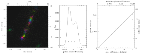
Figure 17: Left panel: Inferred image of the speckles that scatter pulsar B0834$+$06. Color is proportional to time delay, in a periodic hue map. This image becomes the celestial interferometer aperture, for imaging pulsar B0834$+$06. Center: Pulse profile, with 3 bins indicated. Right: Inferred shift of emission region with pulse phase. This image from Pen et al. (2014) is reproduced courtesy of U.-L. Pen.

7.2.3 Femtoarcsecond Astrometry of Pulsar B0834$+$06

Pen et al. (2014) extended the comparison of pulsar scattering patterns at different pulse phases. They model the scattering as the interference of a set of points at the screen, the “speckles”. Their method isolates the wavefields of each pair of interfering speckles. Interference of each pair of speckles acts as a 2-slit interferometer to cause the pulsar intensity observed at Earth to vary with a specific timescale and bandwidth. A shift of the position of the emission region of the pulsar, over the course of a pulse, causes a reflex shift of the interference pattern from each pair. Pen et al. inverted the very-long baseline interferometry observations of this pulsar by Brisken et al. (2010)to infer the structure of the speckles at the scattering screen, as shown in Figure 17.They use a holographic technique to partially descatter the data (see also Walker et al. (2008)). Their technique corrects for the phase of each speckle relative to its neighbors, and so effectively concentrates the power and boosts the signal-to-noise ratio. The application of this technique to PSR 0834+06 yields an astrometric determination of the phase shift across the pulse profile equivalent to an angular resolution of 150 picoarcseconds, or 10 km at the distance of the pulsar. This remarkable accuracy is comparable to the shift in position of the pulsar due to proper motion, over a single pulse. In particular, they found that the velocity of the radio image in the picture plane is about 1000 km s^-1, in good agreement with theoretical prediction (Hakobyan & Beskin, 2014).

8 Magnetic Axis Alignment

8.1 Theoretical Predictions for Motion of the Magnetic Axis

As was shown above, resulting from the MHD theory of the neutron star magnetosphere, the magnetospheric torque acting on the surface of a neutron star gives the positive factor $[K_{\perp}^{A}-K_{\parallel}^{A}]$ in (12)–(13) corresponding to the alignment evolution of the inclination angle. On the other hand, according to (9), this implies that the antisymmetric current $i_{\rm a}$ is to be large enough. E.g., for orthogonal rotator the longitudinal current $j$ is to be $10^{3}$–$10^{4}$ times larger than the local Goldreich-Julian one $j_{\rm GJ}^{{\rm loc}}={|\bf\Omega}{\bf B}|/2\pi$. Recent simulations of pair production in the inner gap (Timokhin & Arons, 2013) suggest that the microphysics of the cascade near the polar cap can support the large currents ($j\gg j_{\rm GJ}^{{\rm loc}}$) required by the global magnetospheric structure (it could be accompanied by an efficient heating of the polar cap). Similar results are obtained also by global, 3D PIC simulations of pulsar magnetospheres Philippov et al. (2014). In fact, force-free, MHD, and PIC simulations all find that even though for an orthogonal pulsar $j_{\rm GJ}$ essentially vanishes due to the midplane symmetry, the magnitude of the current flowing out along the open magnetic field lines is very similar to that of the aligned pulsar. The results of force-free and MHD simulations tell us that (Philippov et al., 2014),

$$K_{\parallel} =-K_{\rm aligned}\cos\chi,$$ (25)

$$K_{\perp} =-2K_{\rm aligned}\sin\chi,$$ (26)

where $K_{\rm aligned}=W_{\rm aligned}/\Omega=\mu^{2}\Omega^{3}/c^{3}$ is the spindown torque of an aligned rotator. Therefore,

$$I_{\rm r}\dot{\Omega} \approx-K_{\rm aligned}(1+\sin^{2}\chi),$$ (27)

$$I_{\rm r}\Omega{\dot{\chi}} \approx-K_{\rm aligned}\sin\chi\cos\chi.$$ (28)

Thus, the force-free and MHD simulation results suggest that pulsars tend to become aligned with time. This is not surprising in the context of previous discussion: pulsars tend to evolve toward the lowest luminosity state, e.g., toward the aligned state (see (19). Vacuum pulsars become aligned exponentially fast, even before they have a chance to spin down substantially, and generically end up with a period that is a few times their birth period. If most pulsars were born as millisecond rotators, this presents a problem in pulsar population synthesis studies, as this would imply that most pulsars would have millisecond periods, yet we observe many pulsars with periods of $\sim$second. In contrast, plasma-filled pulsars come into alignment much slower, as a power-law in time, $\chi\propto t^{-1/2}$, so both the spindown and alignment proceed at a similar rate (Philippov et al., 2014).

On the other hand, if there is some restriction of the value of the longitudinal current flowing through the polar cap (no numerical simulation has such a restriction), the situation can be different. Such an alternative model in which both symmetric and antisymmetric currents correspond to the local Goldreich-Julian value was considered by Beskin et al. (1983, 1993). They calculated the torque associated with the Ampére force arising from the interaction of the neutron star poloidal field with the surface currents (these currents close the longitudinal currents flowing in the region of open magnetosphere). One can prove by straightforward but cumbersome calculation that the two approaches are identical. This is a crucial assumption because pulsar spindown luminosity is proportional to the magnetospheric current squared.

For $i_{\rm a}\approx i_{\rm a}\approx 1$ equations (12)–(13) can be rewritten as

$$I_{\rm r}\dot{\Omega} \approx K_{\parallel}^{A}\cos^{2}\chi,$$ (29)

$$I_{\rm r}\Omega{\dot{\chi}} \approx K_{\parallel}^{A}\sin\chi\cos\chi;$$ (30)

for orthogonal rotator $\cos\chi<(\Omega R/c)^{1/2}$ we have

$$I_{\rm r}\dot{\Omega}\approx\left(\frac{\Omega R}{c}\right)K_{\parallel}^{A}.$$ (31)

As for $\cos\chi>(\Omega R/c)^{1/2}$ evolutionary equations (29)–(30) have an integral

$$\Omega\sin\chi={\rm const},$$ (32)

this model predicts the evolution of the inclination angle toward an orthogonal configuration. Thus, two theoretical models of the neutron star evolution give approximately identical predictions for the period derivative $\dot{P}$, but opposite ones for the evolution of the inclination angle $\chi$.

8.2 Observational Constraints on Evolution of Inclination Angle

Measurement of the rate of change of position angle with pulse phase at the center of the pulse $d\psi/d\phi$ yields only a measure of the minimum angle between the line of sight and the magnetic axis, $\zeta$, as inspection of Eqn. (24) shows. The angle $\zeta$ is sometimes called the “impact angle” (see Figure 10). Consequently estimates of the inclination angle $\chi$ are indirect, and observational tests of the theories for evolution of $\chi$ in the previous section are difficult.

As inspection of Eqn. (10) shows, measurement of the rate of change of position angle with pulse phase at the center of the pulse $d\psi/d\phi$ yields only a measure of the minimum angle between the line of sight and the magnetic axis, $\zeta$, sometimes called the “impact angle” (see Figure 2). Consequently estimates of the inclination angle $\chi$ are indirect, and observational tests of the theories for evolution of $\chi$ in the previous section are difficult.

In a careful study, Tauris & Manchester (1998) compared the inclination angles $\chi$ and rotation period $P$ for nearly 100 pulsars. They found that $\chi$ decreases as $P$ increases, over this sample of the pulsar population. They made the straightforward assumption that the beam from the pulsar is round, as the hollow-cone model discussed in Section 2.3 and Figure 2 suggest. They used beam radii as a function of pulse period derived by Gould (1994) from comparisons among pulsars with similar periods but different impact angles $\zeta$, and from pulsars with an interpulse (assumed to be nearly orthogonal: $\chi=\pi/2$) by Rankin (1990). From the observed pulse width, Tauris & Manchester (1998) then inferred the angular separation of the line of sight and the rotation axis, and so the inclination angle $\chi$. Figure 19 illustrates their results, using data from Rankin (1993) and Manchester et al. (2005). Weltevrede & Johnston (2008) reached similar conclusions, by comparing the sample of pulsars with interpulses with the full population.

As Figure 19 shows, observations reveal average statistical inclination angles $<\chi>$ indisputably decrease as the period $P$ of pulsars increases and its derivative $\dot{P}$ decreases. Therefore, the average inclination angle decreases as the dynamic age increases. Correspondingly, pulsars with longer periods exhibit relatively larger pulse widths $W_{r}=W^{(0)}_{r}/\sin\chi$, where $W^{(0)}_{r}$ is the width of the directivity pattern (Rankin, 1990; Gould, 1994; Young et al., 2010). These results definitely speak in favor of the alignment mechanism. On the other hand, recently Lyne et al. (2013) on the analysis of the 45 years observations of the Crab pulsar concluded that its inclination angle increases with time. However, the effects of stellar non-sphericity, leading to free precession, can account for this seemingly odd behavior (Arzamasskiy et al., 2015b).

Figure 18: Dependence of the mean inclination angle $\chi$ as a function of the pulsar dynamical age $\tau_{\rm D}$. Statistically this angle decreases with $P$ and, hence, with the age $\tau_{\rm D}$. After Tauris & Manchester (1998), using data of Rankin (1993) and Manchester et al. (2005).

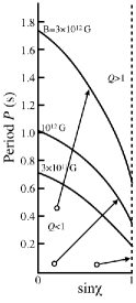
Figure 19: Pulsar extinction line in a $P-\sin\chi$ diagram for different magnetic fields. Arrows show the evolution tracks of individual pulsars in the model of the current losses (29)–(30) (Beskin et al., 1993).

The average inclination angle $\langle\chi\rangle_{\tau_{\rm D}}$ for a given range of ages $\tau_{\rm D}$ can decrease, even if the inclination angles of individual pulsars increases with time, in accord with Eqn. (32). This is a consequence of the dependence of the magnetospheric charge density on the inclination angle $\chi$. For example, in the picture of Ruderman & Sutherland (1975), radio emission results from a secondary electron-position cascade, initiated by pair-production from curvature-radiation photons. The acceleration of primary electrons within a gap produced these curvature photons. The Goldreich-Julian charge density $\rho_{\rm GJ}\approx\Omega B\cos\chi/(2\pi c)$ sets the accelerating potential across the gap. As a pulsar ages, $\rho_{GJ}$ and the accelerating potential decline with $\Omega$. The area of the polar cap also decreases as fewer field lines penetrate the light cylinder, and those remaining within the polar cap are less curved. As Eqn. (4) shows, the mean free path to pair production increases; the gap becomes wider. When the gap width is comparable to the polar-cap radius, the cascade, and radio emission, terminate.

Because the charge density depends on $\cos\chi$ as well as $B_{0}$ and $\Omega$, death comes to pulsars with different inclinations, but the same magnetic field, at different spin periods $P$. Evaluation of the Ruderman & Sutherland model yields $P_{max}\propto B_{0}^{8/9}(\cos\chi)^{2/3}$. Indeed, as can be seen from Figure 19, for given values of the pulsar period $P$ and the magnetic field $B_{0}$, the production of particles is suppressed precisely at inclinations $\chi$ close to $\pi/2$, where the magnetic dipole is nearly orthogonal. Therefore, neutron stars above and to the right of the extinction lines in Figure 19 do not appear as radio pulsars.

Because of this dependence of the pulsar extinction line on $\chi$, the average inclination angles of the observed populations can decrease as the dynamic age increases. A detailed analysis, carried out in Beskin et al. (1984) (see also Beskin & Nokhrina (2004); Beskin & Eliseeva (2005)) on the basis of a kinetic equation describing the distribution of pulsars confirms this picture quantitatively.

Clearly, in any case, that the inclination angle $\chi$ is a key hidden parameter: without taking it into account, it is impossible to construct a consistent theory of the evolution of radio pulsars. Eliseeva et al. (2006) include this possibility in their work, suggesting a possible direction for further improvements in models for the evolution of neutron stars (Lipunov et al., 1996; Story et al., 2007; Popov & Prokhorov, 2007; Gullón et al., 2014).

9 Summary

Pulsars provide elegant, although not simple, laboratories for fundamental electromagnetic processes at high energies. The basic picture of their structures, involving strong magnetic fields and rapid rotation, generation of electron-positron pairs and an energetic wind that carries away the rotational kinetic energy of the pulsar, became clear not long after their discovery a half-century ago. Recent work has begun to uncover the detailed structures of their magnetospheres; the location, size, and optics of their radio emission regions; and evolution of their spins. Some important questions not far from solution include the effect of plasma on the magnetosphere and the possible existence of multiple states; conversion of Poynting flux to a particle wind (the $\sigma$-problem); the location, size, and properties of emission of different pulse components; and whether rotation and magnetic axes tend to co-align or mis-align with time. Further insightful theory, careful statistical studies and targeted observations will lead to deeper understanding, as pulsars continue their role as the archetypal observable neutron stars.