Changing anyonic ground degeneracy with engineered gauge fields

Abstract

For systems of lattice anyons like Majorana and parafermions, the unconventional quantum statistics determines a set of global symmetries (e.g., fermion parity for Majoranas) admitting no relevant perturbations. Any operator that breaks these symmetries explicitly would violate locality if added to the the Hamiltonian. As a consequence, the associated quasi-degeneracy of topologically non-trivial phases is protected, at least partially, by locality via the symmetries singled out by quantum statistics. We show that it is possible to bypass this type of protection by way of specifically engineered gauge fields, in order to modify the topological structure of the edge of the system without destroying the topological order completely. To illustrate our ideas in a concrete setting, we focus on the ${\mathds{Z}}_{6}$ parafermion chain. Starting in the topological phase of the chain (sixfold ground degeneracy), we show that a gauge field with restricted dynamics acts as a relevant perturbation, driving a transition to a phase with threefold degeneracy and ${\mathds{Z}}_{3}$ parafermion edge modes. The transition from the ${\mathds{Z}}_{3}$ to the topologically trivial phase occurs on a critical line in the three-state Potts universality class. Hence, to all effects and purposes, the gauged ${\mathds{Z}}_{6}$ chain realizes the ${\mathds{Z}}_{3}$ parafermion chain. We also investigate numerically the emergence of Majorana edge modes when the ${\mathds{Z}}_{6}$ chain is coupled to a differently restricted gauge field.

I Introduction

The pursuit of topological quantum information processing with mesoscopic arraysterhal2012 ; nussinov2012 ; vijai:15 of Majorana chainskitaev2001 is grounded on well investigated solid state technologies and showcases a new bridge between condensed matter physics and engineering. With current experimental techniques, naturally available topological quantum matter is ill suited for quantum information processing.willett2013 Hence, one should try to design synthetic topological quantum matter with enhanced desirable characteristics. Mesoscopic physics naturally sets the stage for this proposal because the microscopic understanding of interacting topological quantum matter is incomplete. Hence one would like to exploit naturally occurring topological states, not as they come but as building blocks in mesoscopic arrays.

The Majorana chain itself for example is not naturally available, and so the proposals for its realizationalicea12 ; beenakker13 are good examples of the quest for synthetic topological quantum matter. The parafermion chainfendley2012 is an even more ambitious proposal along these lines,alicea15 motivated by a problem that parafermions cannot, at least directly,mong2014 wholly resolve in the end: the limited computational power of Majoranas. With parafermions the ideaclarke2013 ; lindner2012 is to modify mesoscopically the edge of a fractional quantum spin Hall insulator by placing alternating s-wave superconducting and ferromagnetic islands in order to obtain, at low energies, an effective 1d lattice system of hybridized parafermion zero-energy modes. This basic mesoscopic blueprint has excited theoretical interest in various types of parafermion chains, with varying degrees of exoticism in their quantum phase diagramsvaezi13 ; milsted2014 ; zhuang15 ; li15 and also varying potential for mesoscopic realization.milsted2014

Parafermions, and in particular Majoranas, are examples of topological zero-modes. Such modes are good for quantum information processing for three basic reasons: they are local, isolated in energy, and stable. As a consequence, the manifold of ground states of the system that hosts these modes inherits desirable properties. First, its degeneracy is stable. Second, it is possible to perform rotations in the ground manifold by coupling local probes to the topological modes. And third, there is an energy gap to non-topological excitations that sets the time scale for these manipulations.

In spite of their crucial practical value, the stability of topological zero-energy modes poses a problem for incremental design. Take for example the basic blueprint for parafermions of the previous paragraph. The quantum statistics of the emergent lattice parafermion field is characterized by an integer $p\geq 2$, and on the mesoscopic setups of Refs. clarke2013, ; lindner2012, for example, $p$ can only take the values $p=2m$, with $m$ an odd, positive integer. As a consequence, topological qutrits (corresponding to $p=3$) are not included in this otherwise very attractive proposal. This is a problem for the circuit model assisted by topological information processing, since quantum algorithms with qutrits are the best studied ones after qubits. Now, since the ground degeneracy of the $p=6$ parafermion chain is six, it is natural to seek for a design that modifies the basic platform minimally, just enough to halve the degeneracy. But the degeneracy is protected by the stability of the topological zero-energy modes! It should be clear from this example how, in general, incremental design principles can be at odds with “topological” ones.

In this paper, we will propose a method based on symmetry manipulation without symmetry breaking to modify in a controlled fashion the structure of the set of zero-energy modes at the edge of topological quantum matter. Our method in a nutshell starts by identifying discrete gauge fields naturally present in mesoscopic setups and naturally coupled to protecting symmetries. After providing dynamics to the gauge field, some or all of the topological degeneracy disappears. However, if the gauge fluctuations are properly manipulated, it is possible to remove only some of the topological degeneracy. As a consequence, the topological structure of the edge changes in a controlled and predictable way: some zero-modes disappear and the remaining ones control the new ground manifold of the system.

Given the symmetry analysis underlying our idea, one may ask why not just break explicitly the symmetry in question. An explicit symmetry breaking term would in general obtain the same result as that obtained by the gauge field without breaking the symmetry, and, in one space dimension, these two scenarios are often connected by a duality transformation. The answer is rooted deeply in the structure of anyon fields. As we will show, due to anyon statistics, the symmetries that must be manipulated in our framework cannot be explicitly broken without violating locality. Effectively, this observation provides a symmetry-based explanation of the stability, or “protection,” of the zero-energy modes. By coupling the symmetry to a gauge field rather than breaking it, we manage to modify topological zero modes without breaking locality. This idea evolved from our investigation of the effect of phase slips on the Majorana chain,vanHeck2014 since they obtain a ${\mathds{Z}}_{2}$ gauge field minimally coupled to the Majorana degrees of freedom.

The outline of the paper is as follows. In Sec. II, we explain our general ideas using a familiar example, the Majorana chain of Kitaev. The key point is that a ${\mathds{Z}}_{2}$ gauge field arise naturally in physical realizations of topological chains in terms of charged fermions. Making this local $\mathds{Z}_{2}$ gauge field dynamic by mesoscopic manipulation allows to modify the topological edge structure without explicitly breaking fermion-parity. In the following sections, we generalize these ideas to the parafermion chain. In Sec. III, we recall the basic theory of parafermions, discuss the parafermionic generalization of the Majorana chain and show that the global symmetry protecting the parafermionic zero-modes cannot be broken explicitly without violating locality. In Sec. IV, we introduce the gauged parafermion chain where parafermions of degree $p$ are naturally coupled to a $\mathds{Z}_{p}$ gauge field. By means of an exact duality transformation we show that by restricting the dynamics of the ${\mathds{Z}}_{p}$ gauge field to a nontrivial subgroup of $\mathds{Z}_{p}$ we can obtain parafermions of reduced degree without explicitly breaking the protecting symmetry. We show evidence that our construction works as predicted by investigating the period of the supercurrent in a gauged parafermion ring junction as a function of the strength of the gauge fluctuations. Restricting the gauge field dynamics to a $\mathds{Z}_{2}$ subgroup, we obtain a supercurrent periodicity consistent with $\mathds{Z}_{3}$ parafermionic edge modes. In Section V, we confirm in another way that we have $\mathds{Z}_{3}$ parafermionic zero modes in this gauged ${\mathds{Z}}_{6}$ chain by investigating the phase diagram of the system with the DRMG algorithm. The critical exponents of the transition between the topologically non-trivial and trivial phase correspond to the universality class of the three-state Potts model for any finite strength of restricted gauge fluctuations, that is, on a critical line. We also compute the phase diagram of the model with effective $\mathds{Z}_{2}$ parafermionic zero modes (Majoranas). In both cases, the modified topological zero modes are stable and exist in an extended region of coupling space. We conclude with a summary and outlook in Sec. VI.

II Destroying the edge modes of the Kitaev model with gauge fields

In this section we briefly recall the gauged Majorana chaincobanera_holo ; vanHeck2014 in order to keep a concrete example in mind as we proceed to investigate the more complex case of parafermions.

Let us introduce two Hermitian Majorana operators $a_{j}$, $b_{j}$ per site site $j=1,\dots,L$ of a chain, such that

$$\{a_{i},b_{j}\}=0,\quad\{a_{i},a_{j}\}=\{b_{i},b_{j}\}=2\delta_{ij}.$$

Majoranas are related to Pauli matrices,

$$a_{i}=\sigma^{x}_{i}\prod_{j=1}^{i-1}\sigma^{z}_{j},\quad b_{i}=\sigma^{y}_{i}\prod_{j=1}^{i-1}\sigma^{z}_{j},$$ (1)

and fermionic creation and annihilation operators,

$$a_{i} = c_{i}+c_{i}^{\dagger},$$ (2)

$$-{\sf i}b_{i} = -c_{i}+c_{i}^{\dagger}=c_{i}(-1)^{n_{i}}+c_{i}^{\dagger}.$$ (3)

Let $\hat{F}=\sum_{i=1}^{L}n_{i}$ denote the total fermion number operator. Then the operator of fermionic parity

$$(-1)^{\hat{F}}=\prod_{i=1}^{L}(-{\sf i}a_{i}b_{i})$$ (4)

measures the total number of fermions modulo two.

The Majorana chain of Kitaev kitaev2001 is specified by the Hamiltonian

$$H_{\sf k}=-{\sf i}h\sum_{i=1}^{L}a_{i}b_{i}-{\sf i}J\sum_{j=1}^{L-1}b_{j}a_{j+1},$$ (5)

describing the competition between a topologically non-trivial phase for $|h/J|<1$ and a trivial phase for the complementary regime. The points $|h/J|=1$ are critical. In its topologically non-trivial phase, the Majorana chain displays twofold quasi-degeneracy protected by fermionic parity $(-1)^{\hat{F}}$. This symmetry cannot be broken explicitly due to a superselection rule enforcing vanishing matrix elements between sectors distinguished by fermionic parity. Such a superselection rule can be traced back to the requirement of locality of the physical Hamiltonian.

It has been shown in Ref. bravyi:10, that the quasi-degeneracy of the topologically non-trivial phase cannot be lifted by local perturbations. This result suggests that there is no way of modifying the topological structure of the edge by local perturbations. But this inference is in fact incorrect for a physical realization, as opposed to the ideal representation, of the Majorana chain.vanHeck2014 The reason is that the Majorana chain will typically be realized in terms of electrically charged fermions, e.g., electrons, which carry the electromagnetic $U(1)$ gauge structure. Induced superconductivity breaks most of that symmetry, but a $\mathds{Z}_{2}$ part survives.reznik89 This residual gauge symmetry, corresponding to an invariance of energy levels under a local multiplication of the Majorana operators $a_{j}$, $b_{j}$ by a factor of $-1$, is no longer manifest in the Majorana chain due to a tacit but specific gauge choice. Restoring the gauge fields normally used to absorb the effects of these residual gauge transformations leads to the Hamiltonian

$$H_{\sf gk}=-{\sf i}h\sum_{i=1}^{L}a_{i}b_{i}-\sum_{j=1}^{L-1}\bigl{[}{\sf i}Jb_{j}a_{j+1}\tau_{j}^{z}+\kappa\tau_{j}^{x}\bigr{]}.$$ (6)

of the gauged Majorana chaincobanera_holo ; vanHeck2014 The ${\mathds{Z}}_{2}$ gauge field is represented by Pauli matrices $\tau_{j}^{x}$, $\tau_{j}^{z}$, placed on the links $j=1,\dots,L-1$ of the chain. For $\kappa\neq 0$, the gauge field is quantum dynamic.footnote2

The gauged Majorana chain must be supplemented with gauge constraints identifying physical states. Since the $U(1)$ symmetry originates from electromagnetism, all physical states should obey the $\mathds{Z}_{2}$ descendant of Gauss law. The chain has local symmetries

$$G_{1} =(-{\sf i}a_{1}b_{1})\tau_{1}^{x},\quad G_{L}=\tau^{x}_{L-1}(-{\sf i}a_{L}b_{L}),$$ (7)

$$G_{j} =\tau_{j-1}^{x}(-{\sf i}a_{j}b_{j})\tau_{j}^{x}\quad(j=2,\dots,L-1),$$ (8)

and enforcing the Gauss law corresponds to demanding that the local symmetries $G_{j}$ for $j=2,\dots,L$ of the gauged Majorana chain act as the identity on physical states, $G_{j}=\mathds{1}$.fradkin

The perturbation proportional to $h$ in Eq. (6) plays a subtle but definite role in tying the fate of the topologically non-trivial phase to the gauge field. The reason may be traced back to the effect of the gauge field on the topological boundary modes of the Majorana chain. For $h=0$, the gauged Majorana chain displays exact zero-energy modes

$$[H_{\sf gk}|_{h=0},a_{1}]=0=[H_{\sf gk}|_{h=0},b_{L}],$$ (9)

perfectly localized at the end points of the chain and completely insensitive to the gauge field. This insensitivity disappears as soon as $h\neq 0$. In the absence of gauge fluctuations, $\kappa=0$, it is still possible to compute explicitly the evolution of the edge modes with $h$. We obtain

$$\gamma_{l} = a_{1}+\sum_{i=2}^{L}\Big{(}\frac{h}{J}\Big{)}^{i-1}a_{i}\tau^{x}_{i-1}\dots\tau_{1}^{x},$$ (10)

$$\gamma_{r} = b_{L}+\sum_{i=1}^{L-1}\Big{(}\frac{h}{J}\Big{)}^{L-i}b_{i}\tau^{x}_{i}\dots\tau^{x}_{L-1},$$ (11)

with

$${}[H_{\sf gk}|_{\kappa=0},\gamma_{l}] = 2{\sf i}J\Big{(}\frac{h}{J}\Big{)}^{L}b_{L}\tau^{x}_{L-1}\dots\tau^{x}_{1},\quad$$ (12)

$${}[H_{\sf gk}|_{\kappa=0},\gamma_{r}] = -2{\sf i}J\Big{(}\frac{h}{J}\Big{)}^{L}a_{1}\tau^{x}_{1}\dots\tau^{x}_{L-1}.$$ (13)

The gauge field and Majorana (quasi) zero-energy boundary modes are now explicitly intertwined. In general, any gauge invariant perturbation, no matter how small, will suffice to intertwine the topological zero modes with the gauge field.

For some physical setups, due to the stiffness of the phase of the superconducting condensate, the dynamics of the gauge field is strongly suppressed, $\kappa\approx 0$. In this case, the gauge fields may be removed from the theory by a specific gauge choice in order to recover the topologically non-trivial Majorana chain (5). However, we have showed in a previous publicationvanHeck2014 that a finite value for $\kappa$ may be obtained through quantum phase slips in a mesoscopic implementation of the Kitaev model. At finite $\kappa$, the properties of the Kitaev model are fundamentally altered, because $\kappa$ measures the strength of a relevant perturbation of fermionic parity. Any non-zero value of $\kappa$ will remove the topological degeneracy of the Majorana chain for large enough system size. But why is this the case?

One explanation comes from solving the gauge constraints (7) for $\tau_{j}^{x}$, giving

$$\tau_{j}^{x}=\prod_{k=1}^{j}(-{\sf i}a_{k}b_{k})=(-1)^{\hat{F}}\prod_{k=j+1}^{L}(-{\sf i}a_{k}b_{k}).$$ (14)

In this way the dynamics of the gauge field $\tau_{j}^{z}$ drives nonlocal parity measurement of the part of the chain to the left and to the right of site $j$, which is, in general, incompatible with the topological degeneracy. While the gauge fields are local degrees of freedom, they have highly nonlocal effects on the electronic degrees of freedom, which makes them prime candidates for the manipulation of topological phases without breaking protecting symmetries. Moreover, the effects we are describing are not tied to the mean field approximation. Very recently there has been some progress in the investigation of particle number conserving Majorana chains,ortiz14 ; iemini15 and, as should be clear from our arguments, we would not expect our conclusions to be any different for the ${\mathds{Z}}_{2}$ gauged versions of such models.

To summarize, discrete gauge theories can emerge in a natural, controllable way in physical realizations of topological zero-energy boundary modes. Moreover, for the Majorana chain, one can destroy the topologically non-trivial phase phase by gauging the global symmetry of fermionic parity and making the corresponding $\mathds{Z}_{2}$ gauge field dynamic. For parafermions, a richer structure is possible. This is the subject of the rest of the paper.

III Protection of the edge modes of the parafermion chain by locality

In this section we will briefly recall the basics of parafermions in one dimension, introduce the parafermion chain as a natural generalization of the Majorana chain, and explain how the ground degeneracy of the parafermion chain is protected by the interplay between locality and anyonic statistics. There is a very recent review on parafermions Ref. alicea15, that the reader may consult for further details on implementation proposals.

Parafermions are described in terms of a natural generalization of the Majorana operators of the previous section. A one-dimensional, lattice-regularized parafermion field, defined on sites $i=1,\dots,L$, has the following properties alcaraz1981

$$\Gamma_{i}\Delta_{j} = \omega\Delta_{j}\Gamma_{i}\quad(i\leq j),$$ (15)

$$\Gamma_{i}\Gamma_{j} = \omega\Gamma_{j}\Gamma_{i}\quad(i<j),$$ (16)

$$\Delta_{i}\Delta_{j} = \omega\Delta_{j}\Delta_{i}\quad(i<j),$$ (17)

$$\Gamma_{i}^{p}= \mathds{1} =(-1)^{p-1}\Delta_{i}^{p},$$ (18)

where $\omega=e^{i2\pi/p}$ is a $p$-th root of unity. The order $p=2,3,\dots$ of the parafermion field characterizes the exchange (Eqs. (15), (16), and (17)) and exclusion (Eq. (18)) statistics of these degrees of freedom.cobanerafp In addition, the parafermion field is unitary,

$$\Gamma_{i}\Gamma_{i}^{\dagger}=\mathds{1}=\Delta_{i}\Delta_{i}^{\dagger}.$$ (19)

Up to a phase, parafermions of order $p=2$ are Majorana operators. More precisely,

$$\Gamma_{j}=a_{j},\quad\Delta_{j}=-{\sf i}b_{j}\qquad\quad(p=2).$$ (20)

It is in general true of everything that follows that setting $p=2$ will recover some standard facts about fermions.

Following the reasoning for the construction of the Majorana chain by pairing the second parafermion on each site with strength $J$ with the first one the next site, one obtains the parafermion chainfendley2012

$$H_{\sf p}=-\frac{h}{2}\sum_{i=1}^{L}(\Gamma_{i}^{\dagger}\Delta_{i}+H.c.)-\frac{J}{2}\sum_{i=1}^{L-1}(\Delta_{i}\Gamma_{i+1}^{\dagger}+H.c.).\ \ \ \$$ (21)

For $h=0$, the parafermion chain displays exact zero-energy parafermion edge modes,

$$[H_{\sf p},\Gamma_{1}]=0=[H_{\sf p},\Delta_{L}],$$ (22)

perfectly localized on the end points of the chain. As a consequence, the ground energy level is $p$-fold degenerate, and, in fact, every energy level is at least $p$-fold degenerate. This is the topological degeneracy of the parafermion chain. Small values of $h$footnote3 will not remove the topological (quasi-)degeneracy of the ground energy level, but may remove the topological degeneracy of excited energy levels.fendley2012 ; jermyn14

For the Majorana chain there is a strong link between topological degeneracy and fermionic parity. Is there something similar for parafermions? In order to obtain a precise answer to this question it is necessary to relate the parafermion field to a charged field and an underlying Fock space. Let us introduce creation and annihilation operators $C_{i}^{\dagger},C_{i}$ satisfying the relationscobanerafp

$$C_{i}^{\dagger\,p} = 0=C_{i}^{p},$$ (23)

$$C_{i}^{l}C_{i}^{\dagger\,l} + C_{i}^{\dagger\,(p-l)}C_{i}^{p-l}=\mathds{1},$$ (24)

$$C_{i}C_{j} = \omega C_{j}C_{i}\quad(i<j),$$ (25)

$$C_{i}C_{j}^{\dagger} = \bar{\omega}C_{j}^{\dagger}C_{i}\quad(i<j),$$ (26)

($l=1,\dots,p-1$) where the bar denotes complex conjugation, $\bar{\omega}=e^{-i2\pi/p}$. The number operator for these “Fock parafermions” cobanerafp is

$$N_{i}=\sum_{l=1}^{2m-1}C_{i}^{\dagger\,l}C_{i}^{l},$$ (27)

and the Fock vacuum satisfies $C_{i}|0\rangle=0,\ \forall i$. Let $\hat{P}=\sum_{i=1}^{L}N_{i}$ denote the total parafermion number operator. Then

$$\omega^{\hat{P}}=e^{{\sf i}2\pi\hat{P}/p}$$ (28)

measures the parafermionic parity.

The analogy between $\omega^{\hat{P}}$ and $(-1)^{F}$ is compelling, but it is not clear yet whether $\omega^{\hat{P}}$ is a symmetry of the parafermion chain. The relation between Fock and standard parafermions iscobanerafp

$$\Gamma_{i} = C_{i}+C_{i}^{\dagger\,(p-1)},$$ (29)

$$\Delta_{i} = C_{i}\omega^{N}_{i}+C_{i}^{\dagger\,(p-1)}.$$ (30)

It is illuminating to compare Eqs. (2) and (29), and Eqs. (3) and (30). Since $C_{i}^{\dagger\,(p-1)}\omega^{N_{i}}=C_{i}^{\dagger\,(p-1)}$, then

$$\Gamma_{i}^{\dagger}\Delta_{i}=C_{i}^{\dagger}C_{i}\omega^{N_{i}}+C_{i}^{p-1}C_{i}^{\dagger\,(p-1)}=\omega^{N_{i}}.$$ (31)

Hence,

$$\omega^{\hat{P}}=\prod_{i=1}^{L}\Gamma_{i}^{\dagger}\Delta_{i}.$$ (32)

It is straightforward now to check that the parafermionic parity is indeed a symmetry of the parafermion chain.

Similar to the fermionic parity $(-1)^{\hat{F}}$ in the Majorana case, the parafermionic parity $\omega^{\hat{P}}$ distinguishes the various ground states of the parafermion chain. The parafermion field transforms under this symmetry as

$$\bar{\omega}^{\hat{P}}\Gamma_{i}\omega^{\hat{P}}=\omega\Gamma_{i},\quad\bar{\omega}^{\hat{P}}\Delta_{i}\omega^{\hat{P}}=\omega\Delta_{i}.$$ (33)

The stability of the parafermionic zero modes is explained by the fact that $\omega^{\hat{P}}$ is always a symmetry of any local Hamiltonian of parafermions: for these systems, the global ${\mathds{Z}}_{p}$ symmetry $\omega^{\hat{P}}$ cannot be explicitly broken without violating locality.

Why is this so? In order to answer this question, it is useful to introduce an explicit realization of parafermions analogous to the relation between Majoranas and Pauli matrices, Eq. (1). First, associate to each site of the chain a pair of unitary $p\times p$ matrices $U_{i},V_{i}$, often called clock or circulant matrices, that commute on different sites and otherwise satisfy

$$V_{i}U_{i}=\omega U_{i}V_{i},\quad V_{i}^{p}=U_{i}^{p}=\mathds{1}.$$ (34)

We can represent a single pair of clock matrices as

$${U}=\begin{pmatrix}1&0&0&\cdots&0\\ 0&\omega&0&\cdots&0\\ 0&0&\omega^{2}&\cdots&0\\ \vdots&\vdots&\vdots&&\vdots\\ 0&0&0&\cdots&0\\ 0&0&0&\cdots&\omega^{p-1}\\ \end{pmatrix},\quad{V}=\begin{pmatrix}0&1&0&\cdots&0\\ 0&0&1&\cdots&0\\ 0&0&0&\cdots&0\\ \vdots&\vdots&\vdots&&\vdots\\ 0&0&0&\cdots&1\\ 1&0&0&\cdots&0\\ \end{pmatrix},$$ (35)

Then,

$$\Gamma_{i}=V_{i}U_{i-1}\dots U_{1},\quad\Delta_{i}=\Gamma_{i}U_{i}.$$ (36)

In this representation we see explicitly the string responsible for the non-trivial exchange statistics. Now it is possible to show that operators $O_{i}$ localized in a finite region around site $i$, meaning that they are constructible as a product of parafermions in that region, commute for disjoint regions if and only if they are invariant under the symmetry $\omega^{\hat{N}}$ of modular conservation of parafermion number. As a consequence any local Hamiltonian of parafermions is invariant under this symmetry as well: this symmetry cannot be explicitly broken without breaking locality.

Let us point out in closing an interesting relation between Fock parafermions and electron fractionalization. For $p=2m$ with $m$ odd, the Fock parafermion field is literallycobanerafrp the $m$th rood of the electron field. More explicitly, the composite fields $C_{i}^{m},C_{i}^{\dagger\,m}$ satisfy canonical anticommutation relations,

$$\{C_{i}^{m},C_{j}^{m}\}=0,\quad\{C_{i}^{m},C_{j}^{\dagger\,m}\}=\delta_{i,j}.$$ (37)

Tunneling between electronic and parafermionic systems can then be modeled by terms of the form $-\Gamma f^{\dagger}C^{m}+H.c.$, where $f$ is a canonical fermionic annihilation operator. Practical applications of this observation were explored in Ref. cobanerafrp, .

For the mesoscopic setups of Refs. clarke2013, ; lindner2012, , it is indeed the case that the integer $m$ characterizes the fractionalization in the system, since the quasiparticles of the fractional spin Hall insulator in the mesoscopic array carry charge $e/m$. The superconductors on the edge induce pairing, and the relation $p=2m$ is then a reflection of the fact that it takes $2m$ quasiparticles to form a Cooper pair. It is interesting to notice that the $m=1$ is allowed. In this simplest case, there is no fractionalization. The 2d insulator is just a spin Hall insulator, and the parafermion field becomes (up to a phase) a lattice Majorana field. Ref. alicea15, offers an up to date overview of proposals for realizing parafermions in mesoscopic arrays.

IV Changing the edge modes of the parafermion chain with gauge fields

In this section we will show how to selectively remove some of the zero-energy edge modes of the parafermion chain. By analogy to the gauged Majorana chain, the basic idea is to first restore the gauge symmetry of the parafermion chain, and then allow for suitably engineered gauge fluctuations in order to split in energy some gauge sectors and not others. The sectors that remain unsplit support parafermionic topological edge modes of reduced order.

The generalization of the $\mathds{Z}_{2}$ gauge field of the Majorana chain is the $\mathds{Z}_{p}$ gauge field $\tau_{i},\sigma_{i}$ satisfying

$$\tau_{i}^{p}=\sigma_{i}^{p}=\mathds{1},\quad\tau_{i}\sigma_{i}=\omega\sigma_{i}\tau_{i}$$ (38)

and commuting otherwise. This algebra is the same algebra as for the clock matrices $U_{i},V_{i}$ of the previous section, but we use a different notation here for clarity. Then the Hamiltonian of the gauged parafermion chain is

$$H_{\sf gp} = -\frac{h}{2}\sum_{i=1}^{L}(\Gamma_{i}^{\dagger}\Delta_{i}+H.c.)$$

$$- \sum_{i=1}^{L-1}\Big{[}\frac{J}{2}(\Delta_{i}\Gamma_{i+1}^{\dagger}\tau_{i}+H.c.)+\kappa(\sigma_{i}^{a}+H.c.)\Big{]}.$$

In general, the design of the mesoscopic setup meant to realize the parafermion chain provides control over the gauge fluctuations, characterized by $\kappa$ and an integer $a=0,\dots,p-1$. The values $\kappa=0$ and/or $a=0$ correspond to quenched gauge fluctuations, that is, no fluctuations at all. For $a>1$ we say that the gauge fluctuations are restricted. The reason will become clear as we proceed.

The local ${\mathds{Z}}_{p}$ symmetries of the chain are

$$G_{1}=(\Gamma_{1}^{\dagger}\Delta_{1})\sigma_{1}^{\dagger},\quad G_{L}=\sigma_{L-1}(\Gamma_{L}^{\dagger}\Delta_{L}),$$ (40)

$$G_{i}=\sigma_{i-1}(\Gamma_{i}^{\dagger}\Delta_{i})\sigma_{i}^{\dagger}\quad(i=2,\dots,L-1),$$ (41)

They seem a priori independent of the details of the gauge fluctuations, and, being local, they cannot be spontaneously broken.elitzur75 What is then the meaning of the of the integer parameter $a$? The answer is that local gauge fluctuations characterized by $a>1$ generate highly nonlocal measurements of parafermion number modulo $p/a$ which split the ground state multiplet, leaving behind a topological degeneracy of reduced degree. This can be seen by removing explicitly the gauge redundancy and performing a duality transformation, as we will show next. Later in this section we will show that this reduced ground state degeneracy corresponds to topological parafermionic edge modes of reduced degree.

IV.1 Changing topological degeneracy with restricted gauge fluctuations

Let us start by rewriting the gauged parafermion chain in terms of the clock matrices of Eq. (35),

$$H_{\sf gp}= - \frac{h}{2}\sum_{i=1}^{L}(U_{i}+U_{i}^{\dagger})$$

$$- \sum_{i=1}^{L-1}\Big{[}\frac{J}{2}(V_{i}V_{i+1}^{\dagger}\tau_{i}+H.c.)+\frac{\kappa}{2}(\sigma_{i}^{a}+\sigma_{i}^{\dagger\,a})\big{]},$$

by virtue of the transformation Eq. (1). The resulting model is akin to, but not quite the same as a ${\mathds{Z}}_{p}$ Higgs model if $a\neq 1$. In terms of clock matrices, the gauge symmetries are $G_{1}=U_{1}\sigma_{1}^{\dagger}$, $G_{i}=\sigma_{i-1}U_{i}\sigma_{i}^{\dagger}$ for $i=2,\dots,L-1$ and $G_{N}=\sigma_{N-1}U_{N}$. The global symmetry $\omega^{\hat{P}}$ simply reads

$$\omega^{\hat{P}}=\prod_{i=1}^{L}U_{i}.$$ (43)

By introducing simultaneous eigenstates $|\{u_{j}\}\rangle$ of the clock matrices $U_{j}$,

$$U_{j}|\{u_{j}\}\rangle=\omega^{u_{j}}|\{u_{j}\}\rangle\quad(j=1,\dots,L),$$ (44)

and simultaneous eigenstates $|\{\sigma_{j}\}\rangle$ of the clock matrices $\sigma_{j}$,

$$\sigma_{j}|\{\sigma_{j}\}\rangle=\omega^{\sigma_{j}}|\{\sigma_{j}\}\rangle\quad(j=1,\dots,L-1)$$ (45)

we can define gauge-fixed states on the tensor-product space of the matter and gauge fields. They are of the form

$$|\{u_{j}\}\rangle_{\text{gf}}=|\{u_{j}\}\rangle\otimes|\{\sigma_{j}=\sum_{i>j}(\alpha_{i}-u_{i})\}\rangle,$$ (46)

with integers $\alpha_{i}$ defined for $i=2,\dots,L$. The states belonging to the gauge sector labeled by the $\alpha_{i}$ obey the relation

$$G_{i}|\{u_{j}\}\rangle_{\text{gf}} =\omega^{\alpha_{i}}|\{u_{j}\}\rangle_{\text{gf}}\quad(i=2,\dots,L),$$ (47)

and the physical sector corresponds to the choice $\alpha_{i}=0$. Projecting the Hamiltonian onto the gauge-fixed states leads to the gauge-fixed Hamiltonian

$$H_{\sf{gp}}^{\text{gf}}= - \frac{h}{2}\sum_{i=1}^{L}(U_{i}+U_{i}^{\dagger})$$

$$- \sum_{i=1}^{L-1}\Big{[}\frac{J}{2}V_{i}V_{i+1}^{\dagger}+\frac{\kappa}{2}\prod_{j>i}(\omega^{a\alpha_{j}}U_{j}^{\dagger a})+H.c.\Big{]},$$

where the operator $U_{i}$ acts in the natural way on the gauge-fixed states,

$$U_{j}|\{u_{j}\}\rangle_{\text{gf}}=\omega^{u_{j}}|\{u_{j}\}\rangle_{\text{gf}}.$$ (49)

For $\kappa=0$, the gauge-fixed parafermion chain $H_{\sf{gp}}^{\text{gf}}$ is just the celebrated clock model (see Ref. ortiz:12, for an up-to-date review), and one could translate back to parafermions to recover the standard parafermion chain. But for $\kappa\neq 0$, the gauge-fixed Hamiltonian shows explicitly how local gauge fluctuations at finite $\kappa$ affect the parafermionic degrees of freedom in a highly nonlocal way. The strings in $H_{\sf{gp}}^{\text{gf}}$ are not local neither in terms of clock or parafermion degrees of freedom. On the parafermions, they correspond to nonlocal measurements of parafermion number modulo $p/a$.

To see why this corresponds to a reduction of the ground state degeneracy, we note that the gauge-fixed Hamiltonian may be brought into a local form by means of the duality transformation

$$V_{i} \mapsto\prod_{j=1}^{i}U_{j}\quad(i=1,\dots,L),$$

$$U_{i} \mapsto V_{i}^{\dagger}V_{i+1}\quad(i=1,\dots,L-1),$$ (50)

$$U_{L} \mapsto V_{L}^{\dagger},$$

exact for finite chains.ortiz:12 The resulting Hamiltonian is

$$H_{\sf gp}^{\text{gf},D}= -\frac{h}{2}(V_{L}^{\dagger}+H.c.)-\frac{h}{2}\sum_{i=1}^{L-1}(V_{i}^{\dagger}V_{i+1}+H.c.)$$ (51)

$$-\sum_{i=1}^{L-1}\Big{[}\frac{J}{2}U_{i+1}^{\dagger}+\frac{\kappa}{2}V_{i+1}^{a}\,\prod_{j>i}\omega^{a\alpha_{j}}+H.c.\Big{]}$$

and the global symmetry $\omega^{\hat{P}}$ is mapped onto a boundary symmetry, $\omega^{\hat{P}}\mapsto V_{1}^{\dagger}$.

The Hamiltonian $H_{\sf gp}^{\text{gf},D}$ makes the role of the gauge fluctuations particularly clear. Let us focus on the physical sector $(\alpha_{i}=0$) for simplicity. Then, if we neglect finite-size corrections, that is, the boundary term $hV_{L}/2+H.c.$, $H_{\sf gp}^{\text{gf},D}$ takes the simpler form $\sum_{i}H_{i}$, with

$$H_{i}=-\Big{[}\frac{J}{2}U_{i+1}^{\dagger}+\frac{\kappa}{2}V_{i+1}^{a}+\frac{h}{2}V_{i}^{\dagger}V_{i+1}\Big{]}+H.c.$$ (52)

Let $a/p=a^{\prime}/r$, with $a^{\prime}$ and $r$ relative primes, and suppose for simplicity that $p=rs$ with $r$ and $s$ also relative primes. Then, the equivalent $\omega^{\hat{P}_{D}}$ of Eq. (43) with the matrices $U_{i}$ of the dual model (51), gives

$$\bar{\omega}^{r\hat{P}_{D}}V_{i}^{a}\omega^{r\hat{P}_{D}}=V_{i}^{a},$$ (53)

since $e^{{\sf i}2\pi ar/p}=1$. Hence, the “longitudinal field” $\kappa$ breaks the symmetry $\omega^{\hat{P}_{D}}$, but not completely if $a>1$: The ${\mathds{Z}}_{s}$ symmetry $\omega^{r\hat{P}_{D}}$ survives the gauge fluctuations unscathed. Conversely, the ${\mathds{Z}}_{r}$ symmetry $\omega^{s\hat{P}_{D}}$ is completely broken. In this way, gauge fluctuations obtain specific relevant perturbations that reduce but do not remove completely the topological degeneracy of the parafermion chain.

IV.2 Effect of restricted gauge fluctuation on topological boundary modes

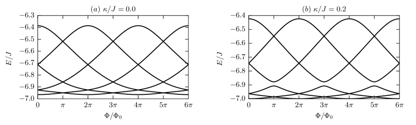
Figure 1: Lowest energy levels of the Hamiltonian (62) modeling a $\mathds{Z}_{6}$ parafermionic ring chain as a function of the enclosed flux $\Phi$. The $\mathds{Z}_{6}$ parafermions are coupled to $\mathds{Z}_{6}$ gauge fields whose dynamics is restricted to $\mathds{Z}_{2}$. ($a$) For static gauge fields with $\kappa=0$, the spectrum shows the $12\pi$ flux periodicity expected for $\mathds{Z}_{6}$ parafermions. ($b$) For dynamic gauge fields with $\kappa=0.2J$, the flux periodicity is reduced from $12\pi$ to a flux periodicity of $6\pi$ consistent with effective $\mathds{Z}_{3}$ parafermions.

Restricted gauge fluctuations obtain a bulk relevant perturbation that partially removes the topological degeneracy of the parafermion chain. What is the effect on the edge modes? Here we address this question in terms of the Josephson effect, generalizing the celebrated anomalous periodicity of the supercurrent in the Majorana chain for investigating gauged Parafermion chains.

Let us take $p>a=s>1$ for concreteness, so that $a/p=1/r$, with $r$ and $s$ relative primes. Then the exact zero modes

$$\tilde{\Gamma}_{1}=\Gamma_{1}^{r},\quad\tilde{\Delta}_{L}=\Delta_{L}^{r}$$ (54)

of the gauged Parafermion chain with $h=0$ realize parafermions of reduced degree $s$. These topological modes commute with the symmetry $\omega^{s\hat{P}}$ that is effectively, but not explicitly, broken by the restricted gauge fluctuations. Hence, we expect these zero modes to survive the gauge fluctuations because they live in sectors of constant $\omega^{s\hat{P}}$ and will not become split in energy.

We can make this picture quantitative and very close to the situation for the gauged Majorana chain if we recall a technical result about clock matrices. Let us write $\tau_{i}^{(q)},\sigma^{(q)}_{i}$ for the clock matrices of order $q=r,s$. Then we have the identificationscobanerafp

$$\sigma_{i}\cong\sigma^{(r)}_{i}\otimes\sigma^{(s)}_{i},\quad\tau_{i}\cong(\tau^{(r)}_{i})^{n}\otimes(\tau^{(s)}_{i})^{n},$$ (55)

with $n$ the unique solution offootnote4

$$(r+s)n=1\ \ (\mbox{mod}\ p).$$ (56)

In particular,

$$\sigma_{i}^{s}\cong(\sigma^{(r)}_{i})^{s}\otimes\mathds{1}^{(s)}_{i}.$$ (57)

Sincefootnote5

$$(\tau^{(r)}_{i})^{n}(\sigma^{(r)}_{i})^{s}=e^{{\sf i}2\pi/r}(\tau^{(r)}_{i})^{n}(\sigma^{(r)}_{i})^{s},$$ (58)

we can make the simpler identification

$$\sigma_{i}^{s}\cong\sigma^{(r)}_{i}\otimes\mathds{1}^{(s)}_{i},\quad\tau_{i}\cong\tau^{(r)}_{i}\otimes\tau^{(s)}_{i}.$$ (59)

In terms of the identification of Eq. (59), we can rewrite the gauged Parafermion chain in reduced form,

$$H_{\sf gp}^{\prime}= - \frac{h}{2}\sum_{i=1}^{L}(\Gamma_{i}^{\dagger}\Delta_{i}+H.c.)$$

$$- \sum_{i=1}^{L-1}[\frac{J}{2}(\alpha_{i}\Delta_{i}\Gamma_{i+1}^{\dagger}\tau^{(r)}_{i}+H.c.)+\kappa(\sigma^{(r)}_{i}+H.c.)].$$

The site-dependent numerical phases $\alpha_{i}$ are $s$ roots of unity obtained from diagonalizing the $\tau^{(s)}_{i}$. Since, in particular, $\alpha_{i}^{p}=1$, they can be removed by a gauge choice in the definition of the parafermion field. Hence the situation is as follows: A parafermion chain coupled to a ${\mathds{Z}}_{p}$ gauge field with restricted fluctuations ($a=s=p/r$) is equivalent to a parafermion chain coupled to a ${\mathds{Z}}_{r}$ gauge field with unrestricted gauge fluctuations ($a=1$). Based on our experience with the gauged Majorana chain, we expect that the ${\mathds{Z}}_{r}$ topological boundary modes

$$\tilde{\tilde{\Delta}}_{1}=\Delta_{1}^{s},\quad\tilde{\tilde{\Delta}}_{L}=\Delta_{L}^{s}$$ (61)

will be gapped out by the ${\mathds{Z}}_{r}$ gauge field, leaving behind the ${\mathds{Z}}_{s}$ zero modes of Eq. (54).

We can check this claim explicitly by extending the theory of the $4\pi$ Josephson effect in the Majorana chain to our gauged parafermion chain, or more precisely, to $\tilde{H}_{\sf pg}$ to avoid unnecessary numerical cost. To drive a supercurrent across the gauged parafermion chain it is convenient to close the system into a ring threaded by a flux $\Phi$. The Hamiltonian for this parafermion ring junction is

$$H^{\prime}(\Phi)=H_{\sf gp}^{\prime}-\frac{J}{2}(C_{L}^{\dagger}\tau^{(r)}_{L}C_{1}e^{-{\sf i}2\Phi/p}+H.c.)$$ (62)

(the Fock parafermions $C_{i}$, $C_{i}^{\dagger}$ of charge $2e/p$ were introduced in the previous section). The tunneling term is also coupled to the gauge field in order to preserve gauge invariance. The gauge symmetries of the ring junction are

$$G_{i}^{\prime}=\sigma^{(r)}_{i-1}(\Gamma_{i}^{\dagger}\Delta_{i})(\sigma^{(r)}_{i})^{\dagger}\quad(i=i+L).$$ (63)

Let us consider for concreteness a ${\mathds{Z}}_{2}$ gauge field coupled to parafermions of order $p=6$, so that $r=2$ and $s=3$. Fig. 1($a$) shows the six lowest energy levels of $H_{\sf gp}(\Phi)$ in the ${\mathds{Z}}_{2}$ gauge invariant sector and for $\kappa=0=h$. Any gauge sector would show the same result since they are all degenerate in energy. The full $12\pi$ Josephson effect expected of the usual $p=6$ parafermion chainclarke2013 ; cobanerafp is clearly visible. For $\kappa/J=0.2$ and $h=0$, the period of the supercurrent has decreased to $6\pi$, c.f. Fig. 1($b$). The zero modes responsible for this periodicity are precisely the parafermionic zero modes $\tilde{\Gamma}_{1},\tilde{\Delta}_{L}$ of order $s=3$.

We will show in Sec. V that the term proportional to $\kappa$ is a relevant perturbation. As the system size increases, smaller and smaller values of $\kappa$ suffice to produce an appreciable change in the periodicity of the supercurrent.

V Stability against local perturbations at zero temperature

As we saw in the previous section, gauge fluctuations change the topological edge structure of the parafermion chain. What is the stability of the modified edge against a generic perturbation? In order to gain some insight into this problem, in this section we determine numerically the phase diagram of the gauged parafermion chain in the coupling space defined by $h$ and $\kappa$. Recall that the perturbation of strength $h$ favors a trivial pairing of parafermions. For numerical investigations it is convenient to explicitly remove the gauge redundancy of the gauged parafermion chain. Hence in this section we work exclusively with the dual Hamiltonian $H_{\sf gp}^{\text{gf},D}$ of Eq. (51) in the gauge invariant sector.

Since energy levels, and quantum phase diagrams in particular, are insensitive to the distinction between parafermion and clock chains, let us emphasize once more the conceptual issue at stake. The gauged parafermion chain and the clock Hamiltonian of Eq. (IV.1), or its gauge-fixed version, are the same Hamiltonian from an spectral point of view. However, if one were to realize $H_{\sf gp}$ on a physical platform, then the representation Eq. (IV) would be naturally suited for a fermionic platformclarke2013 ; lindner2012 , and that of Eq. (IV.1) a bosonic one, e.g., bosonic cold atoms. However, for the Hamiltonian $H_{\sf gp}$ written as in Eq. (IV.1), it is easy to break some or all of its global symmetries explicitly with perturbations of the form $-h_{s}\sum_{i=1}^{L}(V_{i}^{s}+H.c.)$. No gauge field is needed to effectively generate such terms. Hence, in a cold atom realization, the ground degeneracy of $H_{\sf gp}$ is fragile.nussinov09 In contrast, such perturbations are non-local in terms of parafermions and strictly absent in fermionic realizations, except, effectively, as gauge fields!

In the following, we will focus on parafermions of order $p=6$. Then it is possible to restrict the gauge field dynamics to $\mathds{Z}_{r}$ with $r=2,3$ by taking $a=3,2$ respectively. We call the corresponding models the ${\mathds{Z}}(6,2)$ and ${\mathds{Z}}(6,3)$ chains.

V.1 Critical exponents for $\mathds{Z}(6,2)$

In the previous section, we have discussed that increasing $h$ should eventually drive the system from a topological phase into a trivial phase. If we indeed have $\mathds{Z}_{3}$ parafermionic zero modes for finite $\kappa$, as suggested by the supercurrent numerical calculation of Sec. IV, this must be reflected in the universality class of the transition. To confirm the presence of $\mathds{Z}_{3}$ parafermionic zero modes, we calculate the critical exponents of the transition by means of a detailed finite-size scaling analysis.

For the analysis of the system, we use the Hamiltonian (51) in the physical sector $\alpha_{i}=0$ which decomposes into subspaces $H_{q}$ to eigenvalue $e^{i2\pi q/6}$ of the conserved quantity $V_{1}$. We assume that a single relevant operator associated with $h$ will drive a transition from a symmetry-broken $\mathds{Z}_{3}$ phase into a trivial phase. Consequently, a scaling analysis along the lines of the Ising transition in absence of symmetry-breaking fields (in the bulk) applies.cardy While the bulk terms of $H_{q}$ are invariant under the $\mathds{Z}_{3}$ symmetry, the operator $v_{N}$ and the operator $(e^{-i2\pi q/6}v_{2}+H.c)$ arising from the projection on $H_{q}$ explicitly breaks this symmetry at the boundary. Although negligible in the thermodynamic limit, those symmetry-breaking boundary operators are expected to give rise to irrelevant scaling fields leading to increased finite-size effects. campostrini:14

For the numerical determination of the location of the critical point and the critical exponents, we use the density renormalization group (DMRG) algorithm and variationally determine the eigenstates of the Hamiltonian Eq. (51) in the ground state sector $q=0$, requiring for each variational state $|\psi\rangle$ with (approximate) eigenvalue $\lambda$ a precision of at least $\sqrt{\langle\psi|(H-\lambda I)^{2}|\psi\rangle}/\lambda\leq 10^{-7}$. We analyze systems with system size $N=16,32,64,128$ sites and maximal internal bond dimensions $D=128$.

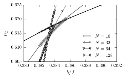
Figure 2: Behavior of the Binder cumulants $U_{L}=1-\langle m^{4}\rangle/3\langle m^{2}\rangle^{2}$, defined in terms of the magnetization $m=\sum_{i=1}^{N}(v_{i}+v_{i}^{\dagger})/2N$, for systems of different sizes $N$ along the line $h=\kappa$ in vicinity of the crossing points.

Let us start with a detailed finite-size scaling analysis along the line $h=\kappa$. The similarity to the Ising case suggests exploiting the Binder cumulant $U_{L}=1-\langle m^{4}\rangle/3\langle m^{2}\rangle^{2}$ of the “magnetization per site” $m=\sum_{i=1}^{N}(v_{i}+v_{i}^{\dagger})/2N$ for a precise determination of the location of the critical point. Considering one irrelevant scaling field with renormalization group eigenvalue $-\omega<0$ and expanding the scaling fields to lowest non-vanishing order, the Binder cumulant satisfies the scaling relationpelissetto:02

$$U_{L}=\Phi\bigl{(}|h-h_{c}|N^{1/\nu},u_{0}N^{-\omega}\bigr{)}.$$ (64)

Here $\Phi$ is a universal scaling function, $\nu$ is the critical exponent associated with the divergence of the correlation length, $h_{c}$ is the critical point, and $u_{0}$ is the value of the irrelevant scaling field at the critical point. As before, $N$ denotes the system size. By expanding $\Phi$ around the critical point $(0,u_{0})$, we find that the crossing points $h_{N_{1},N_{2}}$ of the Binder cumulants of different systems with size $N_{1}$, $N_{2}$ scale as

$$|h_{N_{1},N_{2}}-h_{c}|\propto N_{1}^{-1/\nu-\omega}\frac{1-(N_{2}/N_{1})^{-\omega}}{1-(N_{2}/N_{1})^{-1/\nu}}$$ (65)

and thus converge to the critical point $h_{c}$ as $N_{1}$ goes to infinity for fixed ratios $N_{1}/N_{2}$.

Figure Fig. 2 shows the behavior of the Binder cumulants for different system sizes $N=16,32,64,128$ and $D=128$. We obtain the location of the critical point and the exponent $-1/\nu-\omega$ using a Shanks transformation for the data tuples $(N_{1},N_{2})=(16,32),(32,64),(64,128)$. Since we only have 3 data points available, we estimate the errors by varying $h_{c}$ and observing when the data points $|h_{N_{1},N_{2}}-h_{c}|$ in a double-logarithmic plot deviate visibly from a line, yielding $1/\nu+\omega\approx 1.69$ and $h_{c}=0.38426(5)$. In absence of irrelevant scaling fields, the scaling form Eq. (64) predicts that the values of $U_{L}$ of different system sizes $N$ collapse onto a single curve as a function of $z=(h-h_{c})N^{1/\nu}$. The failure of a data collapse assuming the absence of irrelevant scaling fields, using $1/\nu\approx 1.69$, confirms the non-negligible role of irrelevant scaling fields for the scaling analysis.

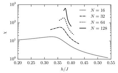
Figure 3: Behavior of the susceptibility $\chi$ along the line $h=\kappa$ for different system sizes $N$. Data points are not indicated for better visual clarity.

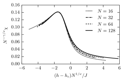
Figure 4: Data collapse of the susceptibility data shown in Fig. 3 with $\nu=0.832$, $\gamma/\nu=1.731$ determined from a minimization of the residuals Eq. (V.1) in an interval of size $\Delta z=\pm 0.4$ around the susceptibility maximum. The critical point $h_{c}$ is fixed at the value obtained using Binder cumulants. Away from the maximum, no complete data collapse is obtained. To the right of the maximum, the curves for different $N$ approach the maximum $N_{\text{max}}=128$ curve monotonously from below, whereas to the left of the maximum, they approach the $N_{\text{max}}$ curve monotonously from above. This systematic structure of the deviations suggests contributions due to irrelevant scaling fields, possibly associated with the symmetry-breaking boundary operators in the Hamiltonian $H_{q}$, as a possible explanation. Data points are not indicated for better visual clarity, the data point spacing is roughly $\Delta z=0.1$ for all curves.

For the determination of the critical exponents $\nu$, $\gamma/\nu$, we consider the susceptibility

$$\chi=N^{2}(\langle m^{2}\rangle-\langle m\rangle^{2}).$$ (66)

In absence of irrelevant scaling fields, $\chi$ satisfies the scaling relation

$$\chi=N^{\gamma/\nu}\tilde{\Phi}\bigl{(}|h-h_{c}|N^{1/\nu}\bigr{)},$$ (67)

where $\tilde{\Phi}$ is a universal scaling function and $\gamma$ is the critical exponent associated with the divergence of the susceptibility at the critical point. The behavior of the susceptibility across the transition is shown in Fig. 3 for different system sizes. According to the scaling form Eq. (67), the susceptibility values $\chi N^{-\gamma/\nu}$ obtained for different system sizes collapse onto a single curve as a function of $z=(h-h_{c})N^{1/\nu}$. Then, for given values of $z$ and $h_{c}$ obtained using Binder cumulants, we extract the critical exponents $\nu$, $\gamma/\nu$ from the susceptibility values by minimizing the quadratic differences

$$\sum_{z}\sum_{i<j}\Bigl{[}\chi_{i}(h_{c}+zN_{i}^{-1/\nu})N_{i}^{-\gamma/\nu}$$

$$-\chi_{j}(h_{c}+zN_{j}^{-1/\nu})N_{j}^{-\gamma/\nu}\Bigr{]}^{2}$$ (68)

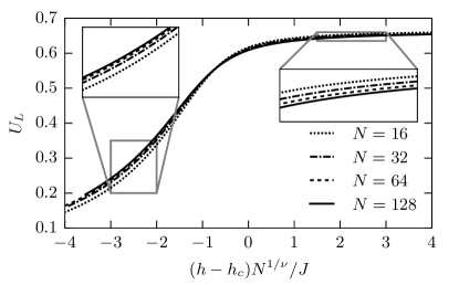
Figure 5: Data collapse of the Binder cumulants $U_{L}$ obtained using $h_{c}$, $\nu$ determined from Binder cumulants and susceptibility. Data points are not indicated for better visual clarity, the data point spacing is roughly $\Delta z=0.1$ for all curves. Insets show close ups of the curves in the marked regions, showing that the distance to the $N_{\text{max}}=128$ curve systematically decreases as $N$ is increased.

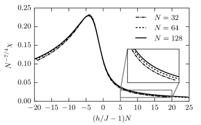
Figure 6: Data collapse of the susceptibility curves obtained for the model (51) along the line $\kappa=0$ with $p=2$ which corresponds to an Ising model with symmetry-breaking boundary conditions, using the exactly known critical point $h_{c}/J=1$ and the critical exponents $\nu=1$, $\gamma=7/4$. The collapse shows a structure similar to the collapse of the susceptibility data obtained along the line $\kappa=h$ for $p=6$ that was shown in Fig. 4, with deviations from perfect data collapse away from the susceptibility peak.

between the rescaled susceptibility curves $\chi_{i}(h)$ of systems of size $N_{i}$. Performing the fit in a range of $\Delta z/J=\pm 0.4$ around the maximum of the scaled susceptibility, which is the most prominent feature, we obtain the data collapse shown in Fig. 4 with $\gamma/\nu=1.731(2)$, $\nu=0.832(3)$.

The error estimates are obtained by checking when data collapses obtained using values $\nu+\Delta\nu$, $\gamma/\nu+\Delta(\gamma/\nu)$ for the critical exponents, with $\nu$, $\gamma/\nu$ as quoted above and $\Delta\nu$, $\Delta(\gamma/\nu)$ some perturbation, show appreciable deviations from the data collapse of Fig. 4. While by choice of the fit region, the collapse shown in Fig. 4 is very good around the maximum, it shows systematic deviations away from it. We note in particular that the distance to the maximal size $N_{\text{max}}=128$ curve is decreasing monotonously as $N$ is increased. Performing the fit around other regions of the susceptibility curve yields data collapses with deviations that do not show a similar internal consistency. A data collapse of the Binder cumulant $Q_{L}$ obtained with $h_{c}$ and $\nu$ as determined above shows reasonable data collapse with deviations showing the same systematic behavior, see Fig. 5.

The systematic behavior of the deviations suggests irrelevant scaling fields due to the symmetry-breaking boundary operators in the Hamiltonian $H_{q}$ as a plausible explanation. In order to show that this explanation is indeed consistent, we have simulated the model (51) with $p=2$ along the line $\kappa=0$, where it is just an Ising model with symmetry-breaking boundary conditions. The collapse of the susceptibility curves of systems with different sizes $N_{i}$, using the exactly known values for the critical point $h_{c}/J=1$ and the critical exponents $\nu=1$, $\gamma=7/4$, is shown in Fig. 6. The data shows good collapse around the susceptibility maximum and deviations away from it, i.e., a structure similar to the collapse discussed previously. This shows that symmetry-breaking boundary operators may indeed be the cause of the irrelevant scaling fields and strongly supports the assumption that our choice of fit region around the susceptibility maximum allows us to extract the critical exponents with a negligible systematic error.

Summing up, we find $\nu=0.832(3)$, $\gamma/\nu=1.731(2)$ for the critical exponents of the transition along the line $h=\kappa$. This result is in good agreement with the exact values $\nu=5/6=0.8\bar{3}$, $\gamma/\nu=26/15=1.7\bar{3}$ expected for the three-state Potts model. wu:82 We thus numerically confirm the transition from a $\mathds{Z}_{3}$ to a trivial phase that was suggested by the structure of the dual Hamiltonian (51) and the periodicity of the supercurrent discussed in Sec. IV.

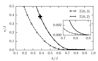
Figure 7: Location of the critical line for the transition from the nontrivial phase (to the left of the line) to the trivial phase (to the right of the line) for the $\mathds{Z}(6,2)$ and $\mathds{Z}(6,3)$ model. The critical line is determined from the crossing points of the Binder cumulants $U_{L}$ for system sizes $(N_{1},N_{2})=(32,64)$ and the Binder cumulants are calculated numerically using the DMRG algorithm with internal bond dimension $D=64$. Data points are marked as small crosses and linearly interpolated for visual guidance. The large cross indicates the position of the point where we have determined the critical exponents $\nu=0.832$, $\gamma/\nu=1.731$ consistent with a $\mathds{Z}_{3}$ phasewu:82 by means of a more detailed finite-size scaling analysis. The inset shows a closeup of the region around $\kappa=0$, showing that in both cases, the critical lines of the models end at the same point at $\kappa=0$.

V.2 Phase diagram

According to our findings for the $\mathds{Z}(6,2)$ model, the crossings of the Binder cumulants indicate the location of the critical point up to small finite-size corrections. In fact, this is expected to hold regardless of whether the $\mathds{Z}_{2}$ subgroup or the $\mathds{Z}_{3}$ subgroup of the gauge fields is dynamic and we will also use Binder cumulants to study the phase boundaries for the $\mathds{Z}(6,3)$ model. In this model, the parafermion edge modes of degree $p=6$ are transmuted into Majorana edge modes.

To determine the phase boundaries of both models, we use the crossings of the Binder cumulants of system sizes $(N_{1},N_{2})=(32,64)$ with internal bond dimension $D=64$. For the $\mathds{Z}(6,2)$ model, we investigated the crossing along lines of constant $\kappa$ for $\kappa/J>0.2$, whereas for $\kappa/J<0.2$, we focused on lines of constant $h$ in order to to ensure that the critical line is hit at approximately right angle. We proceeded similarly for the $\mathds{Z}(6,3)$ model. The resulting phase diagrams of the $\mathds{Z}(6,3)$ and $\mathds{Z}(6,3)$ gauged parafermion chains are shown in Fig. 7. There is a topologically non-trivial $\mathds{Z}_{3}$ phase for the $\mathds{Z}(6,2)$ model and a topologically non-trivial $\mathds{Z}_{2}$ (Majorana) phase for the $\mathds{Z}(6,3)$ model in an extended region of the phase diagram. Notice that the range of $\mathds{Z}_{3}$ criticality in coupling space encompasses a line rather than a point as for the standard ${\mathds{Z}}_{3}$ parafermion chain. This observation may prove useful in connection to a recent blueprint for obtaining Fibonacci anyons;mong2014 we will come back to this point in the outlook.

Finally, let us emphasize that our numerical findings indicate that the two critical lines share a common endpoint marking the end of the critical phase of the ${\mathds{Z}}_{6}$ parafermion chain. Obviously, our results are not totally conclusive due to the limited system sizes and the lack of detailed finite-size extrapolations in that area of the phase diagram. However, we can offer a qualitative explanation of this numerical observation. It is a well-investigated fact that the perturbed, ungauged parafermion chain (a.k.a, the clock model) displays a critical phase for $p>5$, see for example Ref. ortiz:12, for a recent, comprehensive discussion. Imagine now for the sake of the argument that the transition line for the $\mathds{Z}(6,2)$ model were to meet the critical phase of the ${\mathds{Z}}_{6}$ parafermion chain somewhere inside that phase. Then, from that point on, that is, for larger values of $h$, the chain would effectively behave as a ${\mathds{Z}}_{2}$ chain, since the only edge modes left would be the critical Majorana modes. But a ${\mathds{Z}}_{2}$ chain does not support a critical phase. Hence it must be that the critical lines meet at the end of the critical phase. Incidentally, this determines completely the boundary of the critical phase, since the starting point is a function of the final point by self-duality.

VI Summary and Outlook

Topological zero-energy boundary modes are typically stable against generic perturbations, and it is precisely this feature that makes them attractive for quantum information processing. However, it is also this feature that makes them hard to mold in a controlled fashion. Extending our previous work on the effect of phase slips in the Majorana chain of Kitaev, we have argued in this paper that for topological boundary modes associated to a global protecting symmetry, it is possible to modify the topological edge structure in a controlled fashion by engineering a gauge field into the system. The quantum fluctuations of the gauge field act as a relevant perturbation without symmetry breaking, and permit to split the ground degeneracy of the system, partially or completely, depending on the designed properties of the gauge fluctuations. If the gauge field is engineered, by allowing only restricted gauge fluctuations, so that the ground degeneracy is only partially split, then the topological edge modes are modified accordingly, in a controlled and predictable fashion. There is absolutely no risk of driving the system to a trivial phase purely by restricted gauge fluctuations, unless the gauge field is explicitly designed to do so by allowing for unrestricted gauge fluctuations. It would be interesting to recast these results in terms of the group cohomology classification of symmetry protected topological quantum orders and bosonic anomalies.chen13 ; wang15

We have illustrated our ideas with gauged parafermion chains. For generic chains, we performed a symmetry and duality analysis confirming our theoretical predictions. To obtain a more refined picture of the the transmutation of the edge modes and the correlation with critical phenomena, we investigated numerically the ${\mathds{Z}}_{6}$ parafermion chain coupled to a ${\mathds{Z}}_{2}$-like or a ${\mathds{Z}}_{3}$-like gauge field. That is, the dynamics of the physically natural ${\mathds{Z}}_{6}$ gauge field was restricted to achieve a ${\mathds{Z}}_{2}$-like or ${\mathds{Z}}_{3}$-like effect. According to our general picture, the ${\mathds{Z}}_{2}$-like field should transmute the ${\mathds{Z}}_{6}$ edge modes of the parafermion chain into ${\mathds{Z}}_{3}$ edge modes, and we showed numerically that this is the case by computing the period of the supercurrent in a parafermion ring junction as a function of gauge fluctuations. We also obtained the phase diagram of the gauged parafermion chain as a function of gauge fluctuations and a perturbation driving the system to a trivial phase. In this two dimensional phase diagram, the transition between the gauge-driven phase with ${\mathds{Z}}_{3}$ edge modes and the topologically trivial phase occurs on a critical line in the universality class of the ${\mathds{Z}}_{3}$ parafermion chain. From this point of view, the ${\mathds{Z}}_{2}$-gauged ${\mathds{Z}}_{6}$ parafermion chain is indistinguishable from the ungauged ${\mathds{Z}}_{3}$ chain. The general picture is the same for the ${\mathds{Z}}_{3}$-gauged ${\mathds{Z}}_{6}$ parafermion chain. In this case, the edge modes are Majoranas.

Let us mention in closing two potential practical applications of our work. One possibility is to exploit our ideas to create topological qutrits out of ${\mathds{Z}}_{6}$ parafermions. Qutrits have practical advantages over qubits, not because they can provide qualitatively faster algorithms, but because they can polynomialy shorten the length of an algorithm in the circuit model of quantum computation. Of course, the same holds for six-state quantum bits, but here we have face the problem that very little is known about quantum software design with many-leveled logic. Topological qutrits strike a nice balance from this point of view.

Another possibility is to use a gauged ${\mathds{Z}}_{6}$ parafermion chain as a replacement for a ${\mathds{Z}}_{3}$ chain. The ${\mathds{Z}}_{3}$ parafermion chains is one of the key building blocks in a recent blueprintmong2014 for realizing Fibonacci anyons. One difficulty of that blueprint is that, as a building block in this setup, all the chains in a two-dimensional stack must be tuned to their critical point. By contrast, our realization of the ${\mathds{Z}}_{3}$ chain out of the ${\mathds{Z}}_{6}$ chain is critical on a line rather than a point, and the whole line is in the universality class of the ${\mathds{Z}}_{3}$ chain. Moreover, the ${\mathds{Z}}_{6}$ chain is in principle realizable out of the (doubled) $1/3$ fractional quantum Hall state, which is the most stable fractional plateau. We expect that the ${\mathds{Z}}_{2}$ gauge field for this application might also be engineered out of superconducting phase slips, but the situation is not as simple as for the Majorana chain. The mesoscopic details of engineering the required gauge fields will be the subject of an upcoming publication.

- (1) B. Terhal, F. Hassler, and D. DiVincenzo, Phys. Rev. Lett. 108, 260504 (2012).
- (2) Z. Nussinov, G. Ortiz, and E. Cobanera, Phys. Rev. B 86, 085415 (2012).
- (3) S. Vijay, T. H. Hsieh, and L. Fu, arXiv:1504.01724 [cond-mat.mes-hall] (2015).
- (4) A.Y. Kitaev, Phys.-Usp. 44, 131 (2001).
- (5) The experimental attempts to manipulate the quasiparticle excitations of the quantum Hall liquid at filling fraction provide a telling example. See R. L. Willett, Rep. Prog. Phys. 76, 076501 (2013).
- (6) J. Alicea, Rep. Prog. Phys. 75, 076501 (2012).
- (7) C. W. J. Beenakker, Annu. Rev. Con. Mat. Phys. 4, 113 (2013)
- (8) P. Fendley, J. Stat. Mech 11, 11020 (2012).
- (9) J. Alicea and P. Fendley, arXiv:1504.02476 [cond-mat.str-el] (2015).
- (10) R. S. K. Mong et. al., Phys. Rev. X 4, 011036 (2014).
- (11) D. J. Clarke, J. Alicea and K. Shtengel, Nature Commun. 4, 1248 (2013).
- (12) N. H. Lindner, E. Berg, G. Refael, and A. Stern, Phys. Rev. X 2, 041002 (2012).
- (13) A. Vaezi and E.-A. Kim, arXiv:1310.7434 [cond-mat.str-el] (2013).
- (14) A. Milsted, E. Cobanera, M. Burrello, and G. Ortiz, Phys. Rev. B 90, 195101 (2014).
- (15) Y. Zhuang, H. J. Changlani, N. M. Tubman, and T. L. Hughes, arXiv:1502.05049 [cond-mat.str-el] (2015).
- (16) W. Li, S. Yang, H.-H. Tu, and M. Cheng, Phys. Rev. B 91, 115133 (2015).
- (17) B. van Heck, E. Cobanera, J. Ulrich, and F. Hassler, Phys. Rev. B 89, 165416 (2014).
- (18) S. Bravyi, M. Hastings, and S. Michalakis, J. Math. Phys. 51, 093512 (2010).
- (19) B. Reznik and Y. Aharonov, Phys. Rev. D 40, 4178 (1989).
- (20) G. Ortiz, J. Dukelsky, E. Cobanera, C. Esebbag, C. Beenakker, Phys. Rev. Lett. 113, 267002 (2014).
- (21) F. Iemini, L. Mazza, D. Rossini, S. Diehl, and R. Fazio, arXiv:1504.04230 [cond-mat.str-el] (2015).
- (22) E. Cobanera, G. Ortiz, and Z. Nussinov, Phys. Rev. B 87, 041105(R) (2013).
- (23) One may think about the reintroduction of the gauge fields as the equivalent of the Peierls substitution used in lattice models to accomodate the effect of magnetic fields.
- (24) E. Fradkin, Field Theories of Condensed Matter Physics, 2nd edition (Cambridge University Press, Cambridge, 2013).
- (25) E. Fradkin and L. P. Kadanoff, Nuc. Phys. B 170, 1 (1980); F. C. Alcaraz and R. Köberle, Phys. Rev. D 24, 1562 (1981).
- (26) E. Cobanera and G. Ortiz, Phys. Rev. A 89, 012328 (2014).
- (27) E. Cobanera, arXiv:1410.5824 [cond-mat.str-el] (2014).
- (28) The phase diagram of the parafermion chain is isomorphic to that of the clock model, see Ref. ortiz:12 for an up-to-date discussion.
- (29) G. Ortiz, E. Cobanera, and Z. Nussinov, Nucl. Phys. B 854, 780 (2012).
- (30) A. S. Jermyn, R. S. K. Mong, J. Alicea, and P. Fendley, Phys. Rev. B 90, 165106 (2014).
- (31) S. Elitzur, Phys. Rev. D 12, 3978 (1975).
- (32) The reason for this requirement is the elementary relatioin . Recall that .
- (33) The phase obtained from exchanging these two matrices is .
- (34) Z. Nussinov and G. Ortiz, Ann. Phys. 324, 977 (2009).
- (35) J. Cardy, Scaling and Renormalization in Statistical Physics, Cambridge Lecture Notes in Physics (Cambridge University Press, Cambridge, 1996).
- (36) A. Pelissetto and E. Vicari, Phys. Rep. 368, 549 (2002).
- (37) M. Campostrini, A. Pelissetto, and E. Vicari, Phys. Rev. B 89, 094516 (2014).
- (38) F. Y. Wu, Rev. Mod. Phys. 54, 235 (1982).
- (39) Xie Chen, Zheng-Cheng Gu, Zheng-Xin Liu, and Xiao-Gang Wen, Phys. Rev. B 87, 155114 (2013).
- (40) J. Wang, L. H. Santos, and X.-G. Wen, Phys. Rev. B 91, 195134 (2015).