Radiation from an oscillating dipole layer facing a conducting plane: resonances and Dynamical Casimir Effect

Abstract

We study the properties of the classical electromagnetic (EM) radiation produced by two physically different yet closely related systems, which may be regarded as classical analogues of the Dynamical Casimir Effect (DCE). They correspond to two flat, infinite, parallel planes, one of them static and imposing perfect conductor boundary conditions, while the other performs a rigid oscillatory motion. The systems differ just in the electrical properties of the oscillating plane: one of them is just a planar dipole layer (representing, for instance, a small-width electret). The other, instead, has a dipole layer on the side which faces the static plane, but behaves as a conductor on the other side: this can be used as a representation of a conductor endowed with patch potentials (on the side which faces the conducting plane).

We evaluate, in both cases, the dissipative flux of energy between the system and its environment, showing that, at least for small mechanical oscillation amplitudes, it can be written in terms of the dipole layer autocorrelation function. We show that there are resonances as a function of the frequency of the mechanical oscillation.

I Introduction

The Dynamical Casimir Effect (DCE) reviews dce , provides a startling example of the role that quantum fluctuations can play in the coupling between the mechanical motion of a (neutral) mirror and the quantum degrees of freedom of the EM field. That coupling may result, under appropriate circumstances, in the resonant production of photons out of the vacuum. A weaker, non-resonant effect may exist, in principle, even for the case of a single accelerated mirror, where it may be understood as a consequence of the conformal anomaly Davies:1976hi .

A closer look at the role of the quantum fluctuations of the vacuum EM field shows that they induce non-trivial correlation functions between charge and current fluctuations in the media that compose the mirrors. Indeed, the charge and current distributions have to rearrange themselves following a fluctuation, in such a way that perfect-conductor boundary conditions hold true. The back-reaction of this rearrangement means that the charge and current distributions, albeit having zero expectation value, acquire non-trivial correlation functions. These are objects with a purely quantum origin, and therefore vanish when $\hbar\to 0$.

Note, however, that some systems exhibit classical charge or current density autocorrelations. It is, therefore, important, to evaluate the possible existence, as a consequence of them, of (classical) motion-induced radiation. Besides its intrinsic interest, this phenomenon could be relevant from the experimental point of view, since the effect may be superposed to the DCE. In a previous work Fosco:2014jha , an example of such a situation has been considered: a classical system consisting of an oscillating plane endowed with a dipole layer distribution may produce classical radiation when the dipole layer is autocorrelated. The classical autocorrelation considered there was that of patch potentials patch ; Behunin1 on the moving surface, although it could also correspond, for instance, to a plane with a permanent polarization, like an electret.

One can also see this phenomenon from a different point of view: it may be applied to obtain a classical, or rather semi-classical realisation of the DCE. Indeed, as shown in Fosco:2014jha , the quantum DCE is recovered when using a specific autocorrelation function for the dipole layer distribution.

The work we present here may be regarded as an extension of that study to configurations where there is an extra, conducting plane. This leads, as we shall see, to a classical radiation that can exhibit resonances.

We consider the classical radiation produced by two closely related systems: the first and simplest one, dealt with in Sect. II, consists of an oscillating dipole layer ellis ; heras which faces a static, perfectly-conducting plane. The oscillating plane can correspond, for instance, to a thin electret plane. After introducing the physical description in II.1, in II.2 we calculate the spectral density of radiation, understanding the latter as the (spatially) averaged energy flux through a surface far from the oscillating dipole layer. The calculation is performed in an approximate scheme, keeping the lowest non-trivial contribution in an expansion in powers of the amplitude of the oscillatory motion (assumed to be much smaller than the average distance between the planes). Then, in II.3 we study and interpret different limits and particular cases of the general result.

In Fosco:2014jha , the result for the radiation due to a single dipole layer has been used, with minor changes, to obtain the radiated power due to patch potentials patch ; Smoluchowski1 ; Pollack . Here, the presence of the extra plane renders the treatment of the patch potential case more complex. Therefore, in Sect. III, we deal with that case, namely, also an oscillating plane, facing a static perfectly conducting plane, such that the former in endowed with a dipole layer but only on the side facing the static plane, while the opposite side is instead a perfect conductor. Contrary to what happened in the case of a single moving plane, the last condition requires the introduction of an infinite number of extra image charges (and therefore currents). The physical description of the model is introduced in III.1. Because of the perfect-conductor condition on the ‘external’ face of the moving plane, there is no radiation: the EM energy must be contained in between the two planes. Thus we consider, in III.2, a different observable: the time derivative of the energy contained between the planes as a function of time (also using an expansion in the amplitude of oscillation). We evaluate that in terms of the power that has to be applied to the moving plate.

In Sect. IV, we present our conclusions.

II Oscillating dipole layer

II.1 The system

The configuration that we consider here consists of a static, perfectly conducting plane, parallel to which a planar dipole layer performs a rigid oscillatory motion along the direction defined by the normal to both planes. The position of the moving plane may be defined, by a suitable choice of coordinates, in terms of a single ‘distance’ function $\psi(t)$; namely, $x_{3}=\psi(t)$, while the static plane will be assumed to correspond to $x_{3}=0$. Here, $x_{3}$ is one of the three spatial Cartesian coordinates of each point ${\mathbf{x}}\equiv(x_{1},x_{2},x_{3})$. With the choice of coordinates mentioned in the previous paragraph, the dipole layer density $D$ is a function of just two coordinates: $x_{1}$, $x_{2}$. Namely, $D=D({\mathbf{x}}_{\parallel})$, where we have introduced the notation ${\mathbf{x}_{\parallel}}\equiv(x_{1},x_{2})$. The motion is assumed to be non-relativistic, so that the charge and current densities due to the moving dipole layer, $\rho_{D}({\mathbf{x}},t)$ and ${\mathbf{j}}_{D}({\mathbf{x}},t)$, respectively, are given by:

$$\rho_{D}({\mathbf{x}},t) = -D({\mathbf{x}}_{\parallel})\,\delta^{\prime}(x_{3}-\psi(t))$$

$${\mathbf{j}}_{D}({\mathbf{x}},t) = -D({\mathbf{x}}_{\parallel})\,\delta^{\prime}(x_{3}-\psi(t))\,{\dot{\psi}}(t)\,\mathbf{\hat{e}_{3}}\;,$$ (1)

where $\mathbf{\hat{e}_{3}}$ is the unit vector along the direction of motion.

Finally, we shall assume that the motion is oscillatory around an average distance $a$, so that there is a length $l$ such that $|\psi(t)-a|\leq l$, $\forall t$. We will obtain approximate expressions under the assumption that $l<<a$.

We are mostly, although not exclusively, interested in the radiation due to a dipole layer with a density that can be regarded as a random variable, so that the resulting radiation flux may have a rather cumbersome spatial dependence on the details of the layer. Because of this, one will be unable to detect the fine spatial details of such radiation; rather, one should calculate global, coarse grained quantities, where those details are averaged out.

II.2 Evaluation of the radiated power

$U_{\rm rad}(x_{3})$, the (average) radiated energy per unit area through a constant-$x_{3}$ plane becomes:

$$U_{\rm rad}(x_{3})\;=\;\lim_{L\to\infty}\Big{[}\frac{1}{L^{2}}\int dt\int_{|x_{1,2}|<L/2}d^{2}{\mathbf{x}}_{\parallel}\,S_{3}({\mathbf{x}}_{\parallel},x_{3},t)\Big{]}$$ (2)

where $L^{2}$ is the area of the spatial plane (we take a $L\to\infty$ limit at the end to find the spatial average) and $S_{3}$ is the ${\mathbf{e}}_{3}$ component of the Poynting vector ${\mathbf{S}}=\frac{c}{4\pi}{\mathbf{E}}\times{\mathbf{B}}$ (CGS Gaussian units are used throughout). Note that, in order to have a measure of the radiated energy, we will be interested in $x_{3}>{\rm max}\{\psi(t)\}$, discarding near-field, convective contributions, which decay with $x_{3}$.

We see that the third component of ${\mathbf{S}}$ can be written as follows:

$$S_{3}\;=\;\frac{c}{4\pi}\,\epsilon_{ij}\,E_{i}B_{j}\;,$$ (3)

where the indices $i$, $j$, as we shall henceforth assume, run from $1$ to $2$. To proceed, we need to write the electric and magnetic fields above in terms of the charge and current densities given in (II.1), in the presence of the perfect-conductor boundary condition. For the geometry we are considering, the boundary condition can be straightforwardly imposed by using images. Indeed, the boundary condition at $x_{3}=0$ is automatically satisfied if we include an image dipole layer, and solve for the fields (at any $x_{3}>0$) corresponding to the charge and current densities:

$$\rho({\mathbf{x}},t)=-D({\mathbf{x}}_{\parallel})\Big{[}\delta^{\prime}(x_{3}-\psi(t))+\delta^{\prime}(x_{3}+\psi(t))\Big{]}$$

$${\mathbf{j}}({\mathbf{x}},t)=-D({\mathbf{x}}_{\parallel})\big{[}\delta^{\prime}(x_{3}-\psi(t))-\delta^{\prime}(x_{3}+\psi(t))\big{]}{\dot{\psi}}(t)\mathbf{\hat{e}_{3}}\;.$$ (4)

The fields $E_{i}$ and $B_{i}$ due to the sources above are more straightforwardly found in terms of the scalar and vector potentials, $\phi$ and ${\mathbf{A}}$, respectively:

$${\mathbf{E}} = -\nabla\phi-\frac{1}{c}\frac{\partial}{\partial t}{\mathbf{A}}$$

$${\mathbf{B}} = \nabla\times{\mathbf{A}}\;.$$ (5)

Indeed, using the Lorentz gauge-fixing condition, the potentials can be expressed as follows:

$$\phi({\mathbf{x}},t) = \int d^{3}{\mathbf{x}^{\prime}}dt^{\prime}\,G({\mathbf{x}},t;{\mathbf{x}^{\prime}},t^{\prime})\,\rho({\mathbf{x}^{\prime}},t^{\prime})$$

$${\mathbf{A}}({\mathbf{x}},t) = \frac{1}{c}\,\int d^{3}{\mathbf{x}}^{\prime}dt^{\prime}G({\mathbf{x}},t;{\mathbf{x}^{\prime}},t^{\prime}){\mathbf{j}}({\mathbf{x}^{\prime}},t^{\prime})\;,$$ (6)

where $G$ denotes the retarded Green’s function for the wave equation, which satisfies:

$$(c^{-2}\partial_{t}^{2}-\nabla_{\mathbf{x}}^{2})G({\mathbf{x}},t;{\mathbf{x}^{\prime}},t^{\prime})\;=\;4\pi\,\delta({\mathbf{x}}-{\mathbf{x}^{\prime}})\,\delta(t-t^{\prime})\;.$$ (7)

A more explicit expression may be obtained by introducing the Fourier transform:

$$G({\mathbf{x}},t;{\mathbf{x}^{\prime}},t^{\prime})\,=\,\int\frac{d\omega}{2\pi}\frac{d^{3}{\mathbf{k}}}{(2\pi)^{3}}\;e^{-i\omega(t-t^{\prime})+i{\mathbf{k}}\cdot({\mathbf{x}}-{\mathbf{x}^{\prime}})}\,{\widetilde{G}}({\mathbf{k}}_{\parallel},k_{3},\omega)\;,$$ (8)

with

$${\widetilde{G}}({\mathbf{k}}_{\parallel},k_{3},\omega)=\frac{4\pi}{{\mathbf{k}}_{\parallel}^{2}+k_{3}^{2}-(\frac{\omega}{c}+i\eta)^{2}}\;\,$$ (9)

and $\eta$ denotes and infinitesimal positive constant.

Since ${\mathbf{A}}$ points to the $\mathbf{\hat{e}_{3}}$ direction, we see that the components of the electric and magnetic field relevant to the calculation of (3) are given by:

$$E_{i}\,=\,-\partial_{i}\phi\;,\;\;B_{i}\,=\,\epsilon_{ij}\partial_{j}A_{3}\;,$$ (10)

so that

$$S_{3}\,=\,\frac{c}{4\pi}\,\partial_{j}\phi\,\partial_{j}A_{3}\;.$$ (11)

Then, we get for $U_{\rm rad}(x_{3})$ the expression:

$$U_{\rm rad}(x_{3}) =\,\lim_{L\to\infty}\Big{\{}\frac{1}{4\pi L^{2}}\int dt\int_{|x_{1,2}|<L/2}d^{2}{\mathbf{x}}_{\parallel}\int dt^{\prime}\int d^{3}{\mathbf{x}}\int dt^{\prime\prime}\int d^{3}{\mathbf{x}^{\prime\prime}}\Big{[}\frac{\partial G}{\partial x_{j}}({\mathbf{x}},t;{\mathbf{x}^{\prime}},t^{\prime})\frac{\partial G}{\partial x_{j}}({\mathbf{x}},t;{\mathbf{x}^{\prime\prime}},t^{\prime\prime})$$

$$\times D({\mathbf{x}_{\parallel}^{\prime}})D({\mathbf{x}_{\parallel}^{\prime\prime}})\big{(}\delta^{\prime}(x^{\prime}_{3}-\psi(t^{\prime}))+\delta^{\prime}(x^{\prime}_{3}+\psi(t^{\prime}))\big{)}\big{(}\delta^{\prime}(x^{\prime\prime}_{3}-\psi(t^{\prime\prime}))-\delta^{\prime}(x^{\prime\prime}_{3}+\psi(t^{\prime\prime}))\big{)}\dot{q}(t^{\prime\prime})\Big{]}\Big{\}}\;.$$ (12)

We then perform the integrals over $t$, ${\mathbf{x}_{\parallel}}$, ${\mathbf{x}^{\prime}_{\parallel}}$ and ${\mathbf{x}^{\prime\prime}_{\parallel}}$, obtaining a result that may be conveniently written as follows:

$$U_{\rm rad}(x_{3})\,=\,\frac{1}{4\pi}\int\frac{dk_{3}}{2\pi}\int\frac{dp_{3}}{2\pi}\,e^{ix_{3}(k_{3}+p_{3})}\,\int\frac{d\omega}{2\pi}\,\int\frac{d^{2}{\mathbf{k}_{\parallel}}}{(2\pi)^{2}}\,\Big{[}{\mathbf{k}_{\parallel}}^{2}\widetilde{\Omega}({\mathbf{k}_{\parallel}})\,\widetilde{G}(\omega,{\mathbf{k}_{\parallel}},k_{3})\,\widetilde{G}(-\omega,-{\mathbf{k}_{\parallel}},p_{3})\,\Lambda(\omega,k_{3},p_{3})\Big{]}$$ (13)

where

$$\Lambda(\omega,k_{3},p_{3})\,=\,\int dt^{\prime}\int dt^{\prime\prime}\int dx^{\prime}_{3}\int dx^{\prime\prime}_{3}\,e^{i[\omega(t^{\prime}-t^{\prime\prime})-(k_{3}x^{\prime}_{3}+p_{3}x^{\prime\prime}_{3})]}\, \big{(}\delta^{\prime}(x^{\prime}_{3}-\psi(t^{\prime}))+\delta^{\prime}(x^{\prime}_{3}+\psi(t^{\prime}))\big{)}$$

$$\times\big{(}\delta^{\prime}(x^{\prime\prime}_{3}-\psi(t^{\prime\prime}))-\delta^{\prime}(x^{\prime\prime}_{3}+\psi(t^{\prime\prime}))\big{)} \dot{\psi}(t^{\prime\prime})\;,$$ (14)

and we have introduced $\widetilde{\Omega}({\mathbf{k}_{\parallel}})$, the Fourier transform of the autocorrelation function for the dipole layer:

$$\Omega({\mathbf{x}}_{\parallel})\,=\,\frac{1}{L^{2}}\,\int d^{2}y_{\parallel}D({\mathbf{y}}_{\parallel})D({\mathbf{x}}_{\parallel}+{\mathbf{y}}_{\parallel})\;.$$ (15)

In natural ($\hbar=1$ and $c=1$) units, ${\widetilde{\Omega}}$ above is a dimensionless quantity. Note that a similar expression to the one above could have been obtained if one had a random patch potential distribution, with a translation invariant stochastic correlation patch . Namely, even without evaluating the average over a constant-$x_{3}$ plane, the translation invariance of the system does produce an entirely analogous expression to the one above, now interpreting $\Omega$ as the result of an average with a statistical weight.

We next evaluate $\Lambda(\omega,k_{3},p_{3})$ to the second order in $q(t)$, the departure of $\psi(t)$ from its average position $a$; namely, $\psi(t)=a+q(t)$:

$$\Lambda(\omega,k_{3},p_{3})\,\sim\,\Lambda^{(2)}(\omega,k_{3},p_{3})$$ (16)

with

$$\Lambda^{(2)}(\omega,k_{3},p_{3})\,=\,-|\tilde{q}(\omega)|^{2}\omega\,k_{3}^{2}\,p_{3}\,(e^{ik_{3}a}-e^{-ik_{3}a})\,(e^{ip_{3}a}-e^{-ip_{3}a})\;.$$ (17)

This order is the first non-trivial one to produce a non-vanishing contribution to the radiated energy.

We then evaluate the integrals over $k_{3}$ and $p_{3}$, which can be performed, for example, by using Cauchy’s theorem in a rather straightforward way, obtaining a result that, contains both convection and radiation terms.

Keeping just the radiation terms, we find:

$$U_{\rm rad}\,=\,\int_{0}^{\infty}\frac{d\omega}{2\pi}\,{\mathcal{P}}({\omega})\;,$$ (18)

where the spectral density ${\mathcal{P}}({\omega})$ is given by:

$${\mathcal{P}}(\omega)\,=\,8\pi|\omega||\tilde{q}(\omega)|^{2}\,\int\frac{d^{2}{\mathbf{k}_{\parallel}}}{(2\pi)^{2}}\theta\left(\frac{|\omega|}{c}-|{\mathbf{k}_{\parallel}}|\right)\,{\mathbf{k}_{\parallel}}^{2}\;\sqrt{(\frac{\omega}{c})^{2}-{\mathbf{k}_{\parallel}}^{2}}\;\sin^{2}[a\sqrt{(\frac{\omega}{c})^{2}-{\mathbf{k}_{\parallel}}^{2}}]\;\widetilde{\Omega}({\mathbf{k}_{\parallel}})\,.$$ (19)

And, assuming the autocorrelation function to be isotropic,

$${\mathcal{P}}(\omega)\,=\,4|\omega||\tilde{q}(\omega)|^{2}\int_{0}^{\omega/c}dk_{\parallel}\,k_{\parallel}^{3}\;\sqrt{(\frac{\omega}{c})^{2}-k_{\parallel}^{2}}\;\sin^{2}[a\sqrt{(\frac{\omega}{c})^{2}-k_{\parallel}^{2}}]\;\widetilde{\Omega}(k_{\parallel})\;,$$ (20)

which is the main result of this Section.

As an example, we consider a sharp-cutoff model for the autocorrelation function ${\tilde{\Omega}}(k_{\parallel})$ given by patch

$${\tilde{\Omega}}(k_{\parallel})=\frac{4d^{2}}{k_{\rm max}^{2}-k_{\rm min}^{2}}\theta(k_{\rm max}-k_{\parallel})\theta(k_{\parallel}-k_{\rm min})\;,$$ (21)

identical to the one used in patch within the context of patch potentials but here interpreted in the context of polarization correlation function. In this case, the spectral density in Eq.(20) is

$${\mathcal{P}}(\omega)\, = \,\frac{2}{15}\frac{d^{2}|\omega||{\tilde{q}}(\omega)|^{2}}{(k_{\rm max}^{2}-k_{\rm min}^{2})}\left[\frac{4\omega^{2}}{c^{2}}\left(k_{\rm min}^{2}\sqrt{(\frac{\omega}{c})^{2}-k_{\rm min}^{2}}-k_{\rm max}^{2}\sqrt{(\frac{\omega}{c})^{2}-k_{\rm max}^{2}}\right)\right.$$ (22)

$$+ 12\left(k_{\rm max}^{4}\sqrt{(\frac{\omega}{c})^{2}-k_{\rm max}^{2}}-k_{\rm min}^{4}\sqrt{(\frac{\omega}{c})^{2}-k_{\min}^{2}}\right)$$

$$+ 8\frac{\omega^{4}}{c^{4}}\left(\sqrt{(\frac{\omega}{c})^{2}-k_{\rm min}^{2}}-\sqrt{(\frac{\omega}{c})^{2}-k_{\max}^{2}}\right)$$

$$+ \frac{30}{a^{4}}\left(\frac{\omega^{2}a^{2}}{c^{2}}-(3+2a^{2}k_{\rm min}^{2})\right)\sqrt{(\frac{\omega}{c})^{2}-k_{\rm min}^{2}}\cos\left[2a\sqrt{(\frac{\omega}{c})^{2}-k_{\rm min}^{2}}\right]$$

$$- \frac{30}{a^{4}}\left(\frac{\omega^{2}a^{2}}{c^{2}}-(3+2a^{2}k_{\rm max}^{2})\right)\sqrt{(\frac{\omega}{c})^{2}-k_{\rm max}^{2}}\cos\left[2a\sqrt{(\frac{\omega}{c})^{2}-k_{\rm max}^{2}}\right]$$

$$+ \frac{30}{a^{3}}\left(\frac{\omega^{2}a^{2}}{c^{2}}-3\right)\left(k_{\rm max}^{2}\sin\left[2a\sqrt{(\frac{\omega}{c})^{2}-k_{\rm max}^{2}}\right]-k_{\rm min}^{2}\sin\left[2a\sqrt{(\frac{\omega}{c})^{2}-k_{\rm min}^{2}}\right]\right)$$

$$+ \frac{15}{a^{5}}\left(5\frac{\omega^{2}a^{2}}{c^{2}}-3\right)\left(\sin\left[2a\sqrt{(\frac{\omega}{c})^{2}-k_{\rm max}^{2}}\right]-\sin\left[2a\sqrt{(\frac{\omega}{c})^{2}-k_{\rm min}^{2}}\right]\right)$$

$$+ \left.\frac{30}{a}\left(k_{\rm min}^{4}\sin\left[2a\sqrt{(\frac{\omega}{c})^{2}-k_{\rm min}^{2}}\right]-k_{\rm max}^{4}\sin\left[2a\sqrt{(\frac{\omega}{c})^{2}-k_{\rm max}^{2}}\right]\right)\right]$$

where it has been assumed that $k_{\rm min}<\omega/c<k_{\rm max}$, for arbitrary cutoff-scales.

II.3 Analysis of the result

Let us consider here some particular cases of the general result: The first amounts to the situation (that we had already considered in Fosco:2014jha ) of an autocorrelation function $\widetilde{\Omega}$ such that the corresponding correlation length is much smaller than $c/\omega$. Then, $\widetilde{\Omega}({\mathbf{k}}_{\parallel})$ can be approximated by $\widetilde{\Omega}({\mathbf{0}})$, and extracted out of the integral. Thus,

$${\mathcal{P}}(\omega) \simeq 4\,\widetilde{\Omega}({\mathbf{0}})\;|\omega||\tilde{q}(\omega)|^{2}\int_{0}^{\omega/c}dk_{\parallel}\,k_{\parallel}^{3}\;\sqrt{(\frac{\omega}{c})^{2}-k_{\parallel}^{2}}\;\sin^{2}[a\sqrt{(\frac{\omega}{c})^{2}-k_{\parallel}^{2}}]$$ (23)

$$\simeq \frac{4}{15c^{5}}\,p^{2}\;|\omega|^{6}\;|\tilde{q}(\omega)|^{2}$$

$$+ \frac{c}{a^{6}}\,p^{2}\;\Big{\{}(\frac{\omega a}{c})^{2}\big{[}(\frac{\omega a}{c})^{2}-3\big{]}\;\cos(\frac{2\omega a}{c})\,-\,\frac{1}{2}\,|\frac{\omega a}{c}|\big{[}5(\frac{\omega a}{c})^{2}-3]\;\sin(|\frac{2\omega a}{c}|)\big{]}\Big{\}}\;|\tilde{q}(\omega)|^{2}$$

where we have used the notation $\widetilde{\Omega}({\mathbf{0}})=p^{2}$, since it has the dimensions and interpretation of a single dipole moment $\vec{p}$. Note that the first, $a$-independent contribution in the previous expression for the power, is twice the value we had found in the absence of the conducting plane. This is understood as follows: here we have two dipoles, the real one and its image, which yields a factor of four. But in our previous reference we had radiation both for positives and negative values of $x_{3}$, while here the conductor at $x_{3}=0$ means that only the positive $x_{3}$ contribution has to be dealt with. Thus there must be a factor of $4/2=2$ between the first line of (23) and the analogous result in the absence of the conductor, which is correct.

The next term in (23) has a richer structure, since it introduces resonant peaks in the total power, the location of which are the roots of a transcendent equation. It is convenient to introduce ${\mathcal{P}}_{a}(\omega)$, the part of the power which depends on $a$:

$${\mathcal{P}}_{a}(\omega)\;\simeq\;\frac{c}{a^{6}}p^{2}\,f(\xi)\,|\tilde{q}(\omega)|^{2}$$ (24)

where $\xi\equiv\frac{\omega a}{c}$ and

$$f(\xi)\;=\;\xi^{2}(\xi^{2}-3)\;\cos(2\xi)\,-\,\frac{1}{2}\,|\xi|(5\xi^{2}-3)\;\sin(2|\xi|)\;.$$ (25)

In Fig. 1 we plot the function $f(\xi)$: we see that the interference between the radiation emitted by the dipole layer and its reflection on the static mirror implies the existence of peaks in the radiated power.

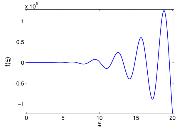
Figure 1: (Color online) The function $f(\xi)$ ($\xi\equiv\frac{\omega a}{c}$), defined in Eq. (25), which determines the $a$-dependent part of the radiated power per unit area for a given mechanical frequency $\omega$.

The second particular case corresponds to a more immediate limit of the general result, and corresponds to $a\to\infty$ (we recall that the power is always evaluated at $x_{3}>>a$) and the result becomes independent of $x_{3}$). In this situation, we have:

$${\mathcal{P}}(\omega)\,\sim\,2|\omega||\tilde{q}(\omega)|^{2}\int_{0}^{\omega/c}dk_{\parallel}\,k_{\parallel}^{3}\;\sqrt{(\frac{\omega}{c})^{2}-k_{\parallel}^{2}}\;\widetilde{\Omega}(k_{\parallel})\;,$$ (26)

since the highly oscillating sine function (assuming $\widetilde{\Omega}$ to be a smooth function of its argument) can be approximated by $1/2$. This corresponds again to twice the result in the absence of the conducting plane, and for the same reason. It is also self-evident that all the resonant phenomena disappear in this limit.

Using the sharp-cutoff model for the autocorrelation function ${\tilde{\Omega}}(k_{\parallel})$ (with $k_{\rm max}>\omega/c$) it is possible to find that the power in (26) is ${\mathcal{P}}(\omega)\sim|\tilde{q}(\omega)|^{2}\omega^{6}/c^{5}$. This case, can be compared with that coming from the DCE FLM2013 , since a single accelerated perfect mirror creates photons due to the interaction with the quantum fluctuations of the electromagnetic field. Just considering dimensional arguments, and limiting the analysis to the non-relativistic case, one expect that the dissipative force per unit length on the mirror to be proportional to $\dddot{a}/c^{4}$. This force corresponds to a spectral density ${\mathcal{P}}_{\rm DCE}(\omega)\sim|\tilde{q}(\omega)|^{2}\omega^{6}/c^{4}$ reviews dce .

Finally, as the final limiting case we see that the radiated energy also vanishes when the correlation length is infinite. This result can be understood by applying Gauss law for ${\mathbf{E}}$, on a large closed box with two of its faces parallel to the planes, taking into account the fact that the total electric charge is zero.

III Patch potentials

III.1 The system

Let us consider the second model, again assuming the motion to be non-relativistic. The moving plane is assumed to have a patch potential distribution on its side facing the static mirror.

Now, the patch potentials may be constructed by introducing two dipole layers close to the moving plane. One of them represents the patch potential itself, and is located at $x_{3}=\psi^{-}(t)$, $\psi^{-}\equiv\psi-\epsilon$ ($\epsilon$ a positive infinitesimal). The other, its image, is introduced in order to have perfect conductor boundary conditions at $x_{3}=\psi(t)$; therefore it is located at $\psi^{+}\equiv\psi+\epsilon$. Leaving aside for the moment the existence of perfect boundary conditions at $x_{3}=0$, we have the charge and current densities $\rho_{P}({\mathbf{x}},t)$ and ${\mathbf{j}}_{P}({\mathbf{x}},t)$, respectively:

$$\rho_{P}({\mathbf{x}},t) = -D({\mathbf{x}}_{\parallel})\,\big{[}\delta^{\prime}(x_{3}-\psi^{-}(t))+\delta^{\prime}(x_{3}-\psi^{+}(t))\big{]}\;\,,$$

$${\mathbf{j}}_{P}({\mathbf{x}},t) = -D({\mathbf{x}}_{\parallel})\,\big{[}\delta^{\prime}(x_{3}-\psi^{-}(t))+\delta^{\prime}(x_{3}-\psi^{+}(t))\big{]}\,{\dot{\psi}}(t)\,\mathbf{\hat{e}_{3}}\;.$$ (27)

In order to satisfy perfect conductor boundary conditions at $x_{3}=0$, we must introduce now an infinite number of images which mirror the previous sources (at the appropriate locations). Is is straightforward to see that the full charge and current densities which ensure the proper boundary conditions to hold true, are given by:

$$\rho({\mathbf{x}},t) = -D({\mathbf{x}}_{\parallel})\,\sum_{n=-\infty}^{+\infty}\big{[}\delta^{\prime}(x_{3}-\psi_{n}^{-}(t))+\delta^{\prime}(x_{3}-\psi_{n}^{+}(t))\big{]}\;\,,$$

$${\mathbf{j}}({\mathbf{x}},t) = -D({\mathbf{x}}_{\parallel})\,\sum_{n=-\infty}^{+\infty}\big{[}\delta^{\prime}(x_{3}-\psi_{n}^{-}(t))+\delta^{\prime}(x_{3}-\psi_{n}^{+}(t))\big{]}\,\,{\dot{\psi}}_{n}(t)\,\mathbf{\hat{e}_{3}}\;,$$ (28)

where: $\psi_{n}(t)\equiv(2n+1)\psi(t)$, and $\psi_{n}^{\pm}(t)\equiv(2n+1)\psi^{\pm}(t)$ .

It is convenient, for later use, to note that the charge and current densities above may be written as follows:

$$\rho({\mathbf{x}},t)\,=\,-D({\mathbf{x}}_{\parallel})\,\frac{\partial\sigma}{\partial x_{3}}(x_{3},t)\;\;,\;{\mathbf{j}}({\mathbf{x}},t)\,=\,D({\mathbf{x}}_{\parallel})\,\frac{\partial\sigma}{\partial t}(x_{3},t)\,\mathbf{\hat{e}_{3}}\;,$$ (29)

with:

$$\sigma(x_{3},t)\;=\;\sum_{n=-\infty}^{+\infty}\big{[}\delta(x_{3}-\psi_{n}^{-}(t))+\delta(x_{3}-\psi_{n}^{+}(t))\big{]}\;.$$ (30)

III.2 Mechanical power per unit area on the moving plate

There is no radiation outside of the volume enclosed by the two plates, but there may be energy traded between the EM field and the environment, by means of the mechanical work exerted on the moving mirror. The rate of change of ${\mathcal{E}}(t)$, the total energy per unit area contained between the static and moving planes, is given by:

$$\frac{d{\mathcal{E}}}{dt}(t)\;=\;\dot{\psi}(t)\,f(t)$$ (31)

where $f(t)$ denotes the $x_{3}$ component of the force per unit area on the moving plate. This is in turn obtained as follows:

$$f(t)\;=\;\int d^{2}{\mathbf{x}}_{\parallel}\,\big{[}T_{33}({\mathbf{x}}_{\parallel},\psi^{+}(t),t)\,-\,T_{33}({\mathbf{x}}_{\parallel},\psi^{-}(t),t)\big{]}$$ (32)

where $T_{ij}$ is Maxwell’s stress tensor.

In terms of the potentials, $T_{33}$, the only relevant component of $T_{ij}$ for this calculation, may be written as follows:

$$T_{33}\;=\;-\frac{1}{8\pi}\,\Big{[}(\partial_{j}\partial_{3}\chi)^{2}\,+\,\frac{1}{c^{2}}(\partial_{j}\partial_{t}\chi)^{2}\,-\,(\partial_{3}^{2}\chi+\frac{1}{c^{2}}\partial_{t}^{2}\chi)^{2}\Big{]}\;.$$ (33)

where we have used the property that the potentials may be written (for the kind of sources that we are considering) as follows:

$$\phi\;=\;-\frac{\partial\chi}{\partial x_{3}}\;\;,\;\;\;\;A_{3}\;=\;\frac{1}{c}\frac{\partial\chi}{\partial t}\;,$$ (34)

where the scalar function $\chi$ can be written in terms of the retarded Green’s function $G$:

$$\chi({\mathbf{x}},t)\;=\;\int d^{3}{\mathbf{x}^{\prime}}\int dt^{\prime}\;G({\mathbf{x}},t;{\mathbf{x}^{\prime}},t^{\prime})\,D({\mathbf{x}^{\prime}_{\parallel}})\sigma(x^{\prime}_{3},t^{\prime})\;,$$ (35)

with $\sigma(x_{3},t)$ as introduced previously in (30).

The perturbative expansion for $\frac{d{\mathcal{E}}(t)}{dt}=\dot{\mathcal{E}}(t)$, in powers of $q(t)$ has the form

$$\dot{\mathcal{E}}(t)\;=\;\dot{\mathcal{E}}^{(0)}(t)\,+\,\dot{\mathcal{E}}^{(1)}(t)\,+\,\dot{\mathcal{E}}^{(2)}(t)\,+\,\ldots$$ (36)

where the index denotes the order of the corresponding term. Since $\dot{\psi}$ is of order $1$, we see that:

$$\dot{\mathcal{E}}^{(0)}\;=\;0\;\;,\;\;$$ (37)

as it should be, since at the zeroth order both planes are static, and therefore there can be no power.

Regarding the first-order term, one clearly has the relation:

$$\dot{\mathcal{E}}^{(1)}\;=\;\dot{\psi}(t)\,f^{(0)}\;,$$ (38)

where $f^{(0)}$ denotes the zeroth order force per unit area for a static system. Thus, the previous equation may be integrated out to obtain:

$$\delta{\mathcal{E}}\;=\;\delta a\,f^{(0)}\;,$$ (39)

in other words, $f^{(0)}=(\frac{\partial{\mathcal{E}}}{\partial a})^{(0)}$. The explicit evaluation of $f^{(0)}$ yields:

$$f^{(0)}\;=\;8\pi\,\int\frac{d^{2}{\mathbf{k}}_{\parallel}}{(2\pi)^{2}}\,|{\mathbf{k}}_{\parallel}|^{2}\,{\widetilde{\Omega}}({\mathbf{k}}_{\parallel})\,\Big{[}\frac{1}{e^{2|{\mathbf{k}}_{\parallel}|a}-1}+\frac{1}{(e^{2|{\mathbf{k}}_{\parallel}|a}-1)^{2}}\Big{]}\;,$$ (40)

which agrees with the force one would obtain from the static interaction energy resulting between two conductors with patch potentials FLM2013 .

The second order term, requires the calculation of $f^{(1)}$:

$$\dot{\mathcal{E}}^{(2)}\;=\;\dot{\psi}(t)\,f^{(1)}(t)\;.$$ (41)

We see that:

$$f^{(1)}(t)\;=\;\frac{1}{4\pi}\,\lim_{L\to\infty}\frac{1}{L^{2}}\,\int_{-L/2}^{+L/2}dx_{1}\int_{-L/2}^{+L/2}dx_{2}\,\Big{\{} -\big{[}\partial_{j}\partial_{3}\chi(x_{1},x_{2},\psi^{-}(t),t)\big{]}^{(0)}\big{[}\partial_{j}\partial_{3}\chi(x_{1},x_{2},\psi^{-}(t),t)\big{]}^{(1)}$$ (42)

$$-\big{[}\frac{1}{c}\partial_{j}\partial_{t}\chi(x_{1},x_{2},\psi^{-}(t),t)\big{]}^{(0)}\big{[}\frac{1}{c}\partial_{j}\partial_{t}\chi(x_{1},x_{2},\psi^{-}(t),t)\big{]}^{(1)}$$ (43)

$$+\big{[}\partial_{3}^{2}\chi(x_{1},x_{2},\psi^{-}(t),t)-\frac{1}{c^{2}}\partial_{t}^{2}\chi(x_{1},x_{2},\psi^{-}(t),t)\big{]}^{(0)}$$ (44)

$$\times\big{[}\partial_{3}^{2}\chi(x_{1},x_{2},\psi^{-}(t),t)-\frac{1}{c^{2}}\partial_{t}^{2}\chi(x_{1},x_{2},\psi^{-}(t),t)\big{]}^{(1)}\Big{\}}\;.$$ (45)

It is rather straightforward to show that the first two terms on the rhs of the equation above vanish. Thus, keeping only the third term, and introducing Fourier transforms, we see that:

$$f^{(1)}(t)=\frac{1}{4\pi}\,\int\frac{d^{2}{\mathbf{k}}_{\parallel}}{(2\pi)^{2}}\,{\widetilde{\Omega}}({\mathbf{k}}_{\parallel})\,F_{1}({\mathbf{k}}_{\parallel},a)\;F_{2}({\mathbf{k}}_{\parallel},a,t)\;,$$ (46)

where we have introduced:

$$F_{1}({\mathbf{k}}_{\parallel},a)\;\equiv\;\int\frac{dk_{3}}{2\pi}\int\frac{d\omega}{2\pi}\,e^{i(k_{3}a^{-}-\omega t)}\,\widetilde{G}({\mathbf{k}}_{\parallel},k_{3},0)\,k_{3}^{2}\,\widetilde{\sigma}^{(0)}(k_{3},\omega)\;,$$ (47)

and

$$F_{2}({\mathbf{k}}_{\parallel},a,t)\;\equiv\;\int\frac{dk_{3}}{2\pi}\int\frac{d\omega}{2\pi}\,e^{i(k_{3}a^{-}-\omega t)}\,\widetilde{G}({\mathbf{k}}_{\parallel},k_{3},\omega)\,[k_{3}^{2}-(\frac{\omega}{c})^{2}]\,\widetilde{\sigma}^{(1)}(k_{3},\omega)\;.$$ (48)

Using the explicit form of the Green’s functions, $\sigma$, and of their Fourier transforms, we find after some algebra:

$$F_{1}({\mathbf{k}}_{\parallel},a)\;=\;-4\pi\;|{\mathbf{k}}_{\parallel}|\;\coth(|{\mathbf{k}}_{\parallel}|a)\;,$$ (49)

while for $F_{2}$ the result may be put in the form:

$$F_{2}({\mathbf{k}}_{\parallel},a,t)=\frac{4\pi}{a^{2}}\,|{\mathbf{k}}_{\parallel}|^{2}\,\,(-1+a\frac{d}{da})\sum_{-\infty}^{+\infty}\int\frac{d\omega}{2\pi}\,\,e^{-i\omega t}\frac{\tilde{q}(\omega)}{(\frac{n\pi}{a})^{2}+{\mathbf{k}}_{\parallel}^{2}-(\frac{\omega+i\eta}{c})^{2}}\;.$$ (50)

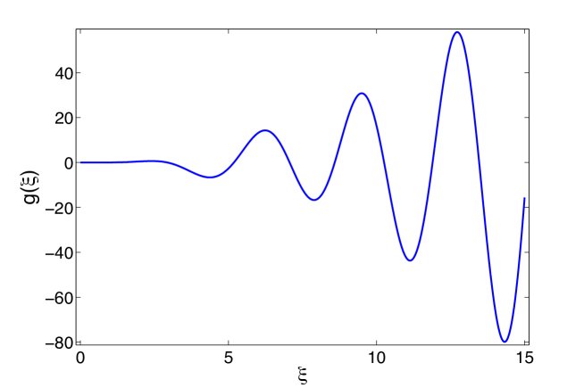
Figure 2: (Color online) The function $g(\xi)$ ($\xi\equiv\frac{\omega a}{c}$), defined for a given mechanical frequency $\omega$. Parameters of the autocorrelation function are $k_{\rm min}=0$ and $k_{\rm max}>\omega/c$.

We have discarded in $F_{2}$ an infinite (additive) contribution which is proportional to $q(t)$. This divergence is due to the zero with of the mirrors, and can naturally be interpreted as a renormalization of the self-energy of the moving mirror. Besides, note that is not related to dissipation, since the force is conservative, and can be derived from a harmonic potential.

In order to gain some insight into the nature of the system, we now write $f^{(1)}$ in Fourier (frequency) representation,

$$\widetilde{f^{(1)}}(\omega)\;=\;\frac{4\pi}{a^{2}}\,\tilde{q}(\omega)\;\int\frac{d^{2}{\mathbf{k}}_{\parallel}}{(2\pi)^{2}}\,{\widetilde{\Omega}}({\mathbf{k}}_{\parallel})\,|{\mathbf{k}}_{\parallel}|^{3}\,\coth(|{\mathbf{k}}_{\parallel}|a)\,(1-a\frac{d}{da})\,\sum_{-\infty}^{+\infty}\frac{1}{(\frac{n\pi}{a})^{2}+{\mathbf{k}}_{\parallel}^{2}-(\frac{\omega+i\eta}{c})^{2}}\;.$$ (51)

Performing the summation, assuming rotational invariance for $\widetilde{\Omega}$, and keeping just the dissipative terms, we see that

$$\widetilde{f^{(1)}}(\omega)\;=\;2\,\tilde{q}(\omega)\;\int_{0}^{\omega}dk_{\parallel}{\widetilde{\Omega}}(k_{\parallel})\,k_{\parallel}^{4}\,\coth(k_{\parallel}a)\,\csc^{2}(\sqrt{\omega^{2}-k_{\parallel}^{2}}a)\;.$$ (52)

We write this expression in terms of a new function,

$$\widetilde{f^{(1)}}(\omega)=\tilde{q}(\omega)\;g(\xi)\;,$$ (53)

where, again, $\xi=\omega a/c$. In Fig. 2 we show the function $g(\xi)$ for the two-cutoff model autocorrelation function in which, for the sake of simplicity, we have set $k_{\rm min}=0$ and $k_{\rm max}>\omega/c$. Again, the existence of resonances is evident. As in the case of the first example, we see that bigger frequencies are able to excite all the normal frequencies ($\sqrt{(\frac{n\pi}{a})^{2}+|{\mathbf{k}}_{\parallel}|^{2}}$) which are smaller than $\omega$. That explains the fact that the peaks grow with the frequency.

Finally, as another manifestation of the same effect, we can derive the spectral density of the power (to the second order in $q$):

$$\widetilde{\dot{\mathcal{E}}^{(2)}}(\omega)\,=\,\int_{0}^{\infty}\frac{d\omega}{2\pi}\,{\mathcal{P}}(\omega)$$ (54)

which has a rather similar interpretation to the one we calculated in the previous example. Its form can be obtained explicitly by performing the integration, the result being:

$${\mathcal{P}}(\omega)\;=\;\frac{8\pi}{a^{2}}c^{2}\,|\tilde{q}(\omega)|^{2}\,\int\frac{d^{2}{\mathbf{k}}_{\parallel}}{(2\pi)^{2}}\,{\widetilde{\Omega}}({\mathbf{k}}_{\parallel})\,|{\mathbf{k}}_{\parallel}|^{3}\,\coth(|{\mathbf{k}}_{\parallel}|a)\,(1-a\frac{d}{da})\,\sum_{-\infty}^{+\infty}\delta\big{[}\omega-\sqrt{(\frac{n\pi}{a})^{2}+|{\mathbf{k}}_{\parallel}|^{2}}\big{]}\;.$$ (55)

The presence of the resonances is again evident, now in the $\delta$-functions. The position of the resonances agrees with the ones determined in Ref. Kardar:1997cu within the context of the DCE, for a quantum system with a similar geometry but corresponding to a quantum real scalar field.

IV Conclusions

We have presented results about the spectrum of the radiation generated by two closely related systems, containing a planar dipole layer distribution which oscillates in front of a conducting plane, in terms of the layer autocorrelation function. In one of the systems, where the layer on the moving plane is meant to describe a dielectric with permanent polarization, we have found that the radiated power exhibits enhancements for certain frequencies of oscillation. We interpret them as being related to the existence of constructive interference between the radiation generated by the layer and the one that bounces on the conductor before reaching a given point.

In the other system, the moving plane also has conductor boundary conditions on the face opposite to the static plane, and is used to describe patch potentials. The extra boundary condition makes it possible to have infinite bounces, and therefore resonances, which we have plotted for a simple autocorrelation function. The physical observables considered for this case were the force exerted on the moving plane, and its power.

References

- (1) For recent reviews see The nonstationary Casimir effect and quantum systems with moving boundaries, G. Barton, V.V. Dodonov and V.I. Manko (editors), J. Opt. B: Quantum Semiclass. Opt.7 S1 (2005). V. V. Dodonov, Phys. Scripta 82 (2010) 038105; D. A. R. Dalvit, P. A. Maia Neto and F. D. Mazzitelli, Lect. Notes Phys. 834 (2011) 419.
- (2) P. C. W. Davies and S. A. Fulling, Proc. Roy. Soc. Lond. A 348, 393 (1976).
- (3) C. D. Fosco and F. D. Mazzitelli, Phys. Rev. A 89, 062513 (2014).
- (4) C. C. Speake and C. Trenkel, Phys. Rev. Lett. 90, 160403 (2003).
- (5) R. O. Behunin, D. A. R. Dalvit, R. S. Decca, and C. C. Speake, Phys. Rev. D 89, 051301(R) (2014).
- (6) J.R. Ellis, Proc. Cambridge Philos. Soc. 59, 759 (1963); G.N. Ward, Proc. R. Soc. London A 279, 562 (1964): Proc. Cambridge Philos. Soc. 61, 547 (1965); J.J. Monaghan, J. Phys. A 1, 112 (1968).
- (7) J.A. Heras, Am. J. Phys. 62 1109, (1994).
- (8) R. Smoluchowski, Phys. 60, 661 (1941); N. D. Lang and W. Kohn, Phys. Rev. B 3, 1215 (1971); N. Gaillard et. al., Appl. Phys. Lett. 89, 154101 (2006).
- (9) S.E. Pollack, S. Schlamminger and J.H. Gundlach, Phys. Rev. Lett. 101, 071101 (2008); L. Deslauriers, et al, Phys. Rev. Lett. 97, 103007 (2006); J.D. Carter and J.D.D. Martin, Phys. Rev. A 83, 032902 (2011).
- (10) C. D. Fosco, F. C. Lombardo, and F. D. Mazzitelli, Phys. Rev. A 88, 062501 (2013).
- (11) M. Kardar and R. Golestanian, Rev. Mod. Phys. 71, 1233 (1999).