Complex Line Bundles over Simplicial Complexes and their Applications

Abstract.

Discrete vector bundles are important in Physics and recently found remarkable applications in Computer Graphics. This article approaches discrete bundles from the viewpoint of Discrete Differential Geometry, including a complete classification of discrete vector bundles over finite simplicial complexes. In particular, we obtain a discrete analogue of a theorem of André Weil on the classification of hermitian line bundles. Moreover, we associate to each discrete hermitian line bundle with curvature a unique piecewise-smooth hermitian line bundle of piecewise constant curvature. This is then used to define a discrete Dirichlet energy which generalizes the well-known cotangent Laplace operator to discrete hermitian line bundles over Euclidean simplicial manifolds of arbitrary dimension.

1. Introduction

Vector bundles are fundamental objects in Differential Geometry and play an important role in Physics [2]. The Physics literature is also the main place where discrete versions of vector bundles were studied: First, there is a whole field called Lattice Gauge Theory where numerical experiments concerning connections in bundles over discrete spaces (lattices or simplicial complexes) are the main focus. Some of the work that has been done in this context is quite close to the kind of problems we are going to investigate here [3, 4, 6].

Vector bundles make their most fundamental appearance in Physics in the form of the complex line bundle whose sections are the wave functions of a charged particle in a magnetic field. Here the bundle comes with a connection whose curvature is given by the magnetic field [2]. There are situations where the problem itself suggests a natural discretization: The charged particle (electron) may be bound to a certain arrangement of atoms. Modelling this situation in such a way that the electron can only occupy a discrete set of locations then leads to the “tight binding approximation” [12, 1, 17].

Recently vector bundles over discrete spaces also have found striking applications in Geometry Processing and Computer Graphics. We will describe these in detail in Section 2.

In order to motivate the basic definitions concerning vector bundles over simplicial complexes let us consider a smooth manifold $\tilde{\mathrm{M}}$ that comes with smooth triangulation (Figure 1).

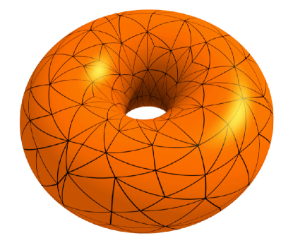
Figure 1. A smooth triangulation of a manifold.

Let $\tilde{\mathrm{E}}$ be a smooth vector bundle over $\tilde{\mathrm{M}}$ of rank $\mathfrak{K}$. Then we can define a discrete version $\mathrm{E}$ of $\tilde{\mathrm{E}}$ by restricting $\tilde{\mathrm{E}}$ to the vertex set $\mathcal{V}$ of the triangulation. Thus $\mathrm{E}$ assigns to each vertex $i\in\mathcal{V}$ the $\mathfrak{K}$-dimensional real vector space $\mathrm{E}_{i}:=\tilde{\mathrm{E}}_{i}$. This is the way vector bundles over simplicial complexes are defined in general: Such a bundle $\mathrm{E}$ assigns to each vertex $i$ a $\mathfrak{K}$-dimensional real vector space $\mathrm{E}_{i}$ in such a way that $\mathrm{E}_{i}\mathop{\cap}\mathrm{E}_{j}=\emptyset$ for $i\neq j$.

So far the notion of a discrete vector bundle is completely uninteresting mathematically: The obvious definition of an isomorphism between two such bundles $\mathrm{E}$ and $\hat{\mathrm{E}}$ just would require a vector space isomorphism $f_{i}\colon\mathrm{E}_{i}\to\hat{\mathrm{E}}_{i}$ for each vertex $i$. Thus, unless we put more structure on our bundles, any two vector bundles of the same rank over a simplicial complex are isomorphic.

Suppose now that $\tilde{\mathrm{E}}$ comes with a connection $\nabla$. Then we can use the parallel transport along edges $\ij$ of the triangulation to define vector space isomorphisms

$$\eta_{\ij}\colon\tilde{\mathrm{E}}_{i}\to\tilde{\mathrm{E}}_{j}$$

This leads to the standard definition of a connection on a vector bundle over a simplicial complex: Such a connection is given by a collection of isomorphisms $\eta_{\ij}\colon\mathrm{E}_{i}\to\mathrm{E}_{j}$ defined for each edge $\ij$ such that

$$\eta_{ji}=\eta_{\ij}^{-1}.$$

Now the classification problem becomes non-trivial because for an isomorphism $f$ between two bundles $\mathrm{E}$ and $\hat{\mathrm{E}}$ with connection we have to require compatibility with the transport maps $\eta_{\ij}$:

$$f_{j}\circ\eta_{\ij}=\hat{\eta}_{\ij}\circ f_{i}.$$

Given a connection $\eta$ and a closed edge path $\gamma=e_{\ell}\cdots e_{1}$ (compare Section 4) of the simplicial complex we can define the monodromy $P_{\gamma}\in\mathrm{Aut}(\mathrm{E}_{i})$ around $\gamma$ as

$$P_{\gamma}=\eta_{e_{\ell}}\circ\ldots\circ\eta_{e_{1}}.$$

In particular the monodromies around triangular faces of the simplicial complex provide an analog for the smooth curvature in the discrete setting. In Section 4 we will classify vector bundles with connection in terms of their monodromies.

Let us look at the special case of a rank $2$ bundle $\mathrm{E}$ that is oriented and comes with a Euclidean scalar product. Then the $90^{\circ}$-rotation in each fiber makes it into $1$-dimensional complex vector space, so we effectively are dealing with a hermitian complex line bundle. If $ijk$ is an oriented face of our simplicial complex, the monodromy $P_{\partial\,ijk}\colon\mathrm{E}_{i}\to\mathrm{E}_{i}$ around the triangle $ijk$ is multiplication by a complex number $h_{ijk}$ of norm one. Writing $h_{ijk}=e^{\imath\alpha_{ijk}}$ with $-\pi<\alpha_{ijk}\leq\pi$ we see that this monodromy can also be interpreted as a real curvature $\alpha_{ijk}\in(-\pi,\pi]$. It thus becomes apparent that the information provided by the connection $\eta$ cannot encode any curvature that integrated over a single face is larger than $\pm\pi$. This can be a serious restriction for applications: We effectively see a cutoff for the curvature that can be contained in a single face.

Remember however our starting point: We asked for structure that can be naturally transferred from the smooth setting to the discrete one. If we think again about a triangulated smooth manifold it is clear that we can associate to each two-dimensional face $ijk$ the integral $\Omega_{ijk}$ of the curvature $2$-form over this face. This is just a discrete $2$-form in the sense of discrete exterior calculus [5]. Including this discrete curvature $2$-form with the parallel transport $\eta$ brings discrete complex line bundles much closer to their smooth counterparts:

Definition: A hermitian line bundle with curvature over a simplicial complex $\mathcal{X}$ is a triple $(\mathrm{E},\eta,\Omega)$. Here $\mathrm{E}$ is complex hermitian line bundle over $\mathcal{X}$, for each edge $\ij$ the maps $\eta_{\ij}\colon\mathrm{E}_{i}\to\mathrm{E}_{j}$ are unitary and the closed real-valued $2$-form $\Omega$ on each face $ijk$ satisfies

$$\eta_{ki}\circ\eta_{jk}\circ\eta_{\ij}=e^{\imath\Omega_{ijk}}\,\mathrm{id}_{\mathrm{E}_{i}}.$$

In Section 7 we will prove for hermitian line bundles with curvature the discrete analog of a well-known theorem by André Weil on the classification of hermitian line bundles.

In Section 8 we will define for hermitian line bundles with curvature a degree (which can be an arbitrary integer) and we will prove a discrete version of the Poincaré-Hopf index theorem concerning the number of zeros of a section (counted with sign and multiplicity).

Finally we will construct in Section 10 for each hermitian line bundle with curvature a piecewise-smooth bundle with a curvature $2$-form that is constant on each face. Sections of the discrete bundle can be canonically extended to sections of the piecewise-smooth bundle. This construction will provide us with finite elements for bundle sections and thus will allow us to compute the Dirichlet energy on the space of sections.

2. Applications of Vector Bundles in Geometry Processing

Several important tasks in Geometry Processing (see the examples below) lead to the problem of coming up with an optimal normalized section $\phi$ of some Euclidean vector bundle $\mathrm{E}$ over a compact manifold with boundary $\mathrm{M}$. Here “normalized section” means that $\phi$ is defined away from a certain singular set and where defined it satisfies $|\phi|=1$.

In all the mentioned situations $\mathrm{E}$ comes with a natural metric connection $\nabla$ and it turns out that the following method for finding $\phi$ yields surprisingly good results:

Among all sections $\psi$ of $\mathrm{E}$ find one which minimizes $\int_{\mathrm{M}}|\nabla\psi|^{2}$ under the constraint $\int_{\mathrm{M}}|\psi|^{2}=1$. Then away from the zero set of $\psi$ use $\phi=\psi/|\psi|$.

The term ”optimal” suggests that there is a variational functional which is minimized by $\phi$ and this is in fact the case. Moreover, in each of the applications there are heuristic arguments indicating that $\phi$ is indeed a good choice for the problem at hand. For the details we refer to the original papers. Here we are only concerned with the Discrete Differential Geometry involved in the discretization of the above variational problem.

2.1. Direction Fields on Surfaces

Here $\mathrm{M}$ is a surface with a Riemannian metric, $\mathrm{E}=\mathrm{TM}$ is the tangent bundle and $\nabla$ is the Levi-Civita connection. Figure 2 shows the resulting unit vector field $\phi$.

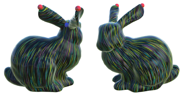
Figure 2. An optimal direction field on a surface.

If we consider $\mathrm{TM}$ as a complex line bundle, normalized sections of the tensor square $\mathrm{L}=\mathrm{TM}\otimes\mathrm{TM}$ describe unoriented direction fields on $\mathrm{M}$. Similarly, “higher order direction fields” like cross fields are related to higher tensor powers of $\mathrm{TM}$. Higher order direction fields also have important applications in Computer Graphics.

2.2. Stripe Patterns on Surfaces

A stripe pattern on a surface $\mathrm{M}$ is a map which away from a certain singular set assigns to each point $p\in\mathrm{M}$ an element $\phi(p)\in\mathbb{S}=\{z\in\mathbb{C}||z|=1\}$. Such a map $\phi$ can be used to color $\mathrm{M}$ in a periodic fashion according to a color map that assigns a color to each point on the unit circle $\mathbb{S}$. Suppose we are given a $1$-form $\omega$ on $\mathrm{M}$ that specifies a desired direction and spacing of the stripes, which means that ideally we would wish for something like $\phi=e^{i\alpha}$ with $d\alpha=\omega$. Then the algorithm in [9] says that we should use a $\phi$ that comes from taking $\mathrm{E}$ as the trivial bundle $\mathrm{E}=\mathrm{M}\times\mathbb{C}$ and $\nabla\psi=d\psi-i\omega\psi$. Sometimes the original data come from an unoriented direction field and (in order to obtain the $1$-form $\omega$) we first have to move from $\mathrm{M}$ to a double branched cover $\tilde{\mathrm{M}}$ of $\mathrm{M}$. This is for example the case in Figure 3.

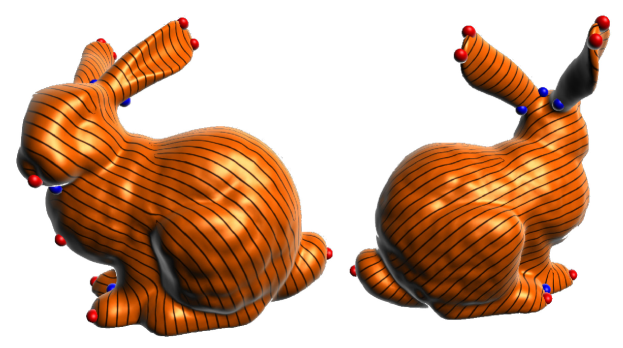
Figure 3. An optimal stripe pattern aligned to an unoriented direction field.

2.3. Decomposing Velocity Fields into Fields Generated by Vortex Filaments

The velocity fields that arise in fluid simulations quite often can be understood as a superposition of interacting vortex rings. It is therefore desirable to have an algorithm that reconstructs the underlying vortex filaments from a given velocity field. Let the velocity field $\mathbf{v}$ on a domain $\mathrm{M}\subset\mathbb{R}^{3}$ be given as a $1$-form $\omega=\langle\mathbf{v},\cdot\rangle$. Then the algorithm proposed in [20] uses the function $\phi\colon\mathrm{M}\to\mathbb{C}$ that results from taking the trivial bundle $\mathrm{E}=\mathrm{M}\times\mathbb{C}$ endowed with the connection $\nabla\psi=d\psi-i\omega\psi$. Note that so far this is just a three-dimensional version of the situation in Section 2.2. This time however we even forget $\phi$ in the end and only retain the zero set of $\psi$ as the filament configuration we are looking for.

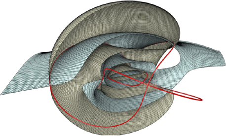
Figure 4. A knotted vortex filament defined as the zero set of a complex valued function $\psi$. It is shown as the intersection of the zero set of $\real\,\psi$ with the zero set of $\mathrm{Im}\,\psi$.

2.4. Close-To-Conformal Deformations of Volumes

Here the data are a domain $\mathrm{M}\subset\mathbb{R}^{3}$ and a function $u\colon\mathrm{M}\to\mathbb{R}$. The task is to find a map $f\colon\mathrm{M}\to\mathbb{R}^{3}$ which is approximately conformal with conformal factor $e^{u}$, i.e. for all tangent vectors $X\in\mathrm{TM}$ we want

$$|df(X)|\approx e^{u}|X|.$$

The only exact solutions of this equations are the Möbius transformations. For these we find

$$df(X)=e^{u}\overline{\psi}X\psi$$

for some map $\psi\colon\mathrm{M}\to\mathbb{H}$ with $|\psi|=1$ which in addition satisfies

$$d\psi(X)=-\tfrac{1}{2}(\mathrm{grad}\,u\times X)\,\psi.$$

Note that here we have identified $\mathbb{R}^{3}$ with the space of purely imaginary quaternions. Let us define a connection $\nabla$ on the trivial rank $4$ vector bundle $\mathrm{M}\times\mathbb{H}$ by

$$\nabla_{X}\psi:=d\psi(X)+\tfrac{1}{2}(\mathrm{grad}\,u\times X)\psi.$$

Then we can apply the usual method and find a section $\phi\colon\mathrm{M}\to\mathbb{H}$ with $|\phi|=1$. In general there will not be any $f\colon\mathrm{M}\to\mathbb{R}^{3}$ that satisfies

(2.1) $$df(X)=e^{u}\overline{\phi}X\phi$$

exactly but we can always look for an $f$ that satisfies (2.1) in the least squares sense. See Figure 5 for an example.

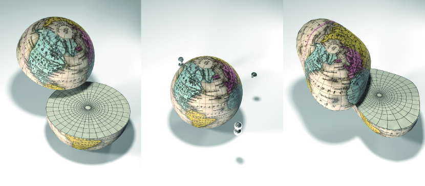
Figure 5. Close-to-conformal deformation of a sphere based on a desired conformal factor specified as the potential of a collection of point charges.

3. Discrete Vector Bundles with Connection

An (abstract) simplicial complex is a collection $\mathcal{X}$ of finite non-empty sets such that if $\sigma$ is an element of $\mathcal{X}$ so is every non-empty subset of $\sigma$ ([15]).

An element of a simplicial complex $\mathcal{X}$ is called a simplex and each non-empty subset of a simplex $\sigma$ is called a face of $\sigma$. The elements of a simplex are called vertices and the union of all vertices $\mathcal{V}=\mathop{\cup}_{\sigma\in\mathcal{X}}\sigma$ is called the vertex set of $\mathcal{X}$. The dimension of a simplex is defined to be one less than the number of its vertices: $\dim\sigma:=|\sigma|-1$. A simplex of dimension $k$ is also called a $k$-simplex. The dimension of a simplicial complex is defined as the maximal dimension of its simplices.

To avoid technical difficulties, we will restrict our attention to finite simplicial complexes only. The main concepts are already present in the finite case. Though, the definitions carry over verbatim to infinite simplicial complexes.

Definition 1.

Let $\mathbb{F}$ be a field and let $\mathcal{X}$ be a simplicial complex with vertex set $\mathcal{V}$. A discrete $\mathbb{F}$-vector bundle of rank $\mathfrak{K}\in\mathbb{N}$ over $\mathcal{X}$ is a map $\pi\colon\mathrm{E}\to\mathcal{V}$ such that for each vertex $i\in\mathcal{V}$ the fiber over $i$

$$\mathrm{E}_{i}:=\pi^{-1}(\{i\})$$

has the structure of a $\mathfrak{K}$-dimensional $\mathbb{F}$-vector space.

Most of the time, we slightly abuse notation and denote a discrete vector bundle over a simplicial complex schematically by $\mathrm{E}\to\mathcal{X}$.

The usual vector space constructions carry fiberwise over to discrete vector bundles. So we can speak of tensor products or dual bundles. Moreover, the fibers can be equipped with additional structures. In particular, a real vector bundle whose fibers are Euclidean vector spaces is called a discrete Euclidean vector bundle. Similarly, a complex vector bundle whose fibers are hermitian vector spaces is called a discrete hermitian vector bundle.

So far discrete vector bundles are completely uninteresting from the mathematical viewpoint – the obvious definition of an isomorphism $f$ between two discrete vector bundles $\mathrm{E}$ and $\tilde{\mathrm{E}}$ just requires isomorphisms between the fibers $f_{i}\colon\mathrm{E}_{i}\to\tilde{\mathrm{E}}_{i}$. Thus any two bundles of rank $\mathfrak{K}$ are isomorphic. This changes if we connect the fibers along the edges by isomorphisms.

Let $\sigma=\{i_{0},\ldots,i_{k}\}$ be a $k$-simplex. We define two orderings of its vertices to be equivalent if they differ by an even permutation. Such an equivalence class is then called an orientation of $\sigma$ and a simplex together with an orientation is called an oriented simplex. We will denote the oriented $k$-simplex just by the word $i_{0}\cdots i_{k}$. Further, an oriented $1$-simplex is called an edge.

Definition 2.

Let $\mathrm{E}\to\mathcal{X}$ be a discrete vector bundle over a simplicial complex. A discrete connection on $\mathrm{E}$ is a map $\eta$ which assigns to each edge $\ij$ an isomorphism $\eta_{\ij}\colon\mathrm{E}_{i}\to\mathrm{E}_{j}$ of vector spaces such that

$$\eta_{ji}=\eta_{\ij}^{-1}.$$

Remark 1:

Here and in the following a morphism of vector spaces is a linear map that also preserves all additional structures - if any present. E.g., if we are dealing with hermitian vector spaces, then a morphism is a complex-linear map that preserves the hermitian metric, i.e. it is a complex linear isometric immersion.

Definition 3.

A morphism of discrete vector bundles with connection is a map $f\colon\mathrm{E}\to\mathrm{F}$ between discrete vector bundles $\mathrm{E}\to\mathcal{X}$ and $\mathrm{F}\to\mathcal{X}$ with connections $\eta$ and $\theta$ (resp.) such that

1. for each vertex $i$ we have that $f(\mathrm{E}_{i})\subset\mathrm{F}_{i}$ and the map $f_{i}=\left.f\right|_{\mathrm{E}_{i}}\colon\mathrm{E}_{i}\to\mathrm{F}_{i}$ is a morphism of vector spaces,

2. for each edge $\ij$ the following diagram commutes:

   

   ,

   i.e. $\theta_{\ij}\circ f_{i}=f_{j}\circ\eta_{\ij}$.

An isomorphism is a morphism which has an inverse map, which is also a morphism. Two discrete vector bundles with connection are called isomorphic, if there exists an isomorphism between them.

Again let $\mathcal{V}$ denote the vertex set of $\mathcal{X}$. A discrete vector bundle $\mathrm{E}\to\mathcal{X}$ with connection $\eta$ is called trivial, if it is isomorphic to the product bundle

$$\underline{\mathbb{F}^{\mathfrak{K}}}:=\mathcal{V}\times\mathbb{F}^{\mathfrak{K}}$$

over $\mathcal{X}$ equipped with the connection which assigns to each edge the identity $\mathrm{id}_{\mathbb{F}^{\mathfrak{K}}}$.

It is a natural question to ask how many non-isomorphic discrete vector bundles with connection exist on a given simplicial complex $\mathcal{X}$.

Remark 2:

For $k\in\mathbb{N}$, the $k$-skeleton $\mathcal{X}^{k}$ of a simplicial complex $\mathcal{X}$ is the subcomplex that consists of all simplices $\sigma\in\mathcal{X}$ of dimension $\leq k$,

$$\mathcal{X}^{k}:=\bigl{\{}\sigma\in\mathcal{X}\mid\dim\sigma\leq k\bigr{\}}.$$

The classification of vector bundles over $\mathcal{X}$ only involves its $1$-skeleton $\mathcal{X}^{1}$ and could be equally done just for discrete vector bundles over $1$-dimensional simplicial complexes, i.e. graphs. Later on, when we consider discrete hermitian line bundles with curvature in Section 7, the $2$- and $3$-skeleton come into play and finally, in Section 11, we will use the whole simplicial complex.

4. Monodromy - A Discrete Analogue of Kobayashi’s Theorem

Let $\mathcal{X}$ be a simplicial complex. Each edge $\ij$ of $\mathcal{X}$ has a start vertex $s(\ij):=i$ and a target vertex $t(\ij):=j$. A edge path $\gamma$ is a sequence of successive edges $(e_{1},\ldots,e_{\ell})$, i.e. $s(e_{k+1})=t(e_{k})$ for all $k=1,\ldots,\ell-1$, and will be denoted by the word:

$$\gamma=e_{\ell}\cdots e_{1}.$$

If $i=s(e_{1})$, we say that $\gamma$ starts at $i$, and if $j=t(e_{\ell})$ that $\gamma$ ends at $j$. The complex $\mathcal{X}$ is called connected, if any two of its vertices can be joined by an edge path. From now on we will only consider connected simplicial complexes.

Now, let $\mathrm{E}\to\mathcal{X}$ be a discrete vector bundle with connection $\eta$. To each edge path $\gamma=e_{\ell}\cdots e_{1}$ from $i$ to $j$, we define the parallel transport $P_{\gamma}\colon\mathrm{E}_{i}\to\mathrm{E}_{j}$ along $\gamma$ by

$$P_{\gamma}:=\eta_{e_{\ell}}\circ\cdots\circ\eta_{e_{1}}.$$

To each edge path $\gamma=e_{\ell}\cdots e_{1}$ we can assign an inverse path $\gamma^{-1}$. If $\tilde{\gamma}=e_{m}\cdots e_{\ell+1}$ starts where $\gamma$ ends, we can build the concatenation $\tilde{\gamma}\gamma$: With the notation $\ij^{-1}:=ji$, we have

$$\gamma^{-1}:=e_{1}^{-1}\cdots e_{\ell}^{-1},\quad\tilde{\gamma}\gamma:=e_{m}\cdots e_{\ell+1}e_{\ell}\cdots e_{1}.$$

Whenever $\tilde{\gamma}\gamma$ is defined,

(4.1) $$P_{\tilde{\gamma}\gamma}=P_{\tilde{\gamma}}\circ P_{\gamma},\quad P_{\gamma^{-1}}=P_{\gamma}^{-1}.$$

The elements of the fundamental group are identified with equivalence classes of edge loops, i.e. edge paths starting and ending a given base vertex $i$ of $\mathcal{X}$, where two such loops are identified if they differ by a sequence of elementary moves [SeifertThrelfall]:

$$e_{\ell}\cdots e_{k+1}e^{-1}e\,e_{k}\cdots e_{1}\longleftrightarrow e_{\ell}\cdots e_{k+1}e_{k}\cdots e_{1}.$$

Now, by Equation (4.1), we see that the parallel transport descends to a representation of the fundamental group $\pi_{1}(\mathcal{X}^{1},i)$. We encapsulate this in the following

Proposition 1.

Let $\mathrm{E}\to\mathcal{X}$ be a discrete vector bundle with connection over a connected simplicial complex. The parallel transport descends to a representation of the fundamental group $\pi_{1}(\mathcal{X}^{1},i)$:

$$\mathfrak{M}\colon\pi_{1}(\mathcal{X}^{1},i)\to\mathrm{Aut}(\mathrm{E}_{i}),\quad[\gamma]\mapsto P_{\gamma}.$$

The representation $\mathfrak{M}$ will be called the monodromy of the discrete vector bundle $\mathrm{E}$.

If we change the base vertex this leads to an isomorphic representation – an isomorphism is just given by the parallel transport $P_{\gamma}$ along an edge path joining the two base vertices. Moreover, if $f\colon\mathrm{E}\to\tilde{\mathrm{E}}$ is an isomorphism of discrete vector bundles with connection over the simplicial complex $\mathcal{X}$, for any edge path $\gamma=e_{\ell}\cdots e_{1}$ from a vertex $i$ to a vertex $j$ the following equality holds:

$$\tilde{P}_{\gamma}=f_{j}\circ P_{\gamma}\circ f_{i}^{-1}.$$

Here $P$ and $\tilde{P}$ denote the parallel transports of $\mathrm{E}$ and $\tilde{\mathrm{E}}$. Thus we obtain:

Proposition 2.

Isomorphic discrete vector bundles with connection have isomorphic monodromies.

In fact, the monodromy completely determines a discrete vector bundle with connection up to isomorphism, which provides a complete classification of discrete vector bundles with connection: Let $\mathcal{X}$ be a connected simplicial complex. Let $\mathrm{E}\to\mathcal{X}$ be a discrete $\mathbb{F}$-vector bundle of rank $\mathfrak{K}$ with connection and let $\mathfrak{M}\colon\pi_{1}(\mathcal{X}^{1},i)\to\mathrm{Aut}(\mathrm{E}_{i})$ denote its monodromy. Any choice of a basis of the fiber $\mathrm{E}_{i}$ determines a group homomorphism $\rho\in\mathrm{Hom}\bigl{(}\pi_{1}(\mathcal{X}^{1},i),\mathrm{GL}(\mathfrak{K},\mathbb{F})\bigr{)}$. Any other choice of basis determines a group homomorphism $\tilde{\rho}$ which is related to $\rho$ by conjugation, i.e. there is $S\in\mathrm{GL}(\mathfrak{K},\mathbb{F})$ such that

$$\tilde{\rho}([\gamma])=S\cdot\rho([\gamma])\cdot S^{-1}\textit{ for all }[\gamma]\in\pi_{1}(\mathcal{X}^{1},i).$$

Hence the monodromy $\mathfrak{M}$ determines a well-defined conjugacy class of group homomorphisms from $\pi_{1}(\mathcal{X}^{1},i)$ to $\mathrm{GL}(\mathfrak{K},\mathbb{F})$, which we will denote by $[\mathfrak{M}]$. The group $\mathrm{GL}(\mathfrak{K},\mathbb{F})$ will be referred to as the structure group of $\mathrm{E}$.

Let $\mathfrak{V}_{\mathbb{F}}^{\mathfrak{K}}(\mathcal{X})$ denote the set of isomorphism classes of $\mathbb{F}$-vector bundles of rank $\mathfrak{K}$ with connection over $\mathcal{X}$ and let $\mathrm{Hom}\bigl{(}\pi_{1}(\mathcal{X}^{1},i),\mathrm{GL}(\mathfrak{K},\mathbb{F})\bigr{)}/_{\sim}$ denote the set of conjugacy classes of group homomorphisms from the fundamental group $\pi_{1}(\mathcal{X}^{1},i)$ into the structure group $\mathrm{GL}(\mathfrak{K},\mathbb{F})$.

Theorem 1.

$F\colon\mathfrak{V}_{\mathbb{F}}^{\mathfrak{K}}(\mathcal{X})\to\mathrm{Hom}\bigl{(}\pi_{1}(\mathcal{X}^{1},i),\mathrm{GL}(\mathfrak{K},\mathbb{F})\bigr{)}/_{\sim}$, $[\mathrm{E}]\mapsto[\mathfrak{M}]$ is bijective.

Proof.

By Proposition 2, $F$ is well-defined. First we show injectivity. Consider two discrete vector bundles $\mathrm{E}$, $\tilde{\mathrm{E}}$ over $\mathcal{X}$ with connections $\eta$, $\tilde{\eta}$ and let $\mathfrak{M}$, $\tilde{\mathfrak{M}}$ denote their monodromies. Suppose that $[\mathfrak{M}]=[\tilde{\mathfrak{M}}]$. If we choose bases $\{X^{1}_{i},\ldots,X^{\mathfrak{K}}_{i}\}$ of $\mathrm{E}_{i}$ and $\{\tilde{X}^{1}_{i},\ldots,\tilde{X}^{\mathfrak{K}}_{i}\}$ of $\tilde{\mathrm{E}}_{i}$, then $\mathfrak{M}$ and $\tilde{\mathfrak{M}}$ are represented by group homomorphisms $\rho,\tilde{\rho}\in\mathrm{Hom}\bigl{(}\pi_{1}(\mathcal{X}^{1},i),\mathrm{GL}(\mathfrak{K},\mathbb{F})\bigr{)}$ which are related by conjugation. Without loss of generality, we can assume that $\rho=\tilde{\rho}$. Now, let $\mathcal{T}$ be a spanning tree of $\mathcal{X}$ with root $i$. Then for each vertex $j$ of $\mathcal{X}$ there is an edge path $\gamma_{\,i,j}$ from the root $i$ to the vertex $j$ entirely contained in $\mathcal{T}$. Since $\mathcal{T}$ contains no loops, the path $\gamma_{\,i,j}$ is essentially unique, i.e. any two such paths differ by a sequence of elementary moves. Thus we can use the parallel transport to obtain bases $\{X^{1}_{j},\ldots,X^{\mathfrak{K}}_{j}\}\subset\mathrm{E}_{j}$ and $\{\tilde{X}^{1}_{j},\ldots,\tilde{X}^{\mathfrak{K}}_{j}\}\subset\tilde{\mathrm{E}}_{j}$ at every vertex $j$ of $\mathcal{X}$. With respect to these bases the connections $\eta$ and $\tilde{\eta}$ are represented by elements of $\mathrm{GL}(\mathfrak{K},\mathbb{F})$. By construction, for each edge $e$ in $\mathcal{T}$ the connection is represented by the identity matrix. Moreover, to each edge $e=jk$ not contained in $\mathcal{T}$ there corresponds a unique $[\gamma_{e}]\in\pi_{1}(\mathcal{X}^{1},i)$. With the notation above, it is given by $\gamma_{e}=\gamma^{-1}_{i,k}e\,\gamma_{\,i,j}$. In particular, on the edge $e$ both connections are represented by the same matrix $\rho([\gamma_{e}])=\tilde{\rho}([\gamma_{e}])$. Thus, if we define $f\colon\mathrm{E}\to\tilde{\mathrm{E}}$ by $f(X^{m}_{j}):=\tilde{X}^{m}_{j}$ for $m=1,\ldots,\mathfrak{K}$, we obtain an isomorphism, i.e. $\mathrm{E}\cong\tilde{\mathrm{E}}$. Hence $F$ is injective.

To see that $F$ is surjective we use $\mathcal{T}$ to equip the product bundle $\mathrm{E}:=\mathcal{V}\times\mathbb{F}^{\mathfrak{K}}$ with a particular connection $\eta$. Let $\rho\in\mathrm{Hom}\bigl{(}\pi_{1}(\mathcal{X}^{1},i),\mathrm{GL}(\mathfrak{K},\mathbb{F})\bigr{)}$. If $e$ lies in $\mathcal{T}$ we set $\eta_{e}=\mathrm{id}$ else we set $\eta_{e}:=\rho([\gamma_{e}])$. By construction, $F([\mathrm{E}])=[\rho]$. Thus $F$ is surjective. ∎

Remark 3:

Note that Theorem 1 can be regarded as a discrete analogue of a theorem of S. Kobayashi ([10, 14]), which states that the equivalence classes of connections on principal $G$-bundles over a manifold $M$ are in one-to-one correspondence with the conjugacy classes of continuous homomorphisms from the path group $\Phi(\mathrm{M})$ to the structure group $G$. In fact, the fundamental group of the $1$-skeleton is a discrete analogue of $\Phi(\mathrm{M})$.

5. Discrete Line Bundles - The Abelian Case

In this section we want to focus on discrete line bundles, i.e. discrete vector bundle of rank $1$. Here the monodromy descends to a group homomorphism from the closed $1$-chains to the multiplicative group $\mathbb{F}_{\ast}:=\mathbb{F}\setminus\{0\}$ of the underlying field. This leads to a description by discrete differential forms (Section 6).

Let $\mathrm{L}\to\mathcal{X}$ be discrete $\mathbb{F}$-line bundle over a connected simplicial complex. In this case the structure group is just $\mathbb{F}_{\ast}$, which is abelian. Thus we obtain

$$\mathrm{Hom}\bigl{(}\pi_{1}(\mathcal{X}^{1},i),\mathbb{F}_{\ast})\bigr{)}/_{\sim}=\mathrm{Hom}\bigl{(}\pi_{1}(\mathcal{X}^{1},i),\mathbb{F}_{\ast}\bigr{)}.$$

$\mathrm{Hom}\bigl{(}\pi_{1}(\mathcal{X}^{1},i),\mathbb{F}_{\ast}\bigr{)}$ carries a natural group structure. Moreover, the isomorphism classes of discrete line bundles over $\mathcal{X}$ form an abelian group. The group structure is given by the tensor product: For $[\mathrm{L}],[\tilde{\mathrm{L}}]\in\mathfrak{V}_{\mathbb{F}}^{1}(\mathcal{X})$, we have

$$[\mathrm{L}][\tilde{\mathrm{L}}]=[\mathrm{L}\otimes\tilde{\mathrm{L}}],\quad[\mathrm{L}]^{-1}=[\mathrm{L}^{\ast}].$$

The identity element is given by the trivial bundle. In the following we will denote the group of isomorphism classes of $\mathbb{F}$-line bundles over $\mathcal{X}$ by $\mathcal{L}_{\mathcal{X}}^{\mathbb{F}}$.

The map $F\colon\mathcal{L}_{\mathcal{X}}^{\mathbb{F}}\to\mathrm{Hom}\bigl{(}\pi_{1}(\mathcal{X}^{1},i),\mathbb{F}_{\ast}\bigr{)}$, $[\mathrm{L}]\mapsto[\mathfrak{M}]$ is a group homomorphism. By Theorem 1, $F$ is then an isomorphism.

Now, since $\mathbb{F}_{\ast}$ is abelian, each homomorphism $\rho\in\mathrm{Hom}\bigl{(}\pi_{1}(\mathcal{X}^{1},i),\mathbb{F}_{\ast}\bigr{)}$ factors through the abelianization

$$\pi_{1}(\mathcal{X}^{1},i)_{ab}=\pi_{1}(\mathcal{X}^{1},i)/[\pi_{1}(\mathcal{X}^{1},i),\pi_{1}(\mathcal{X}^{1},i)],$$

i.e. for each $\rho\in\mathrm{Hom}\bigl{(}\pi_{1}(\mathcal{X}^{1},i),\mathbb{F}_{\ast}\bigr{)}$ there is a unique $\rho_{ab}\in\mathrm{Hom}\bigl{(}\pi_{1}(\mathcal{X}^{1},i)_{ab},\mathbb{F}_{\ast}\bigr{)}$ such that

$$\rho=\rho_{ab}\circ\pi_{ab}.$$

Here $\pi_{ab}\colon\pi_{1}(\mathcal{X}^{1},i)\to\pi_{1}(\mathcal{X}^{1},i)_{ab}$ denotes the canonical projection. This yields an isomorphism between $\mathrm{Hom}\bigl{(}\pi_{1}(\mathcal{X}^{1},i),\mathbb{F}_{\ast}\bigr{)}$ and $\mathrm{Hom}\bigl{(}\pi_{1}(\mathcal{X}^{1},i)_{ab},\mathbb{F}_{\ast}\bigr{)}$. In particular,

$$\mathcal{L}_{\mathcal{X}}^{\mathbb{F}}\cong\mathrm{Hom}\bigl{(}\pi_{1}(\mathcal{X}^{1},i)_{ab},\mathbb{F}_{\ast}\bigr{)}.$$

As we will see below, the abelianization $\pi_{1}(\mathcal{X}^{1},i)_{ab}$ is naturally isomorphic to the group of closed $1$-chains.

The group of $k$-chains $\mathrm{C}_{k}(\mathcal{X},\mathbb{Z})$ is defined as the free abelian group which is generated by the $k$-simplices of $\mathcal{X}$. More precisely, let $\mathcal{X}^{or}_{k}$ denote the set of oriented $k$-simplices of $\mathcal{X}$. Clearly, for $k>0$, each $k$-simplex has two orientations. Interchanging these orientations yields a fixed-point-free involution $\rho_{k}\colon\mathcal{X}_{k}^{or}\to\mathcal{X}_{k}^{or}$. The group of $k$-chains is then explicitly given as follows:

$$\mathrm{C}_{k}(\mathcal{X},\mathbb{Z}):=\bigl{\{}c\colon\mathcal{X}_{k}^{or}\to\mathbb{Z}\mid c\circ\rho_{k}=-c\bigr{\}}.$$

Since simplices of dimension zero have only one orientation, $\mathcal{X}_{0}^{or}=\mathcal{X}_{0}$. Thus,

$$\mathrm{C}_{0}(\mathcal{X},\mathbb{Z}):=\bigl{\{}c\colon\mathcal{X}_{k}^{or}\to\mathbb{Z}\bigr{\}}.$$

It is common to identify an oriented $k$-simplex $\sigma$ with its elementary $k$-chain, i.e. the chain which is $1$ for $\sigma$, $-1$ for the oppositely oriented simplex and zero else. With this identification a $k$-chain $c$ can be written as a formal sum of oriented $k$-simplices with integer coefficients:

$$c=\sum_{i=1}^{m}n_{i}\sigma_{i},\quad n_{i}\in\mathbb{Z},\,\sigma_{i}\in\mathcal{X}_{k}^{or}.$$

The boundary operator $\partial_{k}\colon\mathrm{C}_{k}(\mathcal{X},\mathbb{Z})\to\mathrm{C}_{k-1}(\mathcal{X},\mathbb{Z})$ is then the homomorphism which is uniquely determined by

$$\partial_{k}\,i_{0}\cdots i_{k}=\sum_{j=0}^{k}(-1)^{j}\,i_{0}\cdots\widehat{i_{j}}\cdots i_{k}.$$

It well-known that $\partial_{k}\circ\partial_{k+1}\equiv 0$. Thus we get a chain complex

$$0\xleftarrow{\partial_{0}}\mathrm{C}_{0}(\mathcal{X},\mathbb{Z})\xleftarrow{\partial_{1}}\mathrm{C}_{1}(\mathcal{X},\mathbb{Z})\xleftarrow{\partial_{2}}\cdots\xleftarrow{\partial_{k}}\mathrm{C}_{k}(\mathcal{X},\mathbb{Z})\xleftarrow{\partial_{k+1}}\cdots.$$

The simplicial Homology groups $\mathrm{H}_{k}(\mathcal{X},\mathbb{Z})$ may be regarded as a measure for the deviation of exactness:

$$\mathrm{H}_{k}(\mathcal{X},\mathbb{Z}):=\mathrm{ker}\,\partial_{k}/\mathrm{im}\,\partial_{k+1}.$$

The elements of $\mathrm{ker}\,\partial_{k}$ are called $k$-cycles, those of $\mathrm{im}\,\partial_{k+1}$ are called $k$-boundaries.

It is a well-known fact that the abelianization of the first fundamental group is the first homology group (see e.g. [7]). Now, since the first homology of the $1$-skeleton consists exactly of all closed chains of $\mathcal{X}$, we obtain

$$\pi_{1}(\mathcal{X}^{1},i)_{ab}\cong\ker\partial_{1}.$$

The isomorphism is induced by the map $\pi_{1}(\mathcal{X}^{1},i)\to\ker\partial_{1}$ given by $[\gamma]\mapsto\sum_{j}e_{j}$, where $\gamma=e_{\ell}\cdots e_{1}$. We summarize the above discussion in the following theorem.

Theorem 2.

The group of isomorphism classes of line bundles $\mathcal{L}_{\mathcal{X}}^{\mathbb{F}}$ is naturally isomorphic to the group $\mathrm{Hom}(\ker\partial_{1},\mathbb{F}_{\ast})$:

$$\mathcal{L}_{\mathcal{X}}^{\mathbb{F}}\cong\mathrm{Hom}(\ker\partial_{1},\mathbb{F}_{\ast}).$$

The isomorphism of Theorem 2 can be made explicit using discrete $\mathbb{F}_{\ast}$-valued $1$-forms associated to the connection of a discrete line bundle.

6. Discrete Connection Forms

Throughout this section $\mathcal{X}$ denotes a connected simplicial complex.

Definition 4.

Let $\mathfrak{G}$ be an abelian group. The group of $\mathfrak{G}$-valued discrete $k$-forms is defined as follows:

$$\Omega^{k}(\mathcal{X},\mathfrak{G}):=\bigl{\{}\omega\colon\mathrm{C}_{k}(\mathcal{X})\to\mathfrak{G}\mid\omega\text{ group homomorphism}\bigr{\}}.$$

The discrete exterior derivative $d_{k}$ is then defined to be the adjoint of $\partial_{k+1}$, i.e.

$$d_{k}\colon\Omega^{k}(\mathcal{X},\mathfrak{G})\to\Omega^{k+1}(\mathcal{X},\mathfrak{G}),\quad d_{k}\omega:=\omega\circ\partial_{k+1}.$$

By construction, we immediately get that $d_{k+1}\circ d_{k}\equiv 0$. The corresponding cochain complex is called the discrete de Rahm complex with coefficients in $\mathfrak{G}$:

$$0\rightarrow\Omega^{0}(\mathcal{X},\mathfrak{G})\xrightarrow{d_{0}}\Omega^{1}(\mathcal{X},\mathfrak{G})\xrightarrow{d_{1}}\cdots\xrightarrow{d_{k-1}}\Omega^{k}(\mathcal{X},\mathfrak{G})\xrightarrow{d_{k}}\cdots.$$

In analogy to the construction of the homology groups, the $k$-th de Rahm Cohomology group $\mathrm{H}^{k}(\mathcal{X},\mathfrak{G})$ with coefficients in $\mathfrak{G}$ is defined as the quotient group

$$\mathrm{H}^{k}(\mathcal{X},\mathfrak{G}):=\mathrm{ker}\,d_{k}/\mathrm{im}\,d_{k-1}.$$

The discrete $k$-forms in $\mathrm{ker}\,d_{k}$ are called closed, those in $\mathrm{im}\,d_{k-1}$ are called exact.

Now, let $\mathfrak{C}_{\mathrm{L}}$ denote the space of connections on the discrete $\mathbb{F}$-line bundle $\mathrm{L}\to\mathcal{X}$:

$$\mathfrak{C}_{\mathrm{L}}:=\bigl{\{}\eta\mid\eta\textit{ connection on }\mathrm{L}\bigr{\}}.$$

Any two connections $\eta,\theta\in\mathfrak{C}_{\mathrm{L}}$ differ by a unique discrete $1$-form $\omega\in\Omega^{1}(\mathcal{X},\mathbb{F}_{\ast})$:

$$\theta=\omega\eta.$$

Hence the group $\Omega^{1}(\mathcal{X},\mathbb{F}_{\ast})$ acts simply transitively on the space of connections $\mathfrak{C}_{\mathrm{L}}$. In particular, each choice of a base connection $\beta\in\mathfrak{C}_{\mathrm{L}}$ establishes an identification

$$\mathfrak{C}_{\mathrm{L}}\ni\eta=\omega\beta\longleftrightarrow\omega\in\Omega^{1}(\mathcal{X},\mathbb{F}_{\ast}).$$

Remark 4:

Note that each discrete vector bundle admits a trivial connection. To see this choose for each vertex a basis of the corresponding fiber. The corresponding coordinates establish an identification with the product bundle. Then there is a unique connection that makes the diagrams over all edges commute.

Definition 5.

Let $\eta\in\mathfrak{C}_{\mathrm{L}}$. A connection form representing the connection $\eta$ is a $1$-form $\omega\in\Omega^{1}(\mathcal{X},\mathbb{F}_{\ast})$ such that $\eta=\omega\beta$ for some trivial base connection $\beta$.

Clearly, there are many connection forms representing a connection. We want to see how two such forms are related.

More generally, two connections $\eta$ and $\theta$ in $\mathfrak{C}_{\mathrm{L}}$ lead to isomorphic discrete line bundles if and only if for each fiber there is a vector space isomorphism $f_{i}\colon\mathrm{L}_{i}\to\mathrm{L}_{i}$, such that for each edge $\ij$:

$$\theta_{\ij}\circ f_{i}=f_{j}\circ\eta_{\ij}.$$

Since $\eta_{e}$ and $\theta_{e}$ are linear, this boils down to discrete $\mathbb{F}_{\ast}$-valued functions and the relation characterizing an isomorphism becomes

$$\theta_{\ij}=\bigl{(}g_{j}g_{i}^{-1}\bigr{)}\eta_{\ij}=(dg)_{\ij}\eta_{\ij},$$

i.e. $\eta$ and $\theta$ differ by an exact discrete $\mathbb{F}_{\ast}$-valued $1$-form. In particular, the difference of two connection forms representing the same connection $\eta$ is exact.

Thus we obtain a well-defined map sending a discrete line bundle $\mathrm{L}$ with connection to the corresponding equivalence class of connection forms

$$[\omega]\in\Omega^{1}(\mathcal{X},\mathbb{F}_{\ast})/d\Omega^{0}(\mathcal{X},\mathbb{F}_{\ast}).$$

Theorem 3.

The map $F\colon\mathcal{L}_{\mathcal{X}}^{\mathbb{F}}\to\Omega^{1}(\mathcal{X},\mathbb{F}_{\ast})/d\Omega^{0}(\mathcal{X},\mathbb{F}_{\ast})$, $[\mathrm{L}]\mapsto[\omega]$, where $\omega$ is a connection form of $\mathrm{L}$, is an isomorphism of groups.

Proof.

Clearly, $F$ is well-defined. Let $\mathrm{L}$ and $\tilde{\mathrm{L}}$ be two discrete complex line bundle with connections $\eta$ and $\theta$, respectively. If $\beta\in\mathfrak{C}_{\mathrm{L}}$ and $\tilde{\beta}\in\mathfrak{C}_{\tilde{\mathrm{L}}}$ are trivial, so is $\beta\otimes\tilde{\beta}\in\mathfrak{C}_{\mathrm{L}\otimes\tilde{\mathrm{L}}}$. Hence, with $\eta=\omega\beta$ and $\tilde{\eta}=\tilde{\omega}\tilde{\beta}$, we get

$$F([\mathrm{L}\otimes\tilde{\mathrm{L}}])=[\omega\tilde{\omega}]=[\omega][\tilde{\omega}]=F([\mathrm{L}])F([\tilde{\mathrm{L}}]).$$

By the preceding discussion, $F$ is injective. Surjectivity is also easily checked. ∎

Next we want to prove that the map given by

$$\Omega^{1}(\mathcal{X},\mathbb{F}_{\ast})/d\Omega^{0}(\mathcal{X},\mathbb{F}_{\ast})\ni[\omega]\mapsto\left.\omega\right|_{\ker\partial_{1}}\in\mathrm{Hom}(\ker\partial_{1},\mathbb{F}_{\ast})$$

is a group isomorphism. Clearly, it is a well-defined group homomorphism. We show its bijectivity in two steps. First, the surjectivity is provided by the following

Lemma 1.

Let $\mathcal{X}$ be a simplicial complex and $\mathfrak{G}$ be an abelian group. Then the restriction map $\Phi\colon\Omega^{k}(\mathcal{X},\mathfrak{G})\to\mathrm{Hom}(\mathrm{ker}\,\partial_{k},\mathfrak{G}),\,\omega\mapsto\left.\omega\right|_{\mathrm{ker}\,\partial_{k}}$ is surjective.

Proof.

If we choose an orientation for each simplex in $\mathcal{X}$, then $\partial_{k}$ is given by an integer matrix. Now, there is a unimodular matrix $U$ such that $\partial_{k}U=(0|H)$ has Hermite normal form. Write $U=(A|B)$, where $\partial_{k}A=0$ and $\partial_{k}B=H$ and let $a_{i}$ denote the columns of $A$, i.e. $A=(a_{1},\ldots,a_{\ell})$. Clearly, $a_{i}\in\mathrm{ker}\,\partial_{k}$. Moreover, if $c\in\mathrm{ker}\,\partial_{k}$, then $0=\partial_{k}c=(0|H)U^{-1}c$. Hence $U^{-1}c=(q,0)^{\top}$, $q\in\mathbb{Z}^{\ell}$, and thus $c=Aq$. Therefore $\{a_{i}\mid i=1,\ldots,\ell\}$ is a basis of $\mathrm{ker}\,\partial_{k}$. Now, let $\mu\in\mathrm{Hom}(\mathrm{ker}\,\partial_{k},\mathbb{Z})$. A homomorphism is completely determined by its values on a basis. We define $\omega=(\mu(a_{1}),\ldots,\mu(a_{\ell}),0\ldots,0)U^{-1}$. Then $\omega\in\Omega^{k}(\mathcal{X},\mathbb{Z})$ and $\omega A=(\mu(a_{1}),\ldots,\mu(a_{\ell}))$. Hence $\Phi(\omega)=\mu$ and $\Phi$ is surjective for forms with coefficients in $\mathbb{Z}$. Now, let $\mathfrak{G}$ be an arbitrary abelian group. And $\mu\in\mathrm{Hom}(\mathrm{ker}\,\partial_{k},\mathfrak{G})$. Now, if $a_{1},..,a_{\ell}$ is an arbitrary basis of $\mathrm{ker}\,\partial_{k}$, then there are forms $\omega_{1},\ldots,\omega_{\ell}\in\Omega^{k}(\mathcal{X},\mathbb{Z})$ such that $\omega_{i}(a_{j})=\delta_{\ij}$. Since $\mathbb{Z}$ acts on $\mathfrak{G}$, we can multiply $\omega_{i}$ with elements $g\in\mathfrak{G}$ to obtain forms with coefficients in $\mathfrak{G}$. Now, set $\omega=\sum_{i=1}^{\ell}\omega_{i}\cdot\mu(a_{i})$. Then $\omega\in\Omega^{k}(\mathcal{X},\mathfrak{G})$ and $\omega(a_{i})=\mu(a_{i})$ for $i=1,\ldots,\ell$. Thus $\Phi(\omega)=\mu$. Hence $\Phi$ is surjective for forms with coefficients in arbitrary abelian groups. ∎

The injectivity is actually easy to see: If $\left.\omega\right|_{\ker\partial_{1}}=0$, we define an $\mathbb{F}_{\ast}$-valued function $f$ by integration along paths: Fix some vertex $i$. Then

$$f(j):=\int_{\gamma}\omega:=\sum_{e\in\gamma}\omega(e),$$

where $\gamma$ is some path joining $i$ to $j$. Since $\left.\omega\right|_{\ker\partial_{1}}=0$, the value $f(j)$ does not depend on the choice of the path $\gamma$. Moreover, $df=\omega$. Together with Lemma 1, this yields the following theorem.

Theorem 4.

The map $F\colon\Omega^{1}(\mathcal{X},\mathbb{F}_{\ast})/d\Omega^{0}(\mathcal{X},\mathbb{F}_{\ast})\to\mathrm{Hom}(\ker\partial_{1},\mathbb{F}_{\ast}),\,[\omega]\mapsto\left.\omega\right|_{\ker\partial_{1}}$ is an isomorphism of groups.

Now, let us relate this to Theorem 2. Let $\mathrm{L}\to\mathcal{X}$ be a line bundle with connection $\eta$ and $\omega$ be a connection form representing $\eta$, i.e. $\eta=\omega\beta$ for some trivial base connection $\beta$. Let $[\gamma]\in\pi_{1}(\mathcal{X}^{1},i)$, where $\gamma=e_{\ell}\cdots e_{1}$. By linearity and since trivial connections have vanishing monodromy, we obtain

$$\mathfrak{M}([\gamma])=\eta_{e_{\ell}}\circ\cdots\circ\eta_{e_{1}}=\omega_{e_{\ell}}\cdots\omega_{e_{1}}\cdot\beta_{e_{\ell}}\circ\cdots\circ\beta_{e_{1}}=\omega(\pi_{ab}([\gamma]))\cdot\left.\mathrm{id}\right|_{\mathrm{L}_{i}}.$$

Hence, by the uniqueness of $[\mathfrak{M}]_{ab}$, we obtain the following theorem that brings everything nicely together.

Theorem 5.

Let $\mathrm{L}\to\mathcal{X}$ be a line bundle with connection $\eta$. Let $\mathfrak{M}$ denote its monodromy and let $\omega$ be some connection form representing $\eta$. Then, with the identifications above,

$$[\mathfrak{M}]_{ab}=[\omega].$$

7. Curvature - A Discrete Analogue of Weil’s Theorem

In this section we describe complex and hermitian line bundles by their curvature. For the first time we use more than the $1$-skeleton.

Let $\mathcal{X}$ be a connected simplicial complex and $\mathfrak{G}$ an abelian group. Since $d^{2}=0$, the exterior derivative descends to a well-defined map on $\Omega^{k}(\mathcal{X},\mathfrak{G})/d\Omega^{k-1}(\mathcal{X},\mathfrak{G})$, which again will be denoted by $d$. Explicitly,

$$d\colon\Omega^{k}(\mathcal{X},\mathfrak{G})/d\Omega^{k-1}(\mathcal{X},\mathfrak{G})\to\Omega^{k+1}(\mathcal{X},\mathfrak{G}),\quad[\omega]\mapsto d\omega.$$

Definition 6.

The $\mathbb{F}_{\ast}$-curvature of a discrete $\mathbb{F}$-line bundle $\mathrm{L}\to\mathcal{X}$ is the discrete $2$-form $\Omega\in\Omega^{2}(\mathcal{X},\mathbb{F}_{\ast})$ given by

$$\Omega=d[\omega],$$

where $[\omega]\in\Omega^{1}(\mathcal{X},\mathbb{F}_{\ast})/d\Omega^{0}(\mathcal{X},\mathbb{F}_{\ast})$ represents the isomorphism class $[\mathrm{L}]$.

Remark 5:

Note that $\Omega$ just encodes the parallel transport along the boundary of the oriented $2$-simplices of $\mathcal{X}$ - the “local monodromy”.

From the definition it is obvious that the $\mathbb{F}_{\ast}$-curvature is invariant under isomorphisms. Thus, given a prescribed $2$-form $\Omega\in\Omega^{2}(\mathcal{X},\mathbb{F}_{\ast})$, it is a natural question to ask how many non-isomorphic line bundles have curvature $\Omega$.

Actually, this question is answered easily: If $d[\omega]=\Omega=d[\tilde{\omega}]$, then the difference of $\omega$ and $\tilde{\omega}$ is closed. Factoring out the exact $1$-forms we see that the space of non-isomorphic line bundles with curvature $\Omega$ can be parameterized by the first cohomology group $\mathrm{H}^{1}(\mathcal{X},\mathbb{F}_{\ast})$. Furthermore, the existence of a line bundle with curvature $\Omega\in\Omega^{2}(\mathcal{X},\mathbb{F}_{\ast})$ is equivalent to the exactness of $\Omega$.

But when is a $k$-form $\Omega$ exact? Certainly it must be closed. Even more, it must vanish on every closed $k$-chain: If $\Omega=\mathrm{im}\,\,d$ and $S$ is a closed $k$-chain, then

$$\Omega(S)=d\omega(S)=\omega(\partial S)=0.$$

For $k=1$, as we have seen, this criterion is sufficient for exactness. For $k>1$ this is not true with coefficients in arbitrary groups.

Example:

Consider a triangulation $\mathcal{X}$ of the real projective plane $\mathbb{R}\mathrm{P}^{2}$. The zero-chain is the only closed $2$-chain and hence each $\mathbb{Z}_{2}$-valued $2$-form vanishes on every closed $2$-chain. But $\mathrm{H}^{2}(\mathcal{X},\mathbb{Z}_{2})=\mathbb{Z}_{2}$ and hence there exists a non-exact $2$-form.

In the following we will see that this cannot happen for fields of characteristic zero or, more generally, for groups that arise as the image of such fields.

Clearly, there is a natural pairing of $\mathbb{Z}$-modules between $\Omega^{k}(\mathcal{X},\mathfrak{G})$ and $\mathrm{C}_{k}(\mathcal{X},\mathbb{Z})$:

$$\langle.,.\rangle\colon\Omega^{k}(\mathcal{X},\mathfrak{G})\times\mathrm{C}_{k}(\mathcal{X},\mathbb{Z})\to\mathfrak{G},\quad(\omega,c)\mapsto\omega(c).$$

This pairing is degenerate if and only if all elements of $\mathfrak{G}$ have bounded order. In particular, if $\mathfrak{G}$ is a field $\mathbb{F}$ of characteristic zero, $\langle.,.\rangle$ yields a group homomorphism

$$F_{k}\colon\mathrm{C}_{k}(\mathcal{X},\mathbb{Z})\to\mathrm{Hom}_{\mathbb{F}}(\Omega^{k}(\mathcal{X},\mathbb{F}),\mathbb{F})=(\Omega^{k}(\mathcal{X},\mathbb{F}))^{\ast}.$$

A basis of $\mathrm{C}_{k}(\mathcal{X},\mathbb{Z})$ is mapped under $F_{k}$ to a basis of $(\Omega^{k}(\mathcal{X},\mathbb{F}))^{\ast}$ and hence $\mathrm{C}_{k}(\mathcal{X},\mathbb{Z})$ appears as an $n_{k}$-dimensional lattice in $(\Omega^{k}(\mathcal{X},\mathbb{F}))^{\ast}$.

Let $d^{\ast}_{k}$ denote the adjoint of the discrete exterior derivative $d_{k}$ with respect to the natural pairing between $\Omega^{k}(\mathcal{X},\mathbb{F})$ and $(\Omega^{k}(\mathcal{X},\mathbb{F}))^{\ast}$. Clearly,

$$d_{k}^{\ast}\circ F_{k}=F_{k}\circ\partial_{k+1}.$$

Now, since the simplicial complex is finite, we can choose bases of $\mathrm{C}_{k}(\mathcal{X},\mathbb{Z})$ for all $k$. This in turn yields bases of $(\Omega^{k}(\mathcal{X},\mathbb{F}))^{\ast}$ and hence, by duality, bases of $\Omega^{k}(\mathcal{X},\mathbb{F})$. With respect to these bases we have

(7.1) $$\mathrm{C}_{k}(\mathcal{X},\mathbb{Z})=\mathbb{Z}^{n_{k}}\subset\mathbb{F}^{n_{k}}=(\Omega^{k}(\mathcal{X},\mathbb{F}))^{\ast}=\Omega^{k}(\mathcal{X},\mathbb{F}),$$

where $n_{k}$ denotes the number of $k$-simplices. Moreover, the pairing is represented by the standard product. The operator $d_{k-1}^{\ast}=\partial_{k}$ is then just an integer matrix and

$$\partial_{k}=d_{k-1}^{\top}.$$

We have $\mathrm{im}\,d_{k-1}\perp\mathrm{ker}\,d_{k-1}^{\ast}$. Moreover, by the rank-nullity theorem,

$$n_{k}=\mathrm{dim}\,\mathrm{im}\,d_{k-1}^{\ast}+\mathrm{dim}\,\mathrm{ker}\,d_{k-1}^{\ast}=\mathrm{dim}\,\mathrm{im}\,d_{k-1}+\mathrm{dim}\,\mathrm{ker}\,d_{k-1}^{\ast}.$$

Hence, under the identifications above, we have that $\mathbb{F}^{n_{k}}=\mathrm{im}\,d_{k-1}\obot\mathrm{ker}\,d_{k-1}^{\ast}$ (see Figure 6). Moreover, $\ker\partial_{k}$ contains a basis of $\mathrm{ker}\,d_{k-1}^{\ast}$. From this we conclude immediately the following lemma.

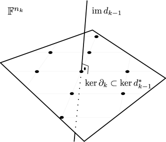
Figure 6. With the identifications 7.1, the space of $k$-forms becomes a direct sum of the image of $d_{k-1}$ and the kernel of its adjoint $d_{k-1}^{\ast}$, the latter of which contains the closed $k$-chains as a lattice.

Lemma 2.

Let $\omega\in\Omega^{k}(\mathcal{X},\mathbb{F})$, where $\mathbb{F}$ is a field of characteristic zero. Then

$$\omega\in\mathrm{im}\,d_{k-1}\Longleftrightarrow\langle\omega,c\rangle=0\textit{ for all }c\in\mathrm{ker}\,\partial_{k}.$$

Remark 6:

Note, that for boundary cycles the condition is nothing but the closedness of the form $\omega$. Thus Lemma 2 states that a closed form $\omega\in\Omega^{k}(\mathcal{X},\mathbb{F})$ is exact if and only if the integral over all homology classes $[c]\in\mathrm{H}_{k}(\mathcal{X},\mathbb{Z})$ vanishes.

Let $\mathfrak{G}$ be an abelian group. The sequence below will be referred to as the $k$-th fundamental sequence of forms with coefficients in $\mathfrak{G}$:

$$\Omega^{k-1}(\mathcal{X},\mathfrak{G})\xrightarrow{d_{k-1}}\Omega^{k}(\mathcal{X},\mathfrak{G})\xrightarrow{\Phi_{k}}\mathrm{Hom}(\mathrm{ker}\,\partial_{k},\mathfrak{G})\to 0,$$

where $\Phi_{k}$ denotes the restriction to the kernel of $\partial_{k}$, i.e. $\Phi_{k}(\omega):=\left.\omega\right|_{\ker\partial_{k}}$.

Combining Lemma 1 and Lemma 2 we obtain that the fundamental sequence with coefficients in a field $\mathbb{F}$ of characteristic zero is exact for all $k>1$. This serves as an anchor point. The exactness propagates under surjective group homomorphisms.

Lemma 3.

Let $\mathfrak{A}\xrightarrow{f}\mathfrak{B}\to 0$ be a an exact sequence of abelian groups. Then, if the $k$-th fundamental sequence of forms is exact with coefficients in $\mathfrak{A}$, so it is with coefficients in $\mathfrak{B}$.

Proof.

By Lemma 1 the restriction map $\Phi_{k}$ is surjective for every abelian group. It is left to check that $\mathrm{ker}\,\Phi_{k}=\mathrm{im}\,d_{k-1}$ with coefficients in $\mathfrak{B}$. Let $\Omega\in\Omega^{k}(\mathcal{X},\mathfrak{B})$ such that $\Phi_{k}(\Omega)=0$. Since $f\colon\mathfrak{A}\to\mathfrak{B}$ is surjective, there is a form $\Xi\in\Omega^{k}(\mathcal{X},\mathfrak{A})$ such that $\Omega=f\circ\Xi$. Since $0=\Phi_{k}(\Omega)=f\circ\Phi_{k}(\Xi)$, we obtain that $\Phi_{k}(\Xi)$ takes its values in $\ker f$. Since $\Phi_{k}$ is surjective for arbitrary groups, there is $\Theta\in\Omega^{k}(\mathcal{X},\ker f)$ such that $\Phi_{k}(\Xi)=\Phi_{k}(\Theta)$. Hence $\Phi_{k}(\Xi-\Theta)=0$. Thus there is a form $\xi\in\Omega^{k-1}(\mathcal{X},\mathfrak{A})$ such that $d_{k-1}\xi=\Xi-\Theta$. Now, let $\omega:=f\circ\xi\in\Omega^{k-1}(\mathcal{X},\mathfrak{B})$. Then

$$d_{k-1}\omega=d_{k-1}f\circ\xi=f\circ d_{k-1}\xi=f\circ(\Xi-\Theta)=f\circ\Xi=\Omega.$$

Hence $\mathrm{ker}\,\Phi_{k}=\mathrm{im}\,d_{k-1}$ and the sequence (with coefficients in $\mathfrak{B}$) is exact. ∎

Remark 7:

The map $f\colon\mathbb{C}\to\mathbb{C},\,z\mapsto\exp(2\pi\imath\,z)$ provides a surjective group homomorphism from $\mathbb{C}$ onto $\mathbb{C}_{\ast}$, and similarly from $\mathbb{R}$ onto $\mathbb{S}$. Hence the $k$-th fundamental sequence of forms is exact for coefficients in $\mathbb{C}_{\ast}$ and in the unit circle $\mathbb{S}$.

Remark 8:

The $k$-th fundamental sequence with coefficients in an abelian group $\mathfrak{G}$ is exact if and only if $\Omega^{k}(\mathcal{X},\mathfrak{G})/d\Omega^{k-1}(\mathcal{X},\mathfrak{G})\cong\mathrm{Hom}(\ker\partial_{k},\mathfrak{G})$. The isomorphism is induced by the restriction map $\Phi_{k}$.

The following corollary is a consequence of Remark 7. It nicely displays the fibration of the complex line bundles by their $\mathbb{C}_{\ast}$-curvature.

Corollary 1.

For $\mathfrak{G}=\mathbb{S},\,\mathbb{C}_{\ast}$ the following sequence is exact:

$$1\to\mathrm{H}^{1}(\mathcal{X},\mathfrak{G})\hookrightarrow\Omega^{1}(\mathcal{X},\mathfrak{G})/d\Omega^{0}(\mathcal{X},\mathfrak{G})\xrightarrow{d}\Omega^{2}(\mathcal{X},\mathfrak{G})\rightarrow\mathrm{Hom}(\mathrm{ker}\,\partial_{2},\mathfrak{G})\to 1.$$

Definition 7.

Let $\Omega^{\ast}\in\Omega^{k}(\mathcal{X},\mathbb{S})$. A real-valued form $\Omega\in\Omega^{2}(\mathcal{X},\mathbb{R})$ is called compatible with $\Omega^{\ast}$ if $\Omega^{\ast}=\exp\bigl{(}\imath\Omega\bigr{)}$. A discrete hermitian line bundle with curvature is a discrete hermitian line bundle $\mathrm{L}$ with connection equipped with a closed $2$-form compatible with the $\mathbb{S}$-curvature of $\mathrm{L}$.

For real-valued forms it is common to denote the natural pairing with the $k$-chains by an integral sign, i.e. for $\omega\in\Omega^{k}(\mathcal{X},\mathbb{R})$ and $c\in\mathrm{C}_{k}(\mathcal{X},\mathbb{Z})$ we write

$$\int_{c}\omega:=\langle\omega,c\rangle=\omega(c).$$

Theorem 6.

Let $\mathrm{L}$ be a discrete hermitian line bundle with curvature $\Omega$. Then $\Omega$ is integral, i.e.

$$\int_{c}\Omega\in 2\pi\,\mathbb{Z},\quad\textit{ for all }c\in\ker\partial_{2}.$$

Proof.

By definition the curvature form $\Omega$ satisfies $\exp\bigl{(}\imath\Omega\bigr{)}=d\omega$ for some connection form $\omega\in\Omega^{1}(\mathcal{X},\mathbb{S})$. Thus, if $c\in\ker\partial_{2}$,

$$\exp\bigl{(}\imath\!\!\int_{c}\Omega\bigr{)}=\langle\exp(\imath\Omega),c\rangle=\langle d\omega,c\rangle=\langle\omega,\partial c\rangle=1.$$

This proves the claim. ∎

Conversely, Corollary 1 yields a discrete version of a theorem of André Weil ([19, 11]), which states that any closed smooth integral $2$-form on a manifold $\mathrm{M}$ can be realized as the curvature of a hermitian line bundle. This plays a prominent role in the process of prequantization [18].

Theorem 7.

If $\Omega\in\Omega^{2}(\mathcal{X},\mathbb{R})$ is integral, then there exists a hermitian line bundle with curvature $\Omega$.

Proof.

Consider $\Omega^{\ast}:=\exp(i\Omega)$. Since $\Omega$ is integral, $\langle\Omega^{\ast},c\rangle=1$ for all $c\in\mathrm{ker}\,\partial_{2}$. By Corollary 1, there exists $r\in\Omega^{1}(\mathcal{X},\mathbb{S})$ such that $dr=\Omega^{\ast}$. This in turn defines a hermitian line bundle with curvature $\Omega$. ∎

Remark 9:

Moreover, Corollary 1 shows that the connections of two such bundles differ by an element of $\mathrm{H}^{1}(\mathcal{X},\mathbb{S})$. Thus the space of discrete hermitian line bundles with fixed curvature $\Omega$ can be parameterized by $\mathrm{H}^{1}(\mathcal{X},\mathbb{S})$.

8. The Index Formula for Hermitian Line Bundles

Before we define the degree of a discrete hermitian line bundle with curvature or the index form of a section, let us first recall the situation in the smooth setting. Therefore, let $\mathrm{L}\to\mathrm{M}$ be a smooth hermitian line bundle with connection. Since the curvature tensor $R^{\nabla}$ of $\nabla$ is a $2$-form taking values in the skew-symmetric endomorphisms of $\mathrm{L}$, it is completely described by a closed real-valued $2$-form $\Omega\in\Omega^{2}(\mathrm{M},\mathbb{R})$,

$$R^{\nabla}=-\imath\Omega.$$

The following theorem shows an interesting relation between the index sum of a section $\psi\in\Gamma(\mathrm{L})$, the curvature $2$-form $\Omega$, and the rotation form $\xi^{\psi}$ of $\psi$. This form is defined as follows:

$$\xi^{\psi}:=\frac{\langle\nabla\psi,\imath\psi\rangle}{\langle\psi,\psi\rangle}.$$

Theorem 8.

Let $\mathrm{L}\to\mathrm{M}$ be a smooth hermitian line bundle with connection and $\Omega$ its curvature $2$-form. Let $\psi\in\Gamma(\mathrm{L})$ be a section with a discrete zero set $Z$. Then, if $C$ is a finite smooth $2$-chain such that $\partial C\mathop{\cap}Z=\emptyset$,

$$2\pi\sum_{p\in{C\mathop{\cap}Z}}\mathrm{ind}_{p}^{\psi}=\int_{\partial C}\xi^{\psi}+\int_{C}\Omega.$$

Proof.

We can assume that $C$ is a single smooth triangle. Then we can express $\psi$ on $C$ in terms of a complex-valued function $z$ and a pointwise-normalized local section $\phi$, i.e. $\psi=z\,\phi$. Since $\mathrm{Im}(\tfrac{dz}{z})=d\,\mathrm{arg}(z)$, we obtain

$$\xi^{\psi}=\frac{1}{|z|^{2}}\langle dz\,\phi+z\,\nabla\phi,\imath z\,\phi\rangle=\langle\frac{dz}{z}\,\phi,\imath\phi\rangle+\langle\nabla\phi,\imath\phi\rangle=d\,\mathrm{arg}(z)+\langle\nabla\phi,\imath\phi\rangle.$$

Moreover, away from zeros, we have

$$d\langle\nabla\phi,\imath\phi\rangle=\langle R^{\nabla}\phi,\imath\phi\rangle+\langle\nabla\phi\wedge\imath\nabla\phi\rangle=\langle R^{\nabla}\phi,\imath\phi\rangle=-\Omega.$$

Hence we obtain

$$\int_{\partial C}\xi^{\psi}=\int_{\partial C}d\,\mathrm{arg}(z)+\int_{\partial C}\langle\nabla\phi,\imath\phi\rangle=2\pi\sum_{p\in{C\mathop{\cap}Z}}\mathrm{index}_{p}(\psi)-\int_{C}\Omega.$$

This proves the claim. ∎

In the case that $\mathrm{L}$ is a hermitian line bundle with connection over a closed oriented surface $\mathrm{M}$, Theorem 8 tells us that $\int_{\mathrm{M}}\Omega\in 2\pi\mathbb{Z}$. This yields a well-known topological invariant - the degree of $\mathrm{L}$:

$$\mathrm{deg}\bigl{(}\mathrm{L}\bigr{)}:=\frac{1}{2\pi}\int_{\mathrm{M}}\Omega.$$

From Theorem 8 we immediately obtain the famous Poincaré-Hopf index theorem.

Theorem 9.

Let $\mathrm{L}\to\mathrm{M}$ be a smooth hermitian line bundle over a closed oriented surface. Then, if $\psi\in\Gamma(\mathrm{L})$ is a section with isolated zeros,

$$\mathrm{deg}\bigl{(}\mathrm{L}\bigr{)}=\sum_{p\in\mathrm{M}}\mathrm{ind}^{\psi}_{p}.$$

Now, let us consider the discrete case. In general, a section of a discrete vector bundle $\mathrm{E}\to\mathcal{X}$ with vertex set $\mathcal{V}$ is a map $\psi\colon\mathcal{V}\to\mathrm{E}$ such that the following diagram commutes

,

i.e. $\pi\circ\psi=id$. As in the smooth case, the space of sections of $\mathrm{E}$ is denoted by $\Gamma(\mathrm{E})$.

Now, let $\mathrm{L}\to\mathcal{X}$ be a discrete hermitian line bundle with curvature $\Omega$ and let $\psi\in\Gamma(\mathrm{L})$ be a nowhere-vanishing section such that

(8.1) $$\eta_{\ij}(\psi_{i})\neq-\psi_{j}$$

for each edge $\ij$ of $\mathcal{X}$. Here $\eta$ denotes the connection of $\mathrm{L}$ as usual. The rotation form $\xi^{\psi}$ of $\psi$ is then defined as follows:

$$\xi^{\psi}_{\ij}:=\arg\bigl{(}\frac{\psi_{j}}{\eta_{\ij}(\psi_{i})}\bigr{)}\in(-\pi,\pi).$$

Remark 10:

Equation (8.1) can be interpreted as the condition that no zero lies in the $1$-skeleton of $\mathcal{X}$ (compare Section 11). Actually, given a consistent choice of the argument on each oriented edge, we could drop this condition. Figuratively speaking, if a section has a zero in the $1$-skeleton, then we decide whether we push it to the left or the right face of the edge.

Now we can define the index form of a discrete section:

Definition 8.

Let $\mathrm{L}\to\mathcal{X}$ be a discrete hermitian line bundle with curvature $\Omega$. For $\psi\in\Gamma(\mathrm{L})$, we define the index form of $\psi$ by

$$\mathrm{ind}^{\psi}:=\frac{1}{2\pi}\bigl{(}d\xi^{\psi}+\Omega\bigr{)}.$$

Theorem 10.

The index form of a nowhere-vanishing discrete section is $\mathbb{Z}$-valued.

Proof.

Let $\mathrm{L}$ be a discrete hermitian line bundle with curvature and let $\eta$ be its connection. Let $\psi\in\Gamma(\mathrm{L})$ be a nowhere-vanishing section. Now, choose a connection form $\omega$, i.e. $\eta=\omega\beta$, where $\beta$ is a trivial connection on $\mathrm{L}$. Then we can write $\psi$ with respect to a non-vanishing parallel section $\phi$ of $\beta$, i.e. there is a $\mathbb{C}$-valued function $z$ such that $\psi=z\phi$. Then $\xi^{\psi}_{\ij}=\arg\bigl{(}\frac{z_{j}}{\omega_{\ij}z_{i}}\bigr{)}$ and thus

$$\exp\bigl{(}2\pi\imath\,d\xi^{\psi}_{ijk}\bigr{)}=\exp\bigl{(}\imath\,\arg\bigl{(}\frac{z_{i}}{\omega_{ki}z_{k}}\bigr{)}+\imath\,\arg\bigl{(}\frac{z_{j}}{\omega_{\ij}z_{i}}\bigr{)}+\imath\,\arg\bigl{(}\frac{z_{k}}{\omega_{jk}z_{j}}\bigr{)}\bigr{)}=\frac{1}{d\omega_{ijk}}.$$

Thus

$$\exp\bigl{(}2\pi\imath\,\mathrm{ind}^{\psi}_{ijk}\bigr{)}=\frac{\exp\bigl{(}\imath\Omega_{ijk}\bigr{)}}{d\omega_{ijk}}=1.$$

This proves the claim. ∎

If $\mathrm{L}$ is a discrete hermitian line bundle with curvature $\Omega$ over a closed oriented surface $\mathcal{X}$, then we define the degree of $\mathrm{L}$ just as in the smooth case:

$$\mathrm{deg}\bigl{(}\mathrm{L}\bigr{)}:=\frac{1}{2\pi}\int_{\mathcal{X}}\Omega.$$

Here we have identified $\mathcal{X}$ by the corresponding closed $2$-chain. From Theorem 6 we obtain the following corollary.

Corollary 2.

The degree of a discrete hermitian line bundle with curvature is an integer:

$$\mathrm{deg}\bigl{(}\mathrm{L}\bigr{)}\in\mathbb{Z}.$$

The discrete Poincaré-Hopf index theorem follows easily from the definitions:

Theorem 11.

Let $\mathrm{L}\to\mathcal{X}$ be a discrete hermitian line bundle with curvature $\Omega$ over an oriented simplicial surface. If $\psi\in\Gamma(\mathrm{L})$ is a non-vanishing discrete section, then

$$\mathrm{deg}\bigl{(}\mathrm{L}\bigr{)}=\sum_{ijk\in\mathcal{X}}\mathrm{ind}^{\psi}_{ijk}.$$

Proof.

Since the integral of an exact form over a closed oriented surface vanishes,

$$2\pi\,\mathrm{deg}\bigl{(}\mathrm{L}\bigr{)}=\int_{\mathcal{X}}\Omega=\int_{\mathcal{X}}d\xi^{\psi}+\Omega=2\pi\,\sum_{ijk\in\mathcal{X}}\mathrm{ind}^{\psi}_{ijk},$$

as was claimed. ∎

9. Piecewise-Smooth Vector Bundles over Simplicial Complexes

It is well-known that each abstract simplicial complex $\mathcal{X}$ has a geometric realization which is unique up to simplicial isomorphism. In particular, each abstract simplex is realized as an affine simplex. Moreover, each face $\sigma^{\prime}$ of a simplex $\sigma\in\mathcal{X}$ comes with an affine embedding

$$\iota_{\sigma^{\prime}\!\sigma}\colon\sigma^{\prime}\hookrightarrow\sigma.$$

In the following, we will not distinguish between the abstract simplicial complex and its geometric realization.

Definition 9.

A piecewise-smooth vector bundle $\mathrm{E}$ over a simplicial complex $\mathcal{X}$ is a topological vector bundle $\pi\colon\mathrm{E}\to\mathcal{X}$ such that

1. for each $\sigma\in\mathcal{X}$ the restriction $\mathrm{E}_{\sigma}:=\left.\mathrm{E}\right|_{\sigma}$ is a smooth vector bundle over $\sigma$,

2. for each face $\sigma^{\prime}$ of $\sigma\in\mathcal{X}$, the inclusion $\mathrm{E}_{\sigma^{\prime}}\hookrightarrow\mathrm{E}_{\sigma}$ is a smooth embedding.

As a simplicial complex, $\mathcal{X}$ has no tangent bundle. Nonetheless, differential forms survive as collections of smooth differential forms defined on the simplices which are compatible in the sense that they agree on common faces:

Definition 10.

Let $\mathrm{E}$ be a piecewise-smooth vector bundle over $\mathcal{X}$. An $\mathrm{E}$-valued differential $k$-form is a collection $\omega=\{\omega_{\sigma}\in\Omega^{k}(\sigma,\mathrm{E}_{\sigma})\}_{\sigma\in\mathcal{X}}$ such that for each face $\sigma^{\prime}$ of a simplex $\sigma\in\mathcal{X}$ the following relation holds:

$$\iota_{\sigma^{\prime}\!\sigma}^{\ast}\omega_{\sigma}=\omega_{\sigma^{\prime}},$$

where $\iota_{\sigma^{\prime}\!\sigma}\colon\sigma^{\prime}\hookrightarrow\sigma$ denotes the inclusion. The space of $\mathrm{E}$-valued differential $k$-forms is denoted by $\Omega_{ps}^{k}(\mathcal{X},\mathrm{E})$.

Remark 11:

Note that a $0$-form defines a continuous map on the simplicial complex. Hence the definition includes functions and, more generally, sections: A piecewise-smooth section of $\mathrm{E}$ is a continuous section $\psi\colon\mathcal{X}\to\mathrm{E}$ such that for each simplex $\sigma\in\mathcal{X}$ the restriction $\psi_{\sigma}:=\left.\psi\right|_{\sigma}\colon\sigma\to\mathrm{E}_{\sigma}$ is smooth, i.e.

$$\Gamma_{ps}(\mathrm{E}):=\bigl{\{}\psi\colon\mathcal{X}\to\mathrm{E}\mid\psi_{\sigma}\in\Gamma(\mathrm{E}_{\sigma})\textit{ for all }\sigma\in\mathcal{X}\bigr{\}}.$$

Since the pullback commutes with the wedge-product $\wedge$ and the exterior derivative $d$ of real-valued forms, we can define the wedge product and the exterior derivative of piecewise-smooth differential forms by applying it componentwise.

Definition 11.

For $\omega=\{\omega_{\sigma}\}_{\sigma\in\mathcal{X}}\in\Omega_{ps}^{k}(\mathcal{X},\mathbb{R}),\,\eta=\{\eta_{\sigma}\}_{\sigma\in\mathcal{X}}\in\Omega_{ps}^{\ell}(\mathcal{X},\mathbb{R})$,

$$\omega\wedge\eta:=\{\omega_{\sigma}\wedge\eta_{\sigma}\}_{\sigma\in\mathcal{X}},\quad d\omega:=\{d\omega_{\sigma}\}_{\sigma\in\mathcal{X}}.$$

All the standard properties of $\wedge$ and $d$ also hold in the piecewise-smooth case.

Definition 12.

A connection on a piecewise-smooth vector bundle $\mathrm{E}$ over $\mathcal{X}$ is a linear map $\nabla\colon\Gamma_{ps}(\mathrm{E})\to\Omega_{ps}^{1}(\mathcal{X},\mathrm{E})$ such that

$$\nabla(f\psi)=df\,\psi+f\,\nabla\psi,\quad\textit{for all }f\in\Omega_{ps}^{0}(\mathcal{X},\mathbb{R}),\,\psi\in\Gamma_{ps}(\mathrm{E}).$$

Once we have a connection on a smooth vector bundle we obtain a corresponding exterior derivative $d^{\nabla}$ on $\mathrm{E}$-valued forms.

Theorem 12.

Let $\mathrm{E}$ be a piecewise-smooth vector bundle over $\mathcal{X}$. Then there is a unique linear map $d^{\nabla}\colon\Omega_{ps}^{k}(\mathcal{X},\mathrm{E})\to\Omega_{ps}^{k+1}(\mathcal{X},\mathrm{E})$ such that $d^{\nabla}\psi=\nabla\psi$ for all $\psi\in\Gamma_{ps}(\mathrm{E})$ and

$$d^{\nabla}(\omega\wedge\eta)=d\omega\wedge\eta+(-1)^{k}\omega\wedge d^{\nabla}\eta$$

for all $\omega\in\Omega_{ps}^{k}(\mathcal{X},\mathbb{R})$ and $\eta\in\Omega_{ps}^{\ell}(\mathcal{X},\mathrm{E})$.

The curvature tensor survives as a piecewise-smooth $\mathrm{End}(\mathrm{E})$-valued $2$-form:

Definition 13.

Let $\mathrm{E}\to\mathcal{X}$ be a piecewise-smooth vector bundle. The endomorphism-valued curvature $2$-form of a connection $\nabla$ on $\mathrm{E}$ is defined as follows:

$$d^{\nabla}\circ d^{\nabla}\in\Omega_{ps}^{2}(\mathcal{X},\mathrm{End}(\mathrm{E})).$$

10. The Associated Piecewise-Smooth Hermitian Line Bundle

Let $\tilde{\mathrm{L}}\to\mathcal{X}$ be a piecewise-smooth hermitian line bundle with connection $\nabla$ over a simplicial complex. Just as in the smooth case the endomorphism-valued curvature $2$-form takes values in the skew-adjoint endomorphisms and hence is given by a piecewise-smooth real-valued $2$-form $\tilde{\Omega}$:

$$d^{\nabla}\circ d^{\nabla}=-\imath\tilde{\Omega}.$$

Since each simplex of $\mathcal{X}$ has an affine structure, we can speak of piecewise-constant forms.

The goal of this section will be to construct for each discrete hermitian line bundle with curvature a piecewise-smooth hermitian line bundle with piecewise-constant curvature which in a certain sense naturally contains the discrete bundle. We first prove two lemmata.

Lemma 4.

To each closed discrete real-valued $k$-form $\omega$ there corresponds a unique piecewise-constant piecewise-smooth $k$-form $\tilde{\omega}$ such that

$$\omega(c)=\int_{c}\tilde{\omega},\quad\textit{ for all }c\in\mathrm{C}_{k}(\mathcal{X},\mathbb{Z}).$$

The form $\tilde{\omega}$ will be called the piecewise-smooth form associated to $\omega$.

Proof.

It is enough to consider just a single $n$-simplex $\sigma$. We denote the space of piecewise-constant piecewise-smooth $k$-forms on $\sigma$ by $\Omega^{k}_{c}$ and the space of discrete $k$-forms on $\sigma$ by $\Omega^{k}_{d}$. Consider the linear map $F\colon\Omega^{k}_{c}\to\Omega^{k}_{d}$ that assigns to $\tilde{\omega}\in\Omega^{k}_{c}$ the discrete $k$-form given by

$$F(\tilde{\omega})_{\sigma^{\prime}}:=\int_{\sigma^{\prime}}\tilde{\omega}.$$

Clearly, $F$ is injective. Moreover, since each piecewise-constant piecewise-smooth form is closed, we have $\mathrm{im}\,\,F\subset\ker d_{k}$, where $d_{k}$ denotes the discrete exterior derivative. Hence it is enough to show that the space of closed discrete $k$-forms on $\sigma$ is of dimension $\binom{n}{k}$. This we do by induction. Clearly, $\dim\ker d_{0}=1=\binom{n}{0}$. Now suppose that $\dim\ker d_{k-1}=\binom{n}{k-1}$. By Lemma 2, we have $\ker d_{k}=\mathrm{im}\,d_{k-1}$. Hence

$$\dim\ker d_{k}=\dim\mathrm{im}\,d_{k-1}=\dim\Omega^{k}_{d}-\dim\ker d_{k-1}=\tbinom{n+1}{k}-\tbinom{n}{k-1}=\tbinom{n}{k}.$$

Therefore, for each closed discrete $k$-form we obtain a unique piecewise-constant piecewise-smooth $k$-form which has the desired integrals on the $k$-simplices. ∎

It is a classical result that on star-shaped domains $U\subset\mathbb{R}^{N}$ each closed form is exact: If $\Omega\in\Omega^{k}(U,\mathbb{R})$ is closed, then there exists a form $\omega\in\Omega^{k-1}(U,\mathbb{R})$ such that $\Omega=d\omega$. Moreover, the potential can be constructed explicitly by the map $K\colon\Omega^{k}(U,\mathbb{R})\to\Omega^{k-1}(U,\mathbb{R})$ given by

$$K(\Omega)=\sum_{i_{1}<\cdots<i_{k}}\sum_{\alpha=1}^{k}(-1)^{\alpha-1}\Bigl{(}\int_{0}^{1}t^{k-1}\Omega_{i_{1}\cdots i_{k}}(tx)dt\Bigr{)}\,x_{i_{\alpha}}\,dx_{i_{1}}\wedge\ldots\wedge\widehat{dx_{i_{\alpha}}}\wedge\ldots\wedge dx_{i_{k}},$$

where $\Omega=\sum_{i_{1}<\cdots<i_{k}}\Omega_{i_{1}\cdots i_{k}}\,dx_{i_{1}}\wedge\ldots\wedge dx_{i_{k}}$. One directly can check that

$$K(d\Omega)+d\,K(\Omega)=\Omega.$$

Hence, if $d\Omega=0$, we get $\Omega=d\,K(\Omega)$. The same construction works for piecewise-smooth forms defined on the star of a simplex. This yields the following piecewise-smooth version of the Poincaré-Lemma.

Lemma 5.

On the star of a simplex each closed piecewise-smooth form is exact.

Now we are ready to prove the main result of this section.

Theorem 13.

Let $\mathrm{L}\to\mathcal{X}$ be a discrete hermitian line bundle with curvature $\Omega$ over a simplicial complex and let $\tilde{\Omega}$ be the piecewise-smooth $2$-form associated to $\Omega$. Then there is a piecewise-smooth hermitian line bundle $\tilde{\mathrm{L}}\to\mathcal{X}$ with connection $\tilde{\nabla}$ of curvature $\tilde{\Omega}$ such that $\tilde{\mathrm{L}}_{i}=\mathrm{L}_{i}$ for each vertex $i$ and the parallel transports coincide along each edge path. The bundle $\tilde{\mathrm{L}}$ is unique up to isomorphism.

Proof.

First we construct the piecewise-smooth hermitian line bundle. Let $\mathrm{L}\to\mathcal{X}$ be a discrete hermitian line bundle with curvature $\Omega$ and let $\eta$ denote its connection. Let $\mathcal{V}$ be the vertex set of $\mathcal{X}$ and let $S_{i}$ denote the open vertex star of the vertex $i$. Further, since $\Omega$ is closed, by Lemma 4, there is a piecewise-constant piecewise-smooth form $\tilde{\Omega}$ associated to $\Omega$. Now, consider the set

$$\hat{\mathrm{L}}:=\mathop{\sqcup}_{i\in\mathcal{V}}S_{i}\times\mathrm{L}_{i}.$$

Note, that $S_{i}\mathop{\cap}S_{j}\neq\emptyset$ if and only if $\ij$ is an edge of $\mathcal{X}$ or $i=j$. Thus, if we set $\eta_{ii}:=\left.\mathrm{id}\right|_{\mathrm{L}_{i}}$, we can define an equivalence relation on $\hat{\mathrm{L}}$ as follows:

$$(i,p,u)\sim(j,q,v):\Longleftrightarrow p=q\textit{ and }v=\exp\bigl{(}-\imath\int_{\Delta_{\ij}^{p}}\tilde{\Omega}\bigr{)}\eta_{\ij}(u),$$

where $\Delta_{\ij}^{p}$ denotes the oriented triangle spanned by the point $i,j$ and $p$. Note here that $\Delta_{\ij}^{p}$ is completely contained in some simplex of $\mathcal{X}$. Let us check shortly that this really defines an equivalence relation. Here the only non-trivial property is transitivity. Therefore, let $(i,p,u)\sim(j,q,v)$ and $(j,q,v)\sim(k,r,w)$. Thus we have $p=q=r$ and $p$ lies in a simplex which contains the oriented triangle $ijk$. Clearly, the $2$-chain $\Delta_{\ij}^{p}+\Delta_{jk}^{p}+\Delta_{ki}^{p}$ is homologous to $ijk$ and since piecewise-constant forms are closed we get

$$\int_{\Delta_{\ij}^{p}+\Delta_{jk}^{p}}\tilde{\Omega}=-\int_{\Delta_{ki}^{p}}\tilde{\Omega}+\int_{ijk}\tilde{\Omega}=\int_{\Delta_{ik}^{p}}\tilde{\Omega}+\Omega_{ijk}.$$

Hence we obtain

$$w =\exp\bigl{(}-\imath\int_{\Delta_{jk}^{p}}\tilde{\Omega}\bigr{)}\eta_{jk}\Bigl{(}\exp\bigl{(}-\imath\int_{\Delta_{\ij}^{p}}\tilde{\Omega}\bigr{)}\eta_{\ij}(u)\Bigr{)}$$

$$=\exp\bigl{(}-\imath\int_{\Delta_{\ij}^{p}+\Delta_{jk}^{p}}\tilde{\Omega}\bigr{)}\eta_{jk}\circ\eta_{\ij}(u)$$

$$=\exp\bigl{(}-\imath\int_{\Delta_{ik}^{p}}\tilde{\Omega}-\imath\Omega_{ijk}\bigr{)}\eta_{jk}\circ\eta_{\ij}(u)$$

$$=\exp\bigl{(}-\imath\int_{\Delta_{ik}^{p}}\tilde{\Omega}\bigr{)}\eta_{ik}(u),$$

and thus $(i,p,u)\sim(k,r,w)$. Hence $\sim$ defines an equivalence relation. One can check now that the quotient $\tilde{\mathrm{L}}:=\hat{\mathrm{L}}/_{\sim}$ is a piecewise-smooth line bundle over $\mathcal{X}$. The local trivializations are then basically given by the inclusions $S_{i}\times\mathrm{L}_{i}\hookrightarrow\tilde{\mathrm{L}}$ sending a point to the corresponding equivalence class. Moreover, all transition maps are unitary so that the hermitian metric of $\mathrm{L}$ extends to $\tilde{\mathrm{L}}$ and turns $\tilde{\mathrm{L}}$ into a hermitian line bundle. Clearly, $\left.\tilde{\mathrm{L}}\right|_{\mathcal{V}}=\mathrm{L}$.

Next, we need to construct the connection. Therefore we will use an explicit system of local sections: Choose for each vertex $i\in\mathcal{V}$ a unit vector $X_{i}\in\mathrm{L}_{i}$ and define $\phi_{i}(p):=[i,p,X_{i}]$. This yields for each vertex $i$ a piecewise-smooth section $\phi_{i}$ define on the star $S_{i}$. For each non-empty intersection $S_{i}\mathop{\cap}S_{j}\not=\emptyset$ we then obtain a function $g_{\ij}\colon S_{i}\mathop{\cap}S_{j}\to\mathbb{S}$. By the above construction, we find that, if $\eta_{\ij}(X_{i})=r_{\ij}X_{j}$,

(10.1) $$g_{\ij}(p)=r_{\ij}\exp\bigl{(}-\imath\int_{\Delta_{\ij}^{p}}\tilde{\Omega}\bigr{)}.$$

Since $\tilde{\Omega}$ is closed, Lemma 5 tells us that $\tilde{\Omega}|_{S_{i}}$ is exact. Hence there is a piecewise-smooth $1$-form $\omega_{i}$ defined on $S_{i}$ such that $d\omega_{i}=\tilde{\Omega}|_{S_{i}}$. In general, the form $\omega_{i}$ is only unique up to addition of an exact $1$-form, but among those there is a unique form $\omega_{i}$ which is zero along the radial directions originating from $i$. To see this, just choose some potential $\tilde{\omega}_{i}$ of $\Omega|_{S_{i}}$ and define a function $f\colon S_{i}\to\mathbb{R}$ as follows:

For $p\in S_{i}$, let $f(p):=\int_{\gamma_{i}^{\,p}}\tilde{\omega}_{i}$, where $\gamma_{i}^{\,p}$ denote the linear path from the vertex $i$ to the point $p$. Then $\omega_{i}:=\tilde{\omega}_{i}-df$ is a piecewise-smooth potential of $\left.\Omega\right|_{S_{i}}$ and vanishes on radial directions. For the uniqueness, let $\hat{\omega}_{i}$ be another such potential. Then, the difference $\omega_{i}-\hat{\omega}_{i}$ is closed and hence exact on $S_{i}$, i.e. there is $f\colon S_{i}\to\mathbb{R}$ such that $df=\omega_{i}-\hat{\omega}_{i}$. Since $df$ vanishes on radial directions $f$ is constant on radial lines starting at $i$ and hence constant on $S_{i}$. Thus $\omega_{i}=\hat{\omega}_{i}$.

Suppose that for each edge $\ij$ the forms $\omega_{i}$ and $\omega_{j}$ are compatible, i.e., wherever both are defined,

$$\imath\omega_{j}=\imath\omega_{i}+d\log g_{\ij}.$$

Then we can define a connection $\nabla$ as follows: Let $\psi\in\Gamma\bigl{(}\tilde{\mathrm{L}}\bigr{)}$ and let $X\in\mathrm{T}_{p}\sigma$ for some simplex $\sigma$ of $\mathcal{X}$, then there is some $S_{i}\ni p$. On $S_{i}$ we can express $\psi$ with respect to $\phi_{i}$, i.e. $\psi=z\,\phi_{i}$ for some piecewise-smooth function $z\colon S_{i}\to\mathbb{C}$. Then we define

(10.2) $$\nabla_{X}\psi:=\bigl{(}dz(X)-\imath\omega_{i}(X)z\bigr{)}\phi_{i}.$$

In general there are several stars that contain the point $p$. From compatibility easily follows that the definition does not depend on the choice of the vertex. Hence we have constructed a piecewise smooth connection $\nabla$. One easily checks that $\nabla$ is unitary and since $d\omega_{i}=\tilde{\Omega}|_{S_{i}}$ we get $d^{\nabla}\circ d^{\nabla}=-\imath\tilde{\Omega}$ as desired.

So it is left to check the compatibility of the forms $\omega_{\ij}$ constructed above. Let $\ij$ be some edge and let $p_{0}$ be a point in its interior. Since $\omega_{i}-\omega_{j}$ is closed, we can define $\varphi\colon S_{i}\mathop{\cap}S_{j}\to\mathbb{R}$ by $\varphi(p):=\int_{\gamma_{p}}\omega_{i}-\omega_{j}$, where $\gamma_{p}$ is some path in $S_{i}\mathop{\cap}S_{j}$ from the point $p_{0}$ to the point $p$. Then, for $p\in S_{i}\mathop{\cap}S_{j}$,

$$\int_{\Delta_{p}}\Omega=\int_{\partial\Delta_{p}}\omega_{j}=\int_{\ij+\gamma_{j}^{\,p}-\gamma_{i}^{\,p}}\omega_{j}=-\int_{\gamma_{i}^{\,p}}\omega_{j}=\int_{\gamma_{i}^{\,p}}\omega_{i}-\omega_{j}=\varphi(p),$$

where as above $\gamma_{i}^{\,p}$ denotes the linear path from $i$ to $p$ and, similarly, $\gamma_{j}^{\,p}$ denotes the linear path from $j$ to the point $p$. From this we obtain

$$\omega_{i}-\omega_{j}=d\varphi=d\int_{\Delta_{p}}\Omega$$

and in particular $\imath\omega_{j}=\imath\omega_{i}+d\log g_{\ij}$. This shows the existence.

Now suppose there are two such piecewise-smooth bundles $\tilde{\mathrm{L}}$ and $\hat{\mathrm{L}}$ with connection $\tilde{\nabla}$ and $\hat{\nabla}$, respectively. We want to construct an isomorphism between $\tilde{\mathrm{L}}$ and $\hat{\mathrm{L}}$. Therefore we again use local systems. Explicitly, we choose a discrete direction field $X\in\mathrm{L}$. This yields for each vertex $i$ a vector $X_{i}\in\tilde{\mathrm{L}}_{i}=\hat{\mathrm{L}}_{i}$ which extends by parallel transport along rays starting at $i$ to a local sections $\tilde{\phi}_{i}$ of $\tilde{\mathrm{L}}$ and, similarly, to a local section $\hat{\phi}_{i}$ of $\hat{\mathrm{L}}$ defined on $S_{i}$.

Now we define $F\colon\tilde{\mathrm{L}}\to\hat{\mathrm{L}}$ to be unique map which is linear on the fibers and satisfies $F(\tilde{\phi}_{i})=\hat{\phi}_{i}$ on $S_{i}$. To see that $F$ is well-defined, we need to check that it is compatible with the transition maps. But by construction both systems have equal transition maps, namely the the functions $g_{\ij}$ from Equation (10.1) with $r_{\ij}$ given by $\eta_{\ij}(X_{i})=r_{\ij}X_{j}$. Now, if $z_{i}\,\tilde{\phi}_{i}=z_{j}\,\tilde{\phi}_{j}$, then $z_{i}=z_{j}\,g_{\ij}$ and hence

$$F(z_{i}\tilde{\phi}_{i})=z_{i}\,\hat{\phi}_{i}=z_{i}\,g_{\ij}\hat{\phi}_{j}=z_{j}\,\hat{\phi}_{j}=F(z_{j}\,\tilde{\phi}_{j}).$$

Using Equation (10.2) one similarly shows that $F\circ\tilde{\nabla}=\hat{\nabla}\circ F$. Thus $\tilde{\mathrm{L}}\cong\hat{\mathrm{L}}$. ∎

11. Finite Elements for Hermitian Line Bundles With Curvature

In this section we want to present a specific finite element space on the associated piecewise-smooth hermitian line bundle of a discrete hermitian line with curvature. They are constructed from the local systems that played such a prominent role in the proof of Theorem 13 and the usual piecewise-linear hat function.

Let $\tilde{\mathrm{L}}$ be the associated piecewise-smooth bundle of a discrete hermitian line bundle $\mathrm{L}\to\mathcal{X}$ and let $x_{i}\colon\mathcal{X}\to\mathbb{R}$ denote the barycentric coordinate of the vertex $i\in\mathcal{V}$, i.e. the unique piecewise-linear function such that $x_{i}(j)=\delta_{\ij}$, where $\delta$ is the Kronecker delta. Clearly,

$$\Gamma(\mathrm{L})=\mathop{\bigoplus}_{i\in\mathcal{V}}\mathrm{L}_{i}.$$

To each $X\in\mathrm{L}_{i}$ we now construct a piecewise-smooth section $\tilde{\psi}$ as follows: First, we extend $X$ to the vertex star $S_{i}$ of the vertex $i$ using the parallel transport along rays starting at $i$. To get a global section $\tilde{\psi}\in\Gamma_{ps}(\mathrm{L})$ we use $x_{i}$ to scale $\tilde{\phi}$ down to zero on $\partial S_{i}$ and extend it by zero to $\mathcal{X}$, i.e.

$$\tilde{\psi}_{p}:=\begin{cases}\hfill x_{i}(p)\tilde{\phi}_{p}\hfill&\textit{ for }p\in S_{i},\\ \hfill 0\hfill&\textit{ else.}\end{cases}$$

The above construction yields a linear map $\iota\colon\Gamma(\mathrm{L})\to\Gamma_{ps}(\tilde{\mathrm{L}})$. Clearly, $\iota$ is injective - a left-inverse is just given by the restriction map

$$\Gamma_{ps}(\tilde{\mathrm{L}})\ni\tilde{\psi}\mapsto\bigl{.}\tilde{\psi}\bigr{|}_{\mathcal{V}}\in\Gamma(\mathrm{L}).$$

Definition 14.

The space of piecewise-linear sections is given by $\Gamma_{pl}(\tilde{\mathrm{L}}):=\mathrm{im}\,\iota$.

Thus we identified each section of a discrete hermitian line bundle with curvature with a piecewise-linear section of the associated piecewise-smooth bundle. This allows to define a discrete hermitian inner product and a discrete Dirichlet energy on $\Gamma(\mathrm{L})$, which is a generalization of the well-known cotangent Laplace operator for discrete functions on triangulated surfaces. Before we come to the Dirichlet energy, we define Euclidean simplicial complexes.

Similarly to piecewise-smooth forms we can define piecewise-smooth (contravariant) $k$-tensors as collections of compatible $k$-tensors: A piecewise-smooth $k$-tensor is a collection $T=\{T_{\sigma}\}_{\sigma\in\mathcal{X}}$ of smooth contravariant $k$-tensors $T_{\sigma}$ on $\sigma$ such that

$$\iota_{\sigma^{\prime}\sigma}^{\ast}T_{\sigma}=T_{\sigma^{\prime}},$$

whenever $\sigma^{\prime}$ is a face of $\sigma$. A Riemannian simplicial complex is then a simplicial complex $\mathcal{X}$ equipped with a piecewise-smooth Riemannian metric, i.e. a piecewise-smooth positive-definite symmetric $2$-tensor $g$ on $\mathcal{X}$.

The following lemma tells us that the space of constant piecewise-smooth symmetric tensors is isomorphic to functions on $1$-simplices.

Lemma 6.

Let $\mathcal{X}$ be a simplicial complex and let $\mathcal{E}$ denote the set of its $1$-simplices. For each function $f\colon\mathcal{E}\to\mathbb{R}$ there exists a unique constant piecewise-smooth symmetric $2$-tensor $S$ such that for each $1$-simplex $e=\{i,j\}$

$$S_{e}(j-i,j-i)=f(e).$$

Proof.

It is enough to consider a single affine $n$-simplex $\sigma=\{i_{0},\ldots,i_{n}\}$ with vector space $V$. Consider the map $F$ that sends a symmetric $2$-tensor $S$ on $V$ to the function given by

$$F(S)(e):=S(i_{k}-i_{j},i_{k}-i_{j}),\quad e=\{i_{j},i_{k}\}\subset\sigma.$$

Clearly, $F$ is linear. Moreover, if $Q$ denotes the quadratic form corresponding to $S$, i.e. $Q(X):=S(X,X)$, then

$$S(X,Y)=\tfrac{1}{2}\bigl{(}Q(X)+Q(Y)-Q(X-Y)\bigr{)}.$$

Hence, from $F(S)=0$ follows $S=0$. Thus $F$ is injective. Clearly, the space of symmetric bilinear forms is of dimension $n(n+1)/2$, which equals the number of $1$-simplices. Thus $F$ is an isomorphism. This proves the claim. ∎

It is also easy to write down the corresponding symmetric tensor in coordinates: Let $\sigma=\{i_{0},\ldots,i_{n}\}$ be a simplex. The vectors $e_{j}:=i_{j}-i_{0}$, $j=1,\ldots,n$, then yield a basis of the corresponding vector space. Let $f$ be a function defined on the unoriented edges of $\sigma$ and let $x_{i_{j}}$ denote the barycentric coordinates of its vertices $i_{j}$, then the corresponding symmetric bilinear form $S^{f}_{\sigma}$ is given by

(11.1) $$S^{f}_{\sigma}=\sum_{1\leq j\leq n}f_{i_{0}i_{j}}\,dx_{i_{j}}\otimes dx_{i_{j}}+\sum_{1\leq j,k\leq n,\,j\neq k}\tfrac{1}{2}\bigl{(}f_{i_{0}i_{j}}+f_{i_{0}i_{k}}-f_{i_{j}i_{k}}\bigr{)}\,dx_{i_{j}}\otimes dx_{i_{k}}.$$

Thus starting with a positive function $f$, by Sylvester’s criterion, it has to satisfy on each $n$-simplex $n-1$ inequalities to determine a positive-definite form. If the corresponding piecewise-smooth form is positive-definite, we call $f$ a discrete metric.

Definition 15.

A Euclidean simplicial complex is a simplicial complex $\mathcal{X}$ equipped with a discrete metric, i.e. a map $\ell$ that assigns to each $1$-simplex $e$ a length $\ell_{e}>0$ such that for each simplex $\sigma$ the symmetric tensor $S_{\sigma}^{\ell}$ is positive-definite.

Now, let $\mathcal{X}$ be a Euclidean simplicial manifold of dimension $n$ and denote by $\mathcal{X}_{n}$ the set of its top-dimensional simplices. Since each simplex of $\mathcal{X}$ is equipped with a scalar product it comes with a corresponding density and hence we know how to integrate functions over the simplices of $\mathcal{X}$. Now, we define the integral over $\mathcal{X}$ as follows:

$$\int_{\mathcal{X}}f:=\sum_{\sigma\in\mathcal{X}_{n}}\int_{\sigma}f_{\sigma},\quad f\in\Omega^{0}_{ps}(\mathcal{X},\mathbb{R}).$$

Moreover, given a piecewise-smooth hermitian line bundle $\tilde{\mathrm{L}}\to\mathcal{X}$ with curvature, then there is a canonical hermitian product $\langle\!\langle.,.\rangle\!\rangle$ on $\Gamma_{ps}(\tilde{\mathrm{L}})$: If $\tilde{\psi},\tilde{\phi}\in\Gamma_{ps}(\tilde{\mathrm{L}})$, then

$$\langle\!\langle\tilde{\psi},\tilde{\phi}\rangle\!\rangle=\int_{\mathcal{X}}\langle\tilde{\psi},\tilde{\phi}\rangle.$$

In particular, if $\tilde{\mathrm{L}}$ is the associated piecewise-smooth bundle of a discrete hermitian line bundle $\mathrm{L}$ with curvature $\Omega$, then we can use $\iota$ to pull $\langle\!\langle.,.\rangle\!\rangle$ back to $\Gamma(\mathrm{L})$. Since $\iota$ is injective this yields a hermitian product on $\Gamma(\mathrm{L})$.

Now we want to compute this metric explicitly in terms of given discrete data.

Definition 16.

A piecewise-linear section $\tilde{\psi}\in\Gamma_{pl}(\tilde{\mathrm{L}})$ is called concentrated at a vertex $i$, if it is of the form $\tilde{\psi}=\iota(\psi_{i})$ for some vector $\psi_{i}\in\mathrm{L}_{i}$.

It is basically enough to compute the product of two such concentrated sections. Therefore, let $\psi_{i}\in\mathrm{L}_{i}$ and $\psi_{j}\in\mathrm{L}_{j}$ and let $\tilde{\psi}^{i}$ and $\tilde{\psi}^{j}$ denote the corresponding piecewise-linear concentrated sections.

Now consider their product $\langle\tilde{\psi}^{i},\tilde{\psi}^{j}\rangle$. Clearly, this product has support $S_{i}\mathop{\cap}S_{j}$. For simplicity, we extend the discrete connection $\eta$ to arbitrary pairs $\ij$ in such way that $\eta_{ii}=\mathrm{id}$ and $\eta_{\ij}\colon\mathrm{L}_{i}\to\mathrm{L}_{j}$ is zero whenever $\{i,j\}\not\in\mathcal{X}$. With this convention, Equation (10.1) yields

(11.2) $$\langle\tilde{\psi}^{j},\tilde{\psi}^{i}\rangle=\langle\psi_{j},\eta_{\ij}(\psi_{i})\rangle\,x_{i}x_{j}\,\exp\bigl{(}-\imath\int_{\Delta_{\ij}^{p}}\tilde{\Omega}\bigr{)},$$

where $\tilde{\Omega}$ denotes the constant piecewise-smooth curvature form associated to $\Omega$.

Now, let us express the integral over $\Delta_{\ij}^{p}$ on a given $n$-simplex. Therefore consider an $n$-simplex $\sigma=\{i_{0},\ldots,i_{n}\}$. The hat functions $x_{i_{1}},\ldots,x_{i_{n}}$ yield affine coordinates on $\sigma$ and we can express any $2$-form with respect to the basis forms $dx_{i_{j}}\wedge dx_{i_{k}}$. One can show that

$$\int_{\sigma^{\prime}}dx_{i_{j}}\wedge dx_{i_{k}}=\begin{cases}\hfill\pm\frac{1}{2}\hfill&\textit{ for }\sigma^{\prime}=\pm i_{j}i_{k}i_{\ell},\\ \hfill 0\hfill&\textit{ else.}\end{cases}$$

Thus we obtain

$$\tilde{\Omega}=\sum_{1\leq j<k\leq n}2\,\Omega_{i_{0}i_{j}i_{k}}\,dx_{i_{j}}\wedge dx_{i_{k}}.$$

Now we want to compute the integral over the triangle $\Delta_{i_{0}i_{1}}^{p}\subset\sigma$. By Stokes theorem,

$$\int_{\Delta_{i_{0}i_{1}}^{p}}dx_{i_{j}}\wedge dx_{i_{k}}=\int_{i_{0}}^{i_{1}}x_{i_{j}}\,dx_{i_{k}}+\int_{i_{1}}^{p}x_{i_{j}}\,dx_{i_{k}}+\int_{p}^{i_{0}}x_{i_{j}}\,dx_{i_{k}},$$

where the integrals are computed along straight lines. A small computation shows

$$\int_{\Delta_{i_{0}i_{1}}^{p}}dx_{i_{j}}\wedge dx_{i_{k}}=\frac{1}{2}\bigl{(}\delta_{1\!j}\,x_{i_{k}}(p)-\delta_{1\!k}\,x_{i_{j}}(p)\bigr{)},$$

Thus, for $j<k$, we get $\int_{\Delta_{i_{0}i_{1}}^{p}}dx_{i_{j}}\wedge dx_{i_{k}}=\frac{1}{2}\delta_{1\!j}\,x_{i_{k}}(p)$ and hence

$$\int_{\Delta_{i_{0}i_{1}}^{p}}\tilde{\Omega}=\sum_{1\leq j<k\leq n}2\,\Omega_{i_{0}i_{j}i_{k}}\int_{\Delta_{i_{0}i_{1}}^{p}}dx_{i_{j}}\wedge dx_{i_{k}}=\sum_{j}\Omega_{i_{0}i_{1}i_{j}}x_{i_{j}}(p),$$

where we have used the convention that $\Omega$ vanishes on all triples not representing an oriented $2$-simplex of $\mathcal{X}$. With this convention Equation (11.2) becomes

(11.3) $$\langle\tilde{\psi}^{j},\tilde{\psi}^{i}\rangle=\langle\psi_{j},\eta_{\ij}(\psi_{i})\rangle\,x_{i}x_{j}\,\exp\bigl{(}-\imath\sum_{k}\Omega_{ijk}x_{k}\bigr{)}.$$

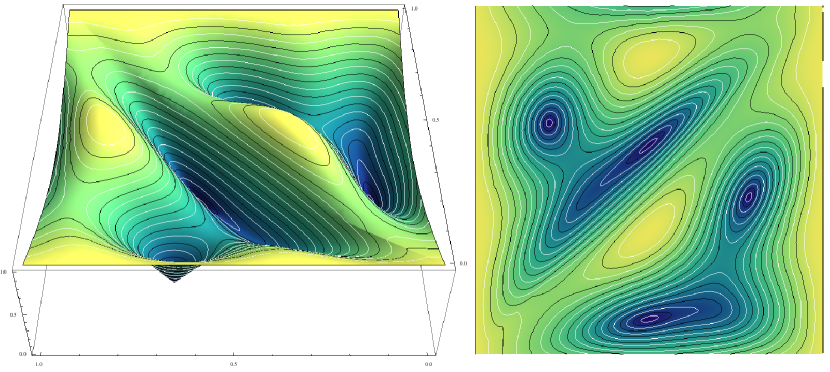
Figure 7. The graph of the norm of a piecewise-linear section of a bundle over a torus consisting of two triangles. Its two smooth parts fit continuously together along the diagonal. In this example the curvature of the bundle over each triangles is equal to $4\pi$. Note that the section has $4$ zeros - just as predicted.

In particular, using Equation (11.3), we can compute the norm of a piecewise-linear section $\tilde{\psi}$ on a given triangle $ijk$. Therefore we distinguish one of its vertices, say $i$, and write $\tilde{\psi}$ with respect to a section which is radially parallel with respect to $i$. Now, one checks that

$$|\tilde{\psi}|=|c_{i}+x_{j}(c_{j}e^{i\Omega_{ijk}x_{k}}-c_{i})+x_{k}(c_{k}e^{-i\Omega_{ijk}x_{j}}-c_{i})|,$$

where $c_{i},c_{j},c_{k}\in\mathbb{C}$ are constants depending on the explicit form of $\tilde{\psi}$. An example of the norm of a piecewise-linear section is shown in Figure 7.

As the next proposition shows, the identification of discrete and piecewise-linear sections perfectly fits together with the definitions in Section 8.

Proposition 3.

Let $\psi\in\Gamma(\mathrm{L})$ be a discrete section and let $\tilde{\psi}\in\Gamma_{pl}(\tilde{\mathrm{L}})$ be the corresponding piecewise-linear section, i.e. $\tilde{\psi}=\iota(\psi)$. Then, if $\tilde{\psi}$ has no zeros on edges, the discrete rotation form $\xi^{\psi}$ and the piecewise-smooth rotation form $\xi^{\tilde{\psi}}$ are related as follows: For each oriented edge $\ij$,

$$\xi^{\psi}_{\ij}=\int_{\ij}\xi^{\tilde{\psi}}.$$

Proof.

The claim follows easily by expressing $\tilde{\psi}$ with respect to some non-vanishing parallel section along the edge $\ij$. ∎

In particular, by Theorem 8, the index form of a non-vanishing section of a discrete hermitian line bundle with curvature counts the number of (signed) zeros of the corresponding piecewise-linear section of the associated piecewise-smooth bundle.

Let us continue with the computation of the metric on $\Gamma(\mathrm{L})$. To write down the formula we give the following definition.

Definition 17.

Let $\mathcal{X}$ be an $n$-dimensional simplicial manifold and let $\Omega\in\Omega^{2}(\mathcal{X},\mathbb{R})$. To an $n$-simplex $\sigma$ and vertices $i,j,k,l$ of $\mathcal{X}$ we assign the value

$$\Theta_{\sigma,i,j}^{\Omega}(k,l):=\frac{1}{\mathrm{vol}\,(\sigma)}\int_{\sigma}x_{k}x_{l}\,\exp\bigl{(}-\imath\sum_{m}\Omega_{\ij m}x_{m}\bigr{)},$$

where have chosen for integration an arbitrary discrete metric on $\mathcal{X}$.

Remark 12:

Note that the functions $\Theta_{\sigma,i,j}^{\Omega}$ are indeed well-defined. On a simplex, any two such measures induced by a discrete metric differ just by a constant.

With Definition 17 and Equation (11.3) we obtain the following form of the metric:

Theorem 14 (Product of Discrete Sections).

Let $\mathrm{L}$ be a discrete hermitian line bundle with curvature $\Omega$ over an $n$-dimensional Euclidean simplicial manifold $\mathcal{X}$, then the product on $\Gamma(\mathrm{L})$ induced by the associated piecewise-smooth hermitian line bundle is given as follows: Given two discrete sections $\psi=\sum_{i}\psi_{i},\phi=\sum_{i}\phi_{i}$,

$$\langle\!\langle\psi,\phi\rangle\!\rangle=\sum_{i,j}\mu_{\Omega}^{\ij}\,\langle\psi_{j},\eta_{\ij}(\phi_{i})\rangle,\quad\textit{where}\quad\mu_{\Omega}^{\ij}=\sum_{\{i,j\}\subset\sigma\in{\mathcal{X}}_{n}}\Theta_{\sigma,i,j}^{\Omega}(i,j)\,\mathrm{vol}\,(\sigma).$$

Note that $\Theta_{\sigma,i,j}^{\Omega}(k,l)$, and hence $\mu_{\Omega}^{\ij}$, can be computed explicitly using Fubini’s theorem and the following small lemma, which can be shown by induction.

Lemma 7.

Let $c\in\mathbb{C}_{\ast}$, $n\in\mathbb{N}$ and $[a,b]\subset\mathbb{R}$ be an interval. Then

$$\int_{a}^{b}x^{n}\exp(cx)dx=\Bigl{.}\frac{n!}{c^{n+1}}\Bigl{(}\sum_{k=0}^{n}(-1)^{k}\frac{(cx)^{n-k}}{(n-k)!}\Bigr{)}\exp\bigl{(}cx\bigr{)}\Bigr{|}_{a}^{b}.$$

Next, we would like to compute the Dirichlet energy of a section $\tilde{\psi}\in\Gamma_{pl}(\tilde{\mathrm{L}})$, i.e.

$$\mathrm{E}_{D}(\tilde{\psi})=\int_{\mathcal{X}}\bigl{|}\nabla\tilde{\psi}\bigr{|}^{2}.$$

Note, that the Dirichlet energy comes with a corresponding positive-semidefinite hermitian form $\langle\!\langle.,.\rangle\!\rangle_{\!D}$ - called the Dirichlet product. Clearly, like the metric, the Dirichlet product is completely determined by the values it takes on concentrated sections.

In general, if $\tilde{\psi}\neq 0$ is piecewise-linear section concentrated at $i$, it is given on the vertex star $S_{i}$ as a product $\tilde{\psi}=x_{i}\,\tilde{\phi}$, where $x_{i}$ denotes the barycentric coordinate of the vertex $i$ and $\tilde{\phi}$ is a local section radially parallel with respect to $i$. Clearly,

$$\nabla\tilde{\psi}=dx_{i}\,\tilde{\phi}+\imath\,x_{i}\,\omega_{i}\,\tilde{\phi},$$

where $\omega_{i}$ denotes the rotation form of $\tilde{\phi}$, i.e. $\nabla\tilde{\phi}=\imath\omega_{i}\,\tilde{\phi}$. Note here that $\omega_{i}$ does not depend on the actual value of $\tilde{\psi}$ at $i$, but is the same for all non-vanishing piecewise-linear sections concentrated at $i$.

To compute the rotation form $\omega_{i}$ at a given point $p_{0}\in S_{i}$, we use a local section $\zeta$ which is radially parallel with respect to $p_{0}$ such that $\zeta_{p_{0}}=\tilde{\phi}_{p_{0}}$. Then we can express $\tilde{\phi}$ in terms of $\zeta$, i.e.

$$\tilde{\phi}=z\,\zeta,$$

for some piecewise-smooth $\mathbb{C}_{\ast}$-valued function $z$ defined locally at $p_{0}$. Clearly, $|z|$ is constant, and hence

$$\left.\imath\omega_{i}\right|_{p_{0}}\,\tilde{\phi}_{p_{0}}=\left.\nabla\tilde{\phi}\right|_{p_{0}}=\left.dz\right|_{p_{0}}\,\zeta_{p_{0}}+z(p_{0})\,\left.\nabla\zeta\right|_{p_{0}}=\left.d\log z\right|_{p_{0}}\tilde{\phi}_{p_{0}}=\left.\imath d\arg z\right|_{p_{0}}\,\tilde{\phi}_{p_{0}}.$$

The clue is that we can now use the relation of parallel transport and curvature to obtain an explicit formula for $z$. If $p$ is sufficiently close to $p_{0}$, then the three points $p$, $i$ and $p_{0}$ determine an oriented triangle $\Delta^{p}$ which is contained in a simplex of $\mathcal{X}$. Its boundary curve $\gamma_{p}$ consists of three line segments $\gamma_{1},\gamma_{2},\gamma_{3}$ connecting $p$ to $i$, $i$ to $p_{0}$ and $p_{0}$ back to $p$. Hence on each of these segments either $\tilde{\phi}$ of $\zeta$ is parallel and

$$\zeta_{p}=P_{\gamma_{p}}(\tilde{\phi}_{p})=\exp\bigl{(}\imath\int_{\Delta^{p}}\tilde{\Omega}\bigr{)}\tilde{\phi}_{p}.$$

Thus we obtain that $z(p)=\exp\bigl{(}-\imath\int_{\Delta^{p}}\tilde{\Omega}\bigr{)}$ and hence

$$\Bigl{.}\omega_{i}\Bigr{|}_{p_{0}}=-\Bigl{.}d\bigl{(}\int_{\Delta^{p}}\tilde{\Omega}\bigr{)}\Bigr{|}_{p_{0}}.$$

Now, if $\Delta^{p}$ is contained in a simplex $\sigma=\{i_{0},\ldots,i_{n}\}$, one verifies that

$$\int_{\Delta^{p}}dx_{i_{j}}\wedge dx_{i_{k}}=\frac{1}{2}\bigl{(}x_{i_{j}}(p_{0})x_{i_{k}}(p)-x_{i_{k}}(p_{0})x_{i_{j}}(p)\bigr{)}.$$

Thus,

$$\Bigl{.}d\bigl{(}\int_{\Delta^{p}}\tilde{\Omega}\bigr{)}\Bigr{|}_{p_{0}} =\sum_{1\leq j<k\leq n}2\,\Omega_{i_{0}i_{j}i_{k}}\,\Bigl{.}d\bigl{(}\int_{\Delta^{p}}dx_{i_{j}}\wedge dx_{i_{k}}\bigr{)}\Bigr{|}_{p_{0}}$$

$$=\sum_{1\leq j<k\leq n}\Omega_{i_{0}i_{j}i_{k}}\,\Bigl{.}\bigl{(}x_{i_{j}}dx_{i_{k}}-x_{i_{k}}dx_{i_{j}}\bigr{)}\Bigr{|}_{p_{0}},$$

$$=\sum_{1\leq j\leq n}\Bigl{.}\bigl{(}\sum_{k\neq j}\Omega_{i_{0}i_{j}i_{k}}x_{i_{k}}\bigr{)}dx_{i_{j}}\Bigr{|}_{p_{0}}$$

and, using the convention on $\Omega$ from above, we find the following simple formula:

(11.4) $$\omega_{i}=\Bigl{.}\sum_{j}\bigl{(}\sum_{k}\Omega_{ijk}\,x_{k}\bigr{)}\,dx_{j}\Bigr{|}_{S_{i}},$$

where we sum over the whole vertex set of $\mathcal{X}$.

Now, given this local form expressions, we can finally return to the computation of the products which we are actually interested in. Therefore we consider two piecewise-linear sections concentrated at the vertices $i$ and $j$:

$$\tilde{\psi}^{i}:=\iota(\psi_{i}),\quad\tilde{\psi}^{j}:=\iota(\psi_{j}),$$

for some $\psi_{i}\in\mathrm{L}_{i}$ and $\psi_{j}\in\mathrm{L}_{j}$. On their common support $S_{i}\mathop{\cap}S_{j}$ both section can be expressed, just as above, as products of a real-valued piecewise-linear hat functions $x_{i}$ and $x_{j}$ and radially parallel local sections $\tilde{\phi}^{i}$ and $\tilde{\phi}^{j}$:

$$\tilde{\psi}^{i}=x_{i}\,\tilde{\phi}^{i},\quad\tilde{\psi}^{j}=x_{j}\,\tilde{\phi}^{j}.$$

Clearly,

$$\langle\!\langle\tilde{\psi}^{j},\tilde{\psi}^{i}\rangle\!\rangle_{\!D}= \int_{S_{i}\mathop{\cap}S_{j}}\langle dx_{j}\tilde{\phi}^{j}+\imath x_{j}\omega_{j}\,\tilde{\phi}^{j},dx_{i}\tilde{\phi}^{i}+\imath x_{i}\omega_{i}\,\tilde{\phi}^{i}\rangle$$

$$= \int_{S_{i}\mathop{\cap}S_{j}}\langle dx_{j}+\imath x_{j}\omega_{j},dx_{i}+\imath x_{i}\omega_{i}\rangle\,\langle\tilde{\phi}^{j},\tilde{\phi}^{i}\rangle.$$

With Equation (11.3) we see that

$$\langle\tilde{\phi}^{j},\tilde{\phi}^{i}\rangle=\langle\psi_{j},\eta_{\ij}(\psi_{i})\rangle\,\exp\bigl{(}-\imath\sum_{m}\Omega_{ijm}x_{m}\bigr{)}.$$

Moreover, by Equation (11.4),

$$\langle dx_{j}+\imath x_{j}\omega_{j},dx_{i}+\imath x_{i}\omega_{i}\rangle= \Bigl{[}\langle dx_{j},dx_{i}\rangle+\sum_{k^{\prime},k^{\prime\!\prime},l^{\prime},l^{\prime\!\prime}}\Omega_{ik^{\prime}l^{\prime}}\Omega_{jk^{\prime\!\prime}l^{\prime\!\prime}}x_{j}x_{i}x_{l^{\prime}}x_{l^{\prime\!\prime}}\langle dx_{k^{\prime}},dx_{k^{\prime\!\prime}}\rangle\Bigr{]}$$

$$+\imath\Bigl{[}\sum_{k^{\prime},l^{\prime}}(\Omega_{ik^{\prime}l^{\prime}}x_{i}x_{l^{\prime}}\langle dx_{j},dx_{k^{\prime}}\rangle-\Omega_{jk^{\prime}l^{\prime}}x_{j}x_{l^{\prime}}\langle dx_{k^{\prime}},dx_{i}\rangle)\Bigr{]}.$$

The constants $\langle dx_{k^{\prime}},dx_{l^{\prime}}\rangle$ are basically provided by the following lemma.

Lemma 8.

Let $\sigma=\{v_{0},\ldots,v_{n}\}$ be a Euclidean simplex of dimension $n>0$ and let $x_{i}$ denote its barycentric coordinate functions. Then

$$\mathrm{grad}\,x_{i}=-\frac{1}{h_{i}}N_{i},$$

where $h_{i}$ denotes the distance between $v_{i}$ and $\sigma_{i}=\sigma\setminus\{v_{i}\}$ and $N_{i}$ denotes the outward-pointing unit normal of $\sigma_{i}$.

Proof.

This immediately follows from two basic facts: First, $dx_{i}(v_{j}-v_{0})=\delta_{\ij}$ for $i,j>0$. Second, $h_{i}=\langle v_{0}-v_{i},N_{i}\rangle$. ∎

Lemma 8 yields almost immediately a higher dimensional analogue of the well-known cotangent formula for surfaces.

Theorem 15 (Cotangent Formula).

Let $\sigma$ be a simplex of a Euclidean simplicial complex $\mathcal{X}$ and let $\dim\sigma>1$. If $i\neq j$,

$$c_{\sigma}^{\ij}:=\int_{\sigma}\langle dx_{i},dx_{j}\rangle=\begin{cases}\hfill-\frac{1}{n(n-1)}\cot\alpha^{\ij}_{\sigma}\,\mathrm{vol}\,\bigl{(}\sigma\setminus\{i,j\}\bigr{)},\hfill&\textit{if }\{i,j\}\subset\sigma,\\ \hfill 0\hfill&else.\end{cases}$$

Here $\alpha_{\sigma}^{\ij}$ denotes the angle between the faces $\sigma\setminus\{i\}$ and $\sigma\setminus\{j\}$. Moreover,

$$c_{\sigma}^{ii}:=\int_{\sigma}|dx_{i}|^{2}=\begin{cases}\hfill\frac{1}{n\,h_{i}}\,\mathrm{vol}\,\bigl{(}\sigma\setminus\{i\}\bigr{)},\hfill&\textit{if }i\in\sigma,\\ \hfill 0\hfill&else,\end{cases}$$

where $h_{i}$ denotes the distance between the vertex $i$ and the face $\sigma\setminus\{i\}$.

Proof.

Clearly, if $\{i,j\}\not\subset\sigma$, then $\int_{\sigma}\langle dx_{i},dx_{j}\rangle=0$. Now, let $\{i,j\}\subset\sigma$, $i\neq j$. With the notation of Lemma 8, we have

$$\int_{\sigma}\langle dx_{i},dx_{j}\rangle=\langle\mathrm{grad}\,x_{i},\mathrm{grad}\,x_{j}\rangle\,\mathrm{vol}\,\sigma=\frac{\langle N_{i},N_{j}\rangle}{h_{i}h_{j}}\,\mathrm{vol}\,\sigma.$$

Furthermore, $\cos\alpha_{\sigma}^{\ij}=-\langle N_{i},N_{j}\rangle$ and $n!\,\mathrm{vol}\,\sigma=(n-2)!\,h_{i}h_{j}\sin\alpha_{\sigma}^{\ij}\,\mathrm{vol}\,\bigl{(}\sigma\setminus\{i,j\}\bigr{)}$. This yields the first part of the theorem. Similarly, $n\,\mathrm{vol}\,\sigma=h_{i}\,\mathrm{vol}\,\bigl{(}\sigma\setminus\{i\}\bigr{)}$. Setting then $i=j$ yields the second part. ∎

Definition 18.

Let $\mathcal{X}$ be an $n$-dimensional simplicial manifold and let $\Omega\in\Omega^{2}(\mathcal{X},\mathbb{R})$. Let $\sigma$ be an $n$-simplex and $i,j,k,l$ be vertices of $\mathcal{X}$. Then, let

$$\Lambda_{\sigma,i,j}^{\Omega} :=\frac{1}{\mathrm{vol}\,(\sigma)}\int_{\sigma}\exp\bigl{(}-\imath\sum_{m}\Omega_{\ij m}x_{m}\bigr{)},$$

$$\Xi_{\sigma,i,j}^{\Omega}(k,l) :=\frac{1}{\mathrm{vol}\,(\sigma)}\int_{\sigma}x_{i}x_{j}x_{k}x_{l}\,\exp\bigl{(}-\imath\sum_{m}\Omega_{\ij m}x_{m}\bigr{)},$$

where we choose for the integration an arbitrary discrete metric on $\mathcal{X}$.

Remark 13:

Just like the functions $\Theta_{\sigma,i,j}^{\Omega}$, the values $\Lambda_{\sigma,i,j}^{\Omega}$ and the functions $\Xi_{\sigma,i,j}^{\Omega}$ and are well-defined (compare Remark 12).

Now, with these definitions, we can summarize the above discussion by the following theorem.

Theorem 16 (Discrete Dirichlet Energy).

Let $\mathrm{L}$ be a discrete hermitian line bundle with curvature $\Omega$ over an $n$-dimensional Euclidean simplicial manifold $\mathcal{X}$, then the Dirichlet product on $\Gamma(\mathrm{L})$ induced by the associated piecewise-smooth hermitian line bundle is given as follows: If $\phi=\sum_{i}\phi_{i}$ and $\psi=\sum_{i}\psi_{i}$ are two discrete sections,

$$\langle\!\langle\phi,\psi\rangle\!\rangle_{\!D}=\sum_{i,j}w_{\Omega}^{\ij}\,\langle\phi_{j},\eta_{\ij}(\psi_{i})\rangle,\quad w_{\Omega}^{\ij}=\sum_{\{i,j\}\subset\sigma\in{\mathcal{X}}_{n}}W_{\sigma,i,j}^{\Omega},$$

where

(11.5) $$W_{\sigma,i,j}^{\Omega}= \Bigl{[}c^{\ij}_{\sigma}\,\Lambda_{\sigma,i,j}^{\Omega}+\sum_{k^{\prime},k^{\prime\!\prime},l^{\prime},l^{\prime\!\prime}}\Omega_{ik^{\prime}l^{\prime}}\Omega_{jk^{\prime\!\prime}l^{\prime\!\prime}}\,c_{\sigma}^{k^{\prime}k^{\prime\!\prime}}\,\Xi_{\sigma,i,j}^{\Omega}(l^{\prime},l^{\prime\!\prime})\Bigr{]}$$

$$+\imath\Bigl{[}\sum_{k^{\prime},l^{\prime}}\bigl{(}\Omega_{ik^{\prime}l^{\prime}}\,c_{\sigma}^{jk^{\prime}}\,\Theta_{\sigma,i,j}^{\Omega}(i,l^{\prime})-\Omega_{jk^{\prime}l^{\prime}}\,c_{\sigma}^{ik^{\prime}}\,\Theta_{\sigma,i,j}^{\Omega}(j,l^{\prime})\bigr{)}\Bigr{]}.$$

12. Discrete Energies on Surfaces - An Example

While the computation of the Dirichlet product $\langle\!\langle.,.\rangle\!\rangle_{\!D}$ and the metric $\langle\!\langle.,.\rangle\!\rangle$ of discrete sections is quite complicated and tedious for higher dimensional simplicial manifolds, it is manageable for the $2$-dimensional case. We are going to compute it explicitly.

Throughout this section let $\mathrm{L}$ denote a discrete hermitian line bundle with curvature $\Omega$ over a Euclidean simplicial surface $\mathcal{X}$ and let $\sigma=\{i,j,k\}$ be one of its triangles.

The metric $\langle\!\langle.,.\rangle\!\rangle$ is easily obtained. We basically just need to compute the values $\Theta_{\sigma,i,i}^{\Omega}(i,i)$ and $\Theta_{\sigma,i,j}^{\Omega}(i,j)$, which can be done over the standard triangle. We get

(12.1) $$\Theta_{\sigma,i,i}^{\Omega}(i,i)=\frac{1}{6},\quad\Theta_{\sigma,i,j}^{\Omega}(i,j)=2\frac{\exp(-\imath\Omega_{ijk})-1+\imath\Omega_{ijk}+\tfrac{1}{2}\Omega_{ijk}^{2}-\imath\tfrac{1}{6}\Omega_{ijk}^{3}}{\Omega_{ijk}^{4}}.$$

Now, we compute the Dirichlet product $\langle\!\langle.,.\rangle\!\rangle_{\!D}$ on $\mathcal{X}$. For $n=2$, the expressions $W_{\sigma,i,i}^{\Omega}$ and $W_{\sigma,i,j}^{\Omega}$ simplify drastically. First, we look at the diagonal terms. We have

$$\sum_{k^{\prime},k^{\prime\!\prime},l^{\prime},l^{\prime\!\prime}} c_{\sigma}^{k^{\prime}k^{\prime\!\prime}}\Omega_{ik^{\prime}l^{\prime}}\Omega_{ik^{\prime\!\prime}l^{\prime\!\prime}}\,\Xi_{\sigma,i,i}^{\Omega}(l^{\prime},l^{\prime\!\prime})\hfill$$

$$=\Bigl{(}c_{\sigma}^{jj}\Xi_{\sigma,i,i}^{\Omega}(k,k)-2c^{jk}_{\sigma}\Xi_{\sigma,i,i}^{\Omega}(j,k)+c_{\sigma}^{kk}\Xi_{\sigma,i,i}^{\Omega}(j,j)\Bigr{)}\Omega_{ijk}^{2},$$

and with

$$\Lambda_{\sigma,i,i}=1,\quad\Xi_{\sigma,i,i}(j,j)=\frac{1}{90}=\Xi_{\sigma,i,i}(k,k),\quad\Xi_{\sigma,i,i}(j,k)=\frac{1}{180}$$

we get the following formula:

$$W_{\sigma,i,i}^{\Omega}=c_{\sigma}^{ii}+\frac{c_{\sigma}^{jj}-c^{jk}_{\sigma}+c_{\sigma}^{kk}}{90}\Omega_{ijk}^{2}.$$

Now we would like to obtain a similar formula for the off-diagonal terms. Since $dx_{i}+dx_{j}=-dx_{k}$, we have $c_{\sigma}^{jk}+c_{\sigma}^{ki}=-c_{\sigma}^{kk}$. Hence,

$$\sum_{k^{\prime},k^{\prime\!\prime},l^{\prime},l^{\prime\!\prime}} c_{\sigma}^{k^{\prime}k^{\prime\!\prime}}\Omega_{ik^{\prime}l^{\prime}}\Omega_{jk^{\prime\!\prime}l^{\prime\!\prime}}\,\Xi_{\sigma,i,j}^{\Omega}(l^{\prime},l^{\prime\!\prime})$$

$$=-\Bigl{(}c_{\sigma}^{\ij}\Xi_{\sigma,i,j}^{\Omega}(k,k)+c_{\sigma}^{kk}\bigl{(}\Xi_{\sigma,i,j}^{\Omega}(i,j)+\Xi_{\sigma,i,j}^{\Omega}(j,k)\bigr{)}\Bigr{)}\Omega_{ijk}^{2}.$$

This time the expressions become more complicated. We get

$$\leavevmode\resizebox{465.06001pt}{}{$\Xi_{\sigma,i,j}^{\Omega}(i,j)+\Xi_{\sigma,i,j}^{\Omega}(j,k)=\frac{2}{\Omega_{ijk}^{6}}\Bigl{(}-6+4\imath\Omega_{ijk}+\Omega_{ijk}^{2}+\tfrac{1}{12}\Omega_{ijk}^{4}-\tfrac{1}{30}\imath\Omega_{ijk}^{5}+\bigl{(}6+2\imath\Omega_{ijk}\bigr{)}\exp\bigl{(}-\imath\Omega_{ijk}\bigr{)}\Bigr{)}$}.$$

Thus,

$$\sum_{k^{\prime},k^{\prime\!\prime},l^{\prime},l^{\prime\!\prime}} c_{\sigma}^{k^{\prime}k^{\prime\!\prime}}\Omega_{ik^{\prime}l^{\prime}}\Omega_{jk^{\prime\!\prime}l^{\prime\!\prime}}\,\Xi_{\sigma,i,j}^{\Omega}(l^{\prime},l^{\prime\!\prime})=$$

$$\frac{2}{\Omega_{ijk}^{4}}\Bigl{(} \bigl{[}6c_{\sigma}^{kk}-20c_{\sigma}^{\ij}\bigr{]}+\bigl{[}12c_{\sigma}^{\ij}-4c_{\sigma}^{kk}\bigr{]}\imath\Omega_{ijk}+\bigl{[}3c_{\sigma}^{\ij}-c_{\sigma}^{kk}\bigr{]}\Omega_{ijk}^{2}-\tfrac{c_{\sigma}^{\ij}}{3}\imath\Omega_{ijk}^{3}-\tfrac{c_{\sigma}^{kk}}{12}\Omega_{ijk}^{4}$$

$$+\tfrac{c_{\sigma}^{kk}}{30}\imath\Omega_{ijk}^{5}+\bigl{(}\bigr{[}20c_{\sigma}^{\ij}-6c_{\sigma}^{kk}\bigl{]}+\bigr{[}8c_{\sigma}^{\ij}-2c_{\sigma}^{kk}\bigl{]}\imath\Omega_{ijk}-c_{\sigma}^{\ij}\Omega_{ijk}^{2}\bigr{)}\exp\bigl{(}-\imath\Omega_{ijk}\bigr{)}.\Bigr{)}$$

Now, let us look at the second sum in Equation (11.5). We have

$$\imath\sum_{k^{\prime},l^{\prime}} \bigl{(}\Omega_{ik^{\prime}l^{\prime}}c_{\sigma}^{jk^{\prime}}\Theta_{\sigma,i,j}^{\Omega}(i,l^{\prime})-\Omega_{jk^{\prime}l^{\prime}}c_{\sigma}^{ik^{\prime}}\Theta_{\sigma,i,j}^{\Omega}(j,l^{\prime})\bigr{)}$$

$$=\Bigl{(}c_{\sigma}^{ii}\Theta_{\sigma,i,j}^{\Omega}(j,k)+c_{\sigma}^{jj}\Theta_{\sigma,i,j}^{\Omega}(k,i)+c_{\sigma}^{kk}\Theta_{\sigma,i,j}^{\Omega}(i,j)\Bigr{)}\imath\Omega_{ijk}.$$

The formula for $\Theta_{\sigma,i,j}^{\Omega}(i,j)$ is already given in Equation (12.1). Further, we have

$$\Theta_{\sigma,i,j}^{\Omega}(j,k)=\frac{2}{\Omega_{ijk}^{4}}\Bigl{(}3-2\imath\Omega_{ijk}-\tfrac{1}{2}\Omega_{ijk}^{2}+\bigl{(}-3+\imath\Omega_{ijk}\bigr{)}\exp\bigl{(}-\imath\Omega_{ijk}\bigr{)}\Bigr{)}=\Theta_{\sigma,i,j}^{\Omega}(k,i).$$

Thus we get

$$\imath\sum_{k^{\prime},l^{\prime}}\bigl{(}\Omega_{ik^{\prime}l^{\prime}}c_{\sigma}^{jk^{\prime}}\Theta_{\sigma,i,j}^{\Omega}(i,l^{\prime}) -\Omega_{jk^{\prime}l^{\prime}}c_{\sigma}^{ik^{\prime}}\Theta_{\sigma,i,j}^{\Omega}(j,l^{\prime})\bigr{)}=$$

$$\frac{2}{\Omega_{ijk}^{4}}\Bigl{(}\bigl{[}3(c_{\sigma}^{ii}+c_{\sigma}^{jj})-c_{\sigma}^{kk}\bigr{]} \imath\Omega_{ijk}+\bigl{[}2(c_{\sigma}^{ii}+c_{\sigma}^{jj})-c_{\sigma}^{kk}\bigr{]}\Omega_{ijk}^{2}+\tfrac{1}{2}\bigl{[}c_{\sigma}^{kk}-c_{\sigma}^{ii}-c_{\sigma}^{jj}\bigr{]}\imath\Omega_{ijk}^{3}$$

$$+\tfrac{c_{\sigma}^{kk}}{6}\Omega_{ijk}^{4}+\bigl{(} \bigl{[}c_{\sigma}^{kk}-3(c_{\sigma}^{ii}+c_{\sigma}^{jj})\bigr{]}\imath\Omega_{ijk}+\bigr{[}c_{\sigma}^{ii}+c_{\sigma}^{jj}\bigl{]}\Omega_{ijk}^{2}\bigr{)}\exp\bigl{(}-\imath\Omega_{ijk}\bigr{)}\Bigr{)}.$$

Hence, with

$$\Lambda_{\sigma,i,j}^{\Omega}=\frac{2}{\Omega_{ijk}^{4}}\Bigl{(}\Omega_{ijk}^{2}-\imath\Omega_{ijk}^{3}-\Omega_{ijk}^{2}\exp\bigl{(}-\imath\Omega_{ijk}\bigr{)}\Bigr{)},$$

Equation (11.5) becomes

$$W_{\sigma,i,j}^{\Omega}=\frac{2}{\Omega_{ijk}^{4}}\Bigl{(} \bigl{[}6\sigma^{kk}-20c_{\sigma}^{\ij}\bigr{]}+\bigl{[}12c_{\sigma}^{\ij}+3(c_{\sigma}^{ii}+c_{\sigma}^{jj})-5c_{\sigma}^{kk}\bigr{]}\imath\Omega_{ijk}+\bigl{[}4c_{\sigma}^{\ij}+2(c_{\sigma}^{ii}+c_{\sigma}^{jj}-c_{\sigma}^{kk})\bigr{]}\Omega_{ijk}^{2}$$

$$+\tfrac{1}{6} \bigl{[}3(c_{\sigma}^{kk}-c_{\sigma}^{ii}-c_{\sigma}^{jj})-8c_{\sigma}^{\ij}\bigr{]}\imath\Omega_{ijk}^{3}+\tfrac{1}{12}c_{\sigma}^{kk}\Omega_{ijk}^{4}+\tfrac{1}{30}c_{\sigma}^{kk}\Omega_{ijk}^{4}$$

$$+\bigl{(} \bigl{[}20c_{\sigma}^{\ij}-6c_{\sigma}^{kk}\bigr{]}+\bigr{[}8c_{\sigma}^{\ij}-3(c_{\sigma}^{ii}+c_{\sigma}^{jj})-c_{\sigma}^{kk}\bigl{]}\imath\Omega_{ijk}+\bigl{[}c_{\sigma}^{ii}-2c_{\sigma}^{\ij}+c_{\sigma}^{jj}]\bigr{]}\Omega_{ijk}^{2}\bigr{)}\exp\bigl{(}-\imath\Omega_{ijk}\bigr{)}\Bigr{)}.$$

Since $n=2$, the weights $c_{\sigma}^{\ij}$ are just given as follows:

$$c_{\sigma}^{\ij}=-\frac{\cot\alpha_{\sigma}^{\ij}}{2},\quad c_{\sigma}^{kk}=\frac{\ell_{\ij}}{2h_{k}},$$

where $\ell_{\ij}$ denotes the edge length. We would like to express them explicitly in terms of the Euclidean metric $g$ of $\sigma$. In fact, we can distinguish the vertex $k$ as origin and use the hat functions $x_{i}$ and $x_{j}$ as coordinates on $\sigma$. With respect to these coordinates, the metric is given by a matrix:

$$g=\begin{pmatrix}g_{11}&g_{12}\\ g_{21}&g_{22}\end{pmatrix}.$$

In terms of $g$ the cotangent weights are given as follows:

$$c_{\sigma}^{\ij} =-\frac{g_{12}}{2\sqrt{\det g}}, c_{\sigma}^{jk} =-\frac{g_{11}-g_{12}}{2\sqrt{\det g}}, c_{\sigma}^{ki} =-\frac{g_{22}-g_{12}}{2\sqrt{\det g}},$$

$$c_{\sigma}^{kk} =\frac{g_{11}-2g_{12}+g_{22}}{2\sqrt{\det g}}, c_{\sigma}^{ii} =\frac{g_{22}}{2\sqrt{\det g}}, c_{\sigma}^{jj} =\frac{g_{11}}{2\sqrt{\det g}},$$

and we have rederived the formulas in [8]:

$$W_{\sigma,i,j}^{\Omega}= \frac{1}{\mathrm{vol}\,(\sigma)\Omega_{ijk}^{4}}\Bigl{(}\bigl{[}3g_{11}+4g_{12}+3g_{22}\bigr{]}-\bigl{[}g_{11}+g_{12}+g_{22}\bigr{]}\imath\Omega_{ijk}+\tfrac{g_{12}}{6}\imath\Omega_{ijk}^{3}$$

$$+\tfrac{g_{11}-2g_{12}+g_{22}}{24}\Omega_{ijk}^{4}+\tfrac{g_{11}-2g_{12}+g_{22}}{60}\Omega_{ijk}^{4}-\bigl{(}\bigl{[}3g_{11}+4g_{12}+3g_{22}\bigr{]}$$

$$+\bigr{[}2g_{11}+3g_{12}+2g_{22}\bigl{]}\imath\Omega_{ijk}-\tfrac{1}{2}\bigl{[}g_{11}+2g_{12}+g_{22}\bigr{]}\Omega_{ijk}^{2}\bigr{)}\exp\bigl{(}-\imath\Omega_{ijk}\bigr{)}\Bigr{)}.$$

References

- [1] J. Avron, D. Osadchy, and R. Seiler. A topological look at the quantum Hall effect. Physics Today, 56:38–42, 2003.
- [2] R. Bott. On some recent interactions between mathematics and physics. Canad. Math. Bull., 28:129–164, 1985.
- [3] S. Christiansen and T. Halvorsen. A gauge invariant discretization on simplicial grids of the Schrödinger eigenvalue problem in an electromagnetic field. SIAM J. Numer. Anal., 49:331Ж345, 2011.
- [4] S. Christiansen and T. Halvorsen. A simplicial gauge theory. J. Math. Phys., 53, 2012.
- [5] M. Desbrun, E. Kanso, and Y. Tong. Discrete differential forms for computational modeling. In Discrete Differential Geometry, pages 287–324. Birkhäuser Basel, 2008.
- [6] T. Halvorsen and T. Sørensen. Simplicial gauge theory and quantum gauge theory simulation. Nuclear Physics B, 854:166–183, 2012.
- [7] A. Hatcher. Algebraic Topology. Cambridge University Press, 2002.
- [8] F. Knöppel, K. Crane, U. Pinkall, and P. Schröder. Globally optimal direction fields. ACM Trans. Graph., 32, 2013.
- [9] F. Knöppel, K. Crane, U. Pinkall, and P. Schröder. Stripe patterns on surfaces. ACM Trans. Graph., 34, 2015.
- [10] S. Kobayashi. La connexion des variétés fibrés I and II. Comptes Rendus de l’Académie Sciences, Paris, 54:318–319, 443–444, 1954.
- [11] B. Kostant. Quantization and unitary representations. In Lectures in Modern Analysis and Applications III, volume 170, pages 87–208. Springer, 1970.
- [12] C. Kreft and R. Seiler. Models of the Hofstadter type. J. Math. Phys., 37:5207–5243, 1996.
- [13] J. M. Lee. Introduction to Smooth Manifolds. Graduate Texts in Mathematics. Springer, 2012.
- [14] K. Morrison. Yang-Mills connections on surfaces and representations of the path group. Proceedings of the American Mathematical Society, 112:1101–1106, 1991.
- [15] J. R. Munkres. Elements of Algebraic Topology. Advanced book classics. Perseus Books, 1984.
- [16] M. J. Pflaum. Analytic and Geometric Study of Stratified Spaces: Contributions to Analytic and Geometric Aspects. Analytic and Geometric Study of Stratified Spaces. Springer, 2001.
- [17] K. Sasaki, Y. Kawazoe, and R. Saito. Aharonov-Bohm effect in higher genus materials. Physica A, 321:369–375, 2004.
- [18] D. J. Simms and N. M. J. Woodhouse. Lectures on Geometric Quantization. Lecture Notes in Physics. Springer Berlin Heidelberg, 1976.
- [19] A. Weil. Variétés kählériennes. Actualités Scientifiques et Industrielles. Hermann, 1958.
- [20] S. Weißmann, U. Pinkall, and P. Schröder. Smoke rings from smoke. ACM Trans. Graph., 33, 2014.