June 2015

ABSTRACT

In this work nonperturbative aspects of quantum gravity are investigated using the lattice formulation, and some new results are presented for critical exponents, amplitudes and invariant correlation functions. Values for the universal scaling dimensions are compared with other nonperturbative approaches to gravity in four dimensions, and specifically to the conjectured value for the universal critical exponent $\nu=1/3$. It is found that the lattice results are generally consistent with gravitational anti-screening, which would imply a slow increase in the strength of the gravitational coupling with distance, and here detailed estimates for exponents and amplitudes characterizing this slow rise are presented. Furthermore, it is shown that in the lattice approach (as for gauge theories) the quantum theory is highly constrained, and eventually by virtue of scaling depends on a rather small set of physical parameters. Arguments are given in support of the statement that the fundamental reference scale for the growth of the gravitational coupling $G$ with distance is represented by the observed scaled cosmological constant $\lambda$, which in gravity acts as an effective nonperturbative infrared cutoff. In this nonperturbative vacuum condensate picture a fundamental relationship emerges between the scale characterizing the running of $G$ at large distances, the macroscopic scale for the curvature as described by the observed cosmological constant, and the behavior of invariant gravitational correlation functions at large distances. Overall, the lattice results suggest that the slow infrared growth of $G$ with distance should become observable only on very large distance scales, comparable to $\lambda$. It is hoped that future high precision satellite experiments will possibly come within reach of this small quantum correction, as suggested by a vacuum condensate picture of quantum gravity.

1 Introduction

In this work nonperturbative aspects of the ground state for quantum gravity will be discussed, based on the lattice theory. So far the lattice formulation represents the only known first-principle method for reproducing correctly the low energy properties of non-Abelian gauge theories, including confinement and chiral symmetry breaking. It is hoped therefore that a lattice approach to quantum gravity will shed useful light on the low energy properties of quantum gravity as well. A key aspect of this method is a recognition of the importance of Wilson’s modern interpretation of the renormalization group [1, 2] as it applies to perturbatively non-renormalizable theories [3, 4], including gravity. In previous work the elegant lattice formulation of gravity of Regge and Wheeler [5, 6] was used to compute a number of observable quantities expected to be relevant for the ground state properties of quantum gravity (for a detailed discussion of the Feynman path integral approach to quantum gravity the reader is referred to [7]). The lattice formulation implies the existence of an ultraviolet cutoff, nevertheless in the real world such a cutoff would presumably arise from short distance details derived from an underlying more fundamental theory, such as higher derivative gravity, supergravity or string theory. Nevertheless, it is expected that a softer cutoff would lead to significant short distance modifications of gravity, while leaving the quantum infrared behavior largely unchanged. It is these universal long distance effects that form the subject of the present paper. As in QED and QCD, it will turn out that these quantum infrared modifications to gravity are intrinsically non-local.

In four dimensions (and for the Euclidean theory) it was found that for gravity two phases are possible, a pathological gravitational screening phase for $G<G_{c}$, and an anti-screening phase for $G>G_{c}$. It has been known for some time that the screening phase corresponds to a branched polymer, with no physically acceptable continuum limit, and the lattice results were therefore interpreted as suggesting that ultimately the only physical acceptable phase is the strong coupling phase for $G>G_{c}$. Furthermore, it was found that in this phase the average local curvature approaches zero towards the critical point at $G_{c}$, indicating that in this phase the recovery of the semiclassical limit for gravity appears to be possible. In previous work detailed estimates were given for the location of the critical point at $G_{c}$, for the critical exponents and scaling dimensions characterizing the growth of the gravitational coupling with distance, and for the scaling behavior of gravitational correlation functions. Of central importance in these results is the value for the universal critical exponent $\nu$, related to the derivative of the beta function for $G$ at the fixed point. Here more refined estimates for the critical point and scaling dimensions will be provided; the analysis will later be extended to correlation functions of invariant operators at fixed geodesic distances. In this context the present discussion includes both local operators, as well as extended ones such as the Wilson loop and the correlation between gravitational Wilson loops. In previous work it was argued that the gravitational Wilson loop provides information about the macroscopic curvature, and therefore about the hoped-for recovery of the semiclassical limit. This last result is quite different from what is found in gauge theories, since in gravity the gravitational Wilson loop has no significance for the static potential. Also, it was shown earlier that the the area law for the gravitational Wilson loop provides a connection between the nonperturbative scale $\xi$ that arises in nonperturbative gravity and the macroscopic large-scale curvature, and thus the observed effective cosmological constant $\lambda$. Here it will be argued that the numerical results so far are consistent with many of the previous answers, including the conjecture that the exponent $\nu$ is exactly equal to one third in four dimensions. The latter part of the paper will therefore deal with a detailed discussion of the possible physical significance of having an exponent $\nu$ exactly equal to one third in four dimensions, as this relates to a number of physical consequences, such as the scale dependence of $G$ and the behavior of invariant gravitational correlation functions at large separation.

The structure of the paper is as follows. In Section 2 the form of the discretized lattice gravitational Feynman path integral will be recalled, and basic notation will be established. Here the basic definitions for local averages and their fluctuations will be laid out as well. Section 3 will introduce basic diffeomorphism invariant correlation functions, and show how these can be transcribed to the lattice theory. Section 4 will extend the previous discussion to correlation functions involving operators that are not necessarily local, such as the correlation between smeared operators, the definition of the gravitational Wilson loop, and the form and basic expected properties of correlations between these loop operators. Section 5 will recall the basic fundamental scaling assumptions for the gravitational path integral, and how those assumptions and definitions affect the critical behavior of various averages, fluctuations and correlations defined in the previous sections. Section 6 summarize how the quantum continuum limit in lattice quantum gravity should be taken, in accordance with the general principles of the renormalization group. A discussion is provided to show how the interplay between the bare coupling constants, the critical point and the correlation length $\xi$ lead to a definite expression for the running of Newton’s $G$. In addition, it is shown how the prediction for a running of $G$ can be described in terms of universal quantities, to leading order in the vicinity of that fixed point, and specifically in terms of universal exponents and amplitudes. Sections 7,8,9 and 10 later provide details on the how the numerical calculations are performed, and on the methods by which the universal critical exponents and amplitudes are extracted from the numerical results. A discussion is given to show the overall consistency of the results, based on a variety of different observables and methods of analysis. At the end of Section 10 the results obtained from a variety of different observables are compared in a comprehensive summary table. Two additional tables later provide a comparison between the lattice results for the universal exponents and the values obtained by other nonperturbative methods. In Section 10 a separate comparison table is provided for four dimensions, and a second table is added later for the case of three dimensions. It is argued that the numerical results so far are consistent with the expectation that the universal critical exponent $\nu$ for quantum gravity in four dimensions is equal to one third. Section 11 then discusses the physical implications of having an exponent $\nu$ exactly equal to one third as it applies to various local averages, fluctuations and correlation functions introduced earlier in the paper. It is shown that many lattice results become particularly simple and perhaps more transparent for this choice of exponent. The numerical calculation also supply a value for several critical amplitudes which appear in the running of $G$ in the vicinity of the fixed point at $G_{c}$. Section 12 at the end of the paper is devoted to a discussion of the curvature correlation function, and how this correlation can, in suitable cases via the field equations, be related to the analogous correlation function for matter density fluctuations. The final section presents some conclusions, and elaborates further on a suggestive analogy between the vacuum condensate picture derived from lattice quantum gravity and the well understood nonperturbative properties of non-Abelian gauge theories, and specifically the case of lattice $QCD$.

2 Path Integral, Invariant Local Gravitational Averages and their Fluctuations

In this section the basic definitions for diffeomorphism invariant gravitational averages and correlations will be recalled briefly, in a form suitable for later discussions. Here the starting point for a nonperturbative formulation of quantum gravity is the discretized form for the Feynman path integral for pure gravity [8], written originally as

$$Z_{C}\;=\;\int d\mu[g_{\mu\nu}]\;\exp\left\{-I[g_{\mu\nu}]\right\}\;\;,$$ (1)

with invariant gravitational action

$$I[g_{\mu\nu}]\;=\;\int d^{4}x\,\sqrt{g}\,\Bigl{(}\lambda_{0}-{k\over 2}\,R+{a_{0}\over 4}\,R_{\mu\nu\rho\sigma}R^{\mu\nu\rho\sigma}+\cdots\Bigr{)}$$ (2)

and DeWitt invariant functional measure [9]

$$\int d\mu[g_{\mu\nu}]\;=\;\int\prod_{x}\;\left({\textstyle\sqrt{g(x)}\displaystyle}\right)^{\sigma}\;\prod_{\mu\geq\nu}\,dg_{\mu\nu}(x)\;.$$ (3)

In the above expression $k^{-1}\equiv 8\pi G$ with $G$ the bare Newton’s constant, $\lambda_{0}$ the bare cosmological constant, and $a_{0}$ a possible higher derivative coupling [10]. In the absence of matter fields the DeWitt invariant measure for pure gravity in four dimensions corresponds to the simple choice $\sigma=0$. In the following we will only consider the case $a_{0}=0$, i.e. no higher derivative $R^{2}$-type terms.

The continuum Feynman path integral given above is generally ill-defined, and has to be formulated more precisely by introducing a suitable discretization [13]. The last step is particularly important for nonperturbative calculations, where the nontrivial invariant measure over the $g_{\mu\nu}$’s plays a key role. Regge and Wheeler proposed an elegant discretization of the classical gravitational action [5, 6], which forms the basis for the lattice formulation of quantum gravity discussed in this paper. Once the measure and the path integral have been discretized, the ultimate goal then becomes to recover the original continuum theory of Eq. (1) in the limit of a small lattice spacing (this limit is rather subtle, and involves in a nontrivial way fundamental aspects of the renormalization group). This approach then leads, as a starting point, to the following discrete form for the Euclidean Feynman path integral for pure gravity

$$Z_{L}\;=\;\int d\mu[l^{2}]\exp\left\{-I[l^{2}]\right\}\;\;,$$ (5)

with lattice gravitational action

$$I[l^{2}]\;=\;\sum_{h}\,\Bigl{(}\lambda_{0}\,V_{h}-k\,\delta_{h}A_{h}+a\,\delta_{h}^{2}A_{h}^{2}/V_{h}+\cdots\Bigr{)}$$ (6)

and lattice functional measure

$$\int d\mu[l^{2}]\;=\;\int_{0}^{\infty}\;\prod_{s}\;\left(V_{d}(s)\right)^{\sigma}\;\prod_{ij}\,dl_{ij}^{2}\;\Theta[l_{ij}^{2}]\;.$$ (7)

Here the sum over hinges $h$ in four dimensions corresponds to a sum over all lattice triangles with area $A_{h}$, with deficit angles $\delta_{h}$ describing the curvature around them.

In the discrete formulation a functional integration over metric is replaced by an integration over squared edge lengths, which are taken as fundamental variables in the discrete theory. The basis for this step is a rather direct correspondence between the squared edge lengths in a four-simplex and the induced metric within that same simplex. Within each $n$-simplex $s$ one can define a metric in terms of unit vectors $e_{i}$ pointing along the edges

$$g_{ij}(s)\;=\;e_{i}\cdot e_{j}\;\;,$$ (8)

with $1\leq i,j\leq n$, and a positive definite quantity in the Euclidean case. In terms of the edge lengths $l_{ij}\,=\,|e_{i}-e_{j}|$, or conversely

$$g_{ij}(s)\;=\;\textstyle{1\over 2}\displaystyle\,\left(l_{0i}^{2}+l_{0j}^{2}-l_{ij}^{2}\right)\;\;$$ (9)

for a simplex based at $0$. This last result then provides a key connection between the metric $g_{\mu\nu}(x)$ in the continuum and the lattice degrees of freedom $l^{2}_{i}$, which is essential in establishing a fairly unambiguous relationship between lattice and continuum operators, just as is the case in ordinary lattice gauge theories. It is also known that the lattice action in Eq. (5 generally reduces to the continuum one of Eq. (1 for smooth enough field configurations [17], and that it contains the correct physical degrees of freedom for gravity in the weak field limit, namely transverse-traceless (massless spin two) modes [18].

The general aim of the calculations presented later will be to evaluate the lattice path integral exactly by numerical means, by performing a (correctly weighted) sum over all fields configurations, without relying on the weak field expansion, or an expansion around suitable saddle points or some other approximate scheme, which generally tends to involve a number of assumptions on what configurations (smooth or otherwise) might or might not play a dominant role in the path integral (indeed the general expectation for such path integrals is that smooth field configurations tend to have measure zero). Here the functional integration over edge lengths is highly nontrivial, due to the constraint coming from the generalized triangle inequalities [expressed in the function $\Theta[l_{ij}^{2}]$ in Eq. (7)], which is placed there in the Euclidean formulation to insure that all edge lengths, triangle areas, tetrahedra and simplex volumes are strictly positive. The discrete gravitational measure in $Z_{L}$ of Eq. (5) can then be regarded as a regularized version of the DeWitt continuum functional measure [9]. Also, a bare cosmological constant term is essential for the convergence of the path integral, while curvature squared terms allow one to further control the fluctuations in the curvature [14, 19]. It is generally understood that these last terms are generated by radiative corrections within a perturbative diagrammatic treatment in the continuum. In practice, and for obvious phenomenological reasons, one is nevertheless only interested eventually in a limit where effective higher derivative contributions are negligible compared to the rest of the action, $a_{0}\rightarrow 0$.

In this limit the theory depends, in the absence of matter and after a suitable rescaling of the metric (in the continuum) or the edge lengths (on the lattice), only on one bare parameter, the dimensionless coupling $k/\sqrt{\lambda_{0}}$. Indeed already in the continuum one finds in $d$ dimensions under a rescaling of the metric

$$g_{\mu\nu}=\omega\,g_{\mu\nu}^{\prime}\;,$$ (10)

with $\omega$ a constant, that the cosmological constant term $\lambda_{0}\sqrt{g}$ turns into $\lambda_{0}\,\omega^{d/2}\,\sqrt{g^{\prime}}$ so that a subsequent rescaling

$$G\rightarrow\omega^{-d/2+1}G\;,\;\;\;\;\lambda_{0}\rightarrow\lambda_{0}\,\omega^{d/2}$$ (11)

leaves only the dimensionless combination $G^{d}\lambda_{0}^{d-2}$ unchanged. Clearly only the latter combination has physical meaning in pure gravity, and in particular one can always choose the scale $\omega=\lambda_{0}^{-2/d}$ so as to adjust the volume term to have a unit coefficient. Equivalently, this shows that it seems physically meaningless to discuss separately the renormalization properties of $G$ and $\lambda_{0}$. Without any loss of generality one can therefore set the bare cosmological constant $\lambda_{0}=1$ in units of the ultraviolet cutoff [14]. The latter contribution controls the overall scale for the edge lengths, contains (like a mass term) no derivatives in the continuum, and does not affect the construction of a suitable lattice continuum limit, which is determined by the relative interplay between the curvature and volume terms. It seems therefore redundant to vary $\lambda_{0}$, as this will only change the overall length scale, without any discernible effect on the quantum lattice continuum limit. In the continuum a similar result can be derived; there on can show that the renormalization of $\lambda_{0}$ is gauge- and scheme-dependent, and that only the renormalization of $G$ is independent of the choice of gauge condition [22, 23, 24].

Some partial information about the behavior of physical correlations can be obtained indirectly from averages of suitable local invariant operators. In [19] a set of diffeomorphism invariant gravitational observables, such as the average curvature and its fluctuation, were introduced. Appropriate lattice analogs of these quantities are easily written down, making use of the following well understood correspondences

$$\sqrt{g}\,(x)\; \to \;\sum_{{\rm hinges}\,h\,\supset\,x}\;V_{h}$$

$$\sqrt{g}\,R(x)\; \to \;2\sum_{{\rm hinges}\,h\,\supset\,x}\;\delta_{h}A_{h}$$

$$\sqrt{g}\,R_{\mu\nu\lambda\sigma}\,R^{\mu\nu\lambda\sigma}(x)\; \to \;4\sum_{{\rm hinges}\,h\,\supset\,x}\;(\delta_{h}A_{h})^{2}/V_{h}\;\;.$$ (12)

An overall numerical normalization coefficient has been omitted on the r.h.s., since it will depend on how many hinges are actually included in the summation. In the following we will not consider any further higher derivative terms, which means that the subsequent discussion will be limited almost exclusively to the first and second type of operators.

First consider the average local curvature, defined as

$${\cal R}(k)\;\sim\;{<\int d^{4}x\,\sqrt{g}\,R(x)>\over<\int d^{4}x\,\sqrt{g}>}\;\;\;.$$ (13)

The above quantity is relevant for parallel transports of vectors around an elementary, infinitesimal parallel transport loop, and is by construction manifestly diffeomorphism invariant. On the lattice one first notes that it is preferable to define quantities in such a way that variations in the average lattice spacing $l_{0}\sim\sqrt{<\!l^{2}\!>}$ are compensated by a suitable multiplicative factor, determined entirely from dimensional considerations. It would be possible to adjust $\lambda_{0}$ in Eq. (5) to achieve $l_{0}=1$, but here we choose to have simply $\lambda_{0}=1$ in units of the ultraviolet cutoff $\Lambda=1/a$. As stated previously, in the following all quantities will be expressed in units of this fundamental cutoff $a$, whose value, as is customary in lattice gauge theories, is set initially equal to one, $a=1$. In the case of the average local curvature a useful lattice definition is therefore [19, 14]

$${\cal R}(k)\;\equiv\;<\!l^{2}\!>{<2\;\sum_{h}\delta_{h}A_{h}>\over<\sum_{h}V_{h}>}\;\;\;.$$ (14)

Note that by construction this quantity is dimensionless, and consequently if all edge lengths are rescaled by a common factor it remains unchanged. Again, this choice factors out an entirely irrelevant overall length scale (a phenomenon peculiar to gravity, which does not arise in ordinary lattice gauge theories).

A second quantity of interest is the local curvature fluctuation

$$\chi_{\cal R}(k)\;\sim\;{<(\int d^{4}x\,\sqrt{g}\,R)^{2}>-<\int d^{4}x\,\sqrt{g}\,R>^{2}\over<\int d^{4}x\,\sqrt{g}>}\;\;.$$ (15)

A suitable lattice transcription of this last quantity is

$$\chi_{\cal R}(k)\;\equiv\;{<(\sum_{h}2\,\delta_{h}A_{h})^{2}>-<\sum_{h}2\,\delta_{h}A_{h}>^{2}\over<\sum_{h}V_{h}>}\;\;\;.$$ (16)

Note that in the functional integral formulation of Eqs. (1) and (5) both the average curvature ${\cal R}(k)$ and its fluctuation $\chi_{\cal R}(k)$ can be obtained by taking derivatives of the functional $Z_{L}$ in Eq. (5) with respect to $k$. Therefore on the lattice one has

$${\cal R}(k)\,\sim\,\frac{1}{<\!V\!>}\,\frac{\partial}{\partial k}\ln Z_{L}\;$$ (17)

and

$$\chi_{\cal R}(k)\,\sim\,\frac{1}{<\!V\!>}\,\frac{\partial^{2}}{\partial k^{2}}\ln Z_{L}\;,$$ (18)

just as the analogous continuum quantities in Eqs. (13) and (15) can be obtained as derivatives of the expression in Eq. (1). In a similar way, the average volume per site is defined as

$$<\!V\!>\;\equiv\;{1\over N_{0}}<\sum_{h}V_{h}>\;\;\;,$$ (19)

and again one has

$$<\!V\!>\;=\;-\,\frac{\partial}{\partial\lambda_{0}}\,{1\over N_{0}}\,\ln Z_{L}\;\;\;.$$ (20)

Furthermore, its fluctuation $\chi_{V}$ can also be obtained as a second derivative of $Z_{L}$ with respect to the bare cosmological constant $\lambda_{0}$. A simple scaling argument, based on neglecting the effects of curvature terms entirely (which vanish in the vicinity of the critical point), is found to give a rather accurate estimate for the average volume per edge

$$<\!V_{l}\!>\;\sim\;{2\,(1+\sigma d)\over\lambda_{0}\,d}\;\;\mathrel{\mathop{\rightarrow}_{d=4,\;\sigma=0}}\;\;{1\over 2\,\lambda_{0}}\;\;.$$ (21)

In four dimensions numerical simulations agree quite well with this simple formula. Finally, a set of exact sume rules can be derived from the scaling properties of the action and measure in Eq. (5). As an example, for the case of the $dl^{2}$ measure one finds the following exact lattice Ward identity

$$2\lambda_{0}<\sum_{h}V_{h}>\;-\;k<\sum_{h}\delta_{h}A_{h}>\;-\;N_{1}\;=\;0\;\;\;,$$ (22)

which is easily derived from Eq. (5) and the definitions in Eqs. (17) and (20). Here $N_{0}$ represents the number of sites in the lattice, and the averages are defined per site. For the hypercubic lattices used in this paper, $N_{1}=15\,N_{0}$, $N_{2}=50\,N_{0}$, $N_{3}=36\,N_{0}$ and $N_{4}=24\,N_{0}$. The above exact identity can be a useful tool in establishing the numerical convergence of the integration method used for the lattice path integral.

3 Diffeomorphism Invariant Gravitational Correlation Functions

Generally in a quantum theory of gravity the physical distance between any two points $x$ and $y$ in a fixed background geometry is determined by the metric

$$d(x,y\,|\,g)\;=\;\min_{\xi}\;\int_{\tau(x)}^{\tau(y)}d\tau\sqrt{\textstyle g_{\mu\nu}(\xi){d\xi^{\mu}\over d\tau}{d\xi^{\nu}\over d\tau}\displaystyle}\;\;.$$ (23)

Because of quantum fluctuations the latter depends on the metric or, equivalently, in the lattice case on the edge length configuration considered. Correlation functions of local operators need to account for this fluctuating distance, and as a result these correlations have to be computed at some fixed geodesic distance between a set of given spacetime points [14, 25]. In addition, in gravity one generally requires that the local operators involved should be coordinate scalars. In principle one could also smear such operators over a small region of spacetime, an option which will be discussed later. It is also possible to compute nonlocal gravitational observables in analogy to what is done in Yang-Mills theories, by defining objects such as the gravitational Wilson loop (which carries information about the parallel transport of vectors around large loops, and therefore about large scale curvature) [26, 27, 28, 29], or the correlation between Wilson lines closed by the lattice periodicity (which can be used for extracting the static potential in quantum gravity) [30, 31]. One more different type of gravitational correlation was studied in [32].

A fundamental correlation function in te quantum theory of gravity is the one associated with the scalar curvature, with physical points $x$ and $y$ separated by a fixed geodesic distance $d$

$$G_{R}(d)\;\sim\;<\sqrt{g}\;R(x)\;\sqrt{g}\;R(y)\;\delta(|x-y|-d)>_{c}\;.$$ (24)

It is then straightforward to define the same type of object on the lattice. If the lattice deficit angles are averaged over a number of contiguous hinges which share a common vertex, one is lead to consider the connected lattice correlation function at fixed geodesic distance $d$

$$G_{R}(d)\;\equiv\;<\sum_{h\supset x}2\,\delta_{h}A_{h}\;\sum_{h^{\prime}\supset y}2\,\delta_{h^{\prime}}A_{h^{\prime}}\;\delta(|x-y|-d)>_{c}\;.$$ (25)

The need to compute physical distances between points for any given metric (or edge length) field configuration complicates the problem considerably, as compared for example to ordinary gauge theories, where the distance between points is assigned a priori based on a fixed immutable underlying lattice structure.

For the curvature correlation at fixed geodesic distance one expects at short distances (i.e. distances much shorter than the gravitational correlation length $\xi$) a power law decay

$$<\sqrt{g}\;R(x)\;\sqrt{g}\;R(y)\;\delta(|x-y|-d)>_{c}\;\;\mathrel{\mathop{\sim}_{d\;\ll\;\xi}}\;\;d^{-2n}\;\;\;\;,$$ (26)

with the power characterized by a universal exponent $n$; how $n$ is related to another calculable universal critical exponent (in particular $\nu$) will be discussed further below.

One notes on the other hand that for sufficiently strong coupling (large $G$, or small $k$) fluctuations in different spacetime regions largely decouple (the kinetic or derivative term in Eqs. (1) or (5) is responsible for coupling fluctuations in different regions, and it comes with a coefficient $1/G$). In this regime one then expects a faster, exponential decay, controlled by the correlation length $\xi$

$$<\sqrt{g}\;R(x)\;\sqrt{g}\;R(y)\;\delta(|x-y|-d)>_{c}\;\;\mathrel{\mathop{\sim}_{d\;\gg\;\xi}}\;\;e^{-d/\xi}\;\;\;\;.$$ (27)

This last result shows that the fundamental gravitational correlation length $\xi$, if nonzero, can be defined through the long-distance decay of the connected invariant correlations at fixed geodesic distance $d$. Note also that the behavior in Eq. (26) is expected to hold at short distances, i.e. distances much larger than the fundamental lattice spacing but significantly shorter than the correlation length, $l_{0}\ll d\ll\xi$, whereas the behavior in Eq. (27) is expected to hold at much larger distances, $d\gg\xi\gg l_{0}$. In either case, in order to reach the lattice continuum limit the distances considered need to be much larger than the fundamental lattice spacing, $d,\xi\gg l_{0}$. This last constraint is referred to as the scaling limit, where short distance lattice artifacts are presumably washed out, and the true (and physically relevant) continuum limit is expected to emerge. Later it will be shown, from rather elementary scaling considerations, that the exponent $n$ in Eq. (26) is related to the so-called correlation length exponent $\nu$ in four dimensions by $n=4-1/\nu$.

Another key result of relevance here lies in the fact that the local curvature fluctuation defined in Eqs. (15) and (16) is directly related to the connected curvature correlation of Eqs. (24) and (25) at zero momentum

$$\chi_{\cal R}\;\sim\;{\int d^{4}x\int d^{4}y<\sqrt{g(x)}\,R(x)\;\sqrt{g(y)}\,R(y)>_{c}\over<\int d^{4}x\sqrt{g(x)}>}\;\;\;,$$ (28)

a well-known and rather useful result already in ordinary field theories. This connection will be used extensively further below, and its relevance will lie in the fact that it allows one to relate the exponent $\nu$, obtained for example from the curvature fluctuation of Eq. (15), to the physical correlation in Eqs. (24) and (26). The latter can in turn be related to other physical correlations, such as the matter density correlation, by the use for example of the effective, long distance gravitational field equations.

4 Correlations Between Smeared and Nonlocal Operators

The discussion up to this point has dealt with local operators and their correlations, i.e. operators defined at a point $x$ in spacetime, or on the lattice at a single lattice point. Some rather mild nonlocality does in fact appear, due to the circumstance that the gravitational action involves, via the affine connection and the Riemann tensor, the parallel transport of a test vector around an infinitesimally small loop. The latter is encoded on the lattice by the deficit angles, which describe the parallel transport of a vector around a loop whose size is comparable to the lattice spacing, or in physical terms of size comparable to the ultraviolet cutoff or the Planck length. It is nevertheless possible to define smeared operators, which involve a new length scale: the linear size of the smearing volume $r_{s}$. On the basis of rather general renormalization group arguments one expects correlations for these operators to have milder short distance divergences.

Consider first the average of an operators over a spherically shaped smearing region $\Omega(x,r_{s})$, centered at the point $x$ and of linear size $r_{s}$. In other words, all points within a physical distance $r_{s}$ from the point in question are considered; on a lattice of course the number of points within a given physical neighborhood of the point $x$ with linear size $r_{s}$ will in general be finite. Then define the smeared operator ${\cal O}_{S}(x)$ by the spacetime average

$${\cal O}_{S}(x)\;\equiv\;\int_{\Omega(x,r_{s})}d^{4}z\,\sqrt{g}\;{\cal O}(z)\;\;.$$ (29)

A natural candidate operator for smearing is of course the scalar curvature, but various curvature squared terms would also be viable, for example. A suitable invariant correlation function is then defined as

$$G_{r_{s}}(d)\;=\;<{\cal O}_{S}(x)\;{\cal O}_{S}(y)\;\delta(|x-y|-d)>_{c}\;,$$ (30)

where again the correlation between the two operators ${\cal O}_{S}(x)$ is taken at a fixed geodesic distance $d$. The general expectation is that the short distance ($d\mathrel{\hbox to0.0pt{\lower 4.0pt\hbox{\hskip 1.0pt$\sim$}\hss}\raise 1.0pt\hbox{$>$}}r_{s}$) behavior for this correlation function is less singular than for correlations of operators defined at a single point. Nevertheless at larger distances $d\gg r_{s}$ the asymptotic decay of the correlation function should be the same as for the one in Eq. (26), provided the operators in question have the same quantum numbers.

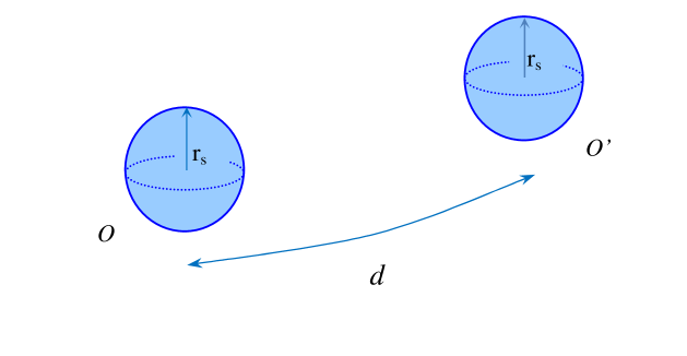
Figure 1: Correlation function for two smeared operators of size $r_{s}$, separated by a geodesic distance $d$.

A second class of invariant correlation functions for smeared operators involves the correlation of parallel transport loops [28, 26]. First note that infinitesimal transport loops appear already in the definition of the correlation function for the local scalar curvature, as in Eqs. (24) and (25). Next consider the parallel transport of a vector around a loop $C$ which is not infinitesimal; in the following this loop will be assumed to be close to planar, a well defined geometric construction described in detail in [29]. First define the total rotation matrix ${\bf U}(C)$ along the path $C$ via a path-ordered (${\cal P}$) exponential of the integral of the affine connection $\Gamma^{\lambda}_{\mu\nu}$

$$U^{\mu}_{\;\;\nu}(C)\;=\;\Bigl{[}\;{\cal P}\,\exp\left\{\oint_{C}\Gamma^{\cdot}_{\lambda\,\cdot}dx^{\lambda}\right\}\,\Bigr{]}^{\mu}_{\;\;\nu}\;\;.$$ (31)

The lattice action itself already contains contributions from infinitesimal loops, but more generally one might want to consider near-planar, but noninfinitesimal, lattice closed loops $C$. Along such a closed loop the overall rotation matrix is given by a product of elementary rotations defined along the lattice path

$$U^{\mu}_{\;\;\nu}(C)\;=\;\Bigl{[}\prod_{s\,\subset C}U_{s,s+1}\Bigr{]}^{\mu}_{\;\;\nu}\;.$$ (32)

In analogy with the infinitesimal loop case, one expects for the overall rotation matrix

$$U^{\mu}_{\;\;\nu}(C)\;\approx\;\Bigl{[}\,e^{\delta(C)\omega(C))}\Bigr{]}^{\mu}_{\;\;\nu}\;\;,$$ (33)

where $\omega_{\mu\nu}(C)$ is an area bivector perpendicular to the loop and $\delta(C)$ the corresponding deficit angle. This will work if the loop is close to planar, so that $\omega_{\mu\nu}$ can be taken to be approximately constant along the path $C$, or defined by some suitable average over the loop. Here by a near-planar loop around the point $P$ what is meant is a loop that is constructed by drawing outgoing geodesics on a plane through $P$, so that this unit bivector plays the role of a normal to the loop. A coordinate scalar can be defined by contracting the above rotation matrix ${\bf U}(C)$ with the appropriate unit length bivector, namely

$$W_{C}\;=\;\omega_{\mu\nu}(C)\;U^{\mu\nu}(C)$$ (34)

where the bivector $\omega_{\alpha\beta}(C)$ is taken to be representative of the overall geometric features of the loop. Now if the parallel transport loop in question is centered at the point $x$, then one can define the operator $W_{C}(x)$ by

$$W_{C}(x)\;=\;\omega_{\mu\nu}(C,x)\;U^{\mu\nu}(C,x)$$ (35)

with the near-planar loop centered at $x$ and of linear size $r_{C}$. A suitable invariant correlation two-point function for these operators is then defined as

$$G_{C}(d)\;=\;<W_{C}(x)\;W_{C}(y)\;\delta(|x-y|-d)>_{c}\;\;,$$ (36)

where again the correlation between the loop operators $W_{C}(x)$ is taken at some given fixed geodesic distance $d$. Of course for infinitesimal loops one recovers the expressions given earlier in Eqs. (24) and (25).

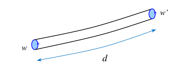
Figure 2: Correlation function of two infinitesimal parallel transport loops, separated by a geodesic distance $d$.

In general one needs to specify the relative orientation of the two loops. So, for example, one can take the first loop in a plane perpendicular to the direction associated with the geodesic connecting the two points, and the same for the second loop; the parallel transport of a vector along this geodesic will then be sufficient to establish the relative orientation of the two loops. Nevertheless if one is interested in the analog (for large loops) of the scalar curvature, then it will be adequate to perform a weighted sum over all possible loop orientations at both ends. This is in fact precisely what is done for infinitesimal loops of size $r_{C}\sim a$, if one looks carefully at the way the Regge lattice action is originally defined. Again here the expectation is that the short distance $d\mathrel{\hbox to0.0pt{\lower 4.0pt\hbox{\hskip 1.0pt$\sim$}\hss}\raise 1.0pt\hbox{$>$}}r_{C}$ behavior of this correlation function for extended loop objects is less singular than for correlations of operators defined at a point; nevertheless at larger distances $d$ such that $r_{C}\ll d\ll\xi$ the decay of these correlation function should be the same as the local ones in Eq. (26).

It is possible to give a more quantitative description for the behavior of the loop-loop correlation function given in Eq. (36), at least in the strong coupling limit. The following estimate is based on the previous results and definitions, and the important analogy and correspondence of lattice gravity to non-Abelian gauge theories outlined in [33, 29]. First it will be assumed here that the two (near planar) loops are of comparable shape and size, with overall linear sizes $r_{C}\sim L$ and perimeter $P\simeq 2\pi L$. In addition, the two loops will be separated by a distance $d\gg L$, and for both loops it will be assumed that this separation is much larger than the lattice spacing, $d\gg a$ and $L\gg a$. Then to get a nonvanishing correlation in the strong coupling, large $G$ limit it will be necessary to completely tile a tube connecting the two loops, due to the area law arising from the use of the Haar measure for the local rotation matrices at strong coupling, again as discussed in detail in [29]. In this last paper extensive use is made of a modified first order formalism for the Regge lattice theory, based on the work of [34], which then allows the separation of metric degrees of freedom into local Lorentz rotations and tetrads, as is done in the continuum. Consequently in this limit one obtains an area law

$$G_{C}(d)\;\simeq\;\exp\left\{-\,{2\pi L\cdot d\over\xi\cdot\xi_{0}(L)}\right\}\;=\;\exp\left\{-\,{A(L,d)\over\xi\cdot\xi_{0}(L)}\right\}\;.$$ (37)

Consistency of the above expression with the result for small (infinitesimal) loops given in Eqs. (26) and (27), and the area law for large loops requires the following limits for the quantity $\xi_{0}(L)$

$$\xi_{0}(L)\;\mathrel{\mathop{\sim}_{L\;\simeq\;a}}\;a\;\;\;\;\;\;\;\;{\rm and}\;\;\;\;\;\;\;\;\xi_{0}(L)\;\mathrel{\mathop{\sim}_{L\;\gg\;a}}\;\xi\;\;\;.$$ (38)

From these results one concludes that the asymptotic decay of correlations for large loops is fundamentally different in form as compared to the decay of correlations for infinitesimal loops, with an additional factor of $\xi$ appearing for large loops. In other words, the results of Eqs. (26) and (27) only apply to infinitesimal loops which probe the parallel transport on infinitesimal (cutoff) scales, and these results will have to be suitably amended when much larger loops, of semiclassical significance, are considered.

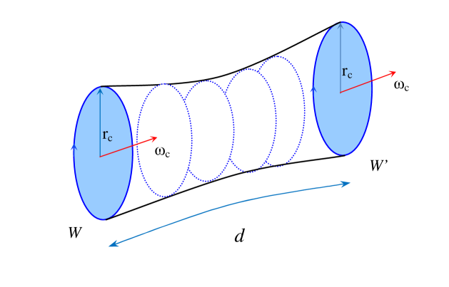
Figure 3: Correlation function for two large parallel transport loops of size $r_{c}$ and orientation $\omega_{c}$, separated by a geodesic distance $d$.

5 Renormalization Group Scaling Relations for Gravity

In this section some of the basic scaling relations for quantum gravity will be summarized. It is by now established wisdom, at least in most field theories besides gravity, that standard scaling arguments allow one to determine the scaling behavior of local averages, correlation functions and even suitable nonlocal observables such as the Wilson loop from the knowledge of the basic renormalization group behavior, and specifically from the universal critical exponents. The latter generally characterize the singular behavior of local averages in the vicinity of the critical point, a nontrivial fixed point of the renormalization group (RG) in field theory language. For extensive reviews on the subject see for example [15, 35, 16, 36, 37]. There is by now a rather well established body of knowledge in quantum field theory and statistical field theory on this subject, and there is no apparent reason why its basic tenets should not apply to gravity as well, with quantum gravity describing the unique theory of a massless spin two particle coupled to a covariantly conserved energy momentum tensor [8].

It is also understood that in the vicinity of a critical point (seen as equivalent to a nontrivial fixed point of the renormalization group) long range correlations arise due to the appearance of a massless particle. In statistical field theory language, the presence of a massless particle is reflected in a divergent correlation length $\xi=1/m$, or equivalently a power law in the relevant correlation functions. Let us summarize here the basis for the scaling assumptions for local averages, fluctuations and their correlations. In brief, since $\log Z$ in either Eq. (1) or (5) is both dimensionless and extensive, for a volume $V\sim L^{d}$ it has to have the form

$$\log\,Z(k)\;=\;f_{a}\;\left({L\over l_{0}}\right)^{d}\;+\;f_{s}\;\left({L\over\xi}\right)^{d}$$ (39)

where here $f_{a}$ and $f_{s}$ are nonsingular functions of dimensionless parameters, $\xi$ is the fundamental correlation length (the distance over which quantum fluctuations are strongly correlated), and $l_{0}\sim a$ the fundamental lattice spacing or ultraviolet cutoff. Then the free energy or generating function, defined as

$$F(k)\;=\;-{1\over V}\;\log\,Z(k)\;,$$ (40)

is expected, based on purely dimensional grounds, to aquire a singular part $F_{sing}(k)$ such that [44]

$$F_{sing}(k)\;\sim\;\xi^{-d}\;\;.$$ (41)

If one sets for the nonperturbative correlation length $\xi$

$$\xi(k)\;\;\mathrel{\mathop{\sim}_{k\rightarrow k_{c}}}\;\;A_{\xi}\;(k_{c}-k)^{-\nu}\;,$$ (42)

where $A_{\xi}$ is the correlation length amplitude, $k_{c}$ the critical point and $\nu$ the correlation length exponent characterizing the divergence of $\xi$ at the critical point, then one obtains for the singular part of the free energy

$$F_{sing}\;\;\mathrel{\mathop{\sim}_{k\rightarrow k_{c}}}\;\;(k_{c}-k)^{d\,\nu}\;.$$ (43)

One concludes that a divergent correlation length signals the presence of a phase transition, and this in turn leads to the appearance of nonanaliticities in thermodynamic quantities such as $Z(k)$ and the free energy $F(k)$. The origin of these nonanaliticities in $Z(k)$ lies therefore in the divergence of $\xi$ in the vicinity of the critical point at $k_{c}$, where the theory becomes scale invariant.

The following results then follow more or less immediately from the definitions in Eqs. (1) or (5), and in Eq. (17). Near the singularity the average curvature behaves as

$${\cal R}(k)\;\;\mathrel{\mathop{\sim}_{k\rightarrow k_{c}}}\;\;-\,A_{\cal R}\,(k_{c}-k)^{\delta}\;\;,$$ (44)

with a curvature exponent $\delta$ related to the exponent $\nu$ introduced earlier in Eq. (42) by the scaling relation $\delta\,=\,d\,\nu\,-\,1$. Consequently the presence of a phase transition can already be inferred directly from the appearance of nonanalytic terms in invariant local averages, such as the average curvature. Similarly, one has for the curvature fluctuation defined in Eq. (16), using Eqs. (18) and (42),

$$\chi_{\cal R}(k)\;\;\mathrel{\mathop{\sim}_{k\rightarrow k_{c}}}\;\;\delta\,A_{\cal R}\;(k_{c}-k)^{-(1-\delta)}\;\;\;\;.$$ (45)

Again, scaling [Eqs. (42) and (43)] relates the exponent $\delta$ appearing in the curvature fluctuation to $\nu$, so that the exponent in Eq. (45) is simply $1\,-\,\delta\;=\;2\,-\,d\,\nu$. These results show that from suitable averages one can extract the correlation length exponent $\nu$ [defined in Eq. (42)], without even a need to compute an invariant two-point function, such as the ones in Eqs. (24), (25), (26) and (27), provided scaling holds. Furthermore, in the vicinity of the critical point $k_{c}$ one can trade the distance from the critical point for the correlation length $\xi$, and obtain the following equivalent result relating the quantum expectation value of the local curvature to the physical correlation length $\xi$,

$${\cal R}(\xi)\;\;\mathrel{\mathop{\sim}_{k\rightarrow k_{c}}}\;\;\xi^{1/\nu-d}\;\;.$$ (46)

This last expression is obtained from Eqs. (42) and (44), using $\delta\,=\,d\,\nu\,-\,1$. Matching of dimensionalities here can always be achieved by supplying appropriate powers of the lattice spacing $l_{0}\sim a$ or, equivalently, the Planck length $l_{P}=\sqrt{G}$.

In addition, the above results allow one to relate the fundamental scaling exponent $\nu$ of Eq. (42) to the scaling behavior of some correlation functions at large distances. Thus, for example, the curvature fluctuation of Eq. (15) is related to the connected scalar curvature correlation of Eq. (26) evaluated at zero momentum

$$\chi_{\cal R}(k)\sim{\int d^{4}x\int d^{4}y<\sqrt{g}R(x)\,\sqrt{g}R(y)>_{c}\over<\int d^{4}x\sqrt{g}>}\;\;\mathrel{\mathop{\sim}_{k\rightarrow k_{c}}}\;\;A_{\chi}\,(k_{c}-k)^{\delta-1}\;.$$ (47)

It follows that a divergence in the curvature fluctuation is indicative of long range correlations, corresponding to the presence of a massless particle, the graviton. Close to the critical point one expects, in the scaling limit, i.e. for physical distances much larger than the fundamental lattice spacing, a power law decay in the geodesic distance $d$, as in Eq. (26),

$$<\sqrt{g}R(x)\sqrt{g}R(y)>_{c}\;\;\mathrel{\mathop{\sim}_{|x-y|\rightarrow\infty}}\;\;\frac{1}{|x-y|^{2n}}\;\;\;\;.$$ (48)

After inserting the correlation function from Eq. (48) in the expression of Eq. (47) and then integrating over a region of size $\xi$ one obtains immediately for the power in Eq. (48)

$$n\;=\;d\,-\,1/\nu\;\;.$$ (49)

Thus knowledge of the scaling exponent $\nu$ uniquely determines the power in Eqs. (48) and (26).

So, the scaling theory for gravity just outlined implies a universal relationship between various quantities and the exponents that appear in them. Of course the nonperturbative scaling exponents can be determined, in principle, separately for each individual observable. Nevertheless scaling theory, based on the assumption of the existence of a massless particle in the vicinity of an ultraviolet fixed point, immediately implies a direct (and testable) relationship between the scaling behavior of various quantities, such as the ones in Eqs. (13),(15), (26), (27) and (42). Ultimately, the physical relevance of the above results is that Eq. (42) gives, when solved for $k$ or $G$, the running of $G$ with scale in the vicinity of the fixed point at $G_{c}$. Thus, again, Eqs.(44) and (45) are useful for an accurate determination of the universal scaling exponent $\nu$, and this quantity in turn determines the scaling behavior of invariant curvature correlation functions in Eqs. (26) and (48) as a function of geodesic distance.

6 Continuum Limit of Lattice Quantum Gravity

The long distance behavior of quantum field theories is, to a great extent, determined by the scaling behavior of the relevant coupling constants under a change in momentum scale. Asymptotically free theories such as QCD lead to vanishing gauge couplings at short distances, while the opposite is true for QED. In general the fixed point(s) of the renormalization group need not be at zero coupling, but can be located at some finite $G_{c}$, leading to nontrivial fixed points or more complex limit cycles [2, 4, 41, 16].

These general ideas are realized concretely in the analytic $2+\epsilon$ expansion for gravity, and reappear later in essentially the same form in lattice gravity in four dimensions. In the $2+\epsilon$ perturbative expansion for gravity [20, 21, 22, 23] one analytically continues in the spacetime dimension using dimensional regularization, and applies perturbation theory about $d=2$, where Newton’s constant becomes dimensionless. A similar method is quite successful in determining the critical properties of the $O(n)$-symmetric nonlinear sigma model above two dimensions [45]. In the framework of this expansion the dimensionful bare coupling is written as $G_{0}=\Lambda^{2-d}\,G$, where $\Lambda$ is an ultraviolet cutoff (corresponding on the lattice to a momentum cutoff comparable to the inverse average lattice spacing, $\Lambda\sim 1/l_{0}\sim 1/a$). There were originally some known technical difficulties with this expansion due to the presence of kinematic singularities for the graviton propagator in two dimension (the Einstein action is a topological invariant in $d=2$), but these have been overcome recently. In addition, one can show that a gauge-choice dependent renormalization of the bare cosmological constant $\lambda_{0}$ can be completely reabsorbed into an overall rescaling of the metric, with no physical consequences. A double expansion in $G$ and $\epsilon=d-2$ then leads in lowest order to a gauge-independent nontrivial fixed point in $G$ above two dimensions

$$\beta(G)\,\equiv\,{\partial G\over\partial\log\Lambda}\,=\,(d-2)\,G\,-\,\beta_{0}\,G^{2}\,+\cdots\;\;,$$ (50)

with $\beta_{0}>0$ for pure gravity. To lowest order the ultraviolet fixed point is then at $G_{c}\,=\,1/\beta_{0}(d-2)$. Integrating Eq. (50) close to the nontrivial fixed point one obtains for $G>G_{c}$

$$m_{0}\,=\,\Lambda\,\exp\left({-\int^{G}\,{dG^{\prime}\over\beta(G^{\prime})}}\right)\;\;\mathrel{\mathop{\sim}_{G\rightarrow G_{c}}}\;\;\Lambda\,|\,G-G_{c}\,|^{-1/\beta^{\prime}(G_{c})}\;\;\;\;,$$ (51)

where $m_{0}$ an integration constant, with dimensions of a mass or inverse length, expected to be associated with some physical scale. It is rather natural here to identify this scale with the inverse of the gravitational correlation length ($\xi=m^{-1}$), or some equivalent scale associated with the physical large-scale curvature [28, 29]. Note that the derivative of the beta function at the fixed point defines the critical exponent $\nu$, which to this order is independent of $\beta_{0}$, $\beta^{\prime}(G_{c})\,=\,-(d-2)\,=\,-1/\nu$.

The previous results clearly illustrate how the lattice continuum limit should be taken. It corresponds to $\Lambda\rightarrow\infty$, $G\rightarrow G_{c}$ with the physical scale $\xi=1/m$ held constant; thus for fixed lattice cutoff the continuum limit is approached by tuning $G$ to $G_{c}$. In four dimensions the universal critical exponent $\nu$ is defined by [see Eq. (42)]

$$\xi^{-1}(G)\,\equiv\,m(G)\;\;\mathrel{\mathop{\sim}_{G\rightarrow G_{c}}}\;\;A_{m}\,\Lambda\,|\,G(\Lambda)-G_{c}|^{\nu}\;\;,$$ (52)

where $\Lambda=1/a$ is the inverse lattice spacing, and the nonperturbative mass scale $m=1/\xi$ is defined as the inverse of the correlation length, with $A_{m}$ a nonperturbative but calculable amplitude. The cutoff independence of the nonperturbative mass scale $m$ implies

$$\Lambda\,{d\over d\,\Lambda}\,m(\Lambda,G(\Lambda))\;=\;0\;\;.$$ (53)

Comparing results in Eqs. (51) and (52) one obtains

$$\beta^{\prime}(G_{c})\,=\,-1/\nu\;\;,$$ (54)

so that the universal exponent $\nu$ is directly related to the derivative of the Callan-Symanzik $\beta$ function for $G$ in the vicinity of the ultraviolet fixed point. Thus computing $\nu$ is equivalent to computing the universal derivative of the beta function at $G_{c}$.

It is easy to see here that the value of $\nu$ determines the running of the effective coupling $G(\mu)$ in the vicinity of the fixed point, where $\mu$ is an arbitrary momentum scale. The renormalization group tells us that in general the effective coupling will grow or decrease with length scale $r=1/\mu$, depending on whether $G>G_{c}$ or $G<G_{c}$, respectively. This result follows from the fact that the genuinely nonperturbative physical mass parameter $m=\xi^{-1}$ is itself scale independent, and obeys therefore the rather simple Callan-Symanzik renormalization group equation

$$\mu\;{d\over d\,\mu}\;m(\mu,G(\mu))\;\equiv\;\mu\;{d\over d\,\mu}\;\left\{\;A_{m}\,\mu\;|\,G(\mu)-G_{c}|^{\nu}\;\right\}\,=\,0\;\;\;\;.$$ (55)

Here again, by virtue of Eq. (52), the second expression on the right-hand-side is appropriate in the vicinity of the ultraviolet fixed point at $G_{c}$. Nevertheless the above discussion is not necessarily limited to just a region in the immediate vicinity of $G_{c}$; more generally, if one defines the function $F(G)$ via

$$\xi^{-1}\;\equiv\;m\;=\;\Lambda\;F(G(\Lambda))\;\;,$$ (56)

then, from the usual definition of the Callan-Symanzik $\beta$ function $\beta(G)\,=\,\partial G(\Lambda)/\partial\log\Lambda$, one obtains

$$\beta(G)\;=\;-\,{F(G)\over F^{\prime}(G)}\;\;,$$ (57)

which shows that the renormalization group $\beta$-function, and thus the running of $G(\mu)$ with scale, can be defined also some distance away from the nontrivial ultraviolet fixed point [including therefore the higher order corrections in Eq. (55)]. So, more generally, the running of $G(\mu)$ is obtained by solving the differential equation

$$\mu\;{d\,G(\mu)\over d\,\mu}\,=\,\beta(G(\mu))\;,$$ (58)

with $\beta(G)$ obtained from Eq. (57). It is then clear from the previous discussion that the physical mass scale $m=\xi^{-1}$ determines the magnitude of the scaling corrections, and plays a role similar to the scaling violation parameter $\Lambda_{\overline{MS}}$ in QCD (as in gauge theories, this nonperturbative mass scale emerges in spite of the fact that the fundamental gauge boson remains strictly massless to all orders in perturbation theory, and consequently does not violate local gauge invariance). Furthermore, as in gauge theories, one expects in gravity that the magnitude of $\xi$ cannot be determined perturbatively, and to pin down its value requires a fully nonperturbative approach such as the lattice formulation.

Solving explicitly Eq. (55) for $G(q^{2})$, with $q$ an arbitrary wavevector scale, one obtains

$$G(q^{2})\;=\;G_{c}\left[\;1\,+\,c_{0}\,\left({m^{2}\over q^{2}}\right)^{1/2\,\nu}\,+\,O(\left({m^{2}\over q^{2}}\right)^{1/\nu})\;\right]\;\;.$$ (59)

Here the amplitude of the quantum correction $c_{0}$ is directly related to the constant $A_{m}$ in Eq. (52) by

$$c_{0}\;\equiv\;{1\over G_{c}\,A_{m}^{1/\nu}}\;\;.$$ (60)

One important point is that the magnitude of the quantum correction in Eq. (59) depends crucially on the magnitude of the nonperturbative physical scale $\xi$. Also, the expression in Eq. (59) does not satisfy general covariance; this in turn can be fixed by performing the replacement $q^{2}\rightarrow-\Box$ where $\Box(g_{\mu\nu})$ is the covariant D’Alembertian for a given background metric $g_{\mu\nu}(x)$ [46]. This then leads, from Eq. (59), to

$$G(\Box)\;=\;G_{c}\left[\;1\,+\,c_{0}\,\left({1\over-\xi^{2}\,\Box^{2}}\right)^{1/2\,\nu}\,+\,\dots\;\right]\;\;.$$ (61)

A set of manifestly covariant effective field equations with a $G(\Box)$ takes the simple form [46]

$$R_{\mu\nu}\,-\,\textstyle{1\over 2}\displaystyle\,g_{\mu\nu}\,R\,+\,\lambda\,g_{\mu\nu}\;=\;8\pi\,G(\Box)\,T_{\mu\nu}\;\;$$ (62)

with the nonlocal contribution coming from the quantum correction in the $G(\Box)$ of Eq. (61). These nonlocal effective field equations can then be solved for a number of physically relevant metrics. For the specific case of a static isotropic metric it is possible to obtain an exact expression for $G(r)$ in the limit $r\gg 2MG$ [46]. The result, for $\nu=1/3$ exactly, reads

$$G\;\rightarrow\;G(r)\;=\;G\,\left(1\,+\,{c_{0}\over 3\,\pi}\,m^{3}\,r^{3}\,\ln\,{1\over m^{2}\,r^{2}}\,+\,\dots\right)$$ (63)

with $m=1/\xi$. This last result is vaguely reminiscent of the Uehling (vacuum polarization) correction to the static potential found in QED. Generally the expressions in Eqs. (59), (61) and (63) are consistent with a gradual slow increase in $G$ with large distance $r$, and with a modified Newtonian potential in the same limit.

The remainder of this paper will deal therefore with establishing firm values for the nonperturbative amplitudes and exponents defined in the previous sections, and later determining both qualitatively and quantitatively their effects on the running of Newton’s $G$ and on the long distance behavior of physical correlation functions, such as the ones defined in the previous sections.

7 Average Local Curvature

Next we come to a discussion of the numerical methods employed in this work and the analysis of the results. For the reader who is not interested in such details, a separate section later summarizes the most important results obtained so far. As in previous work, the edge lengths are updated by a Monte Carlo algorithm, generating eventually an ensemble of configurations distributed according to the action and measure of Eq. (5). Details of the method as it applies to pure gravity are discussed in [14, 48], and will not be repeated here.

In this work lattices of size $L^{4}$ with $L=4$ (256 sites, 3,840 edges and 6,144 simplices), $L=8$ (4,096 sites, 61,440 edges and 98,304 simplices), $L=16$ (65,536 sites, 983,040 edges and 1,572,864 simplices), $L=32$ (1,048,576 sites, 15,728,640 edges and 25,165,824 simplices), and $L=64$ (16,777,216 sites, 251,658,240 edges and 402,653,184 simplices) have been considered. These lattices are all constructed by conveniently dividing up hypercubes into simplice by introducing suitable diagonals [18], and periodic boundary conditions are used throughout. In general for a lattice with $L^{4}$ sites one has $15$ edges per vertex and $24$ four-simplices per vertex. For these lattices one should keep in mind that due to the simplicial nature of the lattice there are many edges per hypercube with many interaction terms; as a consequence the statistical fluctuations already for one single hypercube can be comparatively small, unless one is very close to a critical point. The results presented here are still preliminary, and in the future it should be possible to repeat such calculations with improved accuracy on even larger lattices. Also, while the overall statistics on the $32^{4}$ lattice seems adequate, the overall statistics on the $64^{4}$ lattices was yet far too low to be usable in the present analysis.

On the $32^{4}$ lattice up to 200,000 consecutive configurations were generated for each value of $k$, and 9 different values for the parameter $k$ were chosen. On the $16^{4}$ lattice up to 800,000 consecutive configurations were generated for each value of $k$, and 32 different values for $k$ were chosen. In addition, results for different values of $k$ can be considered as completely statistically uncorrelated, since they originated from unrelated edge length configurations. On the smaller $8^{4}$ lattice 200,000 consecutive configurations were generated for each value of $k$. On the $4^{4}$ lattice two million consecutive configurations were generated for each value of $k$. To accumulate enough statistics, runs were performed around the clock on a 1200 core machine over a period of roughly four months. As a result, the increase in accuracy is significant compared to the results presented in previous work done at the time on a dedicated 32-node cluster [48].

In this work the topology is restricted to a four-torus (periodic boundary conditions). One could perform similar calculations with other lattices employing different boundary conditions or topology, but one expects that the universal long distance scaling properties of the theory to be determined by short-distance renormalization effects, which are generally independent of the boundary conditions at infinity. A clear example of this is of course the Feynman diagrammatic expansion for gravity in $2+\epsilon$ dimensions, where boundary conditions play no role in the renormalization of the couplings. In addition, it will be necessary to impose, based on physical considerations, the constraint that the correlation length in lattice units be much larger than the average lattice spacing, and at the same time much smaller than the overall linear size of the system, $l_{0}\;\mathrel{\hbox to0.0pt{\lower 4.0pt\hbox{\hskip 1.0pt$\sim$}\hss}\raise 1.0pt\hbox{$<$}}\;\xi\;\mathrel{\hbox to0.0pt{\lower 4.0pt\hbox{\hskip 1.0pt$\sim$}\hss}\raise 1.0pt\hbox{$<$}}\;L_{0}$, where $L_{0}\sim V^{1/4}$ here is the linear size of the system, and $l_{0}\sim a$ the (average) lattice spacing.

As stated earlier, the bare cosmological constant $\lambda_{0}$ appearing in the gravitational action of Eq. (5) is set $1$ since its value just sets the overall length scale in the problem. The higher derivative coupling $a_{0}$ was also set to $0$ (pure Regge-Einstein action). It is possible to introduce $R^{2}$-type terms in the action, nevertheless in this work these terms were not included in order not to “contaminate” the results with the effects of such higher derivative terms. These terms were studied extensively in [48], and their effects is generally to stabilize the theory at the expense of nonunitary contributions, which cause a visible oscillatory behavior in curvature correlations at short distances. The downside of not including any lattice higher derivative terms is that the theory eventually develops instabilities very close to the critical point in $G$, which need to be handled properly by an extrapolation or analytic continuation in $G$. Nevertheless, as has been shown in [48] and in the discussion further below, such an extrapolation or analytic continuation is fairly unambiguous, given a large enough amount of high precision numerical data. Indeed such an instability is in fact expected on the basis of the well-known Euclidean conformal mode contribution, arising from a kinetic energy contribution for the conformal mode with the wrong sign [11, 12]. Its appearance should therefore be regarded as consistent with the full recovery of a continuum behavior in the vicinity of the ultraviolet fixed point at $G_{c}$.

For the measure in Eq. (5) the above choice of parameters then leads to a well behaved ground state for $k<k_{c}\approx 0.052$ for $a=0$ [48, 49]. Given this choice of parameters the system then resides in the ‘smooth’ phase, with a fractal dimension close to four; on the other hand for $k>k_{c}$ the local curvature can become rather large (‘rough’ phase), and lattice spacetime collapses into a degenerate configuration with very long, elongated simplices and thus more akin to a two-dimensional lattice [14, 19, 49, 48].

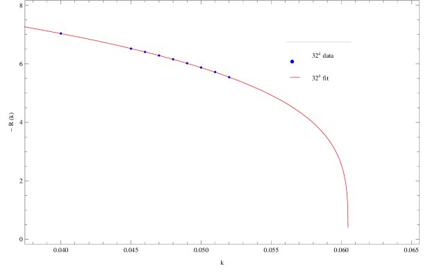
Figure 5: Average local curvature ${\cal R}(k)$ as defined in Eq. (14), computed on a large lattice with $32^{4}=1,048,576$ sites. Note the change in horizontal scale as compared to the previous figure. Statistical errors ($\sim{\cal O}(10^{-4})$) are much smaller than the size of the symbols. The continuous line represents a fit of the form $A\;(k_{c}-k)^{\delta}$ for $k\geq 0.04$, with exponent $\delta=4\nu-1$ .

The results obtained for the average curvature ${\cal R}$ [defined in Eq. (14)] as a function of the bare coupling $k$ are shown in Figures 4 to 8, on lattices of increasing size with $4^{4}$, $8^{4}$, $16^{4}$ and $32^{4}$ sites. Figures 5 and 7 show the $32^{4}$ data by itself. The errors there are quite small, of the order of a tenth of a percent or less, and are therefore not visible in the graph. In [48] it was found that as $k$ is varied, the average local curvature is negative for sufficiently small $k$ (’smooth’ phase), and appears to go to zero continuously at some finite value $k_{c}$. For $k\geq k_{c}$ the curvature becomes very large, and the simplices tend to collapse into degenerate configurations with very small volumes ($<\!V\!>/<\!l^{2}\!>^{2}\;\sim 0$). This collapsed phase corresponds to the region of the usual weak field expansion ($G\sim 0$), characterized by unbounded fluctuations in the conformal mode.

Accurate and reproducible curvature data can only be obtained for $k$ below the instability point $k_{u}$ since, as already pointed out in [48], for $k>k_{u}\approx 0.052$ an instability develops, presumably associated with the unbounded conformal mode. Its signature is typical of a sharp first order transition, beyond which the system tunnels into the rough, elongated phase which is two-dimensional in nature with no physically acceptable continuum limit. This instability is caused by the appearance of one or more localized singular configuration, with a spike-like curvature singularity, and is clearly driven by the Euclidean Einstein term in the action, and in particular its unbounded conformal mode contribution. Nevertheless an important result that emerges from the lattice calculations is that for sufficiently strong coupling such singular configurations are suppressed by quantum fluctuations and thus by the nature of the measure, which imposes nontrivial constraints coming from the generalized triangle inequalities. The lattice results suggest therefore that the conformal instability is entirely cured for sufficiently strong coupling. It is characteristic of first order transitions that the free energy develops an infinitely sharp delta-function singularity at $k_{u}$, with the metastable branch developing no nonanalytic contribution at $k_{u}$. Indeed it is well known from the theory of first order transitions that tunneling effects will lead to a purely imaginary contribution to the free energy, with an essential singularity for $k>k_{u}$ [15]. In the following we shall therefore clearly distinguish the instability point $k_{u}$ from the true critical point at $k_{c}$. Consequently the nonanalytic behavior of the free energy (and its derivatives which include, for example, the average curvature) has to be obtained by analytic continuation of the Euclidean theory into the metastable branch. This procedure is then formally equivalent to the construction of the continuum theory exclusively from its strong coupling (small $k$ or large $G$) expansion, for example starting from

$$Z_{L}(k)\;=\;\sum_{n=0}^{\infty}a_{n}k^{n}\;\;,$$ (64)

$${\cal R}(k)\;=\;\sum_{n=0}^{\infty}b_{n}k^{n}\;\;,$$ (65)

$$\chi_{\cal R}(k)\;=\;\sum_{n=0}^{\infty}c_{n}k^{n}\;\;.$$ (66)

Given a large enough number of terms in this expansion, the nonanalytic behavior in the vicinity of the true critical point at $k_{c}$ can then be determined unambiguously, using for example differential or Pade approximants [50, 51] for suitable combinations which are expected to be meromorphic in the vicinity of the true critical point. In the present case, instead of the analytic strong coupling expansion, one makes use of a set of (in principle, arbitrarily) accurate data points to which the expected functional form can be fitted. What is assumed here then is the kind of regularity which is always assumed in extrapolating finite series to the boundary of their radius of convergence. Ultimately it should be kept in mind though that one is really interested in the pseudo-Riemannian case, and not the Euclidean one for which such an instability due to the conformal mode is, as stated before, to be expected. Indeed had such an instability not occurred one might wonder if the resulting theory still had any relationship to the original continuum theory: for the lattice theory one expects such an instability to develop at some point, since the continuum theory is known to be unstable for weak enough coupling. In conclusion, in the following only data for $k\leq k_{u}$ will be considered; in fact to add a margin of safety only $k\leq 0.051$ will be considered throughout the rest of the paper.

To extract the critical exponent $\delta$, one fits the computed values for the average curvature to the form of Eq. (44). It would seem unreasonable to expect that the computed values for ${\cal R}$ are accurately described by this function even for small $k$, away from the critical point at $k_{c}$. Instead, the data is fitted to the above functional form for either $k\geq 0.02$ or $k\geq 0.03$. Then the difference in the fit parameters can be used as one more measure for the error. In addition, it is possible to include a subleading correction of the form

$${\cal R}(k)\;\;\mathrel{\mathop{\sim}_{k\rightarrow k_{c}}}\;\;-A_{\cal R}\,\left[\;k_{c}-k+B\;(k_{c}-k)^{2}\;\right]^{\delta}\;\;\;\;,$$ (67)

and use the results to further constraint the uncertainties in the amplitude $A_{\cal R}$, $k_{c}$ and the exponent $\delta=4\nu-1$. Using this set of procedures for ${\cal R}(k)$ one obtains on a lattice with $L^{4}$ sites the following set of estimates

$$L=4\;\;\;\;k_{c}=0.07025(20)\;\;\;\;\;\nu=0.357(8)$$ (68)

$$L=8\;\;\;\;k_{c}=0.05811(27)\;\;\;\;\;\nu=0.308(16)$$ (69)

$$L=16\;\;\;\;k_{c}=0.06134(11)\;\;\;\;\;\nu=0.322(6)$$ (70)

$$L=32\;\;\;\;k_{c}=0.06094(10)\;\;\;\;\;\nu=0.320(6)\;\;.$$ (71)

Then using the same set of procedures for $|{\cal R}(k)|^{3}$ (which assumes $\nu=1/3$ exactly) one obtains on the same $L^{4}$ lattices

$$L=4\;\;\;\;k_{c}=0.06485(20)$$ (72)

$$L=8\;\;\;\;k_{c}=0.06337(27)$$ (73)

$$L=16\;\;\;\;k_{c}=0.06377(11)$$ (74)

$$L=32\;\;\;\;k_{c}=0.06387(9)\;\;.$$ (75)

This last result is presumably the most accurate one, since it is derived form the largest lattice, with the highest statistics and the smallest errors on the individual data points. All of these results are displayed in Figures 4 to 8, and indicate that the exponent $\nu$ (and therefore $\delta$) is indeed very close to $1/3$. Specifically, Figures 6,7 and 8 show a graph of the average curvature ${\cal R}(k)$ raised to the third power; one would expect to get a straight line close to the critical point if the exponent for ${\cal R}(k)$ is exactly $1/3$. The numerical results indeed support such an assumption, and the linearity of the results close to $k_{c}$ is quite striking. The computed data is quite close to a straight line over a wide range of $k$ values, providing further support for the assumption of an algebraic singularity for ${\cal R}(k)$ itself, with exponent close to $1/3$. This last value can be compared to the old estimate computed in [48], $\nu\approx 0.33$.

Figure 4: Average local curvature ${\cal R}(k)$ as defined in Eq. (14), computed on a lattice with $16^{4}=65,536$ sites. Statistical errors ($\sim{\cal O}(10^{-4})$) are much smaller than the size of the symbols. The continuous line represents a fit of the form $A\;(k_{c}-k)^{\delta}$ for $k\geq 0.02$, with exponent $\delta=4\nu-1$ .

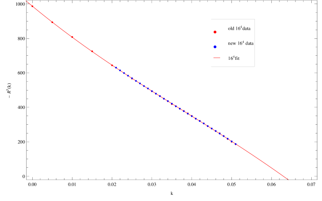
Figure 6: Average local curvature ${\cal R}(k)$ on the $16^{4}$ lattice, raised to the third power. If $\delta=\nu=1/3$ exactly, then all the data should fall on a straight line close to $k_{c}$. The continuous line here represents a linear fit of the form $A\;(k_{c}-k)$ for $k\geq 0.02$. Deviations from linearity of the transformed data are rather small.

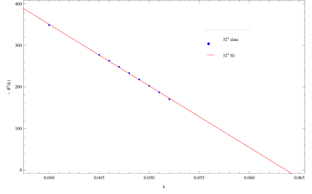
Figure 7: Average local curvature ${\cal R}(k)$ on the larger $32^{4}$ ($1,048,576$ sites) lattice, raised to the third power. Again if $\delta=\nu=1/3$ exactly, then the points should all fall on a straight line. The continuous line represents a linear fit of the form $A\;(k_{c}-k)$. Deviations from linearity of the transformed data are rather small.

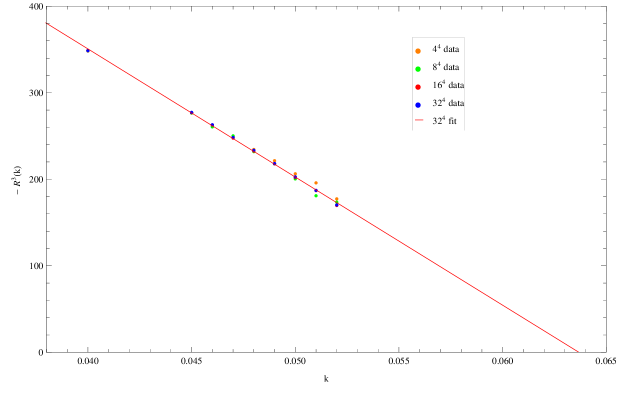
Figure 8: Volume dependence of the average local curvature $|{\cal R}(k)|^{3}$ on lattices with $4^{4}$, $8^{4}$, $16^{4}$ and $32^{4}$ sites. Again, if $\delta=\nu=1/3$ exactly, then the data should all fall on a straight line close to $k_{c}$. The continuous line represents a linear fit of the form $A\;(k_{c}-k)$. The size dependence becomes rather small on the larger lattices, unless one moves very close to the critical point.

8 Curvature Fluctutations

Figures 9 to 12 show the average curvature fluctuation $\chi_{\cal R}(k)$ defined in Eq. (16). At the critical point the curvature fluctuation is expected to diverge, by definition. As in the case of the average local curvature ${\cal R}(k)$ analyzed previously, one can extract the critical exponent $\delta$ and $k_{c}$ by fitting the computed values for the curvature fluctuation to the form given in Eq. (45). And, as for the average curvature itself, it would seem unreasonable to expect that the computed values for $\chi_{\cal R}(k)$ are accurately described by this function even for small $k$, away from the critical point. Instead the data has been fitted to the above functional form either for $k\geq 0.02$ or for $k\geq 0.03$, and the difference in the fit parameters is then used as a measure for the error. In addition one can include here a subleading correction as well, of the form

$$\chi_{\cal R}(k)\;\;\mathrel{\mathop{\sim}_{k\rightarrow k_{c}}}\;\;-A_{\chi_{\cal R}}\left[\;k_{c}-k+B(k_{c}-k)^{2}\;\right]^{-(1-\delta)}\;\;\;\;,$$ (76)

and use the results to further constraint the errors on the amplitude $A_{\chi_{\cal R}}$, $k_{c}$ and the exponent $\delta=4\nu-1$.

One finds that the values for $\delta$ and $k_{c}$ obtained in this fashion are consistent with the ones obtained from the average curvature ${\cal R}(k)$, but here with somewhat larger errors, since fluctuations are notoriously more difficult to compute accurately than local averages, and require therefore significantly higher statistics. Using these procedures one obtains on the largest lattices with $16^{4}$ and $32^{4}$ sites

$$k_{c}=0.05383(102)\;\;\;\;\;\nu=0.350(56)\;\;\;\;.$$ (77)

Alternatively, one can use for $\chi_{\cal R}(k)$ the best estimate for $k_{c}$ obtained earlier from the average curvature. This then gives

$$\nu=0.321(12)\;\;\;\;,$$ (78)

which is closer to the value obtained from ${\cal R}(k)$.

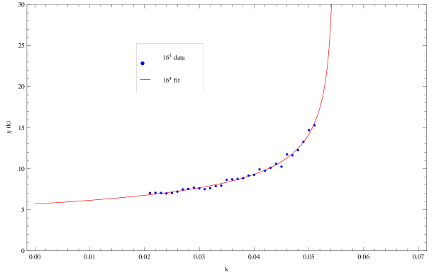
Figure 9: Curvature fluctuation $\chi_{\cal R}(k)$ on lattices with $16^{4}=65,536$ sites. The continuous line represents a fit of the form $\chi_{\cal R}(k)\;=\;A\;(k_{c}-k)^{-(1-\delta)}$ for $k\geq 0.02$.

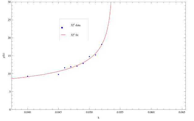
Figure 10: Curvature fluctuation $\chi_{\cal R}(k)$ on the $32^{4}$ lattice with $1,048,576$ sites. Note the change in scale from the previous figure. The line shown is a best fit of the form $\chi_{\cal R}(k)\;=\;A\;(k_{c}-k)^{-(1-\delta)}$ for $k\geq 0.04$.

Figures 11 and 12 show the inverse curvature fluctuation $\chi_{\cal R}(k)$ on the $16^{4}$ and $32^{4}$-site lattices, raised to power $3/2$. One would expect to get a straight line close to the critical point if the exponent for $\chi_{\cal R}(k)$ is exactly $-2/3$. The computed data is more or less consistent with a linear behavior for $k\geq 0.03$, providing further support for an algebraic singularity for $\chi_{\cal R}(k)$ itself, with exponent close to $-2/3$. Using this last procedure one finds on the largest ($16^{4}$ and $32^{4}$) lattices the improved estimate for the critical point

$$k_{c}=0.06369(84)\;\;\;\;,$$ (79)

which is consistent with the value obtained earlier from ${\cal R}^{3}$ (see Figures 6 to 8 and related discussion), and suggests again that the exponent $\nu$ must be rather close to $1/3$.

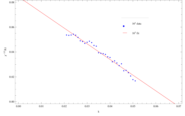
Figure 11: Inverse curvature fluctuation raised to the power $3/2$, on the $16^{4}$ lattice; note that the data is scaled by a factor of $\times 100$. The straight line represents a linear fit of the form $A\;(k_{c}-k)$. The location of the critical point in $k$ is consistent with the estimate obtained from the average curvature, but with a somewhat larger error.

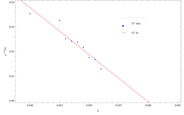
Figure 12: Inverse curvature fluctuation raised to the power $3/2$, on the $32^{4}$ lattice; note that the data is scaled by a factor of $\times 100$. The straight line represents a linear fit of the form $A\;(k_{c}-k)$. The location of the critical point in $k$ is consistent with the estimate obtained from the average curvature on the same size lattice, here with a larger uncertainty.

In order to check the consistency of the results so far, it is possible to analyze the previous calculations in a different way. From the definition of the average curvature ${\cal R}$ and curvature fluctuation [Eqs. (14) and (16)], and the fact that they are both proportional to derivatives of the free energy $F$ with respect to $k$ [Eqs. (17) and (18)], one notices that their ratio is given by

$${2\langle l^{2}\rangle\;\chi_{\cal R}(k)\over{\cal R}(k)}\;\sim\;(\frac{\partial}{\partial k}\ln Z_{L})\,/\,(\frac{\partial^{2}}{\partial k^{2}}\ln Z_{L})\;\sim\;\frac{\partial}{\partial k}\ln\left(\frac{\partial}{\partial k}\ln Z_{L}\right)\;\;.$$ (80)

The assumption of an algebraic singularity in $k$ for ${\cal R}$ and $\chi_{\cal R}$ (Eqs. (44) and (45)) then implies that the logarithmic derivative as defined above has a simple pole at $k_{c}$, with residue $\delta=4\nu-1$

$${2\langle l^{2}\rangle\;\chi_{\cal R}(k)\over{\cal R}(k)}\;\;\mathrel{\mathop{\sim}_{k\rightarrow k_{c}}}\;\;{\delta\over k-k_{c}}\;\;\;\;,$$ (81)

and the critical amplitudes dropping out entirely for this particular ratio. Figures 13 and 14 show the results for the logarithmic derivative of the average curvature ${\cal R}(k)$, obtained from the data shown earlier in Figures 4 to 12. Using this method on the largest $16^{4}$ and $32^{4}$ lattices one finds

$$k_{c}=0.06338(55)\;\;\;\;\;\nu=0.3356(84)\;\;\;\;.$$ (82)

Note that for the quantity in Eq. (81) only two parameters are fitted, as opposed to three earlier, which leads to a slightly improved accuracy. It is encouraging that the above estimates are in good agreement with the values obtained previously using the other methods.

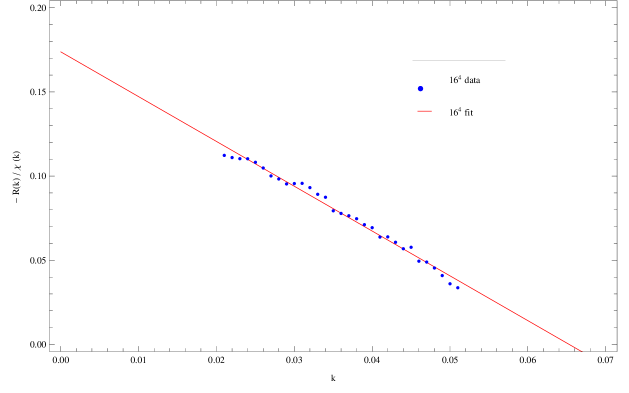
Figure 13: Inverse of the logarithmic derivative of the average curvature ${\cal R}(k)$ [defined in Eq. (81)] on the $16^{4}$ lattice with with $65,536$ sites. The straight line represents a best fit of the form $A\;(k_{c}-k)$ for $k\geq 0.02$. The location of the critical point in $k$ is consistent with the earlier estimate coming from the average curvature ${\cal R}(k)$ and its fluctuation $\chi_{\cal R}(k)$. From the slope of the line one then computes directly the exponent $\nu$.

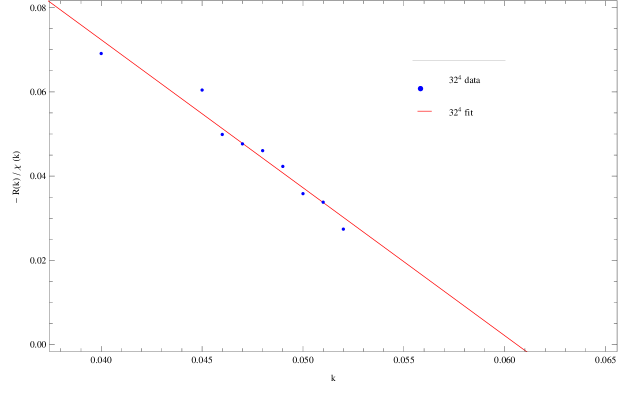
Figure 14: Inverse of the logarithmic derivative of the average curvature ${\cal R}(k)$ [defined in Eq. (81)] on the $32^{4}$ lattice with with $1,048,576$ sites. The straight line represents a best fit of the form $A\;(k_{c}-k)$ for $k\geq 0.04$. The location of the critical point in $k$ is consistent with the estimate coming from the average curvature ${\cal R}(k)$ and its fluctuation $\chi_{\cal R}(k)$. From the slope of the line one computes directly the exponent $\nu$.

As a further check, it is possible to look at the behavior of quantities when compared directly to the average local curvature. Figure 15 shows a plot of the curvature fluctuation $\chi_{\cal R}(k)$ versus the curvature ${\cal R}(k)$ (as opposed to $k$). If the average local curvature approaches zero at the critical point (where curvature fluctuation diverges), then one would expect these curvature fluctuations to diverge precisely at ${\cal R}=0$. One has from Eqs. (44) and (45)

$$\chi_{\cal R}({\cal R})\;\;\mathrel{\mathop{\sim}_{k\rightarrow k_{c}}}\;\;A\;|{\cal R}|^{(1-\delta)/\delta}\;\sim\;A\;|{\cal R}|^{(4\nu-2)/(4\nu-1)}\;\;\;.$$ (83)

An advantage of this particular combination is that it does not require the knowledge of $k_{c}$ in order to estimate $\nu$. Consequently only two parameters are fitted, the overall amplitude and the exponent in Eq. (83). Using this method one finds, assuming that the fluctuations diverge at ${\cal R}=0$,

$$\nu=0.3322(71)\;\;\;\;,$$ (84)

which is rather consistent with previous estimates. Again the error on $\nu$ can be obtained, for example, by reverting to more elaborate fits of the type

$$\chi_{\cal R}({\cal R})\;\;\mathrel{\mathop{\sim}_{{\cal R}\rightarrow 0}}\;\;A\;|\;{\cal R}+B\,{\cal R}^{2}\;|^{(4\nu-2)/(4\nu-1)}\;\;\;.$$ (85)

Note also that for $\nu=1/3$ the exponent simplifies to $-2$, and one obtains the simple result (see also Figure 15)

$$\chi_{\cal R}({\cal R})\;\;\mathrel{\mathop{\sim}_{{\cal R}\rightarrow 0}}\;\;A\;|{\cal R}|^{-2}\;\;\;.$$ (86)

One concludes that the evidence so far supports a vanishing average local curvature at the critical point, where the curvature fluctuation $\chi_{\cal R}$ and thus the correlation length $\xi$ [in view of Eqs. (45) and (42)] diverge. These results also show some degree of consistency in the values for $k_{c}$ obtained independently from ${\cal R}(k)$ and $\chi_{\cal R}(k)$ (Figures 4 to 15).

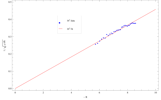
Figure 15: Inverse curvature fluctuation, $1/\sqrt{\chi_{\cal R}}$, versus the average curvature ${\cal R}$. Points shown here are for the largest lattices. For $\nu=1/3$ exactly, $1/\sqrt{\chi_{\cal R}}$ is expected to be linear in ${\cal R}$ for small ${\cal R}$.

9 Finite Size Scaling Analysis

A further consistency check on the values of the critical exponents is provided by a systematic finite size scaling (FSS) analysis. Indeed the numerical results presented in the previous sections have been obtained separately for each lattices of different size. It would be highly desirable if all those results could be combined into a single large dataset which then encompasses all the different lattice sizes, with consequently a much higher statistical significance.

Quite in general, the FSS scaling form for a quantity $O$ diverging like $t^{-x_{O}}$ in the infinite volume limit is

$$O(L,t)\;=\;L^{x_{O}/\nu}\;\left[\tilde{f_{O}}\left({L\over\xi(\infty,t)}\right)\;+\;{\cal O}(\xi^{-\omega},L^{-\omega})\right]\;\;\;,$$ (87)

with $L$ the linear size of the system, $t$ the reduced temperature or distance from the critical point, $\tilde{f_{O}}$ a smooth scaling function, $\xi(\infty,t)$ the infinite volume correlation length and $\omega$ a correction to scaling exponent; but for sufficiently large volumes the correction to scaling term involving $\omega$ can be safely neglected. In the gravity case one has $t\sim|k_{c}-k|$, and $O(L,t)$ is some physical average such as the local curvature ${\cal R}(k)$ or its fluctuation $\chi_{\cal R}(k)$, with the linear size of the system $L\sim<V>^{1/d}$ . General properties of the scaling function $\tilde{f_{O}}(y)$ include the fact that it is expected to show a peak if the finite volume value for $O$ is peaked, it is analytic at $x=0$ since no singularity can develop in a finite volume, and $\tilde{f_{O}}(y)\sim\tilde{y}^{-x_{O}}$ for large $y$ for a quantity $O$ which diverges as $t^{-x_{O}}$ in the infinite volume limit.

The expression in Eq. (87) is only useful when the infinite-volume correlation length $\xi$ is accurately known. Nevertheless close to the critical point one can use $\xi\sim t^{-\nu}$ and then deduce from it the equivalent scaling from

$$O(L,t)\;=\;L^{x_{O}/\nu}\;\left[\,\tilde{f_{O}}\left(L\;t^{\nu}\right)\;+\;{\cal O}(L^{-\omega})\,\right]\;\;\;,$$ (88)

which relies on a knowledge of $t$, and thus of the critical point, instead.

The finite size scaling behavior of the average local curvature, as defined in Eqs. (13) and (14) will be discussed next. If scaling involving $k$ and $L$ holds according to Eq. (88), with $x_{O}=1-4\nu$ the scaling dimension for the curvature, then all points for different $k$’s and $L$’s should lie on the same universal curve. From Eq. (88), with $t\sim k_{c}-k$ and $x_{O}=-\delta=1-4\nu$, one has

$${\cal R}(k,L)\;=\;L^{-(4-1/\nu)}\;\left[\;\tilde{{\cal R}}\left((k_{c}-k)\;L^{1/\nu}\right)\;+\;{\cal O}(L^{-\omega})\;\right]$$ (89)

where again $\omega>0$ is a correction-to-scaling exponent. The above argument then suggests that the quantities

$${\cal R}(k,L)\cdot L^{4-1/\nu}\;\sim\;\left(L\over\xi\right)^{4-1/\nu}$$ (90)

should all lie on a single universal curve when displayed as a function of the scaling variable

$$x\;\equiv\;(k_{c}-k)\;L^{1/\nu}\;\sim\;\left(L\over\xi\right)^{1/\nu}\;.$$ (91)

Figure 16 shows a graph of the scaled curvature ${\cal R}(k)\;L^{4-1/\nu}$ for different values of $L=4,8,16,32$, versus the scaled coupling $(k_{c}-k)L^{1/\nu}$. The data does indeed support such scaling behavior, and one finds a best fit for

$$k_{c}=0.06388(32)\;\;\;\;\;\nu=0.3334(4)\;\;\;\;.$$ (92)

Note that the value for $k_{c}$ found here is in good agreement with the value given earlier in Eq. (75). Thus so far the finite size scaling analysis lead to values for $k_{c}$ and $\nu$ which are in good agreement with what was obtained before, and provides one more stringent test on the value for $\nu$, which appears to be again consistent, within errors, with $\nu=1/3$.

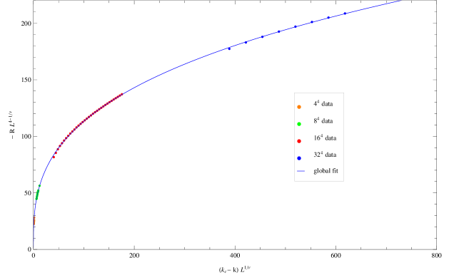
Figure 16: Finite size scaling behavior of the scaled curvature ${\cal R}(k,L)\cdot L^{4-1/\nu}$ versus the scaled coupling $(k_{c}-k)\cdot L^{1/\nu}$. Here $L=4,8,16,32$ for the lattice with $L^{4}$ sites. Statistical errors are comparable to the size of the dots. The continuous line represents a best fit to a scaling function of the form $a+b\,x^{c}$, and finite size scaling predicts that all points should lie on the same universal curve. The continuous line corresponds to a critical point $k_{c}=0.06388(32)$ and exponent $\nu=0.3334(4)$.

The finite size scaling properties of the curvature fluctuation, defined in Eqs. (15) and (16) will be discussed next. Again, if scaling involving $k$ and $L$ holds according to Eq. (88), with $t\sim k_{c}-k$ and $x_{O}=1-\delta=2-4\nu$ then all points should lie on the same universal curve. From the general form in Eq. (88) one expects for this particular case

$$\chi_{\cal R}(k,L)\;=\;L^{2/\nu-4}\;\left[\;\tilde{\chi_{\cal R}}\left((k_{c}-k)\;L^{1/\nu}\right)\;+\;{\cal O}(L^{-\omega})\;\right]\;\;\;\;,$$ (93)

where $\omega>0$ again a correction-to-scaling exponent. The above arguments then suggests that the quantity

$$\chi_{\cal R}(k,L)\cdot L^{4-2/\nu}\;\sim\;\left(L\over\xi\right)^{4-2/\nu}$$ (94)

should give points all lying on a single universal curve when displayed again as a function of the scaling variable $x$ in Eq. (91). Figure 17 shows a graph of the scaled curvature fluctuation $\chi_{\cal R}(k)/L^{2/\nu-4}$ for different values of $L=4,8,16,32$, versus the scaled variable $(k_{c}-k)L^{1/\nu}$. Using this method one finds approximately

$$k_{c}=0.06384(40)\;\;\;\;\;\nu=0.3389(56)\;\;\;\;.$$ (95)

Note that the errors in this case are much larger than for the corresponding average curvature analysis. Nevertheless the data supports such scaling behavior, and suggests again that $\nu$ is close to $1/3$.

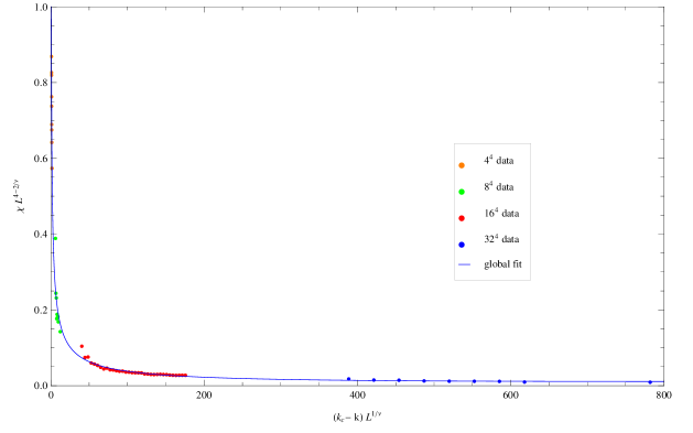
Figure 17: Finite size scaling behavior of the scaled curvature fluctuation $\chi_{\cal R}(k,L)\cdot L^{4-2/\nu}$ versus the scaled coupling $(k_{c}-k)\cdot L^{1/\nu}$. Here $L=4,8,16,32$ for a lattice with $L^{4}$ sites. The continuous line represents a best fit to a scaling function of the form $1/(a+b\,x^{c})$, and finite size scaling predicts that all points should lie on the same universal curve. The continuous line corresponds to a critical point $k_{c}=0.06384(40)$ and an exponent $\nu=0.3389(56)$.

The value of $k_{c}$ itself is expected to have a weak dependence on the linear size of the system $L_{0}\sim V^{1/d}$ . For a finite system of linear size $L_{0}$ one anticipates [52, 53] that close to the critical point

$$k_{c}(L_{0})\;\;\mathrel{\mathop{\sim}_{L_{0}\rightarrow\infty}}\;\;k_{c}(\infty)\,+\,c\;L_{0}^{-1/\nu}\;\;\;.$$ (96)

This is essentially the expression in Eq. (42), with $\xi\sim L_{0}$, and then solved for the finite volume critical point $k_{c}(L_{0})$. Indeed such a weak size dependence is found when comparing $k_{c}$ (as obtained from the algebraic singularity fits discussed previously) on different lattice sizes. Figure 18 shows the size dependence of the critical coupling $k_{c}$ as obtained on different size lattices. In all three cases $k_{c}(L_{0})$ is first obtained from a fit to the average curvature of the form ${\cal R}(k)\;=\;A\;(k_{c}-k)^{\delta}$ as in Eq. (44). Due to the few values of $L$ it is not possible at this point to extract an estimate for $\nu$ from this particular set of data. But since $\nu$ is close to $1/3$, it makes sense to use this value in Eq. (96), at least as a first approximation. So if one assumes $\nu=1/3$ exactly and extracts $k_{c}$ from a linear fit to $|{\cal R}|^{3}$, then the variations in $k_{c}$ for different size lattices are substantially reduced (points labeled by smalll circles in Figure 18). This then gives one additional independent estimate (which now combines all available lattice sizes, namely $L=4,8,16,32$)

$$k_{c}(\infty)\;\simeq\;0.063862\;\;$$ (97)

which is in good agreement with the value from the finite size analysis given in Eq. (92)

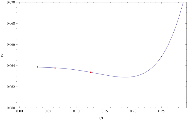
Figure 18: Size dependence of the critical point $k_{c}(L)$ for different lattices, with $N=L^{4}$ sites and $L=4,8,16,32$. The line represents a fit $k_{c}(L)=k_{c}(\infty)+A/L^{3}+B/L^{6}$ and gives the limiting estimate $k_{c}(\infty)=0.0638615$.

One physicsl quantity of significant interest is the fundamental gravitational correlation length $\xi(k)$ itself. It is defined via the exponential decay of physical correlations [such as the ones given in Eqs. (24) and (25)] as a function of the geodesic distance between points [see for example Eq. (27)]. It also appears as the quantity of key significance in the scaling argument for the free energy [see Eq. (41)], and is expected to diverge in accordance with Eq. (42) in the vicinity of the critical point at $k_{c}$. The discussion given in the previous sections pointed to the fact that this quantity is small and of the order of one average lattice spacing ($\xi\sim l_{0}$) in the strong coupling limit (small $k$), and is expected to increase monotonically towards the critical point at $k_{c}$ in accordance with Eq. (42). Indeed all the results presented in the previous two sections have been analyzed in terms of universal scaling properties in accordance with the basic assumption of Eq. (41), and all the results that follow from it. From the results presented so far one concludes that the correlation length exponent $\nu$ defined in Eq. (42) is consistent with $\nu=1/3$.

The next step is to fix the correlation length critical amplitude $A_{\xi}$ as well, which is defined in Eq. (42). The latter is not obtained in an obvious way from any of the results presented so far, and requires instead a direct and separate computation of physical correlations at fixed geodesic distance, such as the one in Eq. (27). These correlations were already computed in [25], and additional estimates on the correlation length $\xi$ and can be obtained separately from the size or volume dependence of local averages, which is expected to behave, for fixed $k\neq k_{c}$ but close to the critical point, as

$${\cal R}_{L_{0}}(k)\;\;\mathrel{\mathop{\sim}_{L_{0}\,\gg\,\xi}}\;\;{\cal R}_{\infty}(k)\,+\,{A\over\sqrt{\xi}\,L_{0}^{3/2}}\;e^{-L_{0}/\xi}$$ (98)

where here $L_{0}\sim V^{1/4}$ is a suitably defined linear size of the system. Nevertheless, the overall errors for this analysis can be reduced significantly if one assumes $\nu=1/3$ exactly (which from the previous results on ${\cal R}(k)$ and $\chi_{\cal R}(k)$ is known to be a very good approximation), and furthermore if one assumes that the correlation length diverges at one and the same critical $k_{c}$ (also determined to great accuracy from the previous results for ${\cal R}(k)$ and $\chi_{\cal R}(k)$). The latter set of results was largely based on the scaling assumption in Eq. (41). Given these simplifying choices one then obtains

$${\cal R}(k)\;\;\mathrel{\mathop{\sim}_{k\,\rightarrow\,k_{c}}}\;\;(k_{c}\,-\,k)^{d\,\nu-1}\;\sim\;\xi^{1/\nu-d}\;\sim\;1/\xi\;\;,$$ (99)

and also

$$\chi_{\cal R}(k)\;\;\mathrel{\mathop{\sim}_{k\,\rightarrow\,k_{c}}}\;\;(k_{c}\,-\,k)^{d\,\nu-2}\;\sim\;\xi^{d/\nu-4}\;\sim\;\xi^{2}\;\;.$$ (100)

Therefore the two combinations ${\cal R}(k)\cdot\xi(k)$ and $\chi_{\cal R}(k)/\xi^{2}(k)$ are expected to approach a constant as $k\rightarrow k_{c}$. Computing these combinations is so far the most accurate way of determining the dependence on $k$ of $\xi(k)$, and in particular for establishing a numerical value for the key amplitude $A_{\xi}$ in Eq. (42). Via this route one finds close to $k_{c}$ that ${\cal R}\cdot\xi=A_{\xi}\cdot A_{\cal R}\simeq 19.57$ and $\chi_{\cal R}/\xi^{2}=A_{\chi}/A_{\xi}^{2}\simeq 2.216$, which then gives for the correlation length amplitude in Eq. (42) the estimate $A_{\xi}\simeq 0.80(3)$. A plot of the correlation length $\xi(k)$ obtained in this way is shown in Figure 19. Note that a knowledge of the amplitude $A_{\xi}$ then gives immediately, by the renormalization group equations in Eqs. (59), (61) and (63), the running of $G$ in the vicinity of the nontrivial fixed point at $G_{c}$.

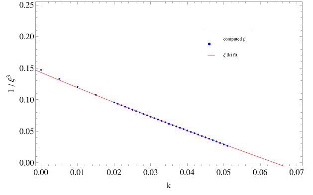
Figure 19: Estimate for the gravitational correlation length $\xi(k)$ versus bare coupling $k$. For a correlation length exponent $\nu=1/3$ [see Eq. (42)], $1/\xi(k)^{3}$ is expected to be linear in $k$ close to the critical point $k_{c}$.

10 Summary of Results

Table I summarizes the results obtained for the critical point $k_{c}=1/8\pi G_{c}$ and for the universal critical exponent $\nu$ obtained so far using a variety of observables and methods. In view of the detailed discussion of the previous section one finds from the best data so far (the one with the smallest statistical uncertainties, and the least systematic effects)

$$k_{c}=0.063862(18)\;\;\;\;\;\nu=0.334(4)\;\;\;\;,$$ (101)

which is consistent with the conjecture that $\nu=1/3$ exactly for pure quantum gravity in four dimensions. In turn this gives for the bare coupling $G$ at the critical point

$$G_{c}\;=\;{1\over 8\pi k_{c}}\;=\;0.623042(25)\;\;.$$ (102)

In previous work [48] the following estimates were given

$$k_{c}=0.0636(11)\;\;\;\;\;\nu=0.33(1)\;\;\;\;,$$ (103)

which have been refined in view of the higher statistics and larger lattices which are part of the current study.

Observables used to compute $k_{c}$ and $\nu$	Critical Point $k_{c}$	Universal Exponent $\nu$
Average Curvature ${\cal R}$ vs. $k$	0.06336(28)	0.331(4)
Average Curvature ${\cal R}^{3}$ vs. $k$	0.06367(29)	0.332(2)
Average Curvature ${\cal R}^{3}$ vs. $k$	0.06407(24)	-
Curvature Fluctuation $\chi_{\cal R}$ vs. $k$	0.05383(102)	0.350(56)
Curvature Fluctutation $\chi_{\cal R}$ vs. $k$	-	0.321(12)
Curvature Fluctuation $\chi_{\cal R}^{-3/2}$ vs. $k$	0.06369(84)	-
Logarithmic Derivative $2\langle l^{2}\rangle\chi_{\cal R}/{\cal R}$ vs. $k$	0.06338(56)	0.336(8)
Curvature Fluctuation $\chi_{\cal R}$ vs. ${\cal R}$	-	0.332(7)
${\cal R}(k,L)$ Finite Size Scaling	0.06388(11)	0.333(2)
$\chi_{\cal R}(k,L)$ Finite Size Scaling	0.06384(18)	0.339(6)
Size Dependence of the Critical Point $k_{c}(L)$	0.063862(30)	-

TABLE I. Summary of results for the critical point $k_{c}$ and the universal gravitational critical exponent $\nu$, as obtained from the largest lattices studies so far.

Table II provides a comparison between the best lattice estimate given in Eq. (101) and the value of the universal exponent $\nu$ from other approaches. These include the calculation of $\nu$ in the $2+\epsilon$ expansion for gravity [22] carried out to two loop order [23], a calculation of the same using a truncated renormalization group approach in four dimensions [55, 56], including some recent more refined estimates [57]. Further references include a simple geometric argument based on geometric features of the graviton vacuum polarization cloud, which gives $\nu=1/(d-1)$ for large $d$ [33], and the rough estimate for $\nu$ from the lowest nontrivial order strong coupling expansion for the gravitational Wilson loop [29], which gives $\nu=1/2$. Finally the result of [46] is mentioned, where it was found that a solution to the nonlocal effective field equations of Eq. (62) for the static isotropic metric can only be found provided $\nu=1/(d-1)$ exactly for $d\geq 4$. For a plot of the corresponding values for $\nu$ see Figure 20.

Method used to compute $\nu$ in d=4	Universal Exponent $\nu$
Euclidean Lattice Quantum Gravity (this work)	$\nu^{-1}=2.997(9)$
Perturbative $2+\epsilon$ expansion to one loop [22]	$\nu^{-1}=2$
Perturbative $2+\epsilon$ expansion to two loops [23]	$\nu^{-1}=22/5=4.40$
Einstein-Hilbert RG truncation [56]	$\nu^{-1}\approx 2.80$
Recent improved Einstein-Hilbert RG truncation [57]	$\nu^{-1}\approx 3.0$
Geometric argument [33] $\rho_{vac\;pol}(r)\sim r^{d-1}$	$\nu^{-1}=d-1=3$
Lowest order strong coupling (large G) expansion [29]	$\nu^{-1}=2$
Nonlocal field equations with $G(\Box)$ for the static metric [46]	$\nu^{-1}=d-1$ for $d\geq 4$

TABLE II. A comparison of estimates for the fundamental scaling exponent $\nu$, based on a variety of different analytical and numerical methods. These include the $2+\epsilon$ expansion for pure gravity carried out at one and two loops [22], an estimate for the leading exponent in a truncated renormalization group expansion [56, 57], a simple geometric argument based on the geometric features of the quantum vacuum polarization cloud for gravity, and finally the only value allowed by a consistent solution to the nonlocal field equation with a $G(\Box)$ for the static isotropic metric.

Table III then gives a similar table, where values for the universal gravitational critical exponent $\nu$ are given in three dimensions (for the Euclidean case) or $2+1$ dimensions (for the Lorentzian case). Here again it is possible to make a direct comparison between several approaches, namely the lattice [58, 47], the two-loop $2+\epsilon$ expansion of [23] but with now $\epsilon=1$, the Einstein-Hilbert truncated renormalization group approach [55, 56, 57] and the large $d$ estimate of [33]. The corresponding values for $\nu$ are shown in Figure 20.

Method used to compute $\nu$ in $d=3$	Universal Exponent $\nu$
Euclidean Lattice Quantum Gravity [58]	$\nu^{-1}=1.72(5)$
Exact solution of Lorentzian Gravity (Wheeler-DeWitt Eq.) in 2+1 dim. [47]	$\nu^{-1}=11/6=1.8333$
Perturbative $2+\epsilon$ expansion to one loop [22]	$\nu^{-1}=1$
Perturbative $2+\epsilon$ expansion to two loops [23]	$\nu^{-1}=8/5=1.6$
Einstein-Hilbert RG truncation [56]	$\nu^{-1}\approx 1.33$
Large $d$ geometric argument [33] $\rho_{vac\;pol}(r)\sim r^{d-1}$	$\nu^{-1}=d-1=2$

TABLE III. A comparison of various estimates for the fundamental scaling exponent $\nu$ in $2+1$ dimensions, based on a variety of different analytical and numerical methods. Included are the $2+\epsilon$ expansion for pure gravity carried out at one and two loops [22, 23], an estimate for the leading exponent in a truncated renormalization group expansion [56], and a simple geometric argument based on general features of the quantum vacuum polarization cloud for gravity.

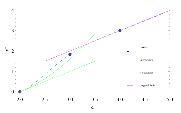
Figure 20: Universal scaling exponent $\nu$ determining the running of $G$ [see Eqs. (59) and (61)] as a function of spacetime dimension $d$. Shown are the results in $2+1$ dimensions obtained from the exact solution of the lattice Wheeler-DeWitt equation [47], the numerical result in four dimensions (this work and [48]), the $2+\epsilon$ expansion result to one [22] and two loops [23], and the large $d$ result $\nu^{-1}\simeq d-1$ [33]. For actual numerical values see Tables II and III.

11 Implications from a Gravitational Exponent $\nu=1/3$

In this section the consequences of having a definite value for the critical point $k_{c}$, as well as a value for the universal critical exponent $\nu$ [see Eq. (101], will be discussed. One notes on the one hand that the value for $k_{c}$ and thus $G_{c}$ now fixes the value for the ultraviolet cutoff $a$. At the same time, the specific value for $\nu\simeq 1/3$ gives predictions for the scaling behavior of local averages, gravitational correlations and the running of $G$.

First note that the value for the critical point $k_{c}$ given in Eqs. (101) and (102) fixes the lattice spacing $a$, and thus the value for the ultraviolet cutoff

$$G\;\approx\;G_{c}\;=0.623041\,a^{2}\;\;.$$ (104)

From the known laboratory value of Newton’s constant $G$, $l_{P}\equiv\sqrt{\hbar G/c^{3}}$$=1.616199(97)\times 10^{-33}cm$, so that one obtains for the fundamental lattice spacing $a=1.2669\,\sqrt{G_{c}}\,\equiv\,l_{P}$, or

$$a\;=\;2.0476\,\times\,10^{-33}\,cm\;\;.$$ (105)

and from it a definite value for the ultraviolet cutoff $\Lambda\simeq 1/a$. For the average lattice spacing in units of $a$ one finds

$$<\!l^{2}\!>\;\equiv\;l_{0}^{2}\;=[\,2.398(9)\,a\,]^{2}$$ (106)

so that $a$ and $l_{0}$ are quite comparable in magnitude [this fact can be traced back to the original overall scale choice $\lambda_{0}=1$ in Eqs. (2) and (6), motivated by Eq. (10)].

For the average local curvature ${\cal R}(k)$ one has from Eq.(44), using Eq.(42) and $\nu=1/3$,

$${<\int d^{4}x\,\sqrt{g}\,R(x)>\over<\int d^{4}x\,\sqrt{g}>}\;\sim\;\xi^{1/\nu-d}\;\sim\;{A^{\prime}_{\cal R}\over a\;\xi}\;\;.$$ (107)

The dimensionless amplitude $A^{\prime}_{\cal R}$ is expected to be $O(1)$ in lattice units, and is given below in Eq. (111). This result is based on the fact that the lattice calculations allow one to also extract various amplitude coefficients. For the dimensionless curvature amplitude defined in Eq. (44) one finds

$$A_{\cal R}\;=\;24.46(9)\;\;,$$ (108)

and for the dimensionless curvature fluctuation amplitide defined in Eq. (45)

$$A_{\chi}\;\equiv\;{4\,\nu-1\over<\!l^{2}\!>}\,A_{\cal R}\;=\;1.418(6)\;\;.$$ (109)

Combined with the dimensionless correlation length amplitude defined in Eq. (42)

$$A_{\xi}\;=\;0.80(3)\;\;$$ (110)

one finds for the amplitude in Eq. (107)

$$A^{\prime}_{\cal R}\;\equiv\;{A_{\cal R}\,A_{\xi}\over<\!l^{2}\!>}\;=\;3.40(13)\;\;.$$ (111)

For the curvature fluctuation $\chi_{\cal R}(k)$ one has from Eqs. (15), (45) and (100)

$${<(\int d^{4}x\,\sqrt{g}\,R)^{2}>-<\int d^{4}x\,\sqrt{g}\,R>^{2}\over<\int d^{4}x\,\sqrt{g}>}\;\sim\;\xi^{2/\nu-d}\;\sim\;A^{\prime}_{\chi}\,\xi^{2}/a^{2}\;\;.$$ (112)

with dimensionless amplitude

$$A^{\prime}_{\chi}\;\equiv\;{A_{\chi}\,\over A_{\xi}^{2}}\;=\;{4\,\nu-1\over<\!l^{2}\!>}\cdot{A_{\cal R}\over A_{\xi}^{2}}\;=\;2.22(9)\;\;.$$ (113)

These results in turn provide useful information for the curvature correlation function at fixed geodesic distance of Eqs. (24) and (25). From Eq.(48) one has for the power appearing in Eq. (26) $2n=2\,(d-1/\nu)=2(4-3)=2$

One then obtains for the curvature-curvature correlation function at “short distances” $r\ll\xi$ and for $\nu=1/3$ the remarkably simple result

$$<\sqrt{g}\;R(x)\;\sqrt{g}\;R(y)\;\delta(|x-y|-d)>_{c}\;\;\mathrel{\mathop{\sim}_{d\;\ll\;\xi}}\;\;{1\over d^{\,2\,d-2/\nu}}\;\sim\;{A_{0}\over a^{2}\,d^{2}}\;\;.$$ (114)

Note that in the last term the correct dimensions have been restored, by inserting suitable powers of the lattice spacing $a$. It is instructive to compare the above result to the expression for the local average curvature, Eq. (107); note in particular that both expressions still contain explicitly the size of the microscopic parallel transport loop $\sim a\sim l_{P}$. Here the dimensionless amplitude $A_{0}$ is related to the amplitude in Eq. (113) because of Eq. (47), and one finds

$$A_{0}\;\equiv\;{A^{\prime}_{\chi}\over 2\pi^{2}}\;=\;{1\over 2\pi^{2}}\cdot{1\over 3}\cdot{1\over<\!l^{2}\!>}\cdot{A_{\cal R}\over A_{\xi}^{2}}\;=\;[\,0.335(20)\,]^{2}$$ (115)

so that the dimensionless correlation function normalization constant is $N_{R}\,\equiv\,\sqrt{A_{0}}=0.335(20)$. As expected, all of these amplitudes are close to $O(1)$ in units of the ultraviolet cutoff (fundamental lattice spacing) $a$.

The exponent $\nu=1/3$ and the amplitude $A_{\xi}$ now determine the running of $G$ with scale, see Eq. (59), and one obtains

$$G(q^{2})\;=\;G_{c}\left[\;1\,+\,c_{0}\,\left({m^{2}\over q^{2}}\right)^{3/2}\,+\,O(\left({m^{2}\over q^{2}}\right)^{3})\;\right]\;\;,$$ (116)

with reference scale $m\equiv 1/\xi$. The coefficient $c_{0}$ [see Eq.(60)] determines the amplitude of the quantum correction, and it is given by

$$c_{0}\;=\;8\pi\,G_{c}\,A_{\xi}^{1/\nu}\;=\;A_{\xi}^{3}/k_{c}\;\;,$$ (117)

with $A_{\xi}=0.80(3)$ from the numerical solution [see Eq. (110); for the definition of the amplitude $A_{\xi}$ see Eq. (42)], and also $\nu=1/3$ and $k_{c}$ from Eq. (101). This then gives for the dimensionless amplitude of the leading quantum correction in Eq. (116) $c_{0}\approx 8.02$. This last result can then be translated directly into a covariant $G(\Box)$ [see Eq. (61) with $\nu=1/3$],

$$G(\Box)\;=\;G_{c}\left[\;1\,+\,c_{0}\,\left({1\over-\xi^{2}\,\Box^{2}}\right)^{3/2}\,+\,\dots\;\right]\;\;.$$ (118)

The latter forms the basis for a set of nonlocal effective field equations [see Eq. (62)], and gives the running of $G(r)$ for the specific choice of the static isotropic metric [see Eq. (63)].

In principle it is also possible to estimate the next (sub-leading) correction to the leading running of $G$ in Eq. (116), given the knowledge of the subleading corrections to $\xi(k)$ or $m(k)$ in Eqs. (42) or (116). If one has

$$\xi^{-1}(G)\;=\;a^{-1}\,A_{m}\,(G\,-\,G_{c})^{\nu}\,\left[1\,-\,b\,\nu^{2}\,(G\,-\,G_{c})\,+\,{\cal O}((G\,-\,G_{c})^{2})\right]\;\;,$$ (119)

with a sub-leading correction of amplitude $b$, then for the running of $G$ one obtains to this order

$${G(q^{2})\over G_{c}}\;=\;1\,+\,c_{0}\,\left({m^{2}\over q^{2}}\right)^{1/2\nu}\,+\,c_{1}\,\left({m^{2}\over q^{2}}\right)^{1/\nu}\,+\,\dots\,,$$ (120)

with $c_{1}=b\,\nu/(A_{m}^{2/\nu}\,G_{c})\approx 2.87$, given that $b\approx 0.215$ and $A_{m}=(k_{c}/G_{c})^{\nu}/A_{\xi}$, and $A_{\xi}$ given in Eq. (110). The domain of validity for the above expression is $q\gg m\equiv 1/\xi$ or $r\ll\xi$; the strong infrared divergence at $q\simeq 0$ is largely an artifact of the current expansion, and can be regulated either by cutting off the momentum integrations at $q\simeq m=1/\xi$, or by the replacement on the r.h.s. $q^{2}\rightarrow q^{2}+m^{2}$.

Furthermore, the previous results show clearly that the reference scale for the running of $G$ is set by the correlation length $\xi$, which by Eqs. (46), (99) and Eqs. (107) appears to be directly related to curvature. In particular the form of the running of $G$ with scale suggests that no detectable corrections to classical gravity should arise until either a) the scale $r$ approaches the very large (cosmological) scale $\xi$, or b) until one reaches extremely short distances comparable to the Planck length $r\sim l_{p}$, at which point higher derivative terms, light matter corrections and string contributions come into play. In other words, the results of Eqs. (63) (116) or (118) imply that classical gravity is largely recovered on atomic, laboratory, solar and even galactic scales, as long as the relevant distances satisfy $r\ll\xi$.

Therefore one crucial ingredient needed in pinning down the magnitude of the quantum correction for $G(q^{2})$ in Eqs. (116) or (118) is the actual value of the nonperturbative reference scale $\xi$. It was argued in [29] that, in analogy to ordinary gauge theories, the gravitational Wilson loop provides precisely such an insight. The main points of the argument are rather simple and can be reproduced in a few lines. In complete analogy to the gauge theory case, these arguments basically rely on the concept of universality, the existence of a universal correlation length at strong coupling, and the use of the Haar invariant measure to integrate over large fluctuations of the fundamental local parallel transport matrices. Following [26, 27], in [29] the vacuum expectation value corresponding to the gravitational Wilson loop was defined as

$$<W(C)>\;=\;<\mathop{\rm tr}\left[\,\omega(C)\;U_{1}\;U_{2}\;...\;U_{n}\right]>\;\;.$$ (121)

Here the $U$’s are elementary rotation matrices, whose form is determined by the affine connection and which therefore describe the parallel transport of vectors around a loop $C$, see also Eq. (32). Here $\omega_{\mu\nu}(C)$ is a constant unit bivector, characteristic of the overall geometric orientation of the loop, giving the normal to the loop. In the continuum the combined rotation matrix ${\bf U}(C)$ is given by the path-ordered (${\cal P}$) exponential of the integral of the affine connection $\Gamma^{\lambda}_{\mu\nu}$, as in Eq. (31), so that the previous expression represents a suitable regularized and discretized lattice form. In [29] it was then shown that quite generally in lattice gravity for sufficiently strong coupling one obtains universally an area law for near planar loops,

$$<W(C)>\;\simeq\;\exp\,(-\,A_{C}/{\xi}^{2})$$ (122)

where $A_{C}$ is the geometric area of the loop. This last result relies on a modified first order formalism for the Regge lattice theory [34], in which the lattice metric degrees of freedom are separated out into local Lorentz rotations and tetrads. Moreover, the result of Eq. (121) appears be universal since and was shown to hold in all known lattice formulations of quantum gravity in the strong coupling regime. In [29] an expression for the correlation length $\xi$ appearing in Eq. (122) was given in the strong coupling limit, where one finds $\xi=4/\sqrt{k_{c}\,|\log(k/k_{c})|\,+\,O(k^{2})}$. For $k$ close to $k_{c}$ this gives immediately $\xi\,\simeq\,4\,|k_{c}-k|^{-1/2}$ and thus, to this order, $\nu=\textstyle{1\over 2}\displaystyle$ and also $A_{\xi}=4$ in Eq. (42). Nevertheless, the discussion of the previous sections and the numerical solution of the full lattice theory suggests that the correct expression for $\xi$ to be used in Eq. (122) should be the one in Eq. (42), with $\nu=1/3$ [Eq. (101)], $k_{c}$ given in Eq. (101) and amplitude $A_{\xi}=0.80(3)$.

The next step is to make contact between the above results and a semiclassical description, which requires that one connects the nonperturbative result of Eq. (122) to a suitable semiclassical physical observable. Indeed, by the use of Stokes’s theorem, semiclassically the parallel transport of a vector round a very large loop depends on the exponential of a suitably coarse-grained Riemann tensor over the loop. In this semiclassical picture one has for the combined rotation matrix ${\bf U}$

$$U^{\mu}_{\;\;\nu}(C)\;\sim\;\Bigl{[}\;\exp\,\left\{\textstyle{1\over 2}\displaystyle\,\int_{S(C)}\,R^{\,\cdot}_{\;\;\cdot\,\lambda\sigma}\,A^{\lambda\sigma}_{C}\;\right\}\,\Bigr{]}^{\mu}_{\;\;\nu}\;\;,$$ (123)

where $A^{\lambda\sigma}_{C}$ is an area bivector associated with the loop in question,

$$A^{\lambda\sigma}_{C}=\textstyle{1\over 2}\displaystyle\oint_{C}dx^{\lambda}\,x^{\sigma}\;.$$ (124)

Then the semiclassical procedure gives for the loop in question

$$W(C)\,\simeq\,\mathop{\rm tr}\left(\,\omega(C)\,\exp\left\{\,\textstyle{1\over 2}\displaystyle\,\int_{S(C)}\,R^{\,\cdot}_{\;\;\cdot\,\lambda\sigma}\,A^{\lambda\sigma}_{C}\;\right\}\right)\;.$$ (125)

Here again $\omega_{\mu\nu}(C)$ is a constant unit bivector, characteristic of the overall geometric orientation of the parallel transport loop. By carefully comparing coefficients for the two area terms [29] one then concludes that the average large-scale curvature is of order $+1/{\xi}^{2}$, at least in the strong coupling limit considered in the cited references. Since the scaled cosmological constant can be viewed as a measure of the intrinsic curvature of the vacuum, the above argument then gives a positive cosmological constant for this phase, corresponding to a manifold which behaves as de Sitter ($\lambda>0$) on large scales [29]. These arguments then lead to the suggestion that the macroscopic (semiclassical) average curvature is related to $\xi$ by

$$\langle\,R\,\rangle_{\rm large\;scales}\;\;\sim\;+\,1/\xi^{2}\;\;,$$ (126)

at least in the strong coupling (large $G$) limit. It is important to note here that the result of Eq. (126) applies to parallel transport loops whose linear size $r_{C}$ is much larger than the cutoff, $r_{C}\gg l_{p},a$; neverthless in this limit the answer for the macroscopic curvature in Eq. (126) becomes independent of the loop size or its area [29]. Furthermore, these arguments lead, via the classical field equations, to the identification of $1/\xi^{2}$ with the observed (scaled) cosmological constant $\lambda_{obs}$,

$$\textstyle{1\over 3}\displaystyle\;\lambda_{obs}\;\simeq\;+\,{1\over\xi^{2}}\;.$$ (127)

In this picture the latter is then regarded as the quantum gravitational condensate, a measure of the vacuum energy, and thus of the intrinsic curvature of the vacuum. Then a suitable effective action, describing the residual effects of quantum gravity on very large distance scales, is of the form

$$I_{\rm eff}\,[g_{\mu\nu}]\;=\;-\,{1\over 16\pi\,G(\mu)}\int d^{4}x\,\sqrt{g}\;\Bigl{(}R\,-\,{6\over\xi^{2}}\Bigr{)}\,+\,I_{\rm matter}\,[g_{\mu\nu},\dots]\;\;,$$ (128)

with $G(\mu)$ a very slowly varying (on macroscopic scales) Newton’s constant, in accordance with Eqs. (116) or (118).

Note that the above results in many ways parallels what is found in non-Abelian gauge theories, where for example one has for the color condensate $<F_{\mu\nu}^{2}>\,\simeq 1/\xi^{4}$. Furthermore, this last result can also be obtained largely from purely dimensional grounds, once the existence of a fundamental correlation length $\xi$, which for QCD is given by the inverse of the mass of the lowest spin zero glueball, is established. Accordingly, for gravity too one would expect, again simply on the basis of dimensional arguments, that the large scale curvature (the graviton condensate) should be related to the fundamental correlation length by $\langle\,R\,\rangle\,\simeq\,1/\xi^{2}$, as in Eq. (46).

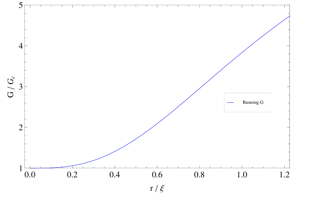
Figure 21: Running gravitational coupling $G(r)$ versus $r$, obtained from the $G(k)$ in Eq. (59) by setting $q\sim 1/r$, with exponent $\nu=1/3$ and amplitude $a_{0}\simeq 8.02(55)$. The lattice quantum gravity calculations done so far suggest roughly a 5% effect on scales of $0.187\times 4890Mpc\approx 910Mpc$, and a 10 % effect on scales of $0.238\times 4890Mpc\approx 1160Mpc$.

The considerations presented so far can to some extent finally provide a quantitative handle on the physical magnitude of the nonperturbative scale $\xi$. From the observed value of the cosmological constant one obtains an estimate for the absolute magnitude of the scale $\xi$

$$\xi\;\simeq\;\sqrt{3/\lambda}\;\approx\;4890Mpc\;\;.$$ (129)

Irrespective of the specific value of $\xi$, this would indicate that generally the recovery of classical GR results only happens for distance scales much smaller than the correlation length $\xi$. In particular, the Newtonian potential acquires a tiny quantum correction from the running of $G(r)$,

$$V(r)\;=\;-\,G(r)\cdot{m_{1}\,m_{2}\over r}\;\;,$$ (130)

with $G(r)$ given, for the static isotropic solution, in Eq. (63), and for which quantum effects become quite negligible on distance scales $r\ll\xi$. Figure 21 shows the expected qualitative behavior for the running $G(k)$ over scales slightly smaller or comparable to $\xi$, with the main uncertainty arising from estimating the physical magnitude of $\xi$ itself [Eq. (129)]. Specifically, from Eq. (59) the lattice prediction at this point is for roughly a 5% effect on scales of $0.184\times 4890Mpc\approx 900Mpc$, and a 10 % effect on scales of $0.232\times 4890Mpc\approx 1130Mpc$.

The above results also suggest that the curvature on very small scales behaves rather differently from the curvature on very large scales, due to the quantum fluctuations eventually averaging out. Indeed when comparing the result of Eqs. (46) and (99) to the one in Eq. (126) one is lead to conclude that the following change has to take place when going from small (linear size $\sim l_{p}$) to large (linear size $\gg l_{p}$) parallel transport loops

$$\langle\,R\,\rangle_{\rm small\;scales}\;\;\sim\;{1\over l_{p}\,\xi}\;\;\;\;\;\rightarrow\;\;\;\;\;\langle\,R\,\rangle_{\rm large\;scales}\;\;\sim\;{1\over\xi^{2}}\;.$$ (131)

An intuitive way of understanding the above result is that on small scales the strong local fluctuations in the metric/geometry lead to large values for the average rotation of a parallel-transported vector. But then on larger scales these short distance fluctuations tend to average out, and the combined overall rotation is much smaller, by a factor ${\cal O}(l_{p}/\xi)$,

$$Z_{R}\;=\;{l_{P}\over\xi}\;\;.$$ (132)

The above quantity should then be regarded as an essential and necessary “renormalization constant” when comparing curvature on different length scales, and specifically when going from very small (size $\sim l_{P}$) to large (size $\gg l_{P}$) parallel transport loops. See also the earlier discussion preceding Eq. (38), about the issue of comparing correlations of large loops versus correlations of small (infinitesimal) loops.

To conclude this section, one can raise the legitimate concern of how these results are changed by quantum fluctuations of various matter fields; so far all the results presented here apply to pure gravity without any matter fields. Therefore here and in the rest of the paper what has been followed is the quenched approximation, wherein gravitational loop effects (perturbative and nonperturbative) are fully accounted for, but matter loop corrections are entirely neglected. In the presence of matter fields coupled to gravity (scalars, fermions, vector bosons, spin-3/2 fields etc.) one would expect, for example, the value for $\nu$ to change due to vacuum polarization loops containing these fields. A number of arguments can be given though for why these effects should not be too dramatic, unless the number of light matter fields is rather large. Firstly one notices that to leading order in the $2+\epsilon$ expansion the exponent $\nu$ only depends on the dimensionality of spacetime, irrespective of the number of matter fields and of their type [22], $\nu\sim 1/(d-2)$. Also, one can show that in the $2+\epsilon$ expansion for gravity [22, 23] matter loop corrections appear later in the form of factors $\propto(25-c)$ in the $\beta$-function, where $c$ is the central charge corresponding to those massless matter fields. In four dimensions the correction is thought to be even smaller $\propto(48-c)$ [61]. Thus unless $c$ is rather large, the matter contribution is quite small even at next-to-leading order in the $2+\epsilon$ expansion [22, 23]. In addition, in the case of lattice gravity the effects of a single light scalar field are so small that they are barely detectable in the numerical evaluations of the path integral. In general one would expect significant infrared modifications to gravity coming from particles that are either massless or very nearly massless. The evidence so far would therefore suggests that the approximation in which vacuum polarization effects of light matter fields are entirely neglected should still be useful, at least as a first step.

12 Gravitational Scaling Dimensions and Phenomenology

The previous section dealt with the fact that one of the main implications of quantum gravity is the running of the gravitational constant with scale, in accordance with Eq. (61). There are additional consequences which arise from the fact that in general gravitational correlations don’t follow free field (gaussian) predictions. One example is the curvature correlation function of Eqs. (24), (26) and (48), for which the final form at this stage is given in Eq. (114). This section deals therefore with a discussion of the implications of the result given in this last expression for the curvature correlation function of Eq. (114), specifically with lattice spacing $a$ from Eq. (105) and amplitude given in Eq. (115), $N_{\cal R}\approx 0.335$.

There is clearly a rather substantial difference in scale between the curvature appearing in Eq. (24) and therefore in Eq. (114), and the curvature in Eq. (134). In the first case the curvature involves the parallel transport of vectors around infinitesimal loops, whose size is determined by the ultraviolet cutoff [the lattice spacing, comparable to the Planck length because of $G\approx G_{c}$ due to the slow running of $G$, with $G_{c}$ given in Eq. (102)]. In the second case the curvature in question refers instead to the semiclassical domain, as described by a set of effective long distance field equations, for which the curvature is obtained operationally from the parallel transport of vectors around macroscopic loops, of linear size much larger than the Planck length. Such a concern should be kept in mind when transitioning from the microscopic result in Eq. (114) to the semiclassical result written down below in Eq. (143).

First consider what can be stated purely at the classical level. One can use the field equations to directly relate the local curvature to the local matter mass density. From Einstein’s field equations

$$R_{\mu\nu}-\textstyle{1\over 2}\displaystyle\,g_{\mu\nu}\,R\;=\;8\pi G\,T_{\mu\nu}\;\;$$ (133)

for a perfect fluid one then obtains for the Ricci scalar, in the limit of negligible pressure,

$$R(x)\;\simeq\;8\pi G\;\rho(x)\;\;.$$ (134)

This last result then allows one to relate local fluctuations in the curvature $\delta\,R(x)$ to local fluctuations in the matter density $\delta\,\rho(x)$, which could potentially provide a useful connection to the quantum result for the correlation function in Eq. (26). Of course, in the Newtonian limit the above result simplifies to Poisson’s equation

$$\Delta\,h_{00}({\bf x},t)\;=\;8\pi\,G\,\rho({\bf x},t)\;\;,$$ (135)

where $h_{00}=2\phi$ and $\rho$ are the macroscopic gravitational field and the macroscopic mass density, respectively.

In the cosmology literature it is customary to describe matter density fluctuations in terms of the density contrast correlation function

$$G(r)\;=\;<\delta\rho(r)\;\delta\rho(0)>\;\;.$$ (136)

The latter is related to its Fourier transform $P(q)$ by

$$G(r)\;=\;{1\over 2\pi^{2}}\int_{\mu}^{\Lambda}dq\,q^{2}\,P(q)\,{\sin qr\over qr}\;,$$ (137)

and the above expression has to contain both an infrared regulator ($\mu$) and an ultraviolet cutoff ($\Lambda$), to make sure the integral converges. If the power spectrum $P(q)$ is described by a simple power law of the form

$$P(q)\;=\;{a_{0}\over q^{s}}\;\;,$$ (138)

(where $n=-s$ is commonly referred to as the spectral index), then one finds in the scaling regime $1/\mu\gg r\gg 1/\Lambda$ for the density contrast correlation function in real space

$$G(r)\;=\;c_{s}\,a_{0}\,\mu\,\Lambda^{2-s}\,\left({1\over\mu\,r}\right)^{3-s}\;\;,$$ (139)

with $c_{s}\equiv\Gamma(2-s)\,\sin(\pi s/2)\,/\,2\pi^{2}$. Not unexpectedly, the answer appears to be quite sensitive to the choice for the ultraviolet and infrared cutoffs. For the specific value $s=1$ one has $P(q)=a_{0}/q$, and this then gives

$$G(r)\;=\;\;{a_{0}\,\Lambda\over 2\pi^{2}\,\mu}\cdot{1\over r^{2}}\;\;\;\;\;\;(s=1)\;\;,$$ (140)

which would seem to reproduce the result in Eq. (114). In practice the observational data for such matter density correlations is often presented in the simple form [62]

$$G(r)\;=\;\left({r_{0}\over r}\right)^{\gamma}\;,$$ (141)

with exponent $\gamma$ and scale $r_{0}$ fitted to astrophysical observations. For an exponent $\gamma$ close to two, one has by comparing Eq. (140) to Eq. (141) $a_{0}\,=\,2\pi^{2}\,\mu\,r_{0}^{2}/\Lambda$, which still requires a choice of cutoffs $\mu$ and $\Lambda$; for the most obvious choice here, namely $\mu\simeq 1/\xi$ and $\Lambda\simeq 1/l_{P}$, one obtains

$$a_{0}\;=\;{2\pi^{2}\,l_{P}\over\xi}\cdot r_{0}^{2}\;\;.$$ (142)

It is rather tempting at this stage to try to connect the observational result of Eq. (141) to the quantum correlation function in Eq. (114). One then expects for the matter density fluctuation correlation also a power law decay of the form

$$<\delta\rho({\bf x},t)\;\delta\rho({\bf y},t^{\prime})>\;\;\;\mathrel{\mathop{\sim}_{|{\bf x}-{\bf y}|\;\ll\;\xi}}\;\;{1\over a^{2}(t)}\cdot{1\over a^{2}(t^{\prime})}\cdot{1\over|{\bf x}-{\bf y}|^{2}}\;\;$$ (143)

where $a(t)$ here represents the scale factor. Also, this last correlation function can be made dimensionless by suitably dividing it by the square of some average matter density $\rho_{0}\approx\rho_{c}=3H_{0}^{2}/8\pi G$. By comparing coefficients in Eqs. (114) and (141) one finds $\gamma=2$, and for the length scale in Eq. (141)

$$r_{0}\;=\;{1\over 8\pi\,G\,\rho_{0}}\cdot{\sqrt{A_{0}}\over a}\;,$$ (144)

with $\sqrt{A_{0}}\simeq 0.335$ the dimensionless amplitude for the curvature correlation function of Eq. (114), and $a$ the lattice spacing given in Eq. (105).

The preceding argument nevertheless still contains a fundamental flaw, related to the use, at this stage in unmodified form, of the curvature correlation function result of Eq. (114). As already discussed previously, that form applies to the correlation of infinitesimal (Planck length or cutoff size) loops, which would not seem to be appropriate for the macroscopic (or semiclassical) parallel transport loops, such as the ones that enter the field equations Eqs. (133) and (134), and which thus relate locally the macroscopic $\delta R(x)$ to the $\delta\rho(x)$. It would then seem desirable to be able to correct for the fact that the parallel transport loops sampled in Eq. (134) are much larger than the infinitesimal ones sampled in the correlation function in Eq. (114). As in Eqs. (38), (131) and (132), the transition to macroscopic loops (linear size $\gg a$) can be affected in Eq. (114) by the replacement of $a^{2}\rightarrow\xi^{2}$. This then gives for large (macroscopic size $\gg a$) parallel transport loops

$$<\sqrt{g}\;R(x)\;\sqrt{g}\;R(y)\;\delta(|x-y|-d)>_{c}\;\;\mathrel{\mathop{\sim}_{d\;\ll\;\xi}}\;\;{A_{1}\over\xi^{2}\,d^{2}}\;\;\;,$$ (145)

with the expectation of a comparable amplitude $A_{1}\approx A_{0}$. This last result then leads to the following improved estimate for the macroscopic matter density correlation of Eq. (136)

$$G(r)\;=\;\left({1\over 8\pi\,G}\right)^{2}\;{1\over\rho_{0}^{2}}\cdot{A_{1}\over\xi^{2}\;r^{2}}\;,$$ (146)

so that comparing to Eq. (141) one finds for the exponent $\gamma=2$, and for the length scale $r_{0}$ the improved value

$$r_{0}\;=\;{1\over 8\pi\,G\,\rho_{0}}\cdot{\sqrt{A_{1}}\over\xi}\;\approx\;0.380\;\xi\;$$ (147)

which seems more in line with observational data. For the Fourier amplitude $a_{0}$ in Eq. (138) one has now

$$a_{0}\;=\;2\pi^{2}\cdot{l_{P}\over\xi}\cdot r_{0}^{2}\;\approx\;2.85\;l_{P}\,\xi\;.$$ (148)

Observed galaxy density correlations give indeed for the exponent in Eq. (141) a value close to two, namely $\gamma\approx 1.8\pm 0.3$ for distances in the $0.1Mpc$ to $50Mpc$ range [62, 63], and for the length scale $r_{0}\approx 10Mpc$. More recent estimates for the exponent $\gamma$, going up to distance scales of $100Mpc$, range between $1.79$ and $1.84$ [64, 65, 66, 67, 68, 69]. Nevertheless at this point the (perhaps rather naive) identification given in Eqs. (147) and (148), while intriguing, is possibly entirely accidental since it bypasses any concerns about the actual physical origin of the galaxy correlation function in Eq. (144), including the form and evolution of primordial density perturbation, the detailed nature of linear relativistic density perturbation theory for a given comoving background etc.

13 Conclusions

In this work a number of improved estimates have been presented for gravitational scaling dimensions and amplitudes, obtained from the lattice theory of gravity. Numerical methods combined with modern renormalization group arguments and finite size scaling have been shown to provide detailed information about rather subtle nonperturbative aspects of the theory. It has been known for some time that the Euclidean lattice gravity theory has two phases, only one of which, the gravitational anti-screening phase for $G>G_{c}$, is physically acceptable. Here we have described in some detail the properties of the latter smooth phase, and provided quantitative estimates for the critical point, scaling dimensions and the behavior of physical correlations for distances large compared to the lattice cutoff. In many ways the present calculation is still incomplete, in particular the gravitational Wilson loop and the correlation between loops has not been studied numerically, and only some general properties have been inferred. Also, more heavy work is needed to accurately determine the curvature correlation functions versus distance, and from it the fundamental non-perturbative correlation length and various amplitudes connected to it. Furthermore, the derivation of a number of results has relied heavily on basic renormalization group scaling, with only a handful of explicit checks. Nevertheless, it would seem from the results presented so far that the feasibility of these types of calculations should increase significantly in the near term due to expected rapid advances in hardware and software tools.

It is encouraging that four different approaches to quantum gravity give rather comparable results for the scaling dimensions (see the comparison Tables II and III, as well as Figure 20), and therefore suggest a unique underlying renormalization group universality class, associated with the quantum version of General Relativity. It is characteristic of the model described here that the growth of $G$ with scale is described by a nonperturbative correlation length $\xi$, related to the gravitational vacuum condensate, for which a specific quantitative estimate was given earlier. More generally, the vacuum condensate picture of quantum gravity presented in this paper makes in principle a number of specific and testable predictions, which could either be verified or disproven in the near future, as new and increasingly accurate satellite observations become available. The main aspects of this picture can be summarized as follows:

1. The vacuum condensate picture of quantum gravity contains from the start a very limited number of parameters, and is therefore rather strongly constrained. While it does involve a new nonperturbative scale (the gravitational vacuum condensate), it is found that this scale simultaneously determines the running of $G$ with scale, the value of the scaled cosmological constant, and the long distance behavior of physical invariant correlations.

2. The current theory predicts a slow increase in strength of the gravitational coupling when very large, cosmological scales are approached [see Eqs. (116) and (118)]. In this context, the observed scaled cosmological constant $\lambda$ acts as a dynamically induced infrared cutoff, similar to what happens in non-Abelian gauge theories. In principle, both the universal power and amplitude for this infrared growth are calculable with some accuracy from the underlying lattice cutoff theory.

3. For a sufficiently large scale $\xi$ (and therefore small $\lambda$) no observable deviations from classical General Relativity are expected on laboratory, solar systems and even galactic scales [see Eqs. (63) and (130)].

4. The calculations presented here give a number of predictions for the behavior of invariant curvature correlations as a function of geodesic distance, and specifically the powers and amplitudes involved [see Eqs. (114) and (145)].

5. The lattice theory appears to exclude at this point the possibility of a physically acceptable phase with gravitational screening; such a (weak coupling) phase in the lattice theory appears to be inherently unstable, presumably as a consequence of the conformal mode, and cannot lead to a semiclassical regime for gravity. It leads instead to a pathological degenerate ground state describing some sort of branched polymer. Nevertheless for large enough quantum fluctuations (large $G$) the instability is overcome and a new stable phase emerges.

6. In the strong coupling limit (for the Euclidean case) of the lattice theory the effective, long distance cosmological constant is positive [29]. In this same regime it seems nearly impossible from the lattice theory to get a negative value for this quantity, irrespective of the choice of boundary conditions (which in the lattice context play no role in the argument). Also, a positive cosmological constant is interpreted here as a genuinely nonperturbative gravitational vacuum condensate [see Eqs. (126) and (127)].

If the picture presented in this paper is indeed close to correct, then it points to what appears to be a deep analogy between the nonperturbative vacuum state of quantum gravity and known properties of strongly coupled non-Abelian gauge theories (or what could be called the QCD analogy). Over time this analogy has been helpful in illustrating properties of quantum gravity, many of which are ultimately based on rather basic principles of the renormalization group, connected with the scaling properties expected in the vicinity of a nontrivial fixed point. Indeed in QCD there exists also a nonperturbative mass parameter $m=1/\xi$ (sometimes referred to as the mass gap) which is known to be a renormalization group invariant; that such a mass scale can be generated dynamically is known to be a highly nontrivial outcome of the renormalization group equations for QCD. Furthermore, there seems to be a fundamental relationship between the nonperturbative scale $\xi$ (or inverse renormalized mass) and a nonvanishing vacuum condensate for these theories, both for gravity and QCD,

$$\langle\,R\,\rangle\;\simeq\;{1\over\xi^{2}}\;\;\;\;\;\;\;\;\;\;\;\;\langle\,F_{\mu\nu}^{2}\,\rangle\;\simeq\;{1\over\xi^{4}}\;.$$ (149)

An additional relevant example that comes to mind is the fermion condensate in gauge theories,

$$\langle\,\bar{\psi}\psi\,\rangle\,\simeq\,{1\over\xi^{3}}\;,$$ (150)

a consequence of confinement and chiral symmetry breaking. Current lattice and phenomenological estimates for QCD cluster around $\langle\,{\alpha_{S}\over\pi}\,F_{\mu\nu}^{2}\,\rangle\;\simeq\;(440\,MeV)^{4}$ and $\langle\,\bar{\psi}\psi\,\rangle\,\simeq\,(290\,MeV)^{3}$ [70, 71, 72].

Modifications to the static potential in gauge theories are best expressed in terms of the running coupling constant $\alpha_{S}(\mu)$, whose scale dependence is determined by the celebrated beta function of $QCD$ with coupling $\alpha_{S}\equiv g^{2}/4\pi$. On the one hand, a solution of the renormalization group equations give for the running of $\alpha_{S}(\mu)$

$$\alpha_{S}(\mu)\;=\;{4\,\pi\over\beta_{0}\ln{\mu^{2}/\Lambda_{\overline{MS}}^{2}}}\,+\,\dots\;.$$ (151)

On the other hand, the nonperturbative scale $\Lambda_{\overline{MS}}$ appears as an integration constant of the renormalization group equations, and is therefore - by construction - scale independent,

$$\Lambda_{\overline{MS}}\;=\;\Lambda\,\exp\left({-\int^{\alpha_{S}(\Lambda)}\,{d\alpha_{S}^{\prime}\over 2\,\beta(\alpha_{S}^{\prime})}}\right)\;,$$ (152)

where here $\Lambda$ represents the QCD ultraviolet cutoff. The physical value of $\Lambda_{\overline{MS}}$ cannnot be fixed from perturbation theory alone and has to be determined instead from experiment, $\Lambda_{\overline{MS}}\simeq 210MeV$. In quantum gravity the corresponding statements are given in Eqs. (51) and (59).

Wilson loop correlations play an important role in QCD as they do in quantum gravity. In non-Abelian gauge theories a confining potential is found at strong coupling by examining the behavior of the Wilson loop, defined for a large closed loop $C$ as

$$\langle\,W(C)\,\rangle\,=\,\langle\,\mathop{\rm tr}{\cal P}\,\exp\Bigl{\{}ig\oint_{C}A_{\mu}(x)dx^{\mu}\Bigr{\}}\,\rangle\;\;,$$ (153)

with $A_{\mu}\equiv t_{a}A_{\mu}^{a}$ and the $t_{a}$’s the group generators of $SU(N)$ in the fundamental representation. In the pure gauge theory at strong coupling, the leading contribution to the Wilson loop is known to follow an area law for sufficiently large loops. The analogous quantity for gravity is the gravitational Wilson loop described, for example, in Eqs. (31) and (121). But in contrast to QCD, in gravity the Wilson loop bears no relationship to the static potential [30] (the path ordered line integral of the affine connection does not in any way describe a gravitational interaction energy).

A central role in this view of quantum gravity is played by the gravitational correlation length of Eqs. (27), (42) and (52). Gauge theories also contain a nonperturbative, dynamically generated quantity $\xi$, the gauge field correlation length, and it is essentially the same [up to a factor $O(1)$] as the inverse of $\Lambda_{\overline{MS}}$. The same universal quantity $\xi$ also appears in a number of other physical observables, including the exponential decay of the Euclidean correlation function for two infinitesimal loop operators separated by a distance $|x|$,

$$G_{\rm loop-loop}(x)\,=\,\langle\,\mathop{\rm tr}{\cal P}\exp\Bigl{\{}ig\oint_{C_{\epsilon}}A_{\mu}(x^{\prime})dx^{\prime\mu}\Bigr{\}}(x)\,\mathop{\rm tr}{\cal P}\exp\Bigl{\{}ig\oint_{C_{\epsilon}}A_{\mu}(x^{\prime\prime})dx^{\prime\prime\mu}\Bigr{\}}(0)\,\rangle_{c}\;\;.$$ (154)

Here the $C_{\epsilon}$’s are two infinitesimal loops centered around $x$ ands $0$ respectively, suitably defined on the lattice as, for example, elementary square loops. The gravitational analogue of such an (infinitesimal loop) correlation was given earlier in Eqs. (24) and (25). It is also understood that in gauge theories the inverse of the correlation length $\xi$ corresponds to the lowest mass excitation in the gauge theory, the scalar glueball with mass $m_{0}=1/\xi$. If the lightest scalar $0^{++}$ glueball has a mass of approximately $m=1750MeV$ (which then fixes $\xi=1/m$), then $\Lambda_{\overline{MS}}$ in QCD is about eight times smaller, which gives rise to what has been described in QCD as “precocious” scaling. So while the two scales are quite close, they do not necessarily coincide. And the same could be true in gravity.

Another important difference between gravity and QCD is that fact that in the former the ultraviolet cutoff still appears explicitly, hidden in the physical value of Newton’s constant $G$. There exists then a second scale $\xi$ whose magnitude is not directly related to the value of $G$; instead it reflects how close the bare $G$ is to the ultraviolet fixed point at $G_{c}$, and is therefore fine tuned in this approach (just like a mass squared term in a scalar field theory). In QCD on the other hand the scale $\xi$ appears explicitly, wheras the ultraviolet cutoff is deeply hidden in the renormalization group relationship between $\Lambda_{\overline{MS}}$ and the bare coupling at the cutoff scale $\alpha_{S}(\Lambda)$.

Acknowledgements

The work of the author was supported in part by the Max Planck Gesellschaft zur Förderung der Wissenschaften, and by the University of California. He wishes to thank prof. Hermann Nicolai and the Max Planck Institut für Gravitationsphysik (Albert-Einstein-Institut) in Potsdam for warm hospitality. The author is also grateful for useful discussions with James Hartle and Gabriele Veneziano. The numerical calculations described in this paper were performed in part on the supercomputers located at the $AEI$.

Appendix

Appendix A Details on the parallel code

A few details will be given here regarding the performance of the computer code used on the Datura Supercomputer at AEI. The latter is a high performance Infiniband cluster, primarily used for large scale numerical calculations in classical General Relativity. The cluster is based on Intel Xeon X5650 2.66 GHz processor boards which have two processors per board, each with six cores. Thus there are 12 cores per board, 200 nodes and 2400 cores total. The main communication and storage network is based on an Infiniband QDR 324-port 40Gbit/s low latency and high bandwidth switch. In addition, the Datura cluster is equipped with 4,800 GB of main memory, corresponding to 2GB per core.

There are presently two main versions of the lattice quantum gravity code, a scalar (sequential) one and a parallel code. Both codes run exclusively in double precision (64 bits). The scalar code takes about 1021 seconds per iteration on a lattice with $32^{4}=1,048,576$ sites, which includes updates with an action containing higher derivative terms. The scalar code performance on a single core is measured (by counting raw floating point operations using a hardware performance monitor) at 3.3 GFlops.

In the case of the parallel code, on a $16^{4}$ lattice (1,572,864 simplices) the edges emanating from 256 sites can all be updated in parallel, with the work distributed on 256 cores. A whole lattice is therefore updated in 256 passes, and it takes about 0.26 seconds per iteration for a whole lattice.

On the $32^{4}$ lattice (25,165,824 simplices) the edges emanating from 256 sites are all updated in parallel, with the work distributed again on 256 cores. A whole lattice is therefore updated here in 4096 passes, and it takes about 4.01 seconds per iteration for a whole lattice. Thus for this setup the parallel codes is about 255 times faster than the single core scalar code. The MPI communication overhead between nodes for this setup accounts for only about 1%. Using 256 cores the overall code performance on this machine is around 845 GFlops.

On the $64^{4}$ lattice (402,653,184 simplices) the edges emanating from 256 sites are all updated in parallel, with the work distributed on 256 cores. A whole lattice is therefore updated now in 65,536 passes. This then gives about 64 seconds per iteration. When a full complement of 1024 cores are used instead of 256, the time for one full lattice iteration goes down to about 16 seconds. With a full 1024 cores used in parallel the overall code performance on this machine is around 3.4 TFlops. If even more cores are used, the code performance should further improve provided the network bandwidth is commensurate.

References

- [1] K. G. Wilson, Feynman-graph expansion for critical exponents, Phys. Rev. Lett., 28, 548 (1972); Quantum field-theory models in less than 4 dimensions, Phys. Rev. D, 7, 2911 (1973).
- [2] K. G. Wilson, The Renormalization Group: Critical Phenomena and the Kondo Problem, Rev. Mod. Phys., 47, 773 (1975); The Renormalization Group and Critical Phenomena, Rev. Mod. Phys., 55, 583 (1983).
- [3] G. Parisi, On the renormalizability of not renormalizable theories, Lett. Nuovo Cim. 6S2, 450 (1973); Theory of Non-Renormalizable Interactions - The large N expansion, Nucl. Phys. B100 368 (1975).
- [4] G. Parisi, On Non-Renormalizable Interactions, in the proceedings of the 1976 Cargése NATO Advances Study Institute, on New Developments in Quantum Field Theory and Statistical Mechanics (M. Levy and P. Mitter eds., Plenum Press 1977).
- [5] T. Regge, General Relativity without Coordinates, Nuovo Cimento, 19 558 (1961).
- [6] J. A. Wheeler, Geometrodynamics and the Issue of the Final State, in Relativity, Groups and Topology, 1963 Les Houches Lectures, eds. B. DeWitt and C. DeWitt (New York, Gordon and Breach, 1964).
- [7] H. W. Hamber, Quantum Gravitation - The Feynman Path Integral Approach, Springer Tracts in Modern Physics (Springer, New York, 2009).
- [8] R. P. Feynman, Quantum Theory of Gravitation, Acta Phys. Pol. 24 (1963) 697; Lectures on Gravitation, 1962-1963, edited by F. B. Morinigo and W. G. Wagner, California Institute of Technology (Pasadena, 1971).
- [9] B. DeWitt, Quantum Theory of Gravity,Phys. Rev. 160 1113 (1967); Phys. Rev. 162 1195 and 1239 (1967).
-
[10]
E.S. Fradkin and A.A. Tseytlin, Phys. Lett. 104B (1981) 377
and 106B (1981) 63;
Nucl. Phys. B201 (1982) 469;
I.G. Avramidy and A.O. Barvinsky, Phys. Lett. 159B (1985) 269. - [11] S. W. Hawking, in ‘General Relativity - An Einstein Centenary Survey’, edited by S. W. Hawking and W. Israel, (Cambridge University Press, 1979).
-
[12]
G. W. Gibbons and S. W. Hawking,
Phys. Rev. D 15, 2752 (1977) ;
S. W. Hawking, Phys. Rev. D 18, 1747 (1978);
G. W. Gibbons, S. W. Hawking and M. J. Perry, Nucl. Phys. B 138, 141 (1978). - [13] R. P. Feynman and A. Hibbs Quantum Mechanics and Path Integrals, (McGraw-Hill, New York, 1965).
- [14] H. W. Hamber, Simplicial Quantum Gravity, in Critical Phenomena, Random Systems and Gauge Theories, 1984 Les Houches Summer School, Session XLIII, (North Holland, Amsterdam, 1986).
- [15] G. Parisi, Statistical Field Theory; Benjamin Cummings (San Francisco, CA, USA, 1981).
- [16] J. Zinn-Justin, Quantum Field Theory and Critical Phenomena, 4th ed.; Oxford University Press (Oxford, UK, 2002).
- [17] J. Cheeger, W. Müller and R. Schrader, in Heisenberg Symposium, München, Germany, 1981, Springer Lecture Notes in Physics, edited by P. Breitlohner and H. P. Dürr (Springer, New York, 1982); Comm. Math. Phys. 92, 405 (1984).
- [18] M. Roc̆ek and R. M. Williams, Phys. Lett. 104B, 31 (1981); Z. Phys. C21, 371 (1984).
- [19] H. W. Hamber and R. M. Williams, Nucl. Phys. B 248, 392 (1984); 260, 747 (1985); 269, 712 (1986); Phys. Lett. B 157, 368 (1985).
-
[20]
R. Gastmans, R. Kallosh and C. Truffin, Nucl. Phys. B133
(1978) 417;
S. M. Christensen and M. J. Duff, Phys. Lett. B79 (1978) 213. - [21] S. Weinberg, Ultraviolet Divergences in Quantum Gravity, in ’General Relativity - An Einstein Centenary Survey’, edited by S. W. Hawking and W. Israel, (Cambridge University Press, Cambridge, England, 1979).
-
[22]
H. Kawai and M. Ninomiya, Nucl. Phys. B 336, 115 (1990);
H. Kawai, Y. Kitazawa and M. Ninomiya, Nucl. Phys. B 393, 280 (1993) and B 404 684 (1993);
Y. Kitazawa and M. Ninomiya, Phys. Rev. D 55, 2076 (1997). - [23] T. Aida and Y. Kitazawa, Nucl. Phys. B 491, 427 (1997).
- [24] H. Hamber and R. Toriumi, Inconsistencies from a Running Cosmological Constant, Int. J. Mod. Phys. D 22, 1330023 (2013).
- [25] H. W. Hamber, Phys. Rev. D50 3932 (1994).
- [26] G. Modanese, Phys. Lett. B288 (1992) 69; Riv. Nuovo Cimento 17, 8 (1994) 1.
- [27] G. Modanese, Phys. Rev. D47 (1993) 502; Phys. Lett. 325B (1994), 354; Phys. Rev. D 49 (1994) 6534.
- [28] H. W. Hamber, Nucl. Phys. B 400, 347 (1993).
- [29] H. W. Hamber and R. M. Williams, Gravitational Wilson Loop and Large Scale Curvature, Phys. Rev. D 76 084008 (2007); Gravitational Wilson Loop in Discrete Gravity, D 81 084048 (2010).
- [30] G. Modanese, Nucl. Phys. B434 (1995) 697.
- [31] H. W. Hamber and R. M. Williams, Nucl. Phys. B435 361 (1995).
-
[32]
B. V. de Bakker and J. Smit, Nucl. Phys. B484 (1997) 476,
and references therein;
J. Smit, preprint arXiv:1304.6339 [hep-lat] (2013). - [33] H. W. Hamber and R. M. Williams, Phys. Rev. D 70, 124007 (2004); D 73, 044031 (2006).
- [34] M. Caselle, A. D’Adda and L. Magnea, Phys. Lett. B 232, 457 (1989).
- [35] C. Itzykson and J. M. Drouffe, Statistical Field Theory; Cambridge University Press: Cambridge, UK, 1991.
- [36] J. L. Cardy, Scaling and Renormalization in Statistical Physics (Cambridge Lecture Notes in Physics); Cambridge University Press: Cambridge, UK, 1996.
- [37] E. Brezin, Introduction to Statistical Field Theory; Cambridge University Press: Cambridge, UK, 2010.
- [38] E. Brezin and J. Zinn-Justin, Phys. Rev. Lett. 36, 691 (1976).
- [39] E. Brezin, J. Zinn-Justin and J. C. le Guillou, Phys. Rev. D 14, 2615 (1976); contribution to volume 6 of Phase Transitions and Critical Phenomena, C. Domb and M. S. Green Eds. (Academic Press: Waltham, MA, USA, 1976).
- [40] R. Guida and J. Zinn-Justin, J. Phys. A Math. Gen. 31 8103 (1998).
- [41] D. J. Gross, Applications of the Renormalization Group to High-energy Physics. In the Proceedings of Methods in Field Theory, Les Houches, France, 28 July-6 September 1975 (North Holland).
- [42] P. Hägler, Hadron Structure from Lattice Quantum Chromodynamics, Phys. Rep. 490, 49-175 (2010).
- [43] Z. Fodor and C. Hoelbling, Light Hadron Masses from Lattice QCD, Rev. Mod. Phys. 84, 449 (2012).
- [44] See, for example, L. P. Kadanoff, Physics 2 263 (1966); K. G. Wilson, Phys. Rev. B 4, 3174 (1971).
- [45] E. Brezin and J. Zinn-Justin, Phys. Rev. Lett. 36 (1976) 691.
- [46] H. W. Hamber and R. M. Williams, Phys. Rev. D 72, 044026 (2005); Phys. Lett. B643, 228 (2006); Phys. Rev. D 75, 084014 (2007).
- [47] H. W. Hamber and R. M. Williams, Phys. Rev. D 84, 104033 (2011); H. W. Hamber, R. Toriumi, and R. M. Williams, Phys. Rev. D 86, 084010 (2012); 88, 084012 (2013).
- [48] H. W. Hamber, Phys. Rev. D45 507 (1992); D 61, 124008 (2000).
-
[49]
B. Berg, Phys. Rev. Lett. 55 (1985) 904;
Phys. Lett. B176 (1986) 39;
W. Beirl, E. Gerstenmayer, H. Markum and J. Riedler, Phys. Rev. D49 (1994) 5231;
W. Beirl and B. Berg, Nucl. Phys. B452 (1995) 415. - [50] G.A. Baker and P. Graves-Morris eds., Pade Approximants, Encyclopedia of Mathematics and its Applications, vol.13, (Addison-Wesley, Reading) 1981.
- [51] D.S. Gaunt and A.J. Guttman, in Phase Transitions and Critical Phenomena, edited by C. Domb and M. Green (Academic Press, London, 1974) vol. 3.
- [52] M. E. Fisher and M. N. Barber, Phys. Rev. Lett. 28, 1516 (1972).
- [53] M. N. Barber, Finite Size Scaling and Critical Phenomena, edited by C. Domb and J.L. Lebowitz (Academic Press, New York, 1983) vol. 8.
- [54] E. Brezin and J. Zinn-Justin, Nucl. Phys. B257 (1985) 867.
- [55] M. Reuter, Phys. Rev. D 57, 971 (1998); M. Reuter and H. Weyer, General Relativ. Gravit. 41, 983 (2009), and references therein.
- [56] D. F. Litim, Phys. Rev. Lett. 92 201301 (2004); P. Fischer and D. F. Litim Phys. Lett. B 638, 497 (2006).
- [57] K. Falls, arXiv:1408.0276 [hep-th]; arXiv:1503.06233 [hep-th]; K. Falls, D. F. Litim, K. Nikolakopoulo and C. Rahmede arXiv:1501.05331 [hep-th].
- [58] H. W. Hamber and R. M. Williams, Phys. Rev. D47 510 (1993).
- [59] V. De Alfaro, S. Fubini and G. Furlan, Nuovo Cim. 57B (1980) 227; Phys. Lett. 97B (1980) 67; Some Remarks on Quantum Gravity, in Erice 1981 (Plenum Press, New York, 1983).
- [60] M. E. Peskin and D. V. Schroeder, An Introduction to Quantum Field Theory, Addison-Wesley Advanced Book Program (now Perseus Books), Reading, 1995.
-
[61]
N. K. Nielsen,
Am. J. Phys. 49, 1171 (1981);
R. J. Hughes, Phys. Lett. B 97, 246 (1980); Nucl. Phys. B 186, 376 (1981). - [62] P. J. E. Peebles, Principles of Physical Cosmology, Princeton University Press (Princeton,1993), and references therein; Princeton preprint May 1998, astro-ph/9805167.
- [63] N. A. Bahcall et. al. Astrophys. J. 599, 814 (2003).
- [64] C. Baugh, Correlation Function and Power Spectra in Cosmology, Encyclopedia of Astronomy and Astrophysics, (IOP Ltd 2006) ISBN: 0333750888.
- [65] M. Longair, Galaxy Formation, SpringerPublishing; 2nd edition (December 12, 2007).
- [66] M. Tegmark et al., Astrophys. J. 606:702-740 (2004) [astro-ph/0310725].
- [67] A. Durkalec et al, arXiv:1411.5688 [astro-ph.CO] (2014).
- [68] Y. Wang et al, arXiv:1303.2432 [astro-ph.CO] (2013).
- [69] A. L. Coil arXiv:1202.6633 [astro-ph.CO] (2012).
- [70] S. J. Brodsky and R. Shrock, Proc. Nat. Acad. Sci. (PNAS) 108, 45-50 (2009).
- [71] C. A. Dominguez, L. A. Hernandez and K. Schilcher, arXiv:1411.4500 [hep-ph] (2014).
- [72] C. McNeile et. al., Phys. Rev. D 87 034503 (2011); arXiv:1301.7204 [hep-lat] (2013).