Measurement of absorption and charge exchange of $\pi^{+}$ on carbon

Abstract

The combined cross section for absorption and charge exchange interactions of positively charged pions with carbon nuclei for the momentum range 200 MeV/c to 300 MeV/c have been measured with the DUET experiment at TRIUMF. The uncertainty is reduced by nearly half compared to previous experiments. This result will be a valuable input to existing models to constrain pion interactions with nuclei.

I Introduction

It is widely believed that strong interactions are governed by quantum chromodynamics (QCD), which implies that the structure of both atomic nuclei and their constituent nucleons are fully described by the interactions of quarks and gluons. However, at separation distances typically found between the nucleons within an atomic nucleus ($\sim$1 fm), color confinement suggests that the interactions between nucleons can be described by the exchange of colorless particles. Effective theories based on the interactions between nucleons and mesons can therefore be constructed to describe nuclear structure, and such interactions can be directly probed by experiments that study the scattering of pions off of atomic nuclei.

Over the past forty years, an extensive set of pion scattering experiments have been conducted at various meson factories, such as the Los Alamos Meson Physics Facility (LAMPF) in the United States, the Paul Scherrer Institute (PSI) in Switzerland, and the TRIUMF laboratory in Canada Rowntree et al. (1999); Giannelli et al. (2000); Nakai et al. (1979); Saunders et al. (1996); Navon et al. (1983); Bowles et al. (1981); Carroll et al. (1976); Ashery et al. (1981, 1984); Clough et al. (1974); Levenson et al. (1983); Ingram et al. (1983); Wood et al. (1992); Miller (1957); Jones et al. (1993); Gelderloos et al. (2000); Crozon et al. (1964); Takahashi et al. (1995); Allardyce et al. (1973); Cronin et al. (1957); Fujii et al. (2001); Aoki et al. (2007); Grion et al. (1989); Rahav et al. (1991). Although these data have provided very detailed measurements of differential cross sections for a variety of final state kinematic variables, the uncertainties on the inclusive cross sections for processes such as pion absorption and charge exchange (see Figure 1) range from 10-30% for light nuclei, such as carbon and oxygen. Of particular interest are pion absorption measurements, in which an incident $\pi^{+}$ interaction fails to produce a pion in the final state. Since a pion cannot be absorbed by a nucleon in a manner that conserves energy and momentum, absorption interactions must involve coupled states of at least two nucleons. Pion absorption measurements therefore provide unique insight into nuclear structure by directly probing the correlations between component nucleons.

Beyond intrinsic theoretical interest in nuclear structure, pion interactions can play a critical role in understanding systematic uncertainties in experiments conducted at the GeV energy scale. One such field that is sensitive to pion cross section uncertainties is the study of neutrinos. When a neutrino interacts with an atomic nucleus via a charged current interaction, a charge lepton is produced. In experiments studying the interactions of neutrinos with incident energy around 1 GeV, the energy of the neutrino is typically inferred from the measured kinematics of the outgoing lepton and the assumed recoil mass of the target nucleon. Around this energy, the cross section for neutrino-induced pion production is large. If pions is produced, but not detected due to interactions within the target nucleus or after exiting the nucleus, the inferred neutrino energy will be biased. Pions with momenta of a few hundred MeV/c interact primarily in three modes as shown in Figure 1: 1) Hadronic scattering through inelastic (quasi-elastic) and elastic channels (SCAT), 2) Absorption (ABS) and 3) Charge exchange (CX). Interactions in which a $\pi^{\pm}$ does not produce a $\pi^{\pm}$ such as pion absorption and charge exchange interactions can be particularly challenging to reconstruct, since low energy nucleons and photons from $\pi^{0}$ decay can be difficult to detect. The contribution of double charge exchange interaction is small for light nuclei.

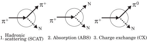
Figure 1: Pion interactions on nuclei. “N” represents any number of nucleons emitted after interactions

The Dual-Use Experiment at TRIUMF (DUET) is intended to improve the precision of pion absorption and charge exchange interaction cross sections on both carbon and water. A scintillator tracker is used for precision studies of pion interaction final states. The experiment is capable of measuring interactions on carbon and water. A limited number of photon detectors were deployed to allow the separation of absorption and charge exchange interactions. In this paper, we present a measurement of the combined absorption and charge exchange cross section ($\sigma_{\mathrm{ABS}+\mathrm{CX}}$) on carbon with significantly improved precision relative to previous measurements.

II Experiment

$\sigma_{\mathrm{ABS}+\mathrm{CX}}$ was measured on a carbon target at 5 different momentum settings between 201.6 MeV/c and 295.5 MeV/c. The ABS and CX events are selected by requiring no observed pion in the final state, therefore a detector with excellent tracking capabilities was essential. The pion interactions were measured within the PIA$\nu$O (PIon detector for Analysis of neutrino Oscillation) detector, which was composed of 1.5 mm scintillating fibers to provide precise tracking and dE/dx measurements of particles in the interaction final state.

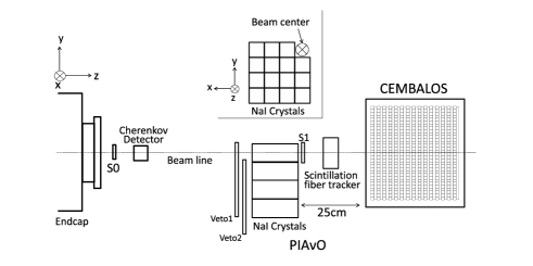
Figure 2: Apparatus layout. Detailed description in the text.

II.1 Beam line and triggers

The experiment took place in the M11 secondary beam line at TRIUMF. Figure 2 shows the overview of the M11 beamline area and the placement of the detectors. A 500 MeV proton beam extracted from the TRIUMF main cyclotron was directed onto a 1 cm carbon target. The pions produced in the target were directed down the M11 beam line by two dipole magnets and focused by a series of six quadrupole magnets. The accelerator facility allowed the possibility to select different pion momenta, and the momentum settings used were 201.6, 216.6, 237.2, 265.5, 295.1 MeV/c. The momentum of the pion beam is measured using CEMBALOS, described in Chapter V.

In addition to pions, the secondary beam also contained protons produced from the target, and muons and electrons resulting from the pion decay chain. The pions were selected using Time-Of-Flight (TOF) measurements and a Cherenkov detector. The TOF of each secondary particle was the difference between the time measured in the Current Transformer (CT), located near the production target, and scintillator counter S1, placed $\sim$15 m downstream of the CT. The CT, S0, and S1 detectors were read out by a VME module (CAEN TDC V1190), and the TOF determined by the difference in TDC counts between S1 and the CT. A Cherenkov counter was placed $\sim$11 cm downstream of the S0 counter, and consisted of a 3.5 cm $\times$ 3.5 cm $\times$ 20 cm bar of Bicron UV-transparent acrylic plastic read out at each end by photomultiplier tubes. The refractive index of the acrylic bar was 1.49, so muons with momentum larger than $\sim$250 MeV/c produced Cherenkov light at angles that were totally internally reflected within the bar, whereas pions of the same momentum produced Cherenkov light at an angle that was largely transmitted. The signals of the two PMTs were read out by a VME module (CAEN ADC V792), and the Cherenkov light for each event was obtained from the sum of the ADC counts of the two PMTs. Figure 3 shows an example of Cherenkov light vs. TOF for $p_{\pi}=$ 237.2 MeV/c. The electron, muon and pion signals are clustered around the left top, middle and right bottom of the plot, respectively. The pion candidates are below the broken line. The purity of pions after this cut is estimated to be larger than 99% for all the momenta settings used in the analysis.

The S0 and S1 scintillator counters were used in coincidence to select low angle charged particles entering the PIA$\nu$O detector.

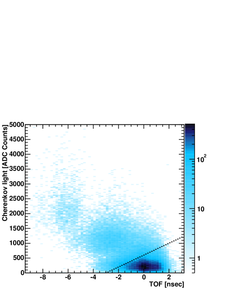
Figure 3: Cherenkov light in ADC counts vs. TOF [nsec] for the beam particle at $p_{\pi}=237.2$ MeV/c setting. The broken line corresponds to the threshold to distinguish pions from muons and electrons.

II.2 Detector description

The PIA$\nu$O fiber tracker consists of 1.5 mm scintillation fibers and is read out by Multi-Anode Photo Multiplier Tubes (MAPMTs). Figure 4 shows the front view of the detector. The pion beam is injected into the center of the detector, where the fibers cross each other perpendicularly to form U and V layers. There are 16 U and 16 V layers, with 32 fibers in each layer for a total of 1024 fibers or channels. The dimension of the region where the fibers cross each other (“fiber crossing region”) is $\sim 5\times 5\times 5$ cm³. The fibers are held together by fiber holders to clip the fibers without glue. The fiber channels are read out by 16 MAPMTs. The structure of the detector, details of the fiber scintillators, the MAPMTs, and the readout electronics are summarized in Table 1.

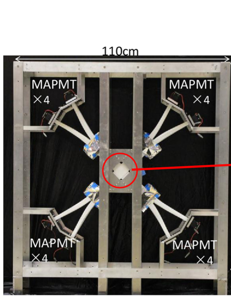
Figure 4: Front view of the fiber tracker detector.

Structure
Dimensions in fiber crossing region	49 mm $\times$ 49 mm $\times$ 51 mm
Dimensions of support structure	110 cm $\times$ 110 cm $\times$ 25 cm
Number of channels	1024
Scintillating fiber
Material	Polystyrene (core), PMMA (clad)
Reflector	EJ-510 ($\sim$ 25 $\mu$m)
Dimensions	0.149 cm $\times$ 0.149 cm $\times$ 60 cm (core + clad)
Clad thickness	2% of core + clad
Emission peak wavelength	450 nm
Decay time	2.8 ns
Attenuation length	$>$ 4 m
MAPMT
Type	Hamamatsu H8804
Anode	8$\times$8 pixels (pixel size: 2$\times$2 mm2)
Cathode	Bialkali (Sb-K-Cs)
Sensitive wavelength	300-650 nm (peak: 420 nm)
Quantum efficiency	12% at $\lambda$=500 nm
Dynode	Metal channel structure 12 stages
Gain	typical 2 $\times$ 106 at 900 V
Crosstalk	$\sim$2% (adjacent pixel)
Readout electronics
Number of ADC channels	1024
ADC pedestal width	less than 0.1 p.e.

Table 1: Specifications of the fiber tracker

The scintillating fibers used are single clad square fibers (Kuraray SCSF-78SJ). The outer surface of the fibers are coated with a reflective coating (EJ-510) which contains TiO₂ to increase the light yield by trapping the light within the fiber and to optically separate the fibers from each other. One end of each fiber is mirrored by vacuum deposition of aluminum which increases by 70% the light yield. The number of nuclei in the fiducial volume of the fiber is estimated from the material and dimension of the fibers, as summarized in Table 2.

Nuclei	Number of nuclei [$\times 10^{24}$]
C	1.518$\pm$0.007
H	1.594$\pm$0.008
O	0.066$\pm$0.004
Ti	0.006$\pm$0.0002

Table 2: The number of nuclei in the fiducial volume of the fiber tracker.

The scintillation light from the fibers is read out by 64 channel MAPMTs which are connected via acrylic connectors. A small fraction of the light from the fibers is transferred to adjacent MAPMT channels which generates crosstalk signals. Adjacent fibers in a layer are connected to non-adjacent MAPMT channels so that crosstalk signals can be separated from the real signal. The crosstalk probability is measured to be $\sim$2% for the adjacent channels. The readout electronics for MAPMTs is recycled from the K2K experimentNitta et al. (2004). Each of the MAPMTs are read out through a front-end board. Signals from the front-end board are digitized by Flash Analog to Digital Converters (FADCs) on the back-end modules mounted on a VME-9U crate.

The high voltage for MAPMTs is tuned in a bench test by measuring 1 photoelectron (p.e.) signals from LED light so that the gain is uniform over all MAPMTs. The high voltage is set to $\sim$950 V, and the typical gain is 60 ADC/p.e. However, it varies by $\sim$23% between MAPMT channels because the gain of the 64 channels within a MAPMT cannot be tuned individually. The measured light yield is $\sim$11 p.e. per fiber for a minimum ionizing particle. The relatively large value of the MAPMT high voltage is necessary to measure the light from the fibers with good resolution. The dynamic range of FADCs is therefore not wide (maximum $\sim$30 p.e.).

Using only the tracker, $\pi^{0}$s from charge exchange events cannot be observed. NaI detectors surrounding the tracker were installed to detect $\gamma$s from the decay of $\pi^{0}$s for separation of absorption and charge exchange events. The apparatus configuration also includes the CEMBALOS (Charge Exchange Measurement By A Lead On Scintillator) detector. This was a scaled-down version of the T2K Fine-Grained Detectors (FGDs) Amaudruz et al. (2012), with removable lead plates sandwiched between scintillator tracking planes to act as another photon detector, together with the NaI detectors. For this analysis, CEMBALOS was used for the evaluation of the systematics for the muon contamination of the beam. The NaI array and CEMBALOS are used in ongoing studies to extract ABS and CX cross sections separately and will be the subject of another paper.

II.3 Detector Simulation

The detector simulation includes a detailed description of the tracker, Cherenkov counter, scintillator counters, and CEMBALOS. The simulation code is based on Geant4 version 9.4 patch 04 Agostinelli et al. (2003). The fiber core, cladding and coating structure of PIA$\nu$O are included in the simulation. The thickness of the coating affects the efficiency to detect a hit above 2.5 p.e. threshold for through-going pions. The efficiency is measured to be $\sim$94% in MC, while it is measured to be 93% in the data.

The misalignment of the fiber layer position is measured from the difference between the measured hit position and the expected hit position for through-going pions. The RMS of the distance from the nominal position is measured to be 80 $\mu m$. The shift is implemented in the simulation by shifting the layer position to the measured position for that layer. The light yield of the fibers in the simulation is tuned so that it agrees with pion through-going data.

The energy deposit for each fiber in the simulation is converted to p.e. by the following procedure.

1. Conversion of energy deposit to photons
   The expected number of photons generated in the fiber ($N_{exp}$) is calculated by multiplying the value of the energy deposit ($E_{dep}$) by a conversion factor, $C_{conv}$ ($\sim$57 p.e./MeV), which is defined channel by channel from the light yield distribution observed in through-going pion data. Thus

   $$N_{exp}=C_{conv}\times E_{dep}$$ (1)

   The saturation of scintillation light is taken into account by using Birk’s formula Birks (1951). The Birk’s constant for our fiber material (polystyrene) is the same as for the FGD Amaudruz et al. (2012).

2. Photon statistics and MAPMT gain
   The photon statistics and the MAPMT gain fluctuation is taken into account. The number of photoelectrons ($N_{P.E.}$) is randomly defined from the Poisson distribution using the mean of the expected number of photons ($N_{P.E.}=\mbox{Poisson(}N_{exp}$)). The observed number of photoelectrons ($N_{obs}$) is obtained by adding a statistical fluctuation term to $N_{P.E.}$:

   $$N_{obs}=N_{P.E.}+\sqrt{N_{P.E.}}\times C_{gain}\times\mbox{Gauss(1)}$$ (2)

   The second term in this equation corresponds to the statistical fluctuation in the multiplication of electrons in the PMT. Gauss(1) is a random value which follows a Gaussian distribution with mean = 0 and sigma = 1. $C_{gain}$ is defined from the charge distribution of 1 p.e. light, which is measured in a bench test by using an LED, and it is defined channel by channel (typically it is $\sim$60%).

3. Electronics
   The number of photoelectrons is converted to ADC counts ($ADC_{raw}$) by multiplying another conversion factor ($C_{conv2}$) with $N_{obs}$. $C_{conv2}$ is measured from the 1 p.e. distribution obtained by LED light, and it is typically $\sim$ 60 ADC counts/p.e.

   The non-linearity of electronics is simulated with an empirical function:

   $$ADC_{obs}=ADC_{raw}/(1+C_{nonlin}\times ADC_{raw})$$ (3)

   where $C_{nonlin}$ is 0.000135/ADC counts. In case the ADC count is greater than 4095, it is set to 4095 to account for saturation in the electronics.

The conversion factor $C_{conv}$ and the non-linearity correction factor $C_{nonlin}$ are obtained by fitting the charge distributions of through-going pions with $p_{\pi}$ = 150 and 300 MeV/c. Figure 5 shows the charge distribution for data, compared with MC after the fit. The charge distribution in MC reproduces the distribution in data very well.

The crosstalk hits are also implemented in the simulation. For each of the “real” hit associated with a particle trajectory, crosstalk hits are generated in adjacent channels in the MAPMTs. The expected number of photons for these crosstalk hits are calculated by multiplying the “real” hit by the crosstalk probability. The crosstalk probability in MC is tuned so that the charge distribution of crosstalk hits in the through-going pion data agree with data. In this tuning, crosstalk hits are selected from the hits which were not on the pion track. The crosstalk probability for adjacent channels in a MAPMT is determined to be $\sim$2%, and the crosstalk between adjacent fibers due to light leaking through the reflective coating is determined to be $\sim$0.8%.

The simulation and calibration procedure for the scintillating bars of CEMBALOS is the same as for the FGD. Figure 6 shows the charge distribution for through-going muons in CEMBALOS for the $p_{\pi}=$ 237.2 MeV/c setting, for data and MC (hereafter, the 237.2 MeV/c data set will be used to show an example). The agreement between data and MC is good except for the low p.e. region. The disagreement in the low p.e. region is due to MPPC noise hits which is not implemented in the simulation. Those noise hits are random and small (typically 1$\sim$3 p.e.). We apply a 5 p.e. threshold in the analysis to reject those hits.

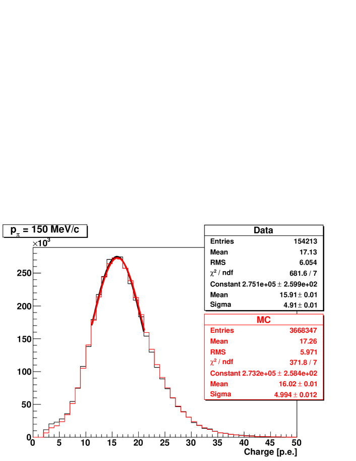
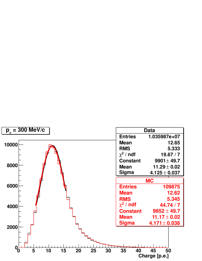
Figure 5: Charge distribution of through-going pions for data and MC, for $p_{\pi}$ = 150 and 300 MeV/c data set. The hits below 2.5 p.e. threshold are not shown in the plots. The fits closely follow each other.

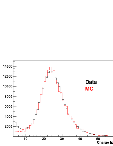
Figure 6: CEMBALOS charge distribution of through-going muons for $p_{\pi}=$ 237.2 MeV/c setting.

The beam position distribution and momentum are measured in data and reproduced in the simulation. In the simulation, pions are generated 1 cm upstream from the S0 trigger. The X and Y position of the generation point and the angular distribution of the beam are tuned so that the measured beam position distribution and the angular distribution of the through-going tracks in the fiber tracker agree between data and MC. A Gaussian distribution is assumed for the initial position distribution and the angular distribution, and the mean and sigma of the distributions are tuned for X and Y. Figure 8 and 8 shows the beam position distribution and angular distribution for data with the 237.2 MeV/c setting compared to the distribution for MC after tuning.

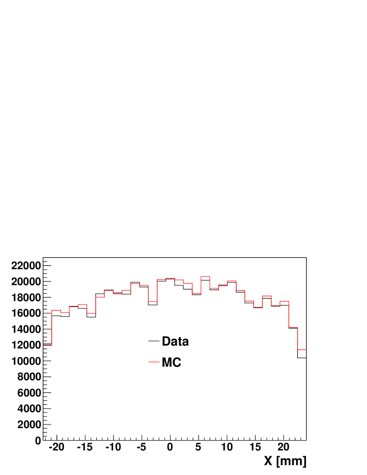
Figure 7: Beam position distribution in X, for the data set with $p_{\pi}=$ 237.2 MeV/c setting. The black (red) histogram shows the distribution for data (MC).

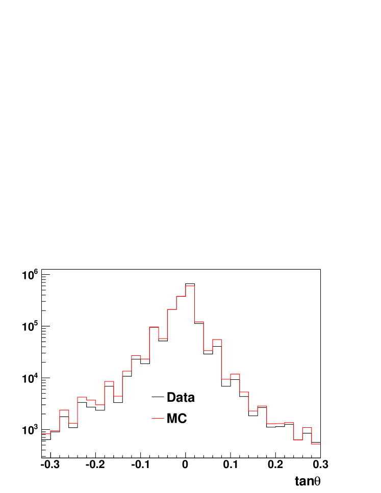
Figure 8: Beam angular distribution in X projection, for the data set with $p_{\pi}=$ 237.2 MeV/c setting. The variable $\theta$ is the angle from horizontal line (X=0). The black (red) histogram shows the distribution for data (MC).

II.4 Data acquisition and event summary

The data acquisition is controlled by using MIDAS (Maximum Integration Data Acquisition System)Ritt et al. (2001). It controls the front-end DAQ programs for each detector, and combines the data to build events.

The data used in the analysis we describe in the following section is for a $\pi^{+}$ beam on a scintillator (carbon) target for five incident momenta (201.6, 216.6, 237.2, 265.5, 295.1 MeV/c) as has been discussed earlier. There were $\sim$ 1.5 million beam triggered events recorded for each momentum settings, except for the 216.6 MeV/c setting where 0.5 Million events were recorded due to limited beam time.

III Event selection

III.1 Event reconstruction

As an illustration of the reconstruction, an ABS candidate event in the data is shown in Figure 9 in the UZ projection where Z is the direction of the beam. The upstream horizontal (blue) track is identified as a pion (“pion-like” track). The other tracks (green and pink) are “proton-like” tracks produced by nuclei receiving energy from the incident $\pi^{+}$.

We describe the track reconstruction procedure in the following section.

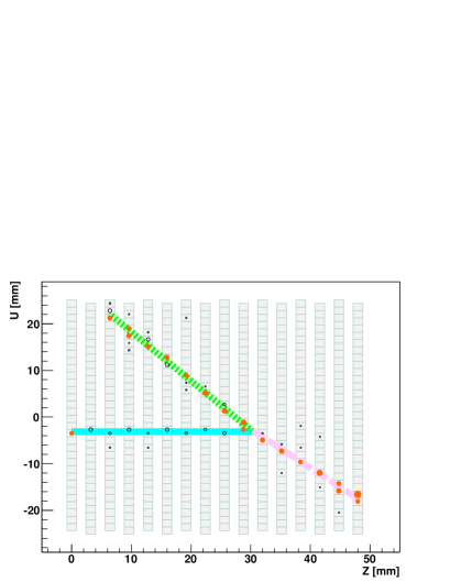
Figure 9: Example of ABS candidate event in data ($p_{\pi}=$237.2MeV/c). The filled circles (red) correspond to the large hits ($>20$ p.e.), the crosses correspond to the hits identified as crosstalk hits and the thick lines (blue, green and red) correspond to reconstructed tracks.

The first step of the event reconstruction is the conversion from ADC count to the number of photo-electrons, followed by an electronics non-linearity correction. The typical number of p.e. is $\sim$ 11 p.e./hit for minimum ionizing particles, and only the hits above 2.5 p.e. are used in the track reconstruction. The efficiency to detect a hit for charged particles passing through the layer is $\sim$93%, where the inefficiency is caused by the inactive region of the fiber. To minimize the effect of the inactive region the positions of the fiber layers are shifted relative to each other, as shown in Figure 9.

In the track reconstruction algorithm, the candidate hits and crosstalk hits are treated differently. The crosstalk hits usually have smaller p.e. and they are associated with hits with larger p.e. Hence when there is a hit with a large p.e. ($>$ 20), the hits with smaller p.e. ($<$ 10) in the adjacent MAPMT channels are identified as crosstalk hits. The tracks are reconstructed in U and V layers individually, and then combined to make 3D tracks according to the following procedure.

1. Incident track search:
   Track candidates are identified by searching for hits on straight trajectories. For the incident track, the straight lines are required to start from the upstream-most layer, and the angle of the lines are required to be nearly horizontal (0 $\pm$ 4 degrees). Starting from the hits in the upstream-most layer, hits on the straight line are searched for in the downstream layers. Hits within two fiber-widths are included for the track candidate, with the process continuing towards subsequent layers until no such hits are found. At least 3 hits are required to make a track. The hits on the incident track are required to be not large ($<$ 20 p.e.), so that the hits from a secondary proton track are not included. In case the hits are large or identified as cross talk, it is not used in the $>$ 3 hits requirement, but the hit tracing does not stop. When there are multiple incident track candidates, the longest track is selected.

2. Interaction vertex search:
   The end position of the incident track is selected as a temporary interaction vertex point. Then a search is conducted for a best vertex position around the temporary vertex in $\pm$ 3 layers and $\pm$ 1 fiber region, where the best vertex position is defined as the position where the largest number of hits can be traced. The procedure to trace the hits is the same as that for the incident track, except for the horizontal track requirement and small hit ($<$ 20 p.e.) requirement. The tracks traced from the best vertex position to the subsequent layers are selected as final tracks.

3. Combining the 2D tracks into a 3D track:
   If the track ends of the 2D tracks in the U and V projections agree, the 2D tracks are combined to form a 3D track. The track end positions may not agree when the particle escapes the fiber crossing region and leaves hits in only one projection. Otherwise the track end position is required to agree within $\pm$ 2 layers. The Z position of the interaction vertex is defined as the average Z position in two projections. The event is rejected in the event selection if the Z position difference between two projections are greater than 4.9 mm.

Comparing the reconstructed track with the true trajectory in the MC, the position resolution of the interaction vertex is evaluated to be $\sim$ 1 mm in U and V, and $\sim$ 2 mm in Z (Figure 10 a,b,c). The angular resolution of the reconstructed track is evaluated to be $\sim$ 3 degree (Figure 10 d).

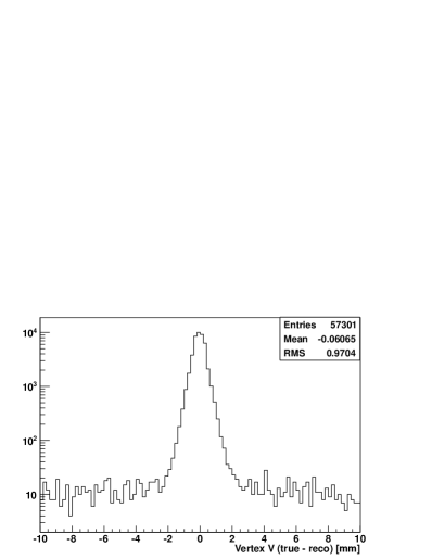
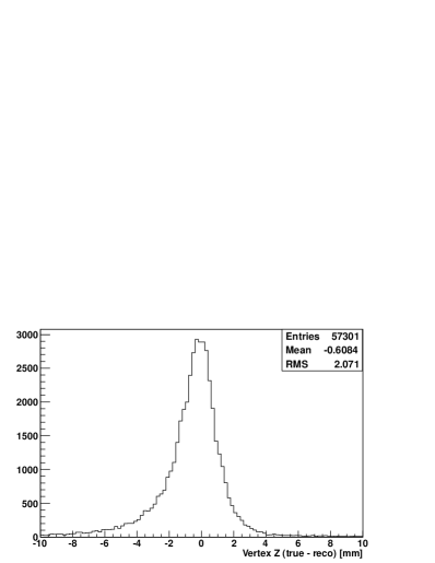
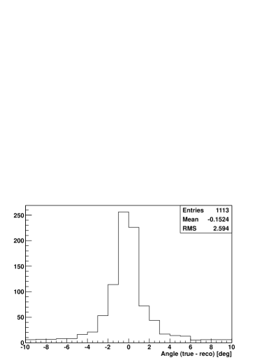
Figure 10: Difference between the true and reconstructed vertex position in U, V and Z, and the true and reconstructed angle.

For each track, we calculate the deposited charge per track length, dQ/dx, obtained by dividing the total charge deposit by the total length of the track. The dQ/dx is used for identifying the particle types in the event selection. For large hits ($\sim$30 p.e.), the measured charge can be smaller than the actual charge because of the electronics saturation effect. The effect of saturation becomes significant when the path length within a fiber is long, resulting in a large charge deposit. Since the angle relative the fiber orientation in the U and V projections are different, the path length in each view will generally be different. In order to minimize the saturation effect, we calculate the dQ/dx from the projection with the shorter path length per fiber.

III.2 Event selection criteria

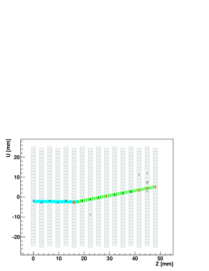
Figure 11: Example of pion scattering candidate event in data ($p_{\pi}=$237.2MeV/c). The track (blue) in the upstream side is identified as the incident pion track, and the track in the downstream side (green) is identified as a scattered pion track.

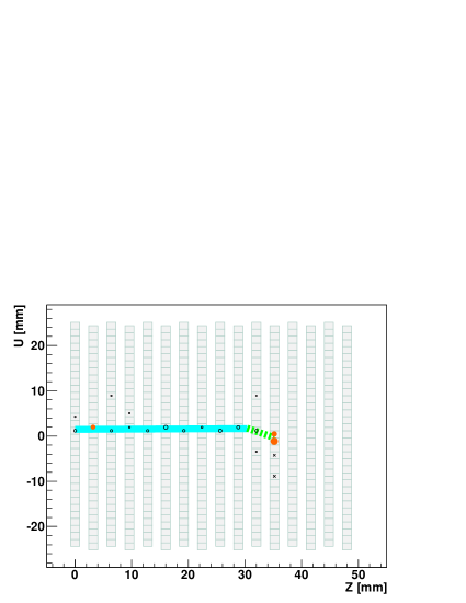
Figure 12: Example of CX candidate event in data ($p_{\pi}=$237.2MeV/c). The track in the upstream side (blue) is assumed to be the incident pion track, and the track in the downstream side (green) is assumed to be a proton track from CX interaction.

Examples of ABS, CX, SCAT event candidates are shown in Figure 9, 12, and 11 respectively. The SCAT events can be readily identified by the outgoing pion track, in contrast to the ABS and CX events where the incident pion track terminates and may lead to the emission of proton tracks. CX events are identified by a coincident signaling in the NaI crystals resulting from the outgoing photons from the decay of the $\pi^{0}$ from the charge exchange reaction. As a result, ABS+CX events are selected by requiring no $\pi^{+}$ in the final state, where final state tracks are identified as all reconstructed tracks in the event apart from the incident pion, whereas SCAT events have a pion track in the final state in addition to any protons that may be produced in the interaction. ABS events typically have one or two protons in the final state, whereas a CX event will usually have zero or only one proton.

The ABS + CX event selection is considered in further detail below.

1. Good incident $\pi^{+}$
   This selection consists of three requirements. First, we require that the incident particle is a charged pion. We apply a cut in the Cherenkov light vs. TOF distribution, as explained in Section II.1 (except for the 201.6 MeV/c data set, in which we used the TOF distribution only).

   Second, we impose requirements to make sure that a straight track, normal to the incidence plane, exists. For this we require hits on the first, third and fifth layers, and in the same fiber position (i.e. same U, V position) in both the U and V projections (see Figure 13). Only a horizontal straight track passes this cut. The background muons originating from the decay of pions are rejected by this cut because in most of cases the angle of these muons are shifted with respect to the beam axis.

   Third, we require the incident track to enter the fiducial volume (FV). The FV is shown as the broken lines in Figure 13 and 14. Figure 14 shows the X, Y position distribution of the incident beam. The hexagonal shape corresponds to the region where the S1 trigger overlaps with the fiber crossing region. Because the reconstruction algorithm requires at least 3 hits to reconstruct a track, the fiducial volume is defined to be $\geq$ 3 fibers (3 layers) from the upstream edge of the fiber crossing region. The X, Y position of the incident track is required to be inside the X-Y plane of the FV.

2. Vertex in the FV
   After the Good incident $\pi^{+}$ selection, $\sim$90% of the remaining events are through-going pion events. The events with pion interactions are selected by requiring a reconstructed vertex inside the FV. With this cut we attempt to reject not only through-going events but also pion scattering events with a very small scattering angle (“small angle” event). To identify these events, we count the number of hits inside or outside $\pm$ 2 fibers of the incident U, V position. “Small angle” events look very similar to through-going pion events, but can be rejected by requiring no reconstructed hits outside the 2 fiber region and $\geq$25 hits inside the 2 fiber region, with at least 2 hits in the last three layers.

3. No final $\pi^{+}$ track
   In this selection we require there be no $\pi^{+}$ in the final state. The pion tracks are distinguished from proton tracks by applying a dQ/dx cut. Figure 15 shows an example of dQ/dx distributions for $p_{\pi}=$ 237.2 MeV/c for data and MC. There are six plots corresponding to six different angular regions ($0^{\circ}<\theta<30^{\circ},30^{\circ}<\theta<60^{\circ},...150^{\circ}<\theta<180^{\circ}$), where $\theta$ is the angle of the reconstructed track with respect to the beam direction. The histograms for MC are normalized by the number of incident pions. The color of the histograms represents the interaction types. The vertical broken line represents the threshold to distinguish pions and protons. Because the dQ/dx distribution varies with angle and incident momentum, different thresholds are set for each combination of outgoing track angle and incident momentum. If any of the reconstructed tracks except the incident track is found to have dQ/dx below the threshold, then that track is identified as a charged pion, and the event is not selected.
   In order to identify the scattered pion track which is reconstructed only in U or V projection, the dQ/dx cut is also applied for the 2D tracks. For the 2D tracks, the dQ/dx is calculated by using the track length projected in 2D, which is shorter than the actual 3D track length. Therefore, the dQ/dx is overestimated for 2D tracks. However, we apply the same dQ/dx threshold for both 3D and 2D tracks, to avoid mis-identifying ABS or CX events as pion scattering events.

Figure 13: Illustration of the Good incident $\pi^{+}$ cut requirement. The broken line represents the boundary of the fiducial volume

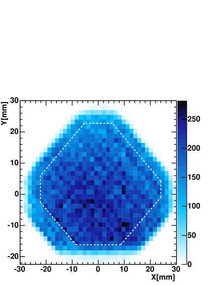
Figure 14: The X-Y view of incident beam position distribution. The white broken line represents the boundary of the fiducial volume

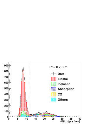
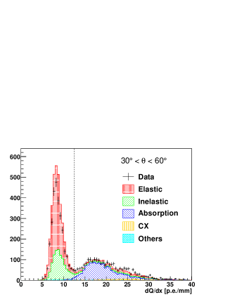
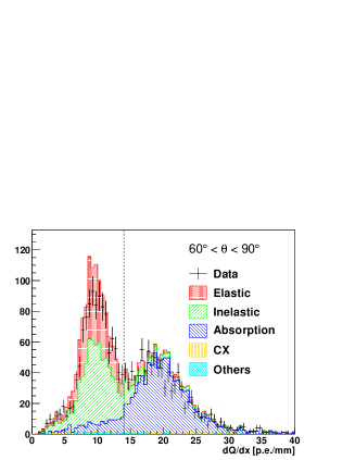
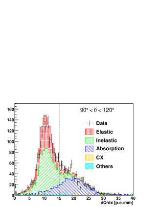
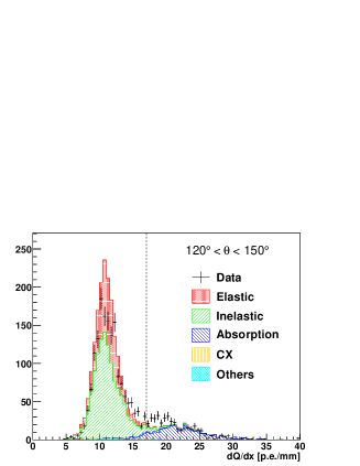
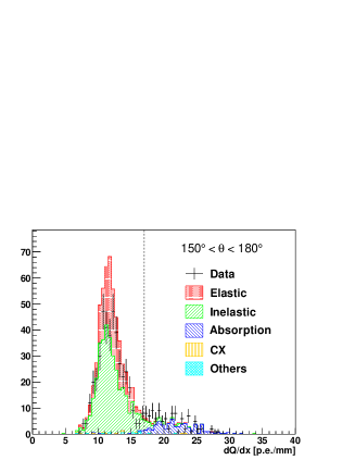
Figure 15: dQ/dx distribution in six different angular regions for $p_{\pi}=$ 237.2 MeV/c for data and MC. The dotted vertical lines represent the threshold to distinguish pions (left of the line) and protons. For multiple track events, only the smallest value of dQ/dx among the tracks is filled in the histogram. The events in the “Others” category is mainly from events with pions decaying in flight and Coulomb scattering events.

III.3 Selection efficiencies

The number of selected events after each stage of the cuts is summarized in Table 3. There are $\sim$7000 events in data after the event selection, except for the 216.6 MeV/c data set in which the number of incident pions is smaller due to the limited data taking time. The efficiency to select ABS or CX events which occurs inside the fiducial volume is estimated to be $\sim$79%, and the purity of ABS + CX events in the selected sample is estimated to be $\sim$73%. The details of the MC simulation and comparison with data after event selection are explained in Sec IV.

	201.6 MeV/c		216.6 MeV/c		237.2 MeV/c		265.5 MeV/c		295.1 MeV/c
Cut	Data	MC	Data	MC	Data	MC	Data	MC	Data	MC
Good incident $\pi^{+}$	273625		67164		276671		238534		282611
Vertex in FV	17522	18895.9	4833	5118.8	21861	22932.1	20567	20895.1	24327	24136.7
No final $\pi^{+}$	6797	6331.2	1814	1695.9	7671	7619.0	6772	7005.1	7289	7491.1
Efficiency [%]	79.0		79.6		79.9		79.2		77.1
Purity [%]	73.0		73.3		73.1		73.5		73.1

Table 3: The number of events after each stage of the cut. The numbers for MC are normalized by the numbers of good incident pion events in data.

III.4 Background

When pions are scattered, the scattered pion tracks are not always well reconstructed, particularly when the pion is scattered nearly 90 degrees and the track passes between fiber layers. Also, due to finite dQ/dx resolution, pion tracks are sometimes misidentified as protons. These background events pass the event selection. Although the cross section of pion elastic scattering in the MC is tuned to results from previous experiments, a linear interpolation of the data points from the previous measurements does not perfectly reproduce the actual cross section. The estimation of the uncertainty for the number of predicted background events is described in section V.1.9.

IV Simulation and tuning of physics models

The hadronic interaction of the pions with a nuclei is simulated by using the list of physics models called “QGSP-BERT”. For the elastic scattering, it uses a model called “hElasticLHEP” based on a simple parametrization of the cross section. The inelastic scattering (INEL), ABS and CX are included in the inelastic process, which are simulated using the Bertini Cascade modelHeikkinen et al. (2003).There are also other processes, namely double charge exchange and hadron production, but the cross sections for those interactions are negligibly small in the pion momentum range in this experiment.

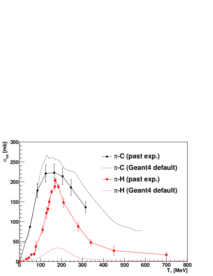
Figure 16: Comparison of elastic inclusive cross section between the previous experiments (summarized in Table 4) and the default Geant4. The cross sections are plotted as a function of pion kinetic energy.

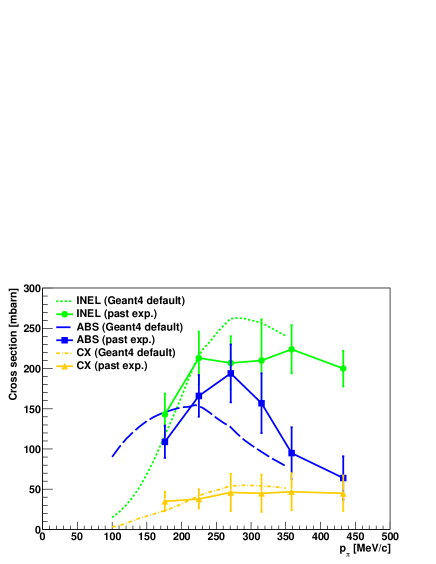
Figure 17: Comparison of inelastic inclusive cross sections between the previous experiment Ashery et al. (1981) and the default Geant4. The cross sections are plotted as a function of pion momentum.

The $\pi^{+}-$C and $\pi^{+}-$H elastic cross sections and differential cross sections (d$\sigma/d\theta$) were tuned by interpolating the data points from previous measurements. The inclusive $\pi^{+}-$C inelastic scattering, ABS and CX cross sections were also tuned. Figure 16 and 17 shows the comparison of the cross sections between the previous experiments and the default Geant4 MC data, for elastic and inelastic processes. There are disagreements between Geant4 cross section (ver9.4, QGSP-BERT) and the measurements from the previous experiments, especially for $\pi-$H elastic scattering process. Table 4 summarizes the data from previous experiments that we used for the tuning. The momentum of pions after inelastic scattering is predicted using the NEUT cascade model Hayato et al. (2002) because there is no available data.

Measurement	Kinetic energy (MeV)	Reference
$\pi-$C inclusive	85, 125, 165, 205, 245, 315	D. Ashery et al. Ashery et al. (1981)
(elastic, inelastic, ABS and CX)
$\pi-$C elastic inclusive	49.9	M. A. Moinester et al. Moinester et al. (1978)
$\pi-$H elastic inclusive	33, 44, 56, 70	S. L. Leonard et al. Leonard and Stork (1954)
	78, 110, 135	H. L. Anderson et al. Anderson et al. (1953)
	165	H. L. Anderson et al. Anderson and Glicksman (1955)
	128, 142, 152, 171, 185	J. Ashkin et al. Ashkin et al. (1954)
210, 280, 340, 450, 700	Lindenbaum et al. Lindenbaum and Yuan (1955)
$\pi-$C elastic differential	40	M. Blecher et al. M.Blecher et al. (1979)
	50	R. R. Johnson et al. R.R.Johnson et al. (1978)
	67.5	J. F. Amann et al. Amann et al. (1981)
	80	M. Blecher et al. Blecher et al. (1983)
	100	L. E. Antonuk et al. Antonuk et al. (1984)
	142	A. T. Oyer et al. Oyer (1976)
	162	M. J. Devereux et al. Devereux (1979)
180, 200, 230, 260, 280	F. Binon et al. F.Binon et al. (1970)
$\pi-$H elastic differential	29.4, 49.5, 69	J. S. Frank et al. J.S.Frank et al. (1983)
	69	Ch. Joram et al. Joram et al. (1995)
	87, 98, 117, 126, 139	J. T. Brack et al. J.T.Brack et al. (1986)
	87, 98, 117, 126, 139	J. T. Brack et al. J.T.Brack et al. (1995)
166.0, 194.3, 214.6, 236.3, 263.7, 291.4	P. J. Bussey et al. P.J.Bussey et al. (1973)

Table 4: List of data sets used for cross section tuning in simulation.

Figure 18 and 19 shows the number of tracks and angular distribution for the reconstructed tracks before and after the tuning, for $p_{\pi}$ = 237.2 MeV/c data set. The No final $\pi^{+}$ cut is not applied for these plots. The forward angle multiple track events increased after the tuning, mainly due to the increase of $\pi-$H elastic cross section. The agreement between data and MC is much better with the tuning, although there are still small disagreements because the linear interpolation does not perfectly reproduce the data. The difference between data and MC is included in the systematic error.

Figure 20 shows the angular distribution of the reconstructed tracks before and after applying the No final $\pi^{+}$ cut, for 201.6, 237.2 and 295.1 MeV/c data sets. In case there are multiple tracks in the final state, only the track with the smallest value of dQ/dx is selected to fill the histograms in these plots. Figure 21 shows the number of tracks distribution before and after applying the No final $\pi^{+}$ cut. After applying the No final $\pi^{+}$ cut, the fraction of ABS and CX events increase, and the agreement between data and MC becomes worse. This is expected, because the kinematics of the final state particles for ABS and CX interactions are not tuned. The event selection efficiency is affected by this difference, so it is taken into account in the systematic error.

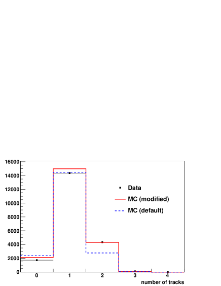
Figure 18: The number of reconstructed tracks for data, and the MC before and after tuning, for $p_{\pi}=$237.2 MeV/c setting. The No final $\pi^{+}$ cut is not applied.

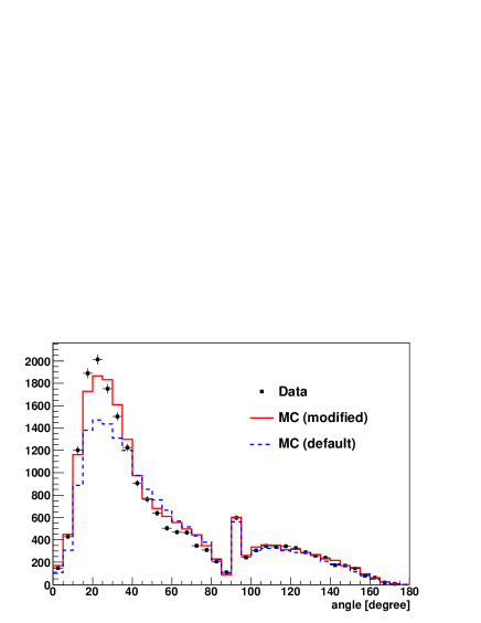
Figure 19: The angular distribution of reconstructed tracks for MC before and after tuning, and for data, for $p_{\pi}=$237.2 MeV/c data set. The No final $\pi^{+}$ cut is not applied.

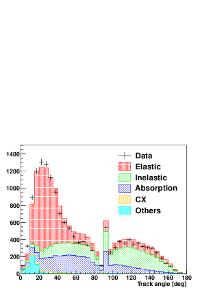
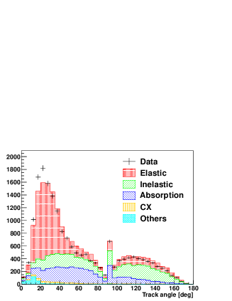
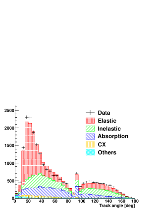
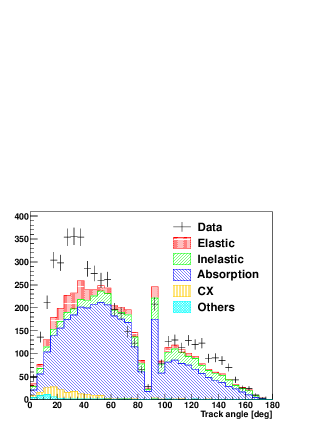
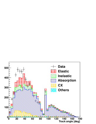
Figure 20: Angular distribution of the reconstructed tracks in the final state for $p_{\pi}$ = 201.6 (left), 237.2 (center) and 295.1 (right) MeV/c data, before (top) and after (bottom) applying No final $\pi^{+}$ cut. When the true track angle is close to 90 degrees, the track reconstruction algorithm tends to reconstruct the track exactly at 90 degrees, so the number of events in the bin corresponding to 90 degrees is larger than the neighboring bins.

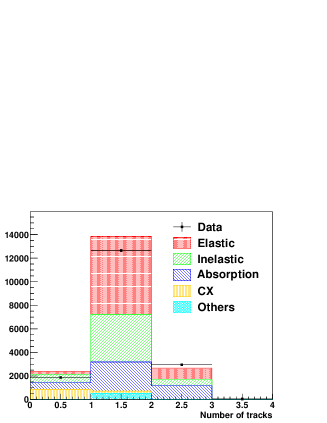
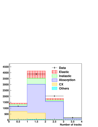
Figure 21: Distribution of number of reconstructed tracks in the final state, for 201.6 (left), 237.2 (center) and 295.1 (right) MeV/c data sets, before (top) and after (bottom) applying No final $\pi^{+}$ cut.

V Cross-section and error analysis

After the event selection described above, the cross section is obtained by adding the corrections for muon contamination and interaction on other nuclei using the following formula,

$$\sigma_{\mathrm{ABS}+\mathrm{CX}} =\sigma_{\mathrm{ABS}+\mathrm{CX}}^{pred}\times\frac{N_{\mathrm{data}}-N_{\mathrm{BG}}^{pred}}{N_{\mathrm{sig}}^{pred}}$$ (4)

$$\times\frac{1-R_{\mathrm{TiO}}^{data}}{1-R_{\mathrm{TiO}}^{\mathrm{MC}}}\times\frac{1}{1-f_{\mu}}$$

where $f_{\mu}$ is the fraction of muons in the beam, $R_{\mathrm{TiO}}^{data}$ and $R_{\mathrm{TiO}}^{\mathrm{MC}}$ are the fraction of ABS and CX events on Ti or O after the event selection for data and MC, shown in Table 7. As mentioned earlier, the outer surface of the fibers has a reflective coating which contains TiO₂, hence the expected fraction of ABS and CX events in Ti or O in the data must be corrected. $R_{\mathrm{TiO}}^{data}$ is estimated from the number of Ti and O nuclei (see Table 2) and the ABS and CX cross-sections for these nuclei, which are calculated by interpolating the measured cross sections by a previous external experimentAshery et al. (1981).

V.1 Estimation of the systematic errors

In this section, we describe in detail the estimation of the systematic errors in the pion interaction measurement, which are summarized in Table 5.

	$p_{\pi}$ at the fiber tracker [MeV/c]
	201.6	216.6	237.2	265.5	295.1
Systematic errors
Beam profile	0.9	1.2	1.0	0.6	1.2
Beam momentum	1.6	1.7	0.7	0.8	1.4
Fiducial Volume	1.1	3.9	1.4	1.2	1.3
Charge distribution	2.4	2.2	2.6	2.6	2.9
Crosstalk probability	0.3	0.3	0.3	0.2	0.4
Layer alignment	0.5	0.8	1.1	1.0	1.4
Hit efficiency	0.3	0.3	0.2	0.4	0.3
Muon contamination	0.5	0.8	0.9	0.3	0.2
Target material	0.8	0.9	0.9	0.8	1.0
Physics models (selection efficiency)	2.8	4.9	2.9	4.8	3.7
(background prediction) +	2.8	1.8	2.4	2.3	3.3
$-$	6.1	3.7	3.6	1.5	1.9
Subtotal +	5.2	7.3	5.2	6.3	6.4
$-$	7.5	8.0	5.9	6.0	5.8
Statistical error (data)	1.7	3.1	1.7	1.8	1.7
Statistical error (MC)	0.1	0.1	0.1	0.1	0.1
Total +	5.5	8.0	5.5	6.6	6.7
$-$	7.7	8.6	6.2	6.3	6.1

Table 5: Summary of the statistical and systematic errors in percentage.

A large part of them are estimated by changing the relevant parameters in the MC. Those systematic errors are defined as the difference between the cross section obtained with the nominal MC and the changed MC.

V.1.1 Beam profile and momentum

The properties of the beam are precisely measured in through-going pion data by using beam position distribution, stopping range distribution and charge distribution. The uncertainty of the momentum is less than 1 MeV/c, and the uncertainties on the beam centre position and RMS are $\sim$ 1 mm or less. The systematic error for the cross section is evaluated by changing the momentum, the center position and the spread of the beam in MC within their uncertainty.

V.1.2 Fiducial volume

An interaction which occurred inside the fiducial volume is sometimes reconstructed outside the fiducial volume, or vice versa. The fiducial volume systematic error accounts for the uncertainty of this effect. The size of this effect becomes significant when the definition of the FV becomes smaller. Therefore the systematic error is estimated by reducing the size of FV by $\sim 20\%$ and calculating the difference in the cross section obtained with nominal FV and reduced FV.

V.1.3 Charge distribution and crosstalk probability

This systematic error is calculated by changing $C_{conv}$, $C_{fluc}$, $C_{nonlin}$ and the crosstalk probability in MC within their uncertainty. The center values and the uncertainties of $C_{conv}$ and $C_{nonlin}$ are evaluated by fitting the charge distribution in through going pion data obtained at 150 and 295.1 MeV/c settings. The value of $C_{fluc}$ is defined from the charge distribution of 1 p.e. light. The uncertainty of $C_{conv}$, $C_{fluc}$ and $C_{nonlin}$ are $\sim 2\%,\sim 6\%$ and $\sim$ 18%, respectively. The crosstalk probability is also estimated by using through-going pion data, and the uncertainty is $\sim$ 3%.

V.1.4 Layer alignment

The shift in the position of fiber layers from the nominal position is measured using through-going pion data, as mentioned in Section II.3. The effect of the uncertainty in the layer position on the cross section measurement is estimated by changing the layer position in MC to nominal and checking the difference in the measured cross section.

V.1.5 Hit efficiency

The efficiency to find a hit above 2.5 p.e. threshold for the charged particles passing through the layer is measured in through-going pion data. The efficiency for data was $\sim$ 93%, while it was $\sim$ 94% for MC, so the uncertainty is assumed to be $\sim$ 1%. The effect on the cross section is estimated by randomly deleting the hits in MC with $\sim$ 1% probability and checking the difference in the resulting cross section.

V.1.6 Muon contamination

The uncertainty of muon contamination in the pion beam directly affects the normalization of the measured cross section. For the 265.5 and 295.1 MeV/c data sets, the fraction of muons in the beam is measured in through-going particle data using CEMBALOS. The absolute error is 0.3 and 0.2%, respectively. For the other data sets, the fraction of muons is estimated from the TOF vs. Cherenkov light distribution (Figure 3). The distribution is projected on the axis perpendicular to the threshold line, and the fraction of events above threshold is calculated assuming that the distribution follows Gaussian distribution. However, 0.8$\sim$0.9% of pions which decay just before reaching the fiber and identified as incident pion in the event selection. Those pions may not be correctly counted with this method. Even though the simulation takes into account those pions, to be conservative, 0.8$\sim$0.9% is assigned for the systematic error.

V.1.7 Target material

The number of C, H, O and Ti nuclei in the fiber detector is calculated from the dimension and the weight of the fibers. The number of C nuclei is estimated to be 1.518$\pm$0.007$\times$10²⁴, and this directly affects the normalization of $\sigma_{\mathrm{ABS}+\mathrm{CX}}$. There is also an uncertainty in the number of ABS + CX events on O and Ti, which is estimated to be to be 11$\sim$14% from the interpolation of the previous experiment Ashery et al. (1981).

V.1.8 Selection efficiency due to physics models

The uncertainty in the physics model in MC affects the efficiency to select ABS and CX events. This uncertainty corresponds to the uncertainty of $N_{\mathrm{sig}}^{pred}$ in Eq. 4. Table 6 summarizes the fractional uncertainty of $N_{\mathrm{sig}}^{pred}$ arising from four sources of uncertainties occurring from the modelling of the physics processes within the MC.

Each of them are described in the following text.

	$p_{\pi}$ at the fiber tracker [MeV/c]
Error source	201.6	216.6	237.2	265.5	295.1
Forward / Backward protons	0.4	3.2	1.4	3.2	1.8
dQ/dx resolution	2.7	3.6	2.2	3.4	1.7
High momentum protons	0.5	0.9	1.2	0.9	2.5
$\gamma$ conversion	0.3	0.6	0.8	0.4	0.6
Subtotal	2.8	4.9	2.9	4.8	3.7

Table 6: Summary of the physics model systematic errors related to event selection efficiency (in percentage).

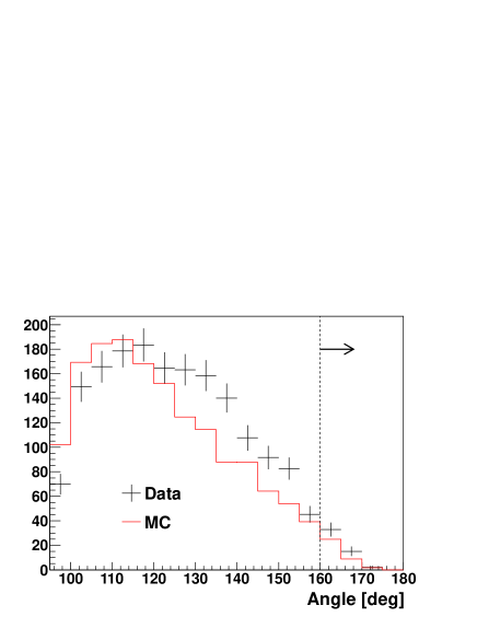
Figure 22: Angular distribution of the backward going proton-like track for data and MC, for ABS and CX events, for $p_{\pi}=$ 237.2 MeV/c setting. For each event, a proton-track with largest angle is selected and filled in the histogram. The ABS + CX event selection is applied for this plot. The background component (SCAT) is subtracted according to the prediction in MC, and the histograms are normalized by the number of events after subtraction.

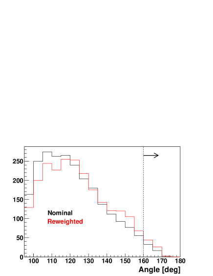
Figure 23: Angular distribution of the backward going proton-like track for nominal and reweighted MC, for ABS and CX events, for $p_{\pi}=$ 237.2 MeV/c setting.

Forward and backward going protons

When a forward going ($\theta<$ 20^∘) proton track exists, the position of the interaction vertex may be wrongly reconstructed downstream of the actual vertex. When a backward going ($\theta>$ 160^∘) proton track exists, the incident track may not be identified because it overlaps with the proton track. Therefore, the event selection efficiency is affected by the fraction of ABS and CX events associated with forward/backward proton tracks.

Figure 22 shows the angular distributions for backward going proton-like tracks for data and MC with $p_{\pi}=$ 237.2 MeV/c setting. The data is 1.4 times larger in the region above $\theta>$ 160^∘. In the case of forward going proton-like tracks the data is found to be 1.3 times larger in the region below $\theta<$ 20^∘. The effect of this difference to the event selection efficiency is estimated by using a re-weighted MC sample in which the fraction of events with a forward/backward going proton track is increased to reproduce the data. Figure 23 shows the angular distribution of proton-like tracks for nominal and re-weighted MC. The event selection efficiency is compared between nominal and the re-weighted MC, and the difference is assigned as a systematic error. The error varies from 0.4% to 3.2% depending on the data sets because the agreement between data and MC is different for different data sets.

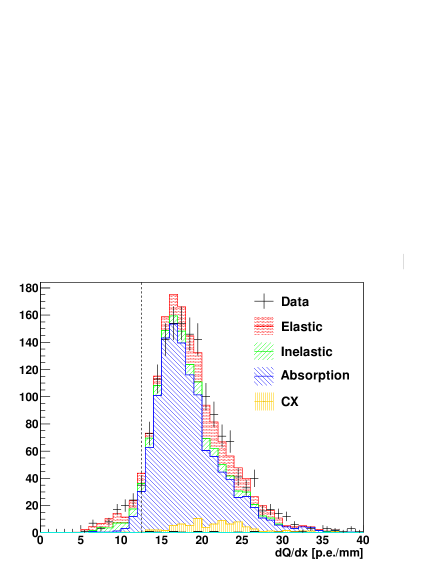
Figure 24: Example of dQ/dx distribution for $30^{\circ}<\theta<60^{\circ}$ after event selection, for the projection which was not used for calculating dQ/dx in No final $\pi^{+}$ cut, for the data set with $p_{\pi}=$237.2MeV/c setting. The broken line shows the threshold to distinguish pion-like tracks and proton-like tracks.

dQ/dx resolution

Events in which a proton track is misidentified as a pion by the dQ/dx cut due to the finite dQ/dx resolution are rejected by the No final $\pi^{+}$ cut. The probability to misidentify a proton track as a pion track is estimated from the probability to pass dQ/dx cut in one projection (U or V) but not in the other projection. As mentioned in Section III.2, the dQ/dx is calculated from U or V projection and not from both projections, to minimize the effect of saturation of the electronics. Figure 24 shows an example of the dQ/dx distribution in one projection, when the dQ/dx is required to be above threshold in the other projection. The probability to pass the dQ/dx cut in one projection but not in the other projection is compared between data and MC. For example, in Figure 24, the fraction of events below the threshold is 5% for data, while it is 4% for MC. Therefore, 25% error is applied for the number of ABS and CX events with proton-like track reconstructed in this angular region, at this momentum. Although this error is not small, the effect on the total cross section is not significantly large because the efficiency of the dQ/dx cut is large ($\sim$ 90%) and the number of ABS or CX events which do not pass this cut is small.

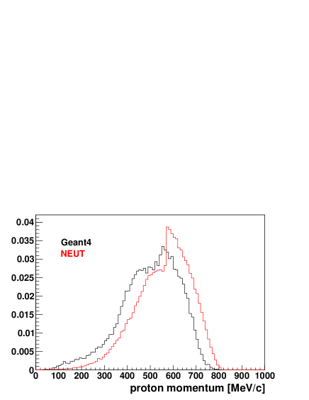
Figure 25: The predicted momentum distribution of protons from the ABS events, for Geant4 (black) and NEUT (red), for $p_{\pi}=$ 295.1 MeV/c. The histograms are normalized by number of ABS events.

High momentum protons

A small fraction of ABS events have very high momentum protons ($>$ 600 MeV/$c$) in the final state which can not be distinguished from pions. Figure 25 shows an example of the predicted momentum distribution of protons in the final state of ABS events for Geant4 and NEUT, for $p_{\pi}=$ 295.1 MeV/c case. A large difference is observed between two different models and the difference in the fraction of events above 600 MeV/c is assigned as the error for the number of high momentum proton events. Because the number of such events is small, the error for those events does not significantly affect the error in the cross section.

Photon conversions

When the $\gamma$-rays from $\pi^{0}$ decays in CX events are converted to electrons and positrons, these electron tracks may be misidentified as pion tracks. These CX events are rejected by the No final $\pi^{+}$ cut. The uncertainty for the number of these events are estimated from uncertainty in the fraction of CX events and the uncertainty in $\gamma$ conversion probability. The uncertainty in the fraction of CX events is $\sim$ 50% Ashery et al. (1981), and the uncertainty of $\gamma$ conversion probability is $\sim$ 5% Cirrone et al. (2010). The systematic errors for the cross section is small because the fraction of these events is only $\sim$ 2% of the total number of ABS and CX events.

V.1.9 Background estimation from physics models

Pion scattering events are misidentified as ABS and CX, when the scattered pion tracks are not identified properly. For example, when the pion scattering angle is close to 90 degrees, the pion track may not be reconstructed in one of the two projections, since it may not pass through enough fiber layers. Also, due to finite dQ/dx resolution, pion tracks are sometimes misidentified as protons. The tuning based in a linear interpolation of data points from the previous measurements does not perfectly reproduce the actual cross section. The uncertainty for the number of predicted background events is estimated in four different categories, as described in the following text.

Pion hadronic scattering

The number of pion scattering events is compared between data and MC in a background enhanced sample. For this data sample, $\pi$-like tracks are required in the event selection instead of applying No final $\pi^{+}$ cut.

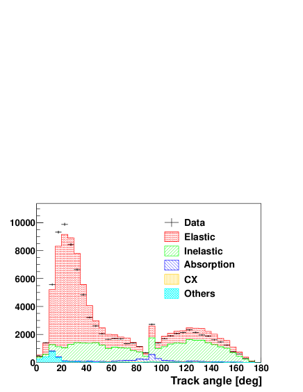
Figure 26: Angular distribution of $\pi$-like tracks for data and MC with $p_{\pi}=$ 237.2 MeV/c setting. The histograms are normalized by number of incident pions in data.

Figure 26 shows the angular distribution for $\pi$-like tracks, compared between data and MC. The angular distribution is divided into six different regions: 0-30, 30-60, 60-100, 80-100, 100-130 and 130-160 degree. The definition of these are different from the angular regions used in the dQ/dx cut because the region around 90 degree is important and should not be divided into two regions. For each region, the difference between data and MC is assigned as the error for the number of predicted background events in that region.

Back-scattered pions

For the angular region above 160 degrees, a special data sample is prepared in order to compare the difference between data and MC. When the scattered angle is near 180 degree, the scattered pion track overlaps with the incident pion track. In most cases the overlap happens in only one projection, but not in both projections. For those back-scattering events, the dQ/dx for the overlapped incident track is large, and the scattered pion track is not reconstructed properly in one of the two projections.

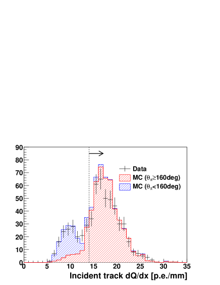
Figure 27: Example of dQ/dx distribution for incident track for the data set with $p_{\pi}=$ 237.2 MeV/c setting, after requiring $\pi$-like track in only one of the two projections. The histograms are normalized by number of incident pions.

Figure 27 shows an example of the dQ/dx distribution for incident tracks, when a $\pi$-like track (dQ/dx $<$ 15 p.e. / mm) is reconstructed in only one projection. The back-scattered pion data sample is selected by requiring dQ/dx $>14$ p.e./mm in this plot. The difference between data and MC is assigned as the error for the predicted number of back-scattered pion background events.

Multiple interaction

Scattered pion tracks may not be reconstructed properly when they interact again in the fiber tracker. For example, if a pion is absorbed right after being scattered, the scattered pion track will be too short to be reconstructed. Among all of the pion scattering events that are misidentified as ABS or CX, $\sim$ 30% of those are due to multiple interactions like this. The uncertainty of the number of events for this type of background events is estimated from the uncertainty in the cross section from previous experiments that we used in MC tuningAshery et al. (1981). For example, for events in which pions are absorbed right after elastic scattering, the uncertainty of the elastic scattering cross section (10%) and absorption cross section ($\sim$20%) are applied.

Low momentum pions

When the momentum of the pions after scattering is small ($<$ 130 MeV/c), these pions are always identified as protons because the dQ/dx is large. Figure 28 shows an example of the predicted pion momentum distribution after inelastic (quasi-elastic) scattering for Geant4 and NEUT, for $p_{\pi}=$ 201.6 MeV/c. The uncertainty for the number of low momentum pion background events is assigned from the difference between these two models below 130 MeV/c.

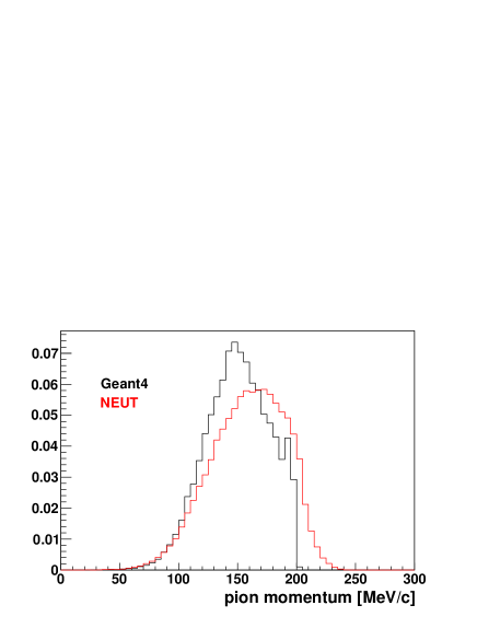
Figure 28: Predicted momentum distribution of pions from inelastic scattering event, for Geant4 (black) and NEUT (red), for $p_{\pi}=$ 201.6 MeV/c. The histograms are normalized by area.

V.1.10 Summary of the systematic errors

As summarized in Table 5, the total error is $\sim$6.5%, except for $p_{\pi}=216.6$ MeV/c data set, which is roughly half of the errors of the previous experimentsAshery et al. (1981); Navon et al. (1983, 1979). For $p_{\pi}=$ 216.6 MeV/c data set, the statistical error is relatively large, and the systematic error is also found to be large.

V.2 Result

Table 7 summarizes the measurements for five momentum data sets. The errors in $\sigma_{\mathrm{ABS}+\mathrm{CX}}$ includes both statistical and systematic uncertainties.

$p_{\pi}$	$N_{\mathrm{data}}$	$N_{\mathrm{BG}}^{pred}$	$N_{\mathrm{sig}}^{pred}$	$R_{\mathrm{TiO}}^{data}$	$R_{\mathrm{TiO}}^{\mathrm{MC}}$	$f_{\mu}$	$\sigma_{\mathrm{ABS}+\mathrm{CX}}^{pred}$	$\sigma_{\mathrm{ABS}+\mathrm{CX}}$
[MeV/c]							[mbarn]	[mbarn]
201.6	6797	1708.9	4622.3	0.0634	0.0808	0.0016	175.93	197.9${}^{+10.9}_{-15.3}$
216.6	1814	452.3	1243.6	0.0636	0.0731	0.0071	194.41	215.8${}^{+17.3}_{-18.6}$
237.2	7671	2047.0	5572.0	0.0624	0.0632	0.0043	214.43	216.6${}^{+12.0}_{-13.3}$
265.5	6772	1851.4	5153.7	0.0603	0.0528	0.0054	235.92	224.8${}^{+14.8}_{-14.2}$
295.1	7266	1745.4	5745.8	0.0591	0.0518	0.0034	219.39	211.4${}^{+14.1}_{-12.9}$

Table 7: Summary of the measurements. In this table, $p_{\pi}$ is the momentum of pions at the fiber tracker.

Figure 29 shows the measured $\sigma_{\mathrm{ABS}+\mathrm{CX}}$ as a function of pion momentum, compared with the results from previous experimentsAshery et al. (1981); Navon et al. (1983).

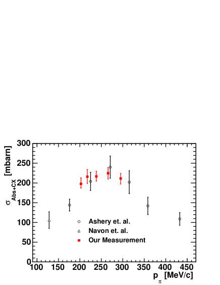
Figure 29: Result of $\sigma_{\mathrm{ABS}+\mathrm{CX}}$ vs. Pion momentum, compared with the results from previous experiments.

As already mentioned, the uncertainty in our measurement is roughly half of the uncertainty in the previous experiments. In these experiments $\sigma_{\mathrm{ABS}+\mathrm{CX}}$ was measured by subtracting the pion scattering cross-section from the total cross-section. Since the ABS and CX events were not selected directly there were large errors (typically 5 $\sim$ 10% in Ashery et al. (1981)) assigned for the subtraction procedure. In our measurements, thanks to a fine-grained fully active fiber tracker, we were able to measure the ABS + CX interaction directly.

To summarize, we obtained the cross section for ABS + CX of positive pions in carbon nuclei at an incident momentum between 201.6 MeV/c to 295.1 MeV/c. The uncertainty of our measurement is smaller than previous experiments by nearly half due to the newly developed fully active scintillation fiber tracker. This result will be a important input to existing models such as Geant4 or NEUT to constrain low momentum pion interactions.