Poisson-Fermi Model of Single Ion Activities

Abstract

A Poisson-Fermi model is proposed for calculating activity coefficients of single ions in strong electrolyte solutions based on the experimental Born radii and hydration shells of ions in aqueous solutions. The steric effect of water molecules and interstitial voids in the first and second hydration shells play an important role in our model. The screening and polarization effects of water are also included in the model that can thus describe spatial variations of dielectric permittivity, water density, void volume, and ionic concentration. The activity coefficients obtained by the Poisson-Fermi model with only one adjustable parameter are shown to agree with experimental data, which vary nonmonotonically with salt concentrations.

1 Introduction

Comprehensive discussions of theoretical and experimental studies on the activity coefficient of single ions in electrolyte solutions have been recently given by Fraenkel [1], Valikó and Boda [2], and Rowland et al. [3], where more references can also be found. The Poisson-Fermi (PF) model proposed in this paper belongs to the continuum approach that traces back to the simple, elegant, but very coarse theory — the Debye-Hückel (DH) theory. As mentioned by Fraenkel, the continuum theory has evolved in the past century into a series of modified Poisson-Boltzmann (PB) equations that can involve an overwhelmingly large number of parameters in order to fit Monte Carlo (MC), molecular dynamics (MD), or experimental data. Many expressions of those parameters are rather long and tedious and do not have clear physical meaning [1].

The Debye-Hückel model is derived from a linearized PB equation [4]. Extended from the DH model, the Pitzer model [5] is the most eminent approach to modeling the thermodynamic properties of multicomponent electrolyte solutions due to its unmatched precision over wide ranges of temperature and pressure [3]. However, the combinatorial explosion of adjustable parameters in the extended DH modeling functions (including Pitzer) can cause profound difficulties in fitting experimental data and independent verification because the parameters are very sensitive to numerous related thermodynamic properties in multicomponent systems [3]. The Poisson-Fermi model proposed here involves only one adjustable parameter.

The ineffectiveness of previous Poisson-Boltzmann models is mainly due to inaccurate treatments of the steric and correlation effects of ions and water molecules whose nonuniform charges and sizes can have significant impact on the activities of all particles in an electrolyte system. Unfortunately, the point charge particles of PB theories have electric fields that are most approximate where they are largest, near the point. PB theories are not an appealing choice for the leading terms in a series of approximations, for that reason. The PF theory developed in our papers [6, 7, 8, 9, 10] demonstrates how these two effects can be described by a simple steric potential and a correlation length of ions. The parameters of the PF theory describe distinct physical properties of the system in a clear way [9]. The Gibbs-Fermi free energy of the PF model reduces to the classical Gibbs free energy of the PB model when the steric potential and correlation length are omitted [9]. The PF model has been verified with either MC, MD or double layer data at (more or less) equilibrium [6, 7, 8], and nonequilibrium data from calcium and gramicidin channels [9, 10].

Here, we apply the PF theory to study the activity properties of individual ions in strong electrolytes. The steric effect of all particles and the interstitial voids that accompany them are described by a Fermi-like distribution that defines the water densities in the hydration shell of a solvated ion and the particle concentrations in the solvent region outside the hydration shell. The resulting correlations produce a dielectric function that shows variations in permittivity around the solvated ion. The experimental concentration-dependent dielectric constant model proposed in [2] is used to define the concentration-dependent Born radii of the solvated ion in the present work. The experimental data of the activity coefficients of NaCl and CaCl₂ electrolytes reported in [11] are used to test the PF model.

2 Theory

The activity coefficient $\gamma_{i}$ of an ion of species $i$ in electrolyte solutions describes the deviation of the chemical potential of the ion from ideality ($\gamma_{i}=1$). The excess chemical potential is $\mu_{i}^{\text{ex}}=k_{B}T\ln\gamma_{i}$, where $k_{B}$ is the Boltzmann constant and $T$ is an absolute temperature. In Poisson-Boltzmann theory, the excess chemical potential can be calculated by [12]

$$\mu_{i}^{\text{ex}}=\Delta G_{i}^{\text{PB}}-\Delta G_{i}^{0}\text{, \ }\Delta G_{i}^{\text{PB}}=\frac{1}{2}q_{i}\phi^{\text{PB}}(\mathbf{0})\text{, \ }\Delta G_{i}^{0}=\frac{1}{2}q_{i}\phi^{0}(\mathbf{0})\text{,}$$ (1)

where the center of the hydrated ion (also denoted by $i$) is set to the origin $\mathbf{0}$ for convenience in the following discussion and $q_{i}$ is the ionic charge. The potential function $\phi^{\text{PB}}(\mathbf{r})$ of spatial variable $\mathbf{r}$ is found by solving the Poisson-Boltzmann equation

$$-\epsilon_{s}\nabla^{2}\phi^{\text{PB}}(\mathbf{r}) =\sum_{j=1}^{K}q_{j}C_{j}(\mathbf{r})=\rho(\mathbf{r})\text{,}$$ (2)

$$C_{j}(\mathbf{r}) =C_{j}^{\text{B}}\exp\left(-\beta_{j}\phi^{\text{PB}}(\mathbf{r})\right)\text{,}$$ (3)

where the concentration function $C_{j}(\mathbf{r})$ is described by a Boltzmann distribution (3) with a constant bulk concentration $C_{j}^{\text{B}}$, $\epsilon_{s}=\epsilon_{\text{w}}\epsilon_{0}$, $\epsilon_{\text{w}}$ is the dielectric constant of bulk water, and $\epsilon_{0}$ is the vacuum permittivity. The potential $\phi^{0}(\mathbf{r})$ of the ideal system is obtained by setting $\rho(\mathbf{r})=0$ in (2), i.e., all ions of $K$ species in the system do not electrostatically interact with each other since $q_{j}=0$ for all $j$. We consider a large domain $\Omega$ of the system in which $\phi^{\text{PB}}(\mathbf{r})=0$ on the boundary of the domain $\partial\Omega$. The ideal potential $\phi^{0}(\mathbf{r})$ is then a constant, i.e., $\Delta G_{i}^{0}$ is a constant reference chemical potential independent of $C_{j}^{\text{B}}$.

For an equivalent binary system, the Debye-Hückel theory simplifies the calculation by analytically solving a linearized equation of (2) so that the potential function $\phi^{\text{PB}}(\mathbf{r})$ becomes a constant [4]

$$\phi^{\text{DH}}=-\frac{q_{i}\kappa}{4\pi\epsilon_{s}}\text{, \ }\frac{1}{\kappa}=\left(\frac{\epsilon_{s}k_{B}T}{\sum_{j=1}^{2}q_{j}^{2}C_{j}^{\text{B}}L}\right)^{1/2}$$ (4)

dependent of the bulk concentration $C_{j}^{\text{B}}$, where $L$ is the Avogadro constant.

The Poisson-Fermi equation proposed in [9] is

$$\epsilon_{s}\left(l_{c}^{2}\nabla^{2}-1\right)\nabla^{2}\phi^{\text{PF}}(\mathbf{r})=\sum_{j=1}^{K+1}q_{j}C_{j}(\mathbf{r})=\rho(\mathbf{r})\text{, }\forall\mathbf{r}\in\Omega_{s}$$ (5)

$$C_{j}(\mathbf{r})=C_{j}^{\text{B}}\exp\left(-\beta_{j}\phi^{\text{PF}}(\mathbf{r})+S^{\text{trc}}(\mathbf{r})\right)\text{, \ \ }S^{\text{trc}}(\mathbf{r})=\ln\frac{\Gamma(\mathbf{r)}}{\Gamma^{\text{B}}}\text{,}$$ (6)

where $S^{\text{trc}}(\mathbf{r})$ is called the steric potential, $\Gamma(\mathbf{r)}=1-\sum_{j=1}^{K+1}v_{j}C_{j}(\mathbf{r})$ is a void fraction function, $\Gamma^{\text{B}}=1-\sum_{j=1}^{K+1}v_{j}C_{j}^{\text{B}}$ is a constant void fraction, and $v_{j}$ is the volume of a species $j$ particle (hard sphere). Note that the PF equation includes water as the last species of particles with the zero charge $q_{K+1}=0$. The polarization of the water and solution is an output of the theory. The water can be described more realistically, for example, as a quadrupole in later versions of the theory. The distribution (6) is of Fermi type since all concentration functions are bounded above, i.e., $C_{j}(\mathbf{r})<1/v_{j}$ for all particle species with any arbitrary (or even infinite) potential $\phi(\mathbf{r})$ at any location $\mathbf{r}$ in the domain $\Omega$ [9]. The Boltzmann distribution (3) would however diverge if $\phi(\mathbf{r})$ tends to infinity. This is a major deficiency of PB theory for modeling a system with strong local electric fields or interactions. The PF equation (5) and the Fermi distribution reduce to the PB equation (2) and the Boltzmann distribution (3), respectively, when $l_{c}=S^{\text{trc}}=0$, i.e., when the correlation and steric effects are not considered.

If the correlation length $l_{c}=2a_{i}\neq 0$, the dielectric operator $\widehat{\epsilon}=\epsilon_{s}(1-l_{c}^{2}\nabla^{2})$ approximates the permittivity of the bulk solvent and the linear response of correlated ions [6, 7, 13, 14], where $a_{i}$ is the radius of the ion. The dielectric function $\widetilde{\epsilon}(\mathbf{r})=\epsilon_{s}/(1+\eta/\rho)$ is a further approximation of $\widehat{\epsilon}$. It is found by transforming (5) into two second-order PDEs [6]

$$\epsilon_{s}\left(l_{c}^{2}\nabla^{2}-1\right)\Psi(\mathbf{r}) =\rho(\mathbf{r})$$ (7)

$$\nabla^{2}\phi^{\text{PF}}(\mathbf{r}) =\Psi(\mathbf{r})$$ (8)

by introducing a density like variable $\Psi$ that yields a polarization charge density $\eta=-\epsilon_{s}\Psi-\rho$ of water using Maxwell’s first equation [7]. Boundary conditions of the new variable $\Psi$ on the boundary $\partial\Omega$ were derived from the global charge neutrality condition [6].

To obtain more accurate potentials at the origin $\mathbf{0}$, i.e., $\phi^{\text{PF}}(\mathbf{0})$, we need to consider the size and hydration shell of the hydrated ion $i$. The domain $\Omega$ is partitioned into three parts such that $\Omega=$ $\overline{\Omega}_{\text{Ion}}\cup\overline{\Omega}_{\text{Sh}}\cup\Omega_{\text{Solv}}$, where $\Omega_{\text{Ion}}$ is the spherical domain occupied by the ion $i$, $\Omega_{\text{Sh}}$ is the hydration shell of the ion, and $\Omega_{\text{Solv}}$ is the rest of the solvent domain as shown in Fig. 1. The radii of $\Omega_{\text{Ion}}$ and the outer boundary of $\Omega_{\text{Sh}}$ are denoted by $R_{i}^{Born}$ and $R_{i}^{Sh}$, respectively, whose values will be determined by experimental data. It is natural to choose the Born radius $R_{i}^{Born}$ as the radius of $\Omega_{\text{Ion}}$ [12]. We consider both first and second shells of the ion [15, 16]. The dielectric constants in $\overline{\Omega}_{\text{Ion}}$ and $\Omega\backslash\overline{\Omega}_{\text{Ion}}$ are denoted by $\epsilon_{\text{ion}}$ and $\epsilon_{\text{w}}$, respectively.

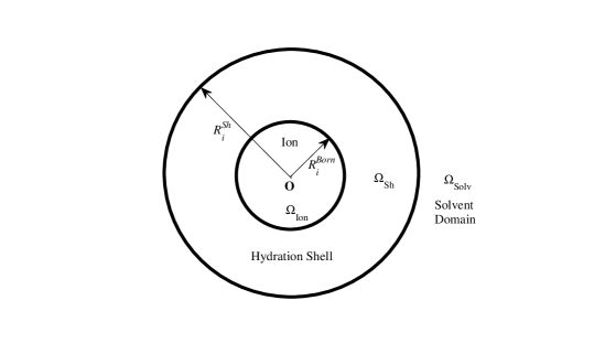
Figure 1: The model domain $\Omega$ is partitioned into the ion domain $\Omega_{\text{Ion}}$ (with radius $R_{i}^{Born}$), shell domain $\Omega_{\text{Sh}}$ (with radius $R_{i}^{Sh}$), and solvent domain $\Omega_{\text{Solv}}$.

The PF equation (5) then becomes

$$\epsilon\left(l_{c}^{2}\nabla^{2}-1\right)\nabla^{2}\phi^{\text{PF}}(\mathbf{r})=\rho(\mathbf{r})=\left\{\begin{array}[c]{l}q_{i}\delta(\mathbf{r}-\mathbf{0})\text{ in }\overline{\Omega}_{\text{Ion}}\\ \sum_{j=1}^{K+1}q_{j}C_{j}(\mathbf{r})\text{ in }\Omega\backslash\overline{\Omega}_{\text{Ion}},\end{array}\right.$$ (9)

where $\delta(\mathbf{r}-\mathbf{0})$ is the delta function at the origin, $l_{c}=0$ in $\overline{\Omega}_{\text{Ion}}$, $l_{c}\neq 0$ in $\Omega\backslash\overline{\Omega}_{\text{Ion}}$, $\epsilon=\epsilon_{\text{ion}}\epsilon_{0}$ in $\overline{\Omega}_{\text{Ion}}$, and $\epsilon=\epsilon_{s}=\epsilon_{\text{w}}\epsilon_{0}$ in $\Omega\backslash\overline{\Omega}_{\text{Ion}}$. The shell radius $R_{i}^{Sh}$ is determined by Eq. (6) as

$$S_{\text{Sh}}^{\text{trc}}=\ln\frac{V_{\text{Sh}}-v_{\text{w}}O_{i}^{\text{w}}}{V_{\text{Sh}}\Gamma^{\text{B}}}=\ln\frac{O_{i}^{\text{w}}}{V_{\text{Sh}}C_{\text{w}}^{\text{B}}}\Rightarrow V_{\text{Sh}}=\frac{\Gamma^{\text{B}}}{C_{\text{w}}^{\text{B}}}O_{i}^{\text{w}}+v_{\text{w}}O_{i}^{\text{w}}\text{,}$$ (10)

where $v_{\text{w}}$ is the volume of a water molecule and $V_{\text{Sh}}$ is the volume of the hydration shell that depends on the bulk void fraction $\Gamma^{\text{B}}$, the bulk water density $C_{\text{w}}^{\text{B}}$, and the total number $O_{i}^{\text{w}}$ (coordination number) of water molecules occupying the shell of the hydrated ion $i$. Note that the shell volume $V_{\text{Sh}}$ varies with bulk ionic concentrations $C_{j}^{\text{B}}$. The occupancy number $O_{i}^{\text{w}}$ is given by experimental data [15, 16] and so is the shell volume that of course determines the shell radius $R_{i}^{Sh}$.

To deal with the singular problem of the delta function $\delta(\mathbf{r}-\mathbf{0})$ in Eq. (9), we use the numerical methods proposed in [6] to calculate $\phi^{\text{PF}}(\mathbf{r})$ as follows:

(i)

Solve the Laplace equation $\nabla^{2}\phi^{\text{L}}(\mathbf{r})=0$ in $\Omega_{\text{Ion}}$ with the boundary condition $\phi^{\text{L}}(\mathbf{r})=\phi^{\ast}(\mathbf{r})=q_{i}/(4\pi\epsilon_{\text{ion}}\epsilon_{0}\left|\mathbf{r-0}\right|)$ on $\partial\Omega_{\text{Ion}}$.

(ii)

Solve the Poisson-Fermi equation (9) in $\Omega\backslash\overline{\Omega}_{\text{Ion}}$ with the jump condition $\left[\epsilon\nabla\phi^{\text{PF}}(\mathbf{r})\cdot\mathbf{n}\right]=-\epsilon_{\text{ion}}\epsilon_{0}\nabla(\phi^{\ast}(\mathbf{r})+\phi^{\text{L}}(\mathbf{r}))\cdot\mathbf{n}$ on $\partial\Omega_{\text{Ion}}$ and the zero boundary condition $\phi^{\text{PF}}(\mathbf{r})=0$ on $\partial\Omega$, where $\left[u\right]$ denotes the jump function across $\partial\Omega_{\text{Ion}}$ [6].

The evaluation of the Green function $\phi^{\ast}(\mathbf{r})$ on $\partial\Omega_{\text{Ion}}$ always yields finite numbers and thus avoids the singularity. Note that our model can be applied to electrolyte solutions at any temperature $T$ having any arbitrary number ($K$) of ionic species with different size spheres and valences.

3 Results

Numerical values of model notations are given in Table 1, where the occupancy number $O_{i}^{\text{w}}=18$ is taken to be the experimental coordination number of the calcium ion Ca²⁺ given in [15] for all ions $i=$ Na⁺, Ca²⁺, and Cl^- since the electric potential produced by the solvated ion diminishes exponentially in the outer shell region in which a small variation of $O_{i}^{\text{w}}$ for $i=$ Na⁺ and Cl^- does not affect numerical approximations too much. Obviously the coordination number may be different for different types of ions and at different concentrations and so on. We were surprised that we can fit experimental data so well using a single experimentally determined occupancy number for all ions and conditions.

As discussed in [2], the solvation free energy of an ion $i$ should vary with salt concentrations and can be expressed by a dielectric constant $\epsilon(C_{i}^{\text{B}})$ that depends on the bulk concentration of the ion $C_{i}^{\text{B}}$. Following [2], we assume that

$$\epsilon(C_{i}^{\text{B}})=\epsilon_{\text{w}}-\delta_{i}C_{i}^{\text{B}}+\left(C_{i}^{\text{B}}\right)^{3/2}$$ (11)

with only one parameter $\delta_{i}$, whose value is given in Table 1, instead of two in [2]. Note that $\epsilon(C_{i}^{\text{B}})$ is a constant when the dimensionless $C_{i}^{\text{B}}$ is given. It is not a function of a spatial variable $\mathbf{r}$ like $\widetilde{\epsilon}(\mathbf{r})$. The parameter $\delta_{i}$ represents the ratio of the factor of $C_{i}^{\text{B}}$ to that of $\left(C_{i}^{\text{B}}\right)^{3/2}$ in the original formula, where the factors of various electrolytes are taken from various sources of either theoretical or experimental data [2]. Our ratios $\delta_{i}$ in Table 1 are comparable with those given in [2].

The Born formula of the solvation energy can thus be modified as

$$\Delta G_{i}^{\text{Born}}(C_{i}^{\text{B}})=\frac{q_{i}^{2}}{8\pi\epsilon_{0}\theta(C_{i}^{\text{B}})R_{i}^{0}}\left(\frac{1}{\epsilon_{\text{w}}}-1\right)\text{, \ \ }\theta(C_{i}^{\text{B}})=\frac{\epsilon(C_{i}^{\text{B}})\left(\epsilon_{\text{w}}-1\right)}{\epsilon_{\text{w}}\left(\epsilon(C_{i}^{\text{B}})-1\right)},$$ (12)

where $R_{i}^{0}$ is the Born radius when $C_{i}^{\text{B}}=0$ ($\theta(0)=1$) and $R_{i}^{Born}=\theta(C_{i}^{\text{B}})R_{i}^{0}$ is the concentration-dependent Born radius used to define $\Omega_{\text{Ion}}$ in Fig. 1 when $C_{i}^{\text{B}}\neq 0$. The Born radii $R_{i}^{0}$ in Table 1 are cited from [2], which are computed from the experimental hydration Helmholtz free energies of these ions given in [17]. All values in Table 1 are either physical or experimental data except that of $\delta_{i}$, which is the only adjustable parameter in our model. All these values were kept fixed throughout calculations.

Table 1. Values of Model Notations Symbol Meaning  Value  Unit $k_{B}$ Boltzmann constant $1.38\times 10^{-23}$ J/K $T$ temperature $298.15$ K $e$ proton charge $1.602\times 10^{-19}$ C $\epsilon_{0}$ permittivity of vacuum $8.85\times 10^{-14}$ F/cm $\epsilon_{\text{ion}}$, $\epsilon_{\text{w}}$ dielectric constants $1$, $78.45$ $l_{c}=2a_{i}$ correlation length $i=\text{Na}^{+}$,$\text{Ca}^{2+}$, $\text{Cl}^{-}$ Å $a_{\text{Na}^{+}}$, $a_{\text{Ca}^{2+}}$ radii $0.95$, $0.99$ Å $a_{\text{Cl}^{-}}$, $a_{\text{H}_{2}\text{O}}$ radii $1.81$, $1.4$ Å $R_{\text{Na}^{+}}^{0},$ $R_{\text{Ca}^{2+}}^{0}$, $R_{\text{Cl}^{-}}^{0}$ Born radii in Eq. (12) $1.617$, $1.706$, $2.263$ Å $\delta_{\text{Na}^{+}}$, $\delta_{\text{Ca}^{2+}}$, $\delta_{\text{Cl}^{-}}$ in Eq. (11) 4.2, 5.1, 3.8 $O_{i}^{\text{w}}$ in Eq. (10) 18   

The PF results of Na⁺, Ca²⁺, and Cl^- activity coefficients agree well with the experimental data [11] as shown in Figs. 2 and 3 for NaCl and CaCl₂ electrolytes, respectively, with various [NaCl] and [CaCl₂] from 0 to 2.5 M. In Fig. 4, we observe that the Debye-Hückel theory oversimplifies the Ca²⁺ activity coefficient to a straight line as frequently mentioned in physical chemistry texts [4] because the theory does not account for the steric and correlation effects of ions and water, let alone the atomic structure of the ion and its hydration shell as shown in Fig. 1. Both PB and PF results in Fig. 4 were obtained using the same atomic Fermi formula (10) for shell radii $R_{i}^{Sh}$ in $\overline{\Omega}_{\text{Sh}}$ and the same concentration-dependent Born formula (12) for Born radii $R_{i}^{Born}$ in $\overline{\Omega}_{\text{Ion}}$. Therefore, the only difference between PB and PF is in $\Omega_{\text{Solv}}$, where $l_{c}=S^{\text{trc}}=0$ for PB and $l_{c}\neq 0$ and $S^{\text{trc}}\neq 0$ for PF. Note that these two formulas are not present in previous PB models. Fig. 4 shows that the correlation and steric effects still play a significant role in the solvent domain $\Omega_{\text{Solv}}$ although the domain is $R_{\text{Ca}^{2+}}^{Sh}=4.95$ Å (not shown) away from the center of the Ca²⁺ ion. The ion and shell domains are the most crucial region to study ionic activities. For example, Fraenkel’s theory is entirely based on this region — the so-called smaller-ion shell region [1].

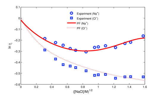
Figure 2: Comparison of PF results with experimental data [11] on $i=$ Na⁺ and Cl^- activity coefficients $\gamma_{i}$ in various [NaCl] from 0 to 2.5 M.

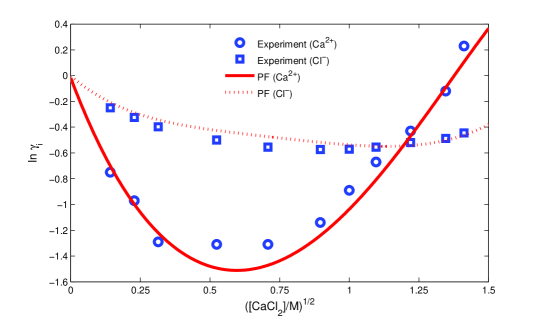
Figure 3: Comparison of PF results with experimental data [11] on $i=$ Ca²⁺ and Cl^- activity coefficients $\gamma_{i}$ in various [CaCl₂] from 0 to 2 M.

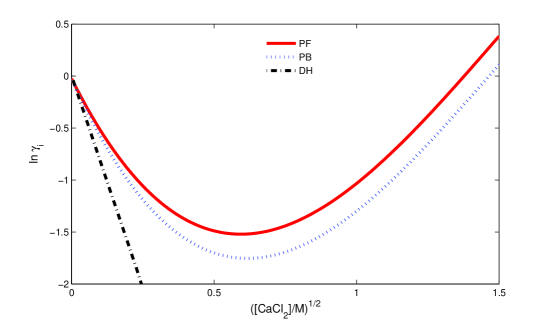
Figure 4: Comparison of Poisson-Fermi (PF), Poisson-Boltzmann (PB), and Debye-Hückel (DH) results on $i=$ Ca²⁺ activity coefficients $\gamma_{i}$ in various [CaCl₂] from 0 to 2 M.

The PF model can provide more physical details near the solvated ion (Ca²⁺, for example) in a strong electrolyte ([CaCl₂] = 2 M) such as the dielectric function $\widetilde{\epsilon}(\mathbf{r})$ of varying permittivity (shown in Fig. 5), variable water density $C_{\text{H}_{\text{2}}\text{O}}(\mathbf{r})$ (in Fig. 5), concentration of counterion ($C_{\text{Cl}^{-}}(\mathbf{r})$ in Fig. 6), electric potential ($\phi^{\text{PF}}(\mathbf{r})$ in Fig. 6), and the steric potential ($S^{\text{trc}}(\mathbf{r})$ in Fig. 6). Note that the dielectric function $\widetilde{\epsilon}(\mathbf{r})$ is an output, not an input of the model. The steric effect is small because the configuration of particles (voids between particles) does not vary too much from the solvated region to the bulk region. However, the variation of mean-field water densities $C_{\text{H}_{\text{2}}\text{O}}(\mathbf{r})$ has a significant effect on the dielectrics in the hydration region as shown by the dielectric function $\widetilde{\epsilon}(\mathbf{r})$. The strong electric potential $\phi^{\text{PF}}(\mathbf{r})$ in the Born cavity $\overline{\Omega}_{\text{Ion}}$ and the water density $C_{\text{H}_{\text{2}}\text{O}}(\mathbf{r})$ in the hydration shell $\Omega_{\text{Sh}}$ are the most important factors leading the PF results to match the experimental data. PF theory deals well with the much more concentrated solutions in ion channels where void effects are important [9].

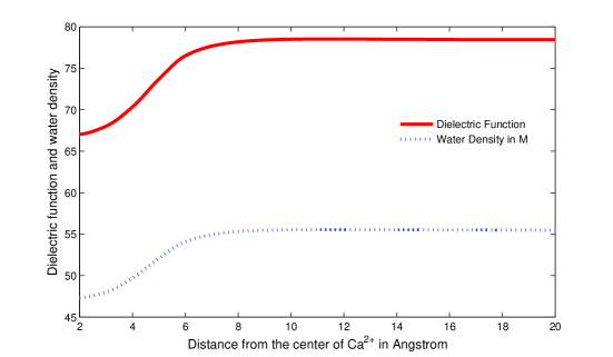
Figure 5: Dielectric $\widetilde{\epsilon}(\mathbf{r})$ and water density $C_{\text{H}_{\text{2}}\text{O}}(\mathbf{r})$ profiles near the solvated ion Ca²⁺ with [CaCl₂] $=2$ M.

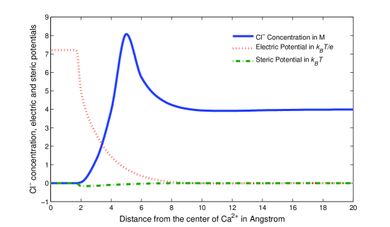
Figure 6: Cl^- concentration $C_{\text{Cl}^{-}}(\mathbf{r})$, electric potential $\phi^{\text{PF}}(\mathbf{r})$, and steric potential $S^{\text{trc}}(\mathbf{r})$ profiles near the solvated ion Ca²⁺ with [CaCl₂] $=2$ M.

4 Conclusion

We have proposed a Poisson-Fermi model for studying activities of single ions in strong electrolyte solutions. The atomic structure of ionic cavity and hydration shells of a solvated ion is modeled by the Born theory and Fermi distribution using experimental data. The steric effect of ions and water of nonuniform sizes with interstitial voids and the correlation effect of ions are also considered in the model. With only one adjustable parameter in the model, it is shown that the atomic structure and these two effects play a crucial role to match experimental activity coefficients that vary nonmonotonically with salt concentrations.

5 Acknowledgements

This work was supported in part by the Ministry of Science and Technology of Taiwan under Grant No. 103-2115-M-134-004-MY2 to J.L.L.

References

- [1] D. Fraenkel, Simplified electrostatic model for the thermodynamic excess potentials of binary strong electrolyte solutions with size-dissimilar ions, Mol. Phys. 108, 1435 (2010).
- [2] M. Valiskó, D. Boda, Unraveling the behavior of the individual ionic activity coefficients on the basis of the balance of ion-ion and ion-water interactions, J. Phys. Chem. B 119, 1546 (2015).
- [3] D. Rowland, E. Königsberger, G. Hefter, and P. M. May, Aqueous electrolyte solution modelling: Some limitations of the Pitzer equations, Appl. Geochem. 55, 170 (2015).
- [4] K. J. Laidler, J. H. Meiser, and B. C. Sanctuary, Physical Chemistry (Houghton Mifflin Co., Boston, 2003).
- [5] K. S. Pitzer, Thermodynamics of electrolytes. I. Theoretical basis and general equations, J. Phys. Chem. 77, 268 (1973).
- [6] J.-L. Liu, Numerical methods for the Poisson-Fermi equation in electrolytes, J. Comp. Phys. 247, 88 (2013).
- [7] J.-L. Liu and B. Eisenberg, Correlated ions in a calcium channel model: a Poisson-Fermi theory, J. Phys. Chem. B 117, 12051 (2013).
- [8] J.-L. Liu and B. Eisenberg, Analytical models of calcium binding in a calcium channel, J. Chem. Phys. 141, 075102 (2014).
- [9] J.-L. Liu and B. Eisenberg, Poisson-Nernst-Planck-Fermi theory for modeling biological ion channels, J. Chem. Phys. 141, 22D532 (2014).
- [10] J.-L. Liu and B. Eisenberg, Numerical methods for a Poisson-Nernst-Planck-Fermi model of biological ion channels, to appear in Phys. Rev. E (2015).
- [11] G. Wilczek-Vera, E. Rodil, and J. H. Vera, On the activity of ions and the junction potential: Revised values for all data, AIChE. J. 50, 445 (2004).
- [12] D. Bashford and D. A. Case, Generalized Born models of macromolecular solvation effects, Annu. Rev. Phys. Chem. 51, 129 (2000).
- [13] C. D. Santangelo, Computing counterion densities at intermediate coupling, Phys. Rev. E 73, 041512 (2006).
- [14] M. Z. Bazant, B. D. Storey, and A. A. Kornyshev, Double layer in ionic liquids: Overscreening versus crowding, Phys. Rev. Lett. 106, 046102 (2011).
- [15] W. W. Rudolph and G. Irmer, Hydration of the calcium(II) ion in an aqueous solution of common anions (ClO, Cl-, Br-, and NO), Dalton Trans. 42, 3919 (2013).
- [16] J. Mähler and I. Persson, A study of the hydration of the alkali metal ions in aqueous solution, Inorg. Chem. 51, 425 (2011).
- [17] W. R. Fawcett, Liquids, Solutions, and Interfaces: From Classical Macroscopic Descriptions to Modern Microscopic Details (Oxford University Press, New York, 2004).