Density profiles, dynamics, and condensation in the ZRP conditioned on an atypical current

Abstract

We study the asymmetric zero-range process (ZRP) with $L$ sites and open boundaries, conditioned to carry an atypical current. Using a generalized Doob $h$-transform we compute explicitly the transition rates of an effective process for which the conditioned dynamics are typical. This effective process is a zero-range process with renormalized hopping rates, which are space dependent even when the original rates are constant. This leads to non-trivial density profiles in the steady state of the conditioned dynamics, and, under generic conditions on the jump rates of the unconditioned ZRP, to an intriguing supercritical bulk region where condensates can grow. These results provide a microscopic perspective on macroscopic fluctuation theory (MFT) for the weakly asymmetric case: It turns out that the predictions of MFT remain valid in the non-rigorous limit of finite asymmetry. In addition, the microscopic results yield the correct scaling factor for the asymmetry that MFT cannot predict.

Keywords: Zero-range processes, Large deviations in non-equilibrium systems, Stochastic particle dynamics (Theory)

1 Introduction

There has been considerable progress in recent years in the understanding of nonequilibrium, current-carrying systems [1, 2, 3, 4, 5]. Recently, much effort has been devoted to the study of fluctuations which result in atypical currents in such systems [1, 5], where equilibrium concepts of entropy and free energy could be generalized to a nonequilibrium setting. Following the seminal papers [6, 7], the non-typical large-deviation behaviour of Markovian stochastic lattice gas models has come under intense scrutiny in the framework of what is now known as macroscopic fluctuation theory (MFT) [5]. In particular, the asymmetric simple exclusion process (ASEP) [8, 9] has been studied in great detail under the condition that the dynamics exhibits a strongly atypical current for a very long interval of time. Among the questions of considerable importance is the optimal density profile that realizes such a rare large deviation. Using MFT it was found for the weakly asymmetric simple exclusion process, where the hopping bias is of order $1/L$, that for an atypically low current a dynamical phase transition occurs in the case of periodic boundary conditions: Above a critical non-typical current the optimal macroscopic density profile is flat, while rare events below that critical current are typically realized by a traveling wave [10]. This phenomenon was subsequently been studied numerically with Monte-Carlo simulations [11, 12]. Non-flat optimal profiles were obtained also for open boundary conditions [13].

More recently, the space-time realizations of large-deviation events in the ASEP with finite (strong) hopping bias were studied on the microscopic scale. This was done by conditioning the time-integrated current in a finite time interval to attain some atypical value. Furthermore, the full conditioned probability distribution on a finite lattice has been examined. For low non-typical current, the microscopic structure of a fluctuating traveling wave and an antishock has been identified [14, 15, 16]. Recently duality was used to extend the microscopic approach to show that the traveling wave may exhibit a microscopic fine structure consisting of several shocks and antishocks [17]. These findings are consistent with the macroscopic results for the optimal density profile [10, 13], but provide much more information in that the complete time-dependent measure was obtained for the microscopic dynamics.

Using a type of Doob’s $h$-transform [18, 19, 20, 21] one may also study the large time limit on microscopic lattice scale. This transformation generates effective dynamics which make the rare large deviation behaviour of the original dynamics typical. For the ASEP with periodic boundary conditions and large non-typical current, inaccessible to MFT, it was found that a different dynamical phase transition involving a change of dynamical universality class occurs: Instead of the well-known generic universality class of the KPZ equation with dynamical exponent $z=3/2$ for the typical dynamics [22] one has a ballistic universality class with dynamical exponent $z=1$ where fluctuations spread much faster [23, 24, 25]. In fact, it turns out that these results follow predictions from conformal field theory and are thus expected to be universal [26]. Moreover, using the $h$-transform technique, long-range effective interactions which make these rare events typical were obtained [23].

In this paper, we study similar questions, regarding the emergence of atypical currents, in another prototypical model of nonequilibrium systems — the zero range process (ZRP) [27, 28]. The steady state of the ZRP is exactly soluble, and thus it has often been used in studies of out-of-equilibirum features. The ZRP is a stochastic lattice gas model where each lattice site $i$ can be occupied by an arbitrary number $n_{i}\geq 0$ of particles. Particles move randomly to neighbouring sites with a rate $u(n_{i})$ that depends only on the occupation number of the departure site and not on the state of the rest of the lattice. We consider a one-dimensional lattice of sites $i=1,\ldots,L$ with open boundaries where the system exchanges particles with external reservoirs. The hopping events may be biased in one direction.

The precise definition of the model is given below. As an introduction we summarize some well-known features of the ZRP. The stationary state of the model with periodic boundary conditions, where the total particle number is conserved, may exhibit a condensation transition above a critical density. In this scenario, the existence of which depends on the form of the hopping rates $u(n)$, all sites but one are occupied by a particle number that fluctuates around the critical density, while one randomly selected site carries all the remaining excess particles, whose number is of the order of the lattice size (for a review see [28]). On the other hand, for open boundary conditions where the total particle number fluctuates due to random injection and absorption of particles at the two boundaries of the system, the scenario is different: For boundary rates for which a stationary distribution exists condensation never occurs. Only in the non-stationary case of very strong injection a dynamical condensation phenomenon occurs: The boundary sites can become supercritical, in which case the occupation number of these sites grows indefinitely [29]. This gives rise to a non-stationary condensate-like structure, but, in further contrast to the usual stationary bulk condensate, this can happen for any choice of bounded hopping rates $u(n)$ and, moreover, the phenomenon is strictly limited to the boundary sites.

This brief outline of the properties of the ZRP concerns typical behaviour of the stochastic dynamics. It is the purpose of this work to study on microscopic scale the behaviour of the ZRP in a regime of strongly atypical behaviour of the particle current. This is of interest for several reasons. First, it serves not only as a test for macroscopic fluctuation theory (MFT) [5], but also probes its validity in the regime of strong asymmetry where MFT is not rigorous. Second, we will be able to compute effective microscopic interactions that make atypical behaviour typical. Third, it will transpire that unexpected and novel condensation patterns can occur even when the unconditioned dynamics do not exhibit condensation.

Current large deviations of finite duration have been investigated for the ZRP in the context of the breakdown of the Gallavotti-Cohen symmetry for the current distribution in a ZRP with open boundary conditions [30, 31]. It turns out that the failure of the Gallavotti-Cohen symmetry argument, which is based on a very general time-reversal property of stochastic dynamics [32, 33], can be related to the formation of “instantaneous condensates” [30]. These condensates were investigated recently in terms of Doob’s $h$-transform for the ZRP with a single site [34]. It was shown that in some parameter regimes, Doob’s $h$-transform fails to represent the effective dynamics that make the large deviation typical.

The microscopic large-deviation properties of the ZRP in the regime of atypical currents that persist for a very long time have not yet been explored. In this paper we address this problem. Moreover, we do not limit ourselves a single site; rather, we consider the full problem of open boundaries with any number of sites. It turns out that Doob’s $h$-transform can be computed exactly from a product ansatz for the lowest eigenvector. Thus we are able to calculate the effective interactions that make the current large deviations typical. This turns out to be a ZRP with space-dependent hopping bias. Interestingly, the effective process satisfies detailed balance if and only of one conditions on vanishing macroscopic current. These results are outside the scope of MFT.

Somewhat surprisingly the exact results show that bulk condensation in the conditioned open system may occur, as is the case for periodic boundary conditions under typical dynamics. However, in contrast to typical behaviour (and to naive expectation), the results suggest that a whole lattice segment may become supercritical rather than just a single site. The segment location and length are fixed by the current on which one conditions rather than randomly fluctuating as one has for the condensate position in the periodic case with typical dynamics.

Our exact results are valid for any asymmetry, including the weakly asymmetric case. This allows for a comparison with the predictions of the macroscopic fluctuation theory which we apply to the ZRP with weak asymmetry. The microscopic results show that the MFT results remain intact in the limit of finite asymmetry, a limit in which the validity of the macroscopic approach is a-priori questionable. Moreover, we obtain the scaling factor for the asymmetry that cannot be computed from the MFT.

The paper is organized as follows: In Sec. 2 we introduce the model and define the conditioned dynamics. In Sec. 3 we derive the exact microscopic results for the $h$-transform. This yields the effective dynamics and the spatial condensation patterns of the conditioned process. In Sec. 4 we follow the macroscopic approach for the weakly asymmetric case to compute the optimal macroscopic profile that realizes a current large deviation.

2 Open ZRP conditioned on an atypical current

2.1 Definition of the model

In the bulk of the lattice a particle from site $i$ hops to site $i+1$ with rate $pu(n_{i})$, and to site $i-1$ with rate $qu(n_{i})$. The parameters $p$ and $q$ determine the asymmetry of the process: The hopping is symmetric when $p=q$ and asymmetric otherwise. For the function $u(n)$ we have $u(0)=0$, as particles cannot leave an empty site, otherwise $u(n)>0$ is arbitrary. By definition the $i$th bond is between sites $i$ and $i+1$ for $1\leq i\leq L-1$. Bond 0 ($L$) represents the link between the lattice and a left (right) boundary reservoir that is not modeled explicitly. At the left boundary, particles enter with rate $\alpha$ from the left reservoir and exit with rate $\gamma u(n_{1})$. Similarly, at the right boundary particles enter with rate $\delta$ from the right boundary reservoir and exit with rate $\beta u(n_{L})$ (Fig. 1).

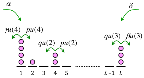
Figure 1: Some possible particle hopping events in the ZRP with $L$ sites and open boundary conditions.

The dynamics of the zero-range process can be conveniently represented using the quantum Hamiltonian formalism [9, 35]. In this approach one defines a probability vector $|P\rangle=\sum_{\mathbf{n}}P_{\mathbf{n}}\mbox{$|\,{\mathbf{n}}\,\rangle$}$ where $\mbox{$|\,{\mathbf{n}}\,\rangle$}=|n_{1})\otimes\dots\otimes|n_{L})$ is the canonical basis vector of $(\mathbb{C}^{\infty})^{\otimes L}$ associated with the particle configuration $\mathbf{n}=(n_{1},n_{2},\ldots,n_{L})$ and $P_{\mathbf{n}}$ the probability measure on the set of all such configurations. For a single site in this tensor product the configuration with $n$ particles on that site is represented by the basis vector $|n)$ which has component 1 at position $n+1$ and zero elsewhere. By definition $|P\rangle$ obeys the normalization condition $\langle\mathbf{S}|P\rangle=1$ with the summation vector

$$\mbox{$\langle\,{\mathbf{S}}\,|$}=\sum_{\mathbf{n}}\mbox{$\langle\,{\mathbf{n}}\,|$}$$ (1)

and the orthogonality condition $\langle\mathbf{n}|\mathbf{n}^{\prime}\rangle=\delta_{\mathbf{n},\mathbf{n}^{\prime}}$. Within this formalism the Markovian time evolution of the ZRP is represented by the Master equation

$$\frac{\rmd}{\rmd t}|P(t)\rangle=-\hat{H}|P(t)\rangle$$ (2)

with

$$\hat{H} = \hat{h}_{0}+\sum_{k=1}^{L-1}\hat{h}_{k}+\hat{h}_{L}$$ (3)

$$= -\biggl{\{}\sum_{k=1}^{L-1}\left[p(\hat{a}_{k}^{-}\hat{a}^{+}_{k+1}-\hat{d}_{k})+q(\hat{a}_{k}^{+}\hat{a}_{k+1}^{-}-\hat{d}_{k+1})\right]$$

$$+\alpha(\hat{a}_{1}^{+}-1)+\gamma(\hat{a}_{1}^{-}-\hat{d}_{1})+\delta(\hat{a}_{L}^{+}-1)+\beta(\hat{a}^{-}_{L}-\hat{d}_{L})\biggr{\}}$$

where $\hat{a}^{+}$ and $\hat{a}^{-}$ are infinite-dimensional particle creation and annihilation matrices

$$\hat{a}^{+}=\left(\begin{array}[]{ccccc}0&0&0&0&\ldots\\ 1&0&0&0&\ldots\\ 0&1&0&0&\ldots\\ 0&0&1&0&\ldots\\ \ldots&\ldots&\ldots&\ldots&\ldots\end{array}\right),\qquad\hat{a}^{-}=\left(\begin{array}[]{ccccc}0&u(1)&0&0&\ldots\\ 0&0&u(2)&0&\ldots\\ 0&0&0&u(3)&\ldots\\ 0&0&0&0&\ldots\\ \ldots&\ldots&\ldots&\ldots&\ldots\end{array}\right)$$ (4)

and $\hat{d}=\sum u(r)|r)(r|$ is a diagonal matrix with the $(r,s)$th element given by $u(r)\delta_{r,s}$. The subscript $k$ in $\hat{a}^{\pm}_{k}$ and $\hat{d}_{k}$ indicates that the respective matrix acts non-trivially on site $k$ of the lattice and as unit operator on all other sites. We also introduce the local particle number operator $\hat{n}_{k}$ with the diagonal particle number matrix $\hat{n}=\sum r|r)(r|$ and note the useful identity

$$y^{\hat{n}}\hat{a}^{\pm}y^{-\hat{n}}=y^{\pm 1}\hat{a}^{\pm}$$ (5)

for any non-zero complex number $y$. The global particle number operator $\hat{N}=\sum_{k=1}^{L}\hat{n}_{k}$ commutes with the bulk part of $\hat{H}$, expressing particle number conservation of the bulk jump processes.

According to (2) the probability vector at time $t$ is given by

$$\mbox{$|\,{P(t)}\,\rangle$}=\exp{(-\hat{H}t)}\mbox{$|\,{P(t)}\,\rangle$}.$$ (6)

Using $(s|\hat{a}^{+}=(s|$ and $(s|\hat{a}^{-}=(s|\hat{d}$ for the one-site summation vector $(s|=\sum_{n}(n|$ one verifies that the global summation vector (1) is a left eigenvector of $\hat{H}$ with zero eigenvalue. This expresses conservation of probability through the relation $0=d/(dt)\mbox{$\langle\,{\mathbf{S}}\,|\,{P(t)}\,\rangle$}=-\mbox{$\langle\,{\mathbf{S}}\,|$}\hat{H}\mbox{$|\,{P(t)}\,\rangle$}$. A stationary distribution, denoted $|\,{P^{\ast}}\,\rangle$, is a right eigenvector of $\hat{H}$ with eigenvalue zero.

In [29] it is shown that the stationary distribution of the ZRP is given by a product measure

$$|P^{*}\rangle=|P^{*}_{1})\otimes|P^{*}_{2})\otimes\ldots\otimes|P^{*}_{L})$$ (7)

where the marginal distribution $|P^{*}_{k})$ is the single-site probability vector with components

$$P^{*}_{k}:=\mbox{${\rm Prob}\left[\,{n_{k}=n}\,\right]$}=\frac{z_{k}^{n}}{Z_{k}}\prod_{i=1}^{n}u(i)^{-1}.$$ (8)

The empty product is defined to be equal to 1 and $Z_{k}$ is the local partition function

$$Z_{k}\equiv Z(z_{k})=\sum_{n=0}^{\infty}z_{k}^{n}\prod_{i=1}^{n}u(i)^{-1}.$$ (9)

The fugacities $z_{k}$ in the steady state are given by

$$z_{k}=\frac{[(\alpha+\delta)(p-q)-\alpha\beta+\gamma\delta]\left(\frac{p}{q}\right)^{k-1}-\gamma\delta+\alpha\beta\left(\frac{p}{q}\right)^{L-1}}{\gamma(p-q-\beta)+\beta(p-q+\gamma)\left(\frac{p}{q}\right)^{L-1}}.$$ (10)

The mean density at site $k$ is related to the fugacity by (see (8)–(9))

$$\rho_{k}=\langle n_{k}\rangle=\frac{d\log Z_{k}}{d\log z_{k}}$$ (11)

The absence of detailed balance is reflected in a steady-state current

$$j^{\ast}=(p-q)\frac{-\gamma\delta+\alpha\beta\left(\frac{p}{q}\right)^{L-1}}{\gamma(p-q-\beta)+\beta(p-q+\gamma)\left(\frac{p}{q}\right)^{L-1}}.$$ (12)

Notice that the existence of a steady state is determined by the radius of convergence of $Z_{k}$. If the form of the transition rates results in some $z_{k}$ outside this radius of convergence, then a stationary distribution does not exist. One expects relaxation to the local marginal distribution wherever the radius of convergence is finite, and a growing condensate on the other sites [29].

2.2 Grandcanonical conditioning

By ergodicity, the stationary current $j^{\ast}$ is the long-time mean of the time-integrated current $J_{k}(t)$ across a bond $k,k+1$, i.e. of the number of positive particle jumps from site $k$ to $k+1$ minus the number of negative particle jumps from site $k+1$ to $k$ up to time $t$. Because of bulk particle number conservation the stationary current does not depend on $k$. It is of great interest to consider not only the mean $j^{\ast}$, but also the fluctuations of the time-averaged current $j_{k}(t)=J_{k}(t)/t$, in particular its large deviations. The distribution $g_{k}(j,t):=\mbox{${\rm Prob}\left[\,{j_{k}(t)=j}\,\right]$}$ has the large deviation property $g_{k}(j,t)\propto\rme^{-F_{k}(j)t}$ [33]. For particle systems with finite state space the large deviation function does not depend on the site $k$ and satisfies the Gallavotti-Cohen symmetry [32, 33] and this is widely believed to be generic. However, it has been pointed out that neither statement remains valid for the ZRP with open boundaries if one considers sufficiently large atypical currents. In order to get deeper insight into this breakdown we study here the ZRP conditioned to produce a strong atypical current. However, instead on enforcing a particular (integer) value of the time-integrated current, we consider a “grandcanonical” conditioning defined in terms of a Legrende transform with conjugate parameter $s$. This corresponds to an ensemble of ZRP-histories where the current is allowed to fluctuate around some atypical mean. We refer to this ensemble as the $s$-ensemble.

Grandcanonically conditioned Markov processes may be studied in the spirit of Doob’s $h$-transform [18, 19], as was done for the ASEP conditioned on very large currents in [14, 23, 24], see also [20, 21] for recent discussions. This microscopic approach also provides a construction to compute effective interactions for which the atypical behaviour becomes typical, see [14, 23] for applications to the ASEP. Besides the conceptual insight gained in this way into extreme behaviour, this is potentially interesting from a practical perspective: By adjusting interactions between particles, one obtains a means to make desirable, but normally rare, events frequent.

Following [36, 37] this construction is done by first defining a weighted generator $\hat{H}(s)$ where the operators that correspond to a jump to the right (left) are multiplied by a factor $\rme^{s}$ ($\rme^{-s}$). Then one considers the lowest left eigenvector of $\hat{H}(s)$, i.e., the eigenvector $\langle\,{0}\,|$ to the lowest eigenvalue of $\hat{H}(s)$, which we denote by $\epsilon_{0}(s)$. We also introduce the diagonal matrix $\hat{D}(s)$ which has the components $D_{\mathbf{n}}(s)$ of the lowest eigenvector on its diagonal. Since all off-diagonal elements of $\hat{H}(s)$ are non-positive we appeal to Perron-Frobenius theory and argue that all components of $\langle\,{0}\,|$ can be chosen to be real and non-zero. Thus $\hat{D}$ is invertible and we have

$$\mbox{$\langle\,{0}\,|$}=\mbox{$\langle\,{\mathbf{S}}\,|$}\hat{D}(s),\quad\mbox{$\langle\,{0}\,|$}\hat{D}^{-1}(s)=\mbox{$\langle\,{\mathbf{S}}\,|$}.$$ (13)

This allows us to introduce the grandcanonical Doob’s $h$-transform

$$\hat{G}(s)=\hat{D}(s)\hat{H}(s)\hat{D}^{-1}(s)-\epsilon_{0}(s).$$ (14)

Notice that by construction $\hat{G}(s)$ has non-positive off-diagonal elements and, moreover, by (13), $\mbox{$\langle\,{\mathbf{S}}\,|$}\hat{G}(s)=0$. Hence $\hat{G}(s)$ is the generator of some Markov process, which we shall refer to as the effective generator, with jump rates $\tilde{w}_{\mathbf{n}^{\prime},\mathbf{n}}(s)=w_{\mathbf{n}^{\prime},\mathbf{n}}D_{\mathbf{n}^{\prime}}(s)D^{-1}_{\mathbf{n}}(s)$. We denote by $P^{\ast}_{\mathbf{n}}(s)$ the invariant measure of the effective process $\hat{G}(s)$. The steady state of this Markov process provides the steady state of the grandcanonically biased $s$ model. It is easy to prove that $P^{\ast}_{\mathbf{n}}(s)=D_{\mathbf{n}}(s)\Gamma_{\mathbf{n}}(s)$ where $\Gamma_{\mathbf{n}}(s)$ are the components of the lowest right eigenvector of the weighted generator $\hat{H}(s)$. In order to avoid heavy notation we suppress in the following the dependence on $s$ if there is no danger of confusion.

2.3 Local conditioning in the ZRP

Under the condition that the mean integrated current across some fixed bond $(k,k+1)$ fluctuates around a certain value parameterized by $s$ we obtain, following Ref. [37], the weighted generator

$$\hat{H}^{(k)}(s)=\sum_{l=0}^{k-1}\hat{h}_{l}+\hat{h}_{k}(s)+\sum_{l=k+1}^{L}\hat{h}_{l}.$$ (15)

Here

$$\hat{h}_{0}(s) = -\left[\alpha(\rme^{s}\hat{a}_{1}^{+}-1)+\gamma(\rme^{-s}\hat{a}_{1}^{-}-\hat{d}_{1})\right]$$

$$\hat{h}_{k}(s) = -\left[p(\rme^{s}\hat{a}_{k}^{-}\hat{a}^{+}_{k+1}-\hat{d}_{k})+q(\rme^{-s}\hat{a}_{k}^{+}\hat{a}_{k+1}^{-}-\hat{d}_{k+1})\right],\quad 1\leq k\leq L-1$$

$$\hat{h}_{L}(s) = -\left[\delta(\rme^{-s}\hat{a}_{L}^{+}-1)+\beta(\rme^{s}\hat{a}^{-}_{L}-\hat{d}_{L})\right].$$ (16)

We refer to this setting as local conditioning. Notice that $\hat{h}_{k}(0)=\hat{h}_{k}$. We denote the lowest left eigenvector of $\hat{H}^{(k)}$ by $\mbox{$\langle\,{Y_{k}}\,|$}=\mbox{$\langle\,{\mathbf{S}}\,|$}\hat{D}_{k}$. Specifically for $k=0$ we drop the subscript $0$ i.e., we write $\mbox{$\langle\,{Y_{0}}\,|$}=\mbox{$\langle\,{Y}\,|$}=\mbox{$\langle\,{\mathbf{S}}\,|$}\hat{D}$

Define the partial number operator $\hat{N}_{k}=\sum_{i=1}^{k}\hat{n}_{i}$. From (5) one concludes $\hat{H}^{(k)}(s)=\rme^{-s\hat{N}_{k}}\hat{H}^{(0)}(s)\rme^{s\hat{N}_{k}}$. This implies for the left eigenvector

$$\mbox{$\langle\,{Y_{k}}\,|$}\hat{H}^{(k)}(s)=\mbox{$\langle\,{Y_{k}}\,|$}\epsilon_{0}$$ (17)

where the lowest eigenvalue is independent of $k$ and

$$\mbox{$\langle\,{Y_{k}}\,|$}=\mbox{$\langle\,{Y}\,|$}\rme^{s\hat{N}_{k}}=\mbox{$\langle\,{\mathbf{S}}\,|$}\hat{D}_{k}$$ (18)

with $\hat{D}_{k}=\hat{D}\rme^{s\hat{N}_{k}}$. This yields effective dynamics

$$\hat{G}^{(k)}(s)=\hat{D}_{k}\hat{H}^{(k)}(s)\hat{D}_{k}^{-1}-\epsilon_{0}=\hat{D}\hat{H}^{(0)}(s)\hat{D}^{-1}-\epsilon_{0}=\hat{G}^{(0)}(s).$$ (19)

We conclude that the effective dynamics does not depend on $k$ and we can focus on conditioning on a current across bond $0$, i.e. between the left reservoir and site 1 of the lattice.

3 Microscopic density profiles and condensation

3.1 Left eigenvector

The left eigenvector of $\hat{H}^{(0)}(s)$ was computed in [30]. For self-containedness we repeat here the essential steps, which are based on a product ansatz $\mbox{$\langle\,{Y}\,|$}=(y_{1}|\otimes(y_{2}|\otimes\ldots\otimes(y_{L}|=\mbox{$\langle\,{\mathbf{S}}\,|$}\hat{D}$ with the diagonal matrix $\hat{D}=y_{1}^{n}\otimes\ldots y_{L}^{n}$ where $n$ are the diagonal one-site number operators. Then

$$-\mbox{$\langle\,{Y}\,|$}\hat{H}^{(0)}(s) = \mbox{$\langle\,{Y}\,|$}\left\{\alpha(y_{1}\rme^{s}-1)+\gamma(\rme^{-s}-y_{1})\hat{d}_{1}y_{1}^{-1}+\right.$$

$$\sum_{k=1}^{L-1}\left[p(y_{k+1}-y_{k})\hat{d}_{k}y_{k}^{-1}+q(y_{k}-y_{k+1})\hat{d}_{k+1}y_{k+1}^{-1}\right]+$$

$$\left.\delta(y_{L}-1)+\beta(1-y_{L})\hat{d}_{L}y_{L}^{-1}\right\}$$

$$= \mbox{$\langle\,{Y}\,|$}\left\{\alpha(y_{1}\rme^{s}-1)+\left[\gamma(\rme^{-s}-y_{1})+p(y_{2}-y_{1})\right]\hat{d}_{1}y_{1}^{-1}+\right.$$

$$\sum_{k=2}^{L-1}\left[p(y_{k+1}-y_{k})+q(y_{k-1}-y_{k})\right]\hat{d}_{k}y_{k}^{-1}+$$

$$\left.\delta(y_{L}-1)+\left[q(y_{L-1}-y_{L})+\beta(1-y_{L})\right]\hat{d}_{L}y_{L}^{-1}\right\}.$$

One sees that $\langle\,{Y}\,|$ is a left eigenvector if the following equations are satisfied:

$$0 = p(y_{k+1}-y_{k})+q(y_{k-1}-y_{k})$$ (22)

$$0 = \gamma(\rme^{-s}-y_{1})+p(y_{2}-y_{1})$$ (23)

$$0 = q(y_{L-1}-y_{L})+\beta(1-y_{L}).$$ (24)

We define the hopping asymmetry $a=p/q$. The ansatz

$$y_{k}=A+Ba^{L+1-k}$$ (25)

yields $y_{k-1}-y_{k}=B(a-1)a^{L+1-k}$ and therefore solves (22).

The left boundary equation (23) yields

$$\rme^{-s}-A-Ba^{L}+pBa^{L}(a^{-1}-1)/\gamma=0$$ (26)

which gives

$$A=\rme^{-s}-(p-q+\gamma)\frac{Ba^{L}}{\gamma}.$$ (27)

On the other hand, the right boundary equation (24) yields

$$B(p-q)a+\beta(1-A-Ba)=0$$ (28)

Plugging this into $A$ leads to

$$B=\frac{\beta\gamma(\rme^{-s}-1)a^{-1}}{\gamma(p-q-\beta)+\beta(p-q+\gamma)a^{L-1}}$$ (29)

and

$$A=\frac{\gamma\rme^{-s}(p-q-\beta)+\beta(p-q+\gamma)a^{L-1}}{\gamma(p-q-\beta)+\beta(p-q+\gamma)a^{L-1}}=1+\frac{\gamma(\rme^{-s}-1)(p-q-\beta)}{\gamma(p-q-\beta)+\beta(p-q+\gamma)a^{L-1}}.$$ (30)

For the lowest eigenvalue we get

$$\epsilon_{0} = -(\alpha(y_{1}\rme^{s}-1)+\delta(y_{L}-1))$$

$$= \frac{\alpha}{\gamma}p\rme^{s}(y_{1}-y_{2})-\frac{\delta}{\beta}q(y_{L-1}-y_{L})$$

$$= (p-q)(\frac{\alpha}{\gamma}a^{-1}\rme^{s}-\frac{\delta}{\beta}a^{-L})Ba^{L+1}$$

from which one finds

$$\epsilon_{0}=(p-q)(\rme^{-s}-1)\frac{\alpha\beta a^{L-1}\rme^{s}-\gamma\delta}{\gamma(p-q-\beta)+\beta(p-q+\gamma)a^{L-1}}.$$ (32)

3.2 Right eigenvector

Following [30] we make a product ansatz also for the right eigenvector: $\mbox{$|\,{X}\,\rangle$}=|x_{1})\otimes|x_{2})\otimes\ldots\otimes|x_{L})$ where $|x_{k})$ is the unnormalized vector with components

$$(Q^{*}_{k})_{n}=x_{k}^{n}\prod_{i=1}^{n}u(i)^{-1}.$$ (33)

This yields

$$-\hat{h}_{k}\mbox{$|\,{X}\,\rangle$} = (px_{k}-qx_{k+1})\left(\frac{\hat{d}_{k}}{x_{k}}-\frac{\hat{d}_{k+1}}{x_{k+1}}\right)\mbox{$|\,{X}\,\rangle$}$$ (34)

$$-\hat{h}_{0}(s)\mbox{$|\,{X}\,\rangle$} = (\alpha\rme^{s}-\gamma x_{1})\left(\rme^{-s}-\frac{\hat{d}_{1}}{x_{1}}\right)\mbox{$|\,{X}\,\rangle$}$$ (35)

$$-\hat{h}_{L}\mbox{$|\,{X}\,\rangle$} = (\beta x_{L}-\delta)\left(1-\frac{\hat{d}_{L}}{x_{L}}\right)\mbox{$|\,{X}\,\rangle$}$$ (36)

One sees that $|\,{X}\,\rangle$ is a right eigenvector if the following equations are satisfied:

$$b = px_{k}-qx_{k+1}$$ (37)

$$b = \alpha\rme^{s}-\gamma x_{1}$$ (38)

$$b = \beta x_{L}-\delta$$ (39)

with some constant $b$. The ansatz

$$x_{k}=C+Da^{k}$$ (40)

yields $px_{k}-qx_{k+1}=C(p-q)$ and therefore solves (22) with $b=C(p-q)$. Using the boundary recursions one then obtains

$$C=\frac{\alpha\beta\rme^{s}a^{L-1}-\gamma\delta}{\beta(p-q+\gamma)a^{L-1}+\gamma(p-q-\beta)}$$ (41)

and

$$D=a^{-1}\frac{\alpha\rme^{s}(p-q-\beta)+\delta(p-q+\gamma)}{\beta(p-q+\gamma)a^{L-1}+\gamma(p-q-\beta)}.$$ (42)

Notice that in terms of the local fugacities $x_{k}$ one has

$$\epsilon_{0}=-\alpha+\gamma\rme^{-s}x_{1}-\delta+\beta x_{L}=C(1-\rme^{-s}).$$ (43)

3.3 Effective dynamics

The transformation (5) yields for the bulk hopping terms

$$-\hat{D}\hat{h}_{k}\hat{D}^{-1} = p\left(\frac{y_{k+1}}{y_{k}}\hat{a}_{k}^{-}\hat{a}_{k+1}^{+}-\hat{d}_{k}\right)+q\left(\frac{y_{k}}{y_{k+1}}\hat{a}_{k}^{+}\hat{a}_{k+1}^{-}-\hat{d}_{k+1}\right)$$

$$= p\frac{y_{k+1}}{y_{k}}\left(\hat{a}_{k}^{-}\hat{a}_{k+1}^{+}-\hat{d}_{k}\right)+q\frac{y_{k}}{y_{k+1}}\left(\hat{a}_{k}^{+}\hat{a}_{k+1}^{-}-\hat{d}_{k+1}\right)$$

$$+(p-q)\left(1-\frac{A}{y_{k+1}}\right)\hat{d}_{k+1}-(p-q)\left(1-\frac{A}{y_{k+1}}\right)\hat{d}_{k}$$

and for the boundaries

$$-\hat{D}\hat{h}_{0}\hat{D}^{-1} = \alpha(y_{1}\rme^{s}\hat{a}_{1}^{+}-1)+\gamma(y_{1}^{-1}\rme^{-s}\hat{a}_{1}^{-}-\hat{d}_{1})$$

$$= \alpha y_{1}\rme^{s}(\hat{a}_{1}^{+}-1)+\gamma y_{1}^{-1}\rme^{-s}(\hat{a}_{1}^{-}-\hat{d}_{1})$$

$$+\alpha(y_{1}\rme^{s}-1)+(p-q)y_{1}^{-1}(y_{1}-A)\hat{d}_{1}$$

and

$$-\hat{D}\hat{h}_{L}\hat{D}^{-1} = \delta(y_{L}\hat{a}_{L}^{+}-1)+\beta(y_{L}^{-1}\hat{a}^{-}_{L}-\hat{d}_{L})$$

$$= \delta y_{L}(\hat{a}_{L}^{+}-1)+\beta y_{L}^{-1}(\hat{a}^{-}_{L}-\hat{d}_{L})$$

$$+\delta(y_{L}-1)+(p-q)y_{L}^{-1}(y_{L}-A)\hat{d}_{L}$$

Therefore the effective dynamics is given by

$$\hat{G}^{(0)}(s) = \hat{D}\hat{G}^{(0)}\hat{D}^{-1}-\epsilon_{0}$$

$$= -\sum_{k=1}^{L-1}\left[p\frac{y_{k+1}}{y_{k}}\left(\hat{a}_{k}^{-}\hat{a}_{k+1}^{+}-\hat{d}_{k}\right)+q\frac{y_{k}}{y_{k+1}}\left(\hat{a}_{k}^{+}\hat{a}_{k+1}^{-}-\hat{d}_{k+1}\right)\right]$$

$$-\left[\alpha y_{1}\rme^{s}(\hat{a}_{1}^{+}-1)+\gamma y_{1}^{-1}\rme^{-s}(\hat{a}_{1}^{-}-\hat{d}_{1})\right]$$

$$-\left[\delta y_{L}(\hat{a}_{L}^{+}-1)+\beta y_{L}^{-1}(\hat{a}^{-}_{L}-\hat{d}_{L})\right]$$

It is intriguing that this is a driven ZRP with a spatially varying driving field $E_{k}(s)=\log{a}+2\log{y_{k+1}(s)/y_{k}(s)}$. This space-dependence will be present even in the case of non-interacting particles with $u(n)=wn$. Therefore, conditioning on an atypical local current can be realized by an effective process with a space-dependent driving field.

The stationary distribution of the effective dynamics is a product state

$$\mbox{$|\,{P^{*}(s)}\,\rangle$}=|P^{*}_{1}(s))\otimes|P^{*}_{2}(s))\otimes\ldots\otimes|P^{*}_{L}(s))$$ (48)

where $|P^{*}_{k}(s))$ is the probability vector with components

$$(P^{*}_{k}(s))_{n}=\frac{z_{k}^{n}}{Z_{k}}\prod_{i=1}^{n}u(i)^{-1}.$$ (49)

Here

$$z_{k}=x_{k}y_{k}$$ (50)

is the local fugacity given by (25) together with (29), (30) and (40) together with (41) (42). The normalization $Z_{k}$ is the local analogue of the grand-canonical partition function, given by (9) as before. The density at site $k$ is related to the fugacity as in the unconditioned ZRP by Eq. (11). For example, for non-interacting particles $u(n)=n$, and therefore the density is simply $\rho_{k}=z_{k}$. It is remarkable that one obtains a non-trivial density profile even for non-interacting particles.

The stationary current is

$$j^{\ast}(s)=px_{k}y_{k+1}-qy_{k}x_{k+1}=\alpha y_{1}\rme^{s}-\gamma x_{1}\rme^{-s}=\beta x_{L}-\delta y_{L}=(p-q)(AC-BDa^{L+1}).$$ (51)

Plugging in the expressions yields

$$j^{\ast}(s)=(p-q)\frac{\alpha\beta\rme^{s}a^{L-1}-\gamma\delta\rme^{-s}}{\beta(p-q+\gamma)a^{L-1}+\gamma(p-q-\beta)}.$$ (52)

3.4 Examples

We now explore in more depth the results of the previous subsections for some specific choices of the model parameters.

3.4.1 Barrier-free reservoirs

To somewhat reduce the parameter space of the model, it is natural to consider

$$\beta = p$$ (53)

$$\gamma = q,$$ (54)

i.e., the hopping rates out of the first and last site are the same as the bulk hopping rates. We further simplify the notation by reexpressing the parameters $\alpha$ and $\delta$ in terms of reservoir fugacities:

$$\alpha = z_{l}\,\gamma\,p/q=z_{l}\,p$$ (55)

$$\delta = z_{r}\,\beta\,q/p=z_{r}\,q$$ (56)

where $z_{l}$ is the fugacity of the left reservoir and $z_{r}$ is that of the right reservoir. The interpretation is that in the original (unconditioned) process, particles jump with the same rate between reservoir and boundary sites as inside the bulk of the chain. We therefore refer to this choice of rates as “barrier-free reservoirs”.

A few further notations will prove useful in what follows. First, we express the hopping asymmetry $a=p/q$ via

$$\tilde{\nu}=\frac{L+1}{2}\log a.$$ (57)

It is further convenient to characterize the boundary reservoirs by chemical potentials $z_{i}=\rme^{\mu_{i}}$, and to define parameters $\Delta\mu$, $\bar{\mu}$ and $z_{0}$ as follows

$$\Delta\mu \equiv \mu_{l}-\mu_{r}=\log(z_{l}/z_{r}),$$ (58)

$$\bar{\mu} \equiv (\mu_{l}+\mu_{r})/2,$$ (59)

$$z_{0} \equiv \rme^{\bar{\mu}}=\sqrt{z_{l}z_{r}}.$$ (60)

Finally, we define a relative position along the lattice

$$r_{k}=\frac{k}{L+1}.$$ (61)

3.4.2 Partially asymmetric ZRP with barrier-free reservoirs

With the choice (53)–(56) the parameters $A,B,C,D$ take the simpler form

$$A=\frac{a^{L+1}-\rme^{-s}}{a^{L+1}-1} B=\frac{\rme^{-s}-1}{a^{L+1}-1}$$ (62)

$$C=\frac{z_{l}\rme^{s}a^{L+1}-z_{r}}{a^{L+1}-1} D=\frac{z_{r}-z_{l}\rme^{s}}{a^{L+1}-1}.$$ (63)

This leads to

$$y_{k}=1-(1-\rme^{-s})\frac{a^{L+1-k}-1}{a^{L+1}-1}=\frac{\rme^{\tilde{\nu}(1-r_{k})}\sinh[\tilde{\nu}r_{k}]+\rme^{-s-\tilde{\nu}r_{k}}\sinh[\tilde{\nu}(1-r_{k})]}{\sinh[\tilde{\nu}]}.$$ (64)

The effective hopping rates can now be read off Eq. (3.3). They corresponds to a ZRP in which the bulk bias to jump to the left and right is site dependent: a particle hops from site $k$ to $k+1$ with rate $u(n_{k})p_{k}$ and from site $k$ to $k-1$ with rate $u(n_{k})q_{k}$ where

$$p_{k}=p\frac{y_{k+1}}{y_{k}}=\sqrt{pq}\,\frac{\rme^{s+\tilde{\nu}}\sinh[\tilde{\nu}r_{k+1}]+\sinh[\tilde{\nu}(1-r_{k+1})]}{\rme^{s+\tilde{\nu}}\sinh[\tilde{\nu}r_{k}]+\sinh[\tilde{\nu}(1-r_{k})]}$$ (65)

and

$$q_{k}=q\frac{y_{k-1}}{y_{k}}=\sqrt{pq}\,\frac{\rme^{s+\tilde{\nu}}\sinh[\tilde{\nu}r_{k-1}]+\sinh[\tilde{\nu}(1-r_{k-1})]}{\rme^{s+\tilde{\nu}}\sinh[\tilde{\nu}r_{k}]+\sinh[\tilde{\nu}(1-r_{k})]}.$$ (66)

These rates correspond to a space-dependent local field

$$E_{k}=\log\frac{p_{k}}{q_{k+1}}=2\log\frac{\rme^{s+\tilde{\nu}}\sinh[\tilde{\nu}r_{k+1}]+\sinh[\tilde{\nu}(1-r_{k+1})]}{\rme^{s+\tilde{\nu}}\sinh[\tilde{\nu}r_{k}]+\sinh[\tilde{\nu}(1-r_{k})]}.$$ (67)

It is interesting to note that the effective bulk hopping rates, and thus the effective field, are independent of the reservoir fugacities.

At the left boundary (site 1), according to (3.3), particles are effectively injected with rate $z_{l}\,p_{0}$ and removed with rate $q_{1}$, where $p_{0},q_{1}$ are given in (65) and (66). Similarly at the right boundary (site $L$) the effective injection and removal rates are $z_{r}\,q_{L+1}$ and $p_{L}$, respectively. Thus, the effective boundary dynamics remains of the barrier-free form with the same reservoir fugacities, and only the effective space-dependent hopping rates depend on the current-conditioning.

We proceed to examine the typical fugacity profile during the atypical current event. To this end, we first calculate the right eigenvector

$$x_{k}=\frac{z_{l}\rme^{s}a^{L+1}+(z_{r}-z_{l}\rme^{s})a^{k}-z_{r}}{a^{L+1}-1}=\frac{z_{l}\rme^{s+\tilde{\nu}r_{k}}\sinh[\tilde{\nu}(1-r_{k})]+z_{r}\rme^{-\tilde{\nu}(1-r_{k})}\sinh[\tilde{\nu}r_{k}]}{\sinh[\tilde{\nu}]}.$$ (68)

Thus, the fugacity profile $z_{k}=x_{k}y_{k}$ is

$$z_{k}=z_{0}\frac{\rme^{\frac{\Delta\mu}{2}}\sinh^{2}[\tilde{\nu}(1-r_{k})]+\rme^{-\frac{\Delta\mu}{2}}\sinh^{2}[\tilde{\nu}r_{k}]+2\tilde{Q}\sinh[\tilde{\nu}r_{k}]\sinh[\tilde{\nu}(1-r_{k})]}{\sinh^{2}\tilde{\nu}},$$ (69)

with

$$\tilde{Q}=\cosh\Bigl{(}s+\frac{\Delta\mu}{2}+\tilde{\nu}\Bigr{)}.$$ (70)

The fugacity profile (69) along with the effective driving field are plotted in figure 2 for strongly asymmetric dynamics, and in figure 3 for weakly asymmetric dynamics.

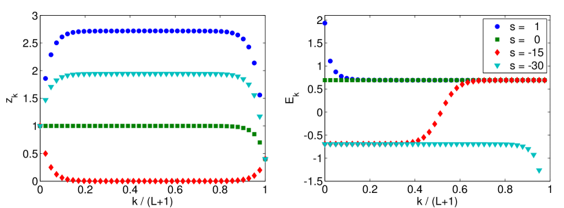
Figure 2: The fugacity profile $z_{k}$ (left) and the effective field $E_{k}$ (right) for an asymmetric ZRP with $p=1$, $q=1/2$, $z_{l}=1$, $z_{r}=0.4$, and $L=40$. Several values of $s$ are plotted including the typical profile of the unconditioned process ($s=0$). The fugacity profile and the effective field are both flat, except for boundary layers of size $O(1)$ sites.

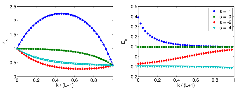
Figure 3: The fugacity profile $z_{k}$ (left) and the effective field $E_{k}$ (right) for a weakly-asymmetric ZRP with $p=1/2+2/L$, $q=1/2$, $z_{l}=1$, $z_{r}=0.4$, and $L=40$. Several values of $s$ are plotted including the typical profile of the unconditioned process ($s=0$). The solid lines correspond to the macroscopic result, Eqs. (109) and (123).

The current is

$$j^{\ast}(s)=(p-q)\frac{z_{l}\rme^{s}a^{L+1}-z_{r}\rme^{-s}}{a^{L+1}-1}=2\sqrt{pq}\,\frac{\sinh(\frac{\tilde{\nu}}{L+1})\sinh\bigl{(}\tilde{\nu}+s+\frac{\Delta\mu}{2}\bigr{)}}{\sinh(\tilde{\nu})}.$$ (71)

This current could be generated by a ZRP with the same constant bulk hopping rates $p,q$ as in the original (unconditioned) dynamics but with effective reservoir fugacities $z_{l}^{\mathrm{eff}}=z_{l}\rme^{s}$ and $z_{r}^{{\mathrm{eff}}}=z_{r}\rme^{-s}$. However, as pointed out above, in a finite system this is not how the conditioned process is typically realized. There is a space-dependent driving field and the effective fugacities $z_{k}$ are not those of an effective left reservoir with boundary fugacity $z_{l}\rme^{s}$.

3.4.3 Symmetric ZRP

For $p=q$ both $A$ and $B$ of Eqs. (29) and (30) diverge, but $y_{k}$ is well-defined. One gets

$$y_{k}=1+\frac{\gamma(\rme^{-s}-1)}{p(\beta+\gamma)+\beta\gamma(L-1)}[p+\beta(L-k)]$$ (72)

and similarly

$$x_{k}=\frac{\alpha\rme^{s}[p+\beta(L-k)]+\delta[p+\gamma(k-1)]}{p(\beta+\gamma)+\beta\gamma(L-1)}.$$ (73)

For the current this yields

$$j^{\ast}(s)=p\frac{\alpha\beta\rme^{s}-\gamma\delta\rme^{-s}}{p(\beta+\gamma)+\beta\gamma(L-1)}.$$ (74)

In the case of barrier-free reservoirs of $\beta=\gamma=p$, $\alpha=z_{l}p$, and $\delta=z_{r}p$, there is a simplification for which one finds

$$y_{k}=\rme^{-s}(1-r_{k})+r_{k}\qquad{\mbox{and}}\qquad x_{k}=z_{l}\rme^{s}(1-r_{k})+z_{r}r_{k}.$$ (75)

The fugacity profile is therefore quadratic,

$$z_{k}=z_{0}\Bigl{[}\rme^{\frac{\Delta\mu}{2}}(1-r_{k})^{2}+\rme^{-\frac{\Delta\mu}{2}}r_{k}^{2}+2\cosh\Bigl{(}s+\frac{\Delta\mu}{2}\Bigr{)}r_{k}(1-r_{k})\Bigr{]},$$ (76)

and the current reduces to

$$j^{\ast}(s)=p\frac{z_{l}\rme^{s}-z_{r}\rme^{-s}}{L+1}.$$ (77)

The effective field (67) in this case is

$$E_{k}=2\log\frac{\rme^{s/2}\,r_{k+1}+\rme^{-s/2}\,(1-r_{k+1})}{\rme^{s/2}\,r_{k}+\rme^{-s/2}\,(1-r_{k})}.$$ (78)

Specifically, for $z_{l}=z_{r}=:z_{0}$ the unconditioned ZRP is in equilibrium. Nevertheless, the conditioned process has non-trivial properties. There is a current $j^{\ast}(s)=2pz_{0}\sinh(s)/(L+1)$ and the fugacity profile

$$z_{k}=z_{0}\left[1+4r_{k}\left(1-r_{k}\right)\sinh^{2}\left(\frac{s}{2}\right)\right]$$ (79)

depends on space in a non-linear (quadratic) fashion. The conditioned process has a space-dependent drift $E_{k}=\sinh(s/2)[\rme^{s/2}\,r_{k}+\rme^{-s/2}\,(1-r_{k})]^{-1}$ which decays algebraically with distance from the boundaries.

The fugacity profile and effective field for a symmetric ZRP are presented in figure 4.

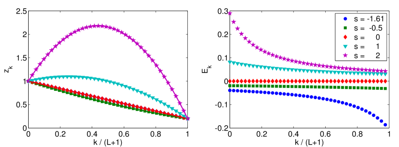
Figure 4: The fugacity profile $z_{k}$ (left) and the effective field $E_{k}$ (right) for a symmetric ZRP with $p=q=1/2$, $z_{l}=1$, $z_{r}=0.2$, and $L=40$. Several values of $s$ are plotted including the typical profile of the unconditioned process ($s=0$) where the fugacity profile is linear. When $s=-\Delta\mu\approx-1.61$, the fugacity profile is linear again (and coincides with that of $s=0$), but the corresponding effective field is non-zero and space-dependent. Solid lines correspond to the macroscopic result, Eq. (124).

3.4.4 Totally asymmetric ZRP

Consider $q=\gamma=\delta=0$ where particles can jump only to the right. One has $A=1$ and $B=0$ (which is always true if $\gamma=0$). On the other hand, $C=\alpha\rme^{s}/p$ and $Da^{k}=0$ for $1\leq k\leq L-1$ and $Da^{L}=\alpha\rme^{s}(p-\beta)/(p\beta)$. Therefore

$$x_{k}=z_{k} = \alpha\rme^{s}/p\quad(1\leq k\leq L-1)$$ (80)

$$x_{L}=z_{L} = \alpha\rme^{s}/\beta.$$ (81)

For the current one has

$$j^{\ast}(s)=\alpha\rme^{s}.$$ (82)

As above one may parametrize the boundary rates in terms of boundary fugacities $\alpha=z_{l}p$ and $\beta=z_{r}p$. Then $z_{k}=z_{L}\rme^{s}$ for $1\leq k\leq L-1$ and $z_{L}=z_{l}\rme^{s}/z_{r}$. For the totally asymmetric case, the effective dynamics is that of the original process, but with an effective reservoir fugacity $z_{l}^{{\mathrm{eff}}}=z_{l}\rme^{s}$.

3.5 Spatial condensation patterns

At this point we recall that the construction presented above is valid only for normalizable left and right eigenvectors, i.e., if $\mbox{$\langle\,{Y}\,|\,{P_{0}}\,\rangle$}<\infty$ for any given initial distribution $|\,{P_{0}}\,\rangle$, $\mbox{$\langle\,{S}\,|\,{X}\,\rangle$}<\infty$ and $Z_{k}<\infty$. In particular, this is the case for non-interacting particles where $z_{k}$ is the stationary local density. On the other hand, depending on the choice of model parameters, the normalization condition can be violated. In this case, a stationary distribution does not exist and one expects the emergence of condensates [30, 31, 34]. It is intriguing that because of the space-dependence of the local fugacities the existence of such condensates will generically depend on the lattice site $k$ and condensates may form in the bulk of the system.

To illustrate how conditioning on atypical currents may lead to condensation we focus on the example of symmetric hopping rates, as described in section 3.4.3, and further restrict the case of baths with equal fugacities, $z_{l}=z_{r}=z_{0}$. Assume that these bath fugacities are subcritical, i.e., $z_{0}<z_{c}$, where $z_{c}$ is the radius of convergence of the sum (9). The unconditioned process, with $s=0$, has a flat fugacity profile, while any $s\neq 0$ leads to a quadratic profile (79) whose maximum is attained at site $k=(L+1)/2$ and equals $z_{(L+1)/2}=z_{0}\cosh^{2}(s/2)$. Thus, a steady state distribution exists only if $|s|<\sqrt{\mathrm{arccosh}(2z_{c}/z_{0})}$, and for larger $|s|$ a condensate forms in the middle of the system. Similar condensation transitions occur when conditioning systems with unequal reservoir fugacities, or with asymmetric hopping. In all these cases, the condensates form in the bulk and their exact location is dictated by the maximum of the fugacity profile.

We expect the supercritical phase to be composed of condensates within the bulk which continually accumulate particles, coexisting with a stationary “fluid” with a finite density. The exact pattern of these condensates is beyond the scope of the present paper.

3.6 Thermodynamic limit

Consider the limit $L\to\infty$ with asymmetry $a>1$ fixed and define the macroscopic space variable $r=r_{k}$. For $r\neq 0,1$ one obtains $y(r)=1$ and $z(r)=\alpha\rme^{s}/(p-q+\gamma)=:z^{\ast}$ independent of $r$. The stationary current of the effective process becomes $j^{\ast}=(p-q)z^{\ast}$. Therefore the effective process in the thermodynamic limit is a ZRP with constant bulk hopping rates $p,q$ as the original process, but effective left injection rate $\alpha^{\mathrm{eff}}=\alpha\rme^{s}$. However, there are in general boundary regions of width $\xi=1/\log{a}$ sites with spatially decaying local driving field and associated non-trivial exponentially decaying boundary layers of the fugacity.

In the symmetric case the localization length $\xi$ diverges. One has $y(r)=r+\rme^{-s}(1-r)$ which leads to an algebraically decaying local drift [see (78)]

$$E(r)=\frac{4\sinh(s/2)}{L[\rme^{s/2}\,r+\rme^{-s/2}\,(1-r)]}$$ (83)

(the $L^{-1}$ factor indicates weakly asymmetric hopping, as discussed below). Therefore, for any $s\neq 0$ the effective ZRP has space-dependent hopping rates. The fugacity takes the form

$$z(r)=\frac{\alpha}{\gamma}+\left(\frac{\delta}{\beta}-\frac{\alpha}{\gamma}\right)\rme^{-s}r+(1-\rme^{-s})\left(\frac{\delta}{\beta}-\frac{\alpha}{\gamma}\rme^{s}\right)r^{2}.$$ (84)

For general $s$ this has a quadratic term which does not exist in the ZRP with space-independent hopping rates. Even when the fugacity profile is linear this is generated by space-dependent hopping rates.

One may also consider the case of weakly asymmetric hopping rates, where the asymmetry scales as $p-q=\nu/L$. Such rates correspond to a driving field which varies substantially only on a macroscopic length scale. Taking the $L\to\infty$ limit of Eq. (67), and noting that in this limit $\tilde{\nu}\to\nu/2q$, yields

$$E(r)=\frac{2\nu\bigl{(}\rme^{s+\nu}\cosh[\nu r]-\cosh[\nu(1-r)]\bigr{)}}{L\bigl{(}\rme^{s+\nu}\sinh[\nu r]+\sinh[\nu(1-r)]\bigr{)}}$$ (85)

(here the result is presented for $q=1/2$ to simplify notation). Other properties of weakly asymmetric systems are considered in more detail in Section 4 below.

3.7 Time-reversed effective dynamics

The adjoint (time-reversed) dynamics of a process with generator $\hat{H}$ is generally defined by $\hat{H}^{\ast}=\hat{P}^{\ast}\hat{H}^{T}(\hat{P}^{\ast})^{-1}$ where the diagonal matrix $\hat{P}^{\ast}$ of stationary probabilities is given by $\hat{P}^{\ast}\mbox{$|\,{\mathbf{S}}\,\rangle$}=\mbox{$|\,{P^{\ast}}\,\rangle$}$ for a stationary probability vector $|\,{P^{\ast}}\,\rangle$ and transposed summation vector $\mbox{$|\,{\mathbf{S}}\,\rangle$}=(\mbox{$\langle\,{\mathbf{S}}\,|$})^{T}$. The system satisfies detailed balance when $\hat{H}=\hat{H}^{\ast}$. This is equivalent to time-reversibility and implies the absence of macroscopic currents. In general, however, the absence of macroscopic currents does not imply detailed balance. In this section we show that in our system the absence of currents does in fact imply detailed balance.

Here, since $\hat{P}^{\ast}=\hat{D}\hat{\Gamma}$, where $\hat{\Gamma}$ has the components of the right eigenvector of $\hat{H}(s)$, one has

$$\hat{G}^{\ast}(s)=\hat{\Gamma}(s)\hat{H}^{T}(s)\hat{\Gamma}^{-1}(s)-\epsilon_{0}(s).$$ (86)

Observe that

$$\hat{\Gamma}(\hat{a}^{+}_{k})^{T}\hat{\Gamma}^{-1}=x_{k}^{-1}\hat{a}^{-}_{k},\quad\hat{\Gamma}(\hat{a}^{-}_{k})^{T}\hat{\Gamma}^{-1}=x_{k}\hat{a}^{+}_{k}.$$ (87)

Therefore

$$-\hat{\Gamma}h^{T}_{k}\hat{\Gamma}^{-1} = p\left(\frac{x_{k}}{x_{k+1}}\hat{a}_{k}^{+}\hat{a}_{k+1}^{-}-\hat{d}_{k}\right)+q\left(\frac{x_{k+1}}{x_{k}}\hat{a}_{k}^{-}\hat{a}_{k+1}^{+}-\hat{d}_{k+1}\right)$$

$$= q\frac{x_{k+1}}{x_{k}}\left(\hat{a}_{k}^{-}\hat{a}_{k+1}^{+}-\hat{d}_{k}\right)+p\frac{x_{k}}{x_{k+1}}\left(\hat{a}_{k}^{+}\hat{a}_{k+1}^{-}-\hat{d}_{k+1}\right)$$

$$+(px_{k}-qx_{k+1})\left(\frac{\hat{d}_{k+1}}{x_{k+1}}-\frac{\hat{d}_{k}}{x_{k}}\right)$$

$$= q\frac{x_{k+1}}{x_{k}}\left(\hat{a}_{k}^{-}\hat{a}_{k+1}^{+}-\hat{d}_{k}\right)+p\frac{x_{k}}{x_{k+1}}\left(\hat{a}_{k}^{+}\hat{a}_{k+1}^{-}-\hat{d}_{k+1}\right)$$

$$+C\left(\frac{\hat{d}_{k+1}}{x_{k+1}}-\frac{\hat{d}_{k}}{x_{k}}\right)$$

and for the boundaries

$$-\hat{\Gamma}h^{T}_{0}\hat{\Gamma}^{-1} = \alpha(x_{1}^{-1}\rme^{s}\hat{a}_{1}^{-}-1)+\gamma(x_{1}\rme^{-s}\hat{a}_{1}^{+}-\hat{d}_{1})$$

$$= \alpha x_{1}^{-1}\rme^{s}(\hat{a}_{1}^{-}-\hat{d}_{1})+\gamma x_{1}\rme^{-s}(\hat{a}_{1}^{+}-1)+(\alpha x_{1}^{-1}\rme^{s}-\gamma)\hat{d}_{1}+\gamma x_{1}\rme^{-s}-\alpha$$

$$= \gamma x_{1}\rme^{-s}(\hat{a}_{1}^{+}-1)+\alpha x_{1}^{-1}\rme^{s}(\hat{a}_{1}^{-}-\hat{d}_{1})+C\left(\frac{\hat{d}_{1}}{x_{1}}-\rme^{-s}\right).$$

and

$$-\hat{\Gamma}\hat{h}_{L}\hat{\Gamma}^{-1} = \delta(x_{L}^{-1}\hat{a}_{L}^{-}-1)+\beta(x_{L}\hat{a}^{+}_{L}-\hat{d}_{L})$$

$$= \beta x_{L}(\hat{a}_{L}^{+}-1)+\delta x_{L}^{-1}(\hat{a}^{-}_{L}-\hat{d}_{L})+\beta x_{L}-\delta+(\delta x_{L}^{-1}-\beta)\hat{d}_{L}$$

$$= \beta x_{L}(\hat{a}_{L}^{+}-1)+\delta x_{L}^{-1}(\hat{a}^{-}_{L}-\hat{d}_{L})+C\left(1-\frac{\hat{d}_{L}}{x_{L}}\right).$$

Therefore, by the telescopic property of the sum and (43) one gets the effective adjoint dynamics

$$\hat{G}^{(0)\ast}(s) = -\sum_{k=1}^{L-1}\left[q\frac{x_{k+1}}{x_{k}}\left(\hat{a}_{k}^{-}\hat{a}_{k+1}^{+}-\hat{d}_{k}\right)+p\frac{x_{k}}{x_{k+1}}\left(\hat{a}_{k}^{+}\hat{a}_{k+1}^{-}-\hat{d}_{k+1}\right)\right]$$

$$-\left[\gamma x_{1}\rme^{-s}(\hat{a}_{1}^{+}-1)+\alpha x_{1}^{-1}\rme^{s}(\hat{a}_{1}^{-}-\hat{d}_{1})\right]$$

$$-\left[\beta x_{L}(\hat{a}_{L}^{+}-1)+\delta x_{L}^{-1}(\hat{a}^{-}_{L}-\hat{d}_{L})\right]$$

This is a driven ZRP with a spatially varying driving field $E_{k}=-\log{a}+2\log{x_{k+1}/x_{k}}$. By comparing transition rates one finds detailed balance $\hat{G}^{(0)\ast}(s)=\hat{G}^{(0)}(s)$ if and only if the stationary current (52) vanishes. Hence, for the conditioned model, the absence of a macroscopic current also implies detailed balance.

4 Atypical current events via macroscopic fluctuation theory

It is our aim in this section to relate the exact microscopic results obtained above to the optimal profiles for a large deviation of the current as obtained from the macroscopic fluctuation theory (MFT) [5]. Since the effective dynamics does not depend on site $k$ of the local conditioning we shall consider here global large deviations of the global time-integrated current in the whole lattice.

The MFT can only deal with symmetric or weakly asymmetric hopping where we set

$$p-q=\nu/L$$ (92)

and $\nu$ is kept fixed in the thermodynamic limit of $L\to\infty$. In what follows we employ the notation defined in (58)–(60). To conform with conventional notations in studies of the MFT, in this section $x$ (rather than $r$) denotes the macroscopic location along the system.

4.1 Fluctuating hydrodynamic description

In the limit of $L\to\infty$, and rescaling space as $x=k/L$ ($0\leq x\leq 1$) and time as $1/L^{2}$, the evolution of the ZRP may be described using a fluctuating hydrodynamic equation. In this description, the density $\rho(x,t)$ evolves according to the continuity equation

$$\dot{\rho}(x,t)=-\frac{\partial j(x,t)}{\partial x},$$ (93)

where $j(x,t)$ is a fluctuating current. The current is given by

$$j(x,t)=-D(\rho)\frac{\partial\rho}{\partial x}+\nu\sigma(\rho)+\sqrt{\sigma(\rho)}\xi(x,t),$$ (94)

where $\xi$ is a standard white noise, and $D(\rho)$, $\sigma(\rho)$ are drift and diffusion coefficients. The validity of the fluctuating hydrodynamics description is based on an assumption of local equilibrium [10], i.e., around each site $k=Lx$ there is “box” of size $1\ll\ell\ll L$ sites which, during times which are much larger than $\ell^{2}$ but much shorter than $L^{2}$ (in the original time units, rather than the rescaled ones), is approximately at equilibrium with density $\rho(x)$. This assumption explains why only equilibrium and linear response coefficients ($D$ and $\sigma$) enter the macroscopic evolution equation.

For the weakly asymmetric ZRP defined above with $q=1/2$ and $p$ as in (92) it is possible to show [7, 38] that

$$D(\rho)=\frac{1}{2}\frac{\partial z(\rho)}{\partial\rho}$$ (95)

and

$$\sigma(\rho)=z(\rho),$$ (96)

where $z(\rho)$ is found by inverting the relation (11) with (9).

4.2 Current large deviations

Assume that during a long period of time $T$, an atypical mean current $j$ was observed to flow through the system. What is the probability for such an event to happen, and what is the most likely density profile conditioned on such an event? These questions can be answered in the limit of $L\to\infty$ for a general driven diffusive system which is described by Eqs. (93)–(94) by using the macroscopic fluctuation theory [5] and the additivity principle [7, 10, 38, 39, 1].

The probability to see an atypical mean current $j$ during a time window $T$ has a large deviations form

$$P(j)\sim\rme^{-TF(j)}.$$ (97)

Assuming that the most probable way to generate this large deviations event is by a static density profile $\rho^{*}(x)$, the large deviations function $F(j)$ is given by

$$F(j)=\min_{\rho(x)}\int_{0}^{1}\frac{[j+D(\rho)\frac{d\rho}{dx}-\nu\sigma(\rho)]^{2}}{2\sigma(\rho)}\,dx.$$ (98)

The minimization is over all profiles which satisfy the boundary conditions dictated by the boundary reservoirs

$$\rho(0) = \rho_{l}\equiv\rho(z_{l})$$

$$\rho(1) = \rho_{r}\equiv\rho(z_{r}),$$ (99)

where $\rho(z)$ is given in Eqs. (11) and (9). The typical profile $\rho^{*}(x)$ is then precisely the profile for which this minimum is achieved.

In our case, it will prove useful to describe the optimal profile using the fugacity profile $z(x)$ rather than the density. The two are related by their usual equilibrium relation, which for the ZRP is given in Eqs. (11) and (9). Using the fluctuation-dissipation relation [39]

$$D(\rho)=\frac{1}{2}\frac{d\log z}{d\rho}\,\sigma(\rho),$$ (100)

one can transform the current large deviations function to

$$F(j)=\min_{z(x)}\tilde{F}[z(x),j]\equiv\min_{z(x)}\int_{0}^{1}\frac{[j+\frac{\sigma(z)}{2z}\frac{dz}{dx}-\nu\sigma(z)]^{2}}{2\sigma(z)}dx.$$ (101)

The boundary conditions now read $z(0)=z_{l}$ and $z(1)=z_{r}$. The optimal fugacity profile $z^{*}(x)$ is the one for which the minimum is achieved, and the optimal density profile is $\rho^{*}(x)=\rho(z^{*}(x))$.

A general solution of the ensuing optimization problem can be obtained as follows [38, 39]. The functional $\tilde{F}$ can be rewritten as

$$\tilde{F}[z(x),j]=\int_{0}^{1}\Bigl{[}W(z)+V(z)\Bigl{(}\frac{dz}{dx}\Bigr{)}^{2}\Bigr{]}dx+\int_{z_{l}}^{z_{r}}\frac{j-\nu\sigma(z^{\prime})}{2z^{\prime}}dz^{\prime}-j\nu,$$ (102)

where

$$V(z)=\frac{\sigma(z)}{8z^{2}},\qquad{\mbox{and}}\qquad W(z)=\frac{j^{2}}{2\sigma(z)}+\frac{\nu^{2}\sigma(z)}{2}.$$ (103)

Performing the functional derivative of $\tilde{F}$ yields

$$0=\frac{\delta\tilde{F}}{\delta{z}}=\frac{dW}{dz}-\frac{dV}{dz}\Bigl{(}\frac{dz}{dx}\Bigr{)}^{2}-2V(z)\frac{d^{2}z}{dx^{2}}.$$ (104)

Multiplying this equation by $dz/dx$ one obtains

$$\frac{d}{dx}\Bigl{[}W(z)-V(z)\Bigl{(}\frac{dz}{dx}\Bigr{)}^{2}\Bigr{]}=0,$$ (105)

which upon integrating yields the differential equation

$$\frac{dz}{dx}=\pm\sqrt{\frac{W(z)+\tilde{K}}{V(z)}}=\pm\frac{2jz}{\sigma(z)}\sqrt{\Bigl{(}1+\frac{\nu\sigma(z)}{j}\Bigr{)}^{2}+K\sigma(z)}.$$ (106)

Here $K$ and $\tilde{K}$ are integration constants which are related by $\tilde{K}=j^{2}K/2+j\nu$. They are determined by the boundary condition $z(1)=z_{r}$. Using (106) one may simplify a bit expression (102) evaluated at the optimal profile:

$$F(j)=2\int_{0}^{1}W(z^{*})dx+\int_{z_{l}}^{z_{r}}\frac{j-\nu\sigma(z^{\prime})}{2z^{\prime}}dz^{\prime}+\frac{j^{2}K}{2}.$$ (107)

4.3 Optimal profile for the ZRP

Substituting the drift and diffusion coefficients (95) and (96) in (106) yields the ordinary differential equation

$$\frac{dz}{dx}=\pm 2j\sqrt{\Bigl{(}1+\frac{\nu z}{j}\Bigr{)}^{2}+Kz}.$$ (108)

As in the microscopic calculation, the fugacity profile is independent of the rates $u(n)$, while the density profile depends on the form of $u(n)$ through (11) and (9).

The solution of (108) with the boundary conditions $z(0)=z_{l}$ and $z(1)=z_{r}$ is

$$z^{*}(x)=z_{0}\frac{\rme^{\frac{\Delta\mu}{2}}\sinh^{2}[\nu(1-x)]+\rme^{-\frac{\Delta\mu}{2}}\sinh^{2}[\nu x]+2Q\sinh[\nu x]\sinh[\nu(1-x)]}{\sinh^{2}\nu},$$ (109)

with

$$Q\equiv\sqrt{1+\Bigl{(}\frac{j\sinh\nu}{z_{0}\nu}\Bigr{)}^{2}}.$$ (110)

When integrating Eq. (108), the boundary condition $z(1)=z_{r}$ was used to find that

$$K=-\frac{2\nu}{j}\Bigl{[}1+\frac{z_{0}\nu}{j\sinh\nu}\Bigl{(}Q\coth\nu-\frac{\cosh(\Delta\mu/2)}{\sinh\nu}\Bigr{)}\Bigr{]}.$$ (111)

An interesting limit is that of a symmetric ZRP, in which $\nu\to 0$. Taking this limit in Eq. (109) yields the simpler quadratic expression

$$z^{*}_{\nu=0}(x)=z_{0}\bigl{[}e^{\frac{\Delta\mu}{2}}(1-x)^{2}+\rme^{-\frac{\Delta\mu}{2}}x^{2}+2x(1-x)\sqrt{1+(j/z_{0})^{2}}\bigr{]}.$$ (112)

This expression simplifies further in the equilibrium case where $z_{l}=z_{r}$, i.e., ${\Delta\mu=0}$:

$$z^{*}_{\nu,\Delta\mu=0}(x)=z_{0}\bigl{[}1+2x(1-x)\bigl{(}\sqrt{1+(j/z_{0})^{2}}-1\bigr{)}\bigr{]}.$$ (113)

Note that according to (109) the fugacity profile (and hence the density profile) is symmetric around $x=1/2$ whenever $z_{l}=z_{r}$, or equivalently $\Delta\mu=0$, even when the bulk dynamics is asymmetric (i.e., when $\nu\neq 0$).

4.4 Optimal profile in the $s$-ensemble

As discussed above, rather than considering a system conditioned on a specific value of the current, one may move to an ensemble in which the current is allowed to fluctuate but is “tilted” towards this atypical value. Formally, this is done by considering the cumulant generating function of the current,(i.e., its log-Laplace transform) $G(s)$, defined as

$$\rme^{TG(s)}\equiv\bigl{\langle}\rme^{sTj}\bigr{\rangle}\sim\int dj\,\rme^{T[sj-F(j)]},$$ (114)

where (97) was used. The last integral is dominated, in the large $T$ limit, by its saddle point, and therefore $G(s)$ is the Legendre transform

$$G(s)=\max_{j}[sj-F(j)].$$ (115)

In this grandcanonically conditioned “$s$-ensemble”, the optimal profile for a given value of $s$ is exactly the optimal profile for the value $j(s)$ at which the maximum in Eq. (115) is attained (this is nothing but the equivalence of the two ensembles). This value can be found by inverting the relation

$$s(j)=F^{\prime}(j).$$ (116)

We shall now carry out this computation for the ZRP. Note that the current $j$ enters the optimal profile (109) only through $Q$ given by (110), and therefore obtaining $Q(s)$ is goal of the current calculation.

The first step is to find $F(j)$, by substituting the optimal profile in (107). Carrying out the integrals, one finds

$$\int_{0}^{1}z^{*}(x)dx=\frac{z_{0}}{\nu\sinh\nu}\Bigl{[}Q(\nu\coth\nu-1)+\cosh(\Delta\mu/2)\Bigl{(}\cosh\nu-\frac{\nu}{\sinh\nu}\Bigr{)}\Bigr{]},$$ (117)

and

$$\int_{0}^{1}\frac{dz}{z^{*}(x)}=\frac{1}{j}\log[Q+\sqrt{Q^{2}-1}].$$ (118)

For the ZRP, one also obtains

$$\int_{z_{l}}^{z_{r}}\frac{j-\nu\sigma(z^{\prime})}{2z^{\prime}}dz^{\prime}=\int_{z_{l}}^{z_{r}}\frac{jdz^{\prime}}{2z^{\prime}}+\frac{\nu(z_{l}-z_{r})}{2}=$$ (119)

$$=\frac{\nu(z_{l}-z_{r})}{2}-\frac{j}{2}\log\Bigl{(}\frac{z_{l}}{z_{r}}\Bigr{)}=z_{0}\nu\sinh\Bigl{(}\frac{\Delta\mu}{2}\Bigr{)}-j\frac{\Delta\mu}{2}.$$ (120)

Combining Eqs. (103), (107), (111) and (117)–(119) yields

$$F(j)=\frac{z_{0}\nu}{\sinh\nu}\Bigl{[}\cosh\Bigl{(}\frac{\Delta\mu}{2}+\nu\Bigr{)}-Q-\sqrt{Q^{2}-1}\log\bigl{(}\sqrt{Q^{2}-1}+Q\bigr{)}\Bigr{]}.$$ (121)

Then, using (116), we find

$$j(s)=\frac{z_{0}\nu}{\sinh\nu}\sinh\Bigl{(}s+\frac{\Delta\mu}{2}+\nu\Bigr{)}.$$ (122)

Finally, substituting in (110) yields the simple expression

$$Q=\cosh\Bigl{(}s+\frac{\Delta\mu}{2}+\nu\Bigr{)},$$ (123)

which together with (109) yields the optimal fugacity profile for a given value of $s$. As before, it is interesting to consider the symmetric limit of $\nu=0$. In this case,

$$z^{*}_{\nu=0}(x)=z_{0}\bigl{[}\rme^{\frac{\Delta\mu}{2}}(1-x)^{2}+\rme^{-\frac{\Delta\mu}{2}}x^{2}+2\cosh\Bigl{(}s+\frac{\Delta\mu}{2}\Bigr{)}x(1-x)\bigr{]}.$$ (124)

4.5 Comparison with the microscopic calculation

As discussed in Section 3.6, in the weakly asymmetric limit of (92) with $q=1/2$, and when $L\to\infty$, one has $\tilde{\nu}\to\nu$ [where $\tilde{\nu}$ is the asymmetry parameter defined in (57)]. Therefore, in this limit the microscopic fugacity profile (69)–(70) is precisely the same as the macroscopic expressions (109) and (123). Similarly, the macroscopic expression (122) for the current in the $s$-ensemble coincides in this limit with exact expression (71) obtained for barrier-free reservoir coupling with weak asymmetry. Indeed, figures 3 and 4 present fugacity profiles for symmetric and weakly-asymmetric hopping and several values of $s$, and demonstrate the agreement between the microscopic and macroscopic results.

An interesting observation is that the microscopic expression (69) for the optimal profile and macroscopic one (109) have the same functional form even when $L$ is small and the asymmetry is not weak, provided one uses the definition $x=k/(L+1)$. In particular, by substituting $\nu=cL$ in the macroscopic profile (109) (with a constant $c$) it is possible to obtain the correct profile for strongly asymmetric hopping (i.e., with $p\neq q$ independent of $L$). However, using the macroscopic theory beyond its limit of validity comes with a price: The precise value of the prefactor $c$ which corresponds to given values of $p$ and $q$ cannot be determined within the macroscopic approach, and only the microscopic one yields equation (57).

References

• Derrida [2007] B. Derrida. Non-equilibrium steady states: fluctuations and large deviations of the density and of the current. J. Stat. Mech., 7:23, July 2007.
• Blythe and Evans [2007] R. A. Blythe and M. R. Evans. Nonequilibrium steady states of matrix-product form: a solver’s guide. J. Phys. A, 40:333, November 2007.
• Schadschneider et al. [2010] A. Schadschneider, D. Chowdhury, and K. Nishinari. Stochastic Transport in Complex Systems: From Molecules to Vehicles. Elsevier Science, Amsterdam, 2010.
• Chou et al. [2011] T. Chou, K. Mallick, and R. K. P. Zia. Non-equilibrium statistical mechanics: from a paradigmatic model to biological transport. Rep. Prog. Phys., 74(11), 2011.
• Bertini et al. [2015] L. Bertini, A. De Sole, D. Gabrielli, G. Jona-Lasinio, and C. Landim. Macroscopic fluctuation theory. To appear in Rev. Mod. Phys., 2015.
• Derrida et al. [2002] B. Derrida, J. L. Lebowitz, and E. R. Speer. Large Deviation of the Density Profile in the Steady State of the Open Symmetric Simple Exclusion Process. J. Stat. Phys., 107:599–634, May 2002.
• Bertini et al. [2002] L. Bertini, A. de Sole, D. Gabrielli, G. Jona-Lasinio, and C. Landim. Macroscopic Fluctuation Theory for Stationary Non-Equilibrium States. J. Stat. Phys., 107:635–675, May 2002.
• Liggett [1999] T. M. Liggett. Stochastic Interacting Systems: Contact, Voter and Exclusion Processes. Springer, Berlin, 1999.
• Schütz [2001] G. M. Schütz. Exactly solvable models for many-body systems far from equilibrium. volume 19 of Phase Transitions and Critical Phenomena, pages 1–251. Academic Press, 2001.
• Bodineau and Derrida [2005] T. Bodineau and B. Derrida. Distribution of current in nonequilibrium diffusive systems and phase transitions. Phys. Rev. E, 72(6):066110, December 2005.
• Hurtado and Garrido [2011] P. I. Hurtado and P. L. Garrido. Spontaneous Symmetry Breaking at the Fluctuating Level. Phys. Rev. Lett., 107(18):180601, October 2011.
• Espigares et al. [2013] C. P. Espigares, P. L. Garrido, and P. I. Hurtado. Dynamical phase transition for current statistics in a simple driven diffusive system. Phys. Rev. E, 87(3):032115, March 2013.
• Bodineau and Derrida [2006] T. Bodineau and B. Derrida. Current Large Deviations for Asymmetric Exclusion Processes with Open Boundaries. J. Stat. Phys., 123:277–300, April 2006.
• Simon [2009] D. Simon. Construction of a coordinate Bethe ansatz for the asymmetric simple exclusion process with open boundaries. J. Stat. Mech., 7:17, July 2009.
• Belitsky and Schütz [2013a] V. Belitsky and G. M. Schütz. Microscopic Structure of Shocks and Antishocks in the ASEP Conditioned on Low Current. J. Stat. Phys., 152:93–111, July 2013a.
• Belitsky and Schütz [2013b] V. Belitsky and G. M. Schütz. Antishocks in the ASEP with open boundaries conditioned on low current. J. Phys. A, 46:295004, July 2013b.
• [17] G. M. Schütz. Duality relations for the ASEP conditioned on a low current. (work in progress).
• Miller [1961] H. D. Miller. A convexity property in the theory of random variables defined on a finite markov chain. Ann. Math. Statist., 32(4):1260–1270, 12 1961.
• G. and D. [1994] Rogers L. C. G. and Williams D. Diffusions, Markov Processes, and Martingales. Vol. 1: Foundations. Wiley, 1994.
• Jack and Sollich [2010] R. L. Jack and P. Sollich. Large Deviations and Ensembles of Trajectories in Stochastic Models. Prog. Theor. Phys. Suppl., 184:304–317, 2010.
• Chetrite and Touchette [2013] R. Chetrite and H. Touchette. Nonequilibrium Microcanonical and Canonical Ensembles and Their Equivalence. Phys. Rev. Lett., 111(12):120601, September 2013.
• Sasamoto and Spohn [2010] T. Sasamoto and H. Spohn. One-Dimensional Kardar-Parisi-Zhang Equation: An Exact Solution and its Universality. Phys. Rev. Lett., 104(23):230602, June 2010.
• Popkov et al. [2010] V. Popkov, G. M. Schütz, and D. Simon. ASEP on a ring conditioned on enhanced flux. J. Stat. Mech., 2010:P10007, 2010.
• Popkov and Schütz [2011] V. Popkov and G. M. Schütz. Transition Probabilities and Dynamic Structure Function in the ASEP Conditioned on Strong Flux. J. Stat. Phys., 142:627–639, February 2011.
• Schütz [2015] G. M. Schütz. The Space-Time Structure of Extreme Current and Activity Events in the ASEP. In B. Aneva and M. Kouteva-Guentcheva, editors, Nonlinear Mathematical Physics and Natural Hazards, volume 163 of Springer Proceedings in Physics, pages 13–28. Springer International Publishing, 2015. ISBN 978-3-319-14327-9.
• [26] D. Karevski and G. M. Schütz. Conformal invariance in stochastic particles conditioned on an atypical current. (work in progress).
• Spitzer [1970] Frank Spitzer. Interaction of markov processes. Adv. Math., 5(2):246–290, 1970.
• Evans and Hanney [2005] M. R. Evans and T. Hanney. Nonequilibrium statistical mechanics of the zero-range process and related models. J. Phys. A, 38:R195–R240, May 2005.
• Levine et al. [2005] E. Levine, D. Mukamel, and G. M. Schütz. Zero-Range Process with Open Boundaries. Journal of Statistical Physics, 120:759–778, September 2005.
• Harris et al. [2006] R. J. Harris, A. Rákos, and G. M. Schütz. Breakdown of Gallavotti-Cohen symmetry for stochastic dynamics. EPL, 75:227–233, July 2006.
• Rákos and Harris [2008] A. Rákos and R. J. Harris. On the range of validity of the fluctuation theorem for stochastic Markovian dynamics. J. Stat. Mech., 5:P05005, May 2008.
• Gallavotti and Cohen [1995] G. Gallavotti and E. G. D. Cohen. Dynamical ensembles in stationary states. J. Stat. Phys., 80:931–970, September 1995.
• Lebowitz and Spohn [1999] J. L. Lebowitz and H. Spohn. A Gallavotti-Cohen-Type Symmetry in the Large Deviation Functional for Stochastic Dynamics. J. Stat. Phys., 95:333–365, April 1999.
• Harris et al. [2013] R. J. Harris, V. Popkov, and G. M. Schütz. Dynamics of instantaneous condensation in the zrp conditioned on an atypical current. Entropy, 15(11):5065–5083, 2013.
• Lloyd, P. and Sudbury, A. and Donnelly, P. [1996] Lloyd, P. and Sudbury, A. and Donnelly, P. Quantum operators in classical probability theory: I. “quantum spin” techniques and the exclusion model of diffusion. Stoch. Processes Appl., 61(2):205–221, 1996.
• Derrida and Lebowitz [1998] B. Derrida and J. L. Lebowitz. Exact Large Deviation Function in the Asymmetric Exclusion Process. Phys. Rev. Lett., 80:209–213, January 1998.
• Harris and Schütz [2007] R. J. Harris and G. M. Schütz. Fluctuation theorems for stochastic dynamics. J. Stat. Mech., 7:20, July 2007.
• Bodineau and Derrida [2004] T. Bodineau and B. Derrida. Current Fluctuations in Nonequilibrium Diffusive Systems: An Additivity Principle. Phys. Rev. Lett., 92(18):180601, May 2004.
• Bodineau and Derrida [2007] T. Bodineau and B. Derrida. Cumulants and large deviations of the current through non-equilibrium steady states. Comptes Rendus Physique, 8:540–555, June 2007.