SI-HEP-2015-10  QFET-2015-11

1 Introduction

The first measurement of the $B^{+}\to\pi^{+}\mu^{+}\mu^{-}$ decay by the LHCb Collaboration [1] paved the way for more detailed measurements of $b\to d\ell^{+}\ell^{-}$ decays. These results will complement the available data on $b\to s\ell^{+}\ell^{-}$ decays, providing new important insight in the dynamics of flavour-changing neutral-current (FCNC) transitions in Standard Model (SM) and beyond.

One important feature of exclusive $b\to d\ell^{+}\ell^{-}$ decays is a non-vanishing direct CP-asymmetry. In Standard Model (SM) this effect is caused by the interference between the dominant short-distance contributions of semileptonic and magnetic dipole operators and the contributions of other effective operators accompanied by the electromagnetic lepton-pair emission. The amplitudes of the latter contributions are process-dependent, and are defined as hadronic matrix elements of nonlocal operator products. Importantly, the parts of the exclusive $b\to d\ell^{+}\ell^{-}$ decay amplitudes proportional to $\lambda_{u}\equiv V_{ub}V^{*}_{ud}$ and $\lambda_{c}\equiv V_{cb}V^{*}_{cd}$ are of the same order of Cabibbo suppression and, in addition to a relative CKM phase, have different strong phases originating from the nonlocal amplitudes. The main goal of this work is to calculate the hadronic matrix elements of nonlocal contributions to $B\to\pi\ell^{+}\ell^{-}$ at large recoil of the pion, that is, at small and intermediate lepton-pair mass, $q^{2}\ll m_{B}^{2}$ .

An advanced theoretical description of the exclusive semileptonic FCNC decays was developed on the basis of QCD factorization (QCDF) approach [2], applied first to the decays $B\to K^{(*)}\ell^{+}\ell^{-}$ in Ref. [3] and to $B\to\rho\ell^{+}\ell^{-}$ in Ref. [4]; see also further applications to $B\to K\ell^{+}\ell^{-}$ [5], and to $B\to\pi\ell^{+}\ell^{-}$ [6]. An approach combining QCD light-cone sum rules with QCDF at $q^{2}>0$ for $B\to K^{(*)}\ell^{+}\ell^{-}$ was used in [7].

In QCDF, the nonlocal effects in these decays are described in terms of hard-scattering quark-gluon amplitudes with virtual photon emission, convoluted with light-cone distribution amplitudes (DAs) of the initial $B$ meson and final light meson. Soft gluons, responsible for the onset of long-distance effects in the channel of the electromagnetic current, including vector resonance formation and nonfactorizable interactions with initial and final meson remain beyond the reach of QCDF. Hence, these contributions have to be kept small, protected by their power suppression. In particular, one avoids the intervals of lepton-pair mass squared $q^{2}$ in the vicinity of vector meson masses, $q^{2}\sim m_{V}^{2}$ ($V=\rho,\omega,...,J/\psi,..$), where nonlocal effects are largely influenced by long-distance quark-gluon dynamics. This constraint defines the region of applicability of QCDF, that is, roughly from $q^{2}_{\rm min}=2\leavevmode\nobreak\ \mbox{GeV}^{2}$ up to $q^{2}_{\rm max}=6\leavevmode\nobreak\ \mbox{GeV}^{2}$. In this region, quark-hadron duality approximation is tacitly assumed for the contributions of radially excited and continuum hadronic states with the quantum numbers of light vector mesons.

Note that in the $B\to\pi\ell^{+}\ell^{-}$ decay, as compared to $B\to K\ell^{+}\ell^{-}$, the role of nonlocal effects related to $\rho$ and $\omega$ resonances in the $q^{2}$ channel grows due to the current-current operators with large Wilson coefficients in the $\sim\lambda_{u}$ part. For the same reason, the weak annihilation combined with virtual photon emission, being suppressed in $B\to K\ell^{+}\ell^{-}$ decays, becomes one of the dominant nonlocal effects in $B\to\pi\ell^{+}\ell^{-}$. In the QCDF approach one describes the weak annihilation contribution [3] in terms of a virtual photon emission off the spectator antiquark in the $B$ meson, followed by the subsequent annihilation to a final pion state. The accuracy of this leading-power diagram approximation, presumably quite sufficient for $B\to K\ell^{+}\ell^{-}$ decay, becomes crucial for $B\to\pi\ell^{+}\ell^{-}$.

In this paper we calculate the nonlocal effects in $B\to\pi\ell^{+}\ell^{-}$, using the method formulated in Ref. [8] and applied in Ref. [9] to $B\to K\ell^{+}\ell^{-}$. One avoids applying QCDF directly in the physical region $q^{2}>0$ and calculates the amplitudes of nonlocal contributions at deep spacelike $q^{2}<0$, $|q^{2}|\gg\Lambda_{QCD}^{2}$, where the operator-product expansion (OPE) and QCDF can safely be used. The OPE contributions include the leading-order (LO) loops and weak annihilation, the NLO perturbative corrections to the loops and hard spectator scattering. Furthermore, we include important nonfactorizable soft-gluon effects via dedicated LCSR calculations of hadronic matrix elements. The amplitudes of nonlocal effects are then represented in a form of hadronic dispersion relations in the variable $q^{2}$ where vector mesons are included explicitly. The residues of vector-meson poles related to nonleptonic $B\to V\pi$ decays are fixed, using experimental data and/or QCDF estimates. The nonresonant part of the hadronic dispersion integral is parametrized combining quark-hadron duality with a polynomial ansatz. Finally, the unknown parameters in the dispersion relation, most importantly, the strong phases of resonance and nonresonant contributions are fitted to the QCD calculation at $q^{2}<0$. The advantage of describing nonlocal contributions to the FCNC decay amplitude in terms of hadronic dispersion relation is that the latter is valid in the whole large-recoil region specified as $4m_{\ell}^{2}<q^{2}<m_{J/\psi}^{2}$.

In $B\to\pi\ell^{+}\ell^{-}$ decays the combinations of CKM factors $\lambda_{u}$ and $\lambda_{c}$ are comparable in size. Correspondingly, we have to calculate separately two hadronic matrix elements of nonlocal effects multiplying $\lambda_{u}$ and $\lambda_{c}$. A similar CKM separation has to be done in the amplitudes of nonleptonic $B\to V\pi$ decays, used to fix the residues of vector-meson poles in the hadronic dispersion relations. To obtain the separate parts of nonleptonic $B\to V\pi$ amplitudes for $V=\rho,\omega$ we employ the QCDF results [10] and control the resulting amplitudes with the data on branching ratios and CP-asymmetries of these nonleptonic decays.

The plan of this paper is as follows. In Sec. 2 we present the structure of the $B\to\pi\ell^{+}\ell^{-}$ decay amplitude and define the hadronic matrix element of nonlocal contributions. Sec. 3 contains a detailed calculation of these amplitudes at $q^{2}<0$. In Sec. 4 we perform the relevant numerical analysis. In Sec. 5 the necessary inputs for the nonleptonic $B\to V\pi$ decay amplitudes are presented. Sec. 6 is devoted to the analysis of the hadronic dispersion relations. Matching the latter to the result of QCD calculation, we then obtain $\Delta C^{(B\pi)}_{9}(q^{2}>0)$. In Sec. 7 our predictions for the observables in the $B\to\pi\ell^{+}\ell^{-}$ decay are presented, including the decay rate, direct $CP$-asymmetry and isospin-asymmetry. In Sec. 8 we estimate the rate for $B\to\pi\nu\bar{\nu}$ decay and Sec. 9. contains the concluding discussion. The two appendices contain: (A) the operators and Wilson coefficients of the effective Hamiltonian of $b\to d\ell^{+}\ell^{-}$ transitions and (B) the QCDF expressions used for the amplitudes of $B\to\rho(\omega)\pi$ nonleptonic decays.

2 The $B\to\pi\ell^{+}\ell^{-}$ decay amplitude

The effective weak Hamiltonian of the $b\to d\ell^{+}\ell^{-}$ transitions $(\ell=e,\mu,\tau)$ has the following form [11, 12] in the SM :

$$H^{b\to d}_{\rm eff}=\frac{4G_{F}}{\sqrt{2}}\left(\lambda_{u}\sum\limits_{i=1}^{2}C_{i}\,{\cal O}_{i}^{u}+\lambda_{c}\sum\limits_{i=1}^{2}C_{i}\,{\cal O}_{i}^{c}-\lambda_{t}\sum\limits_{i=3}^{10}C_{i}\,{\cal O}_{i}\right)+h.c.\,,$$ (1)

where $\lambda_{p}=V_{pb}V_{pd}^{*}$, $(p=u,c,t)$ are the products of CKM matrix elements. In contrast to the $b\to s\ell^{+}\ell^{-}$ transitions, all three terms in the unitary relation have the same order of Cabibbo suppression, $\lambda_{u}\sim\lambda_{c}\sim\lambda_{t}\sim\lambda^{3}$, $\lambda$ being the Wolfenstein parameter. Hereafter, we assume CKM unitarity and replace $\lambda_{t}=-(\lambda_{u}+\lambda_{c})$. The local dimension-6 operators ${\cal O}_{i}$ in (1) together with the numerical values of their Wilson coefficients $C_{i}$ at relevant scales are presented in the Appendix A.

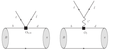
Figure 1: FCNC contributions to $B\to\pi\ell^{+}\ell^{-}$ due to the effective operators $O_{9,10}$ (left) and $O_{7\gamma}$ (right) denoted as black squares.

The amplitude of the $B\to\pi\ell^{+}\ell^{-}$ decay reads:

$$A(B\to\pi\ell^{+}\ell^{-}) = -\langle\pi(p)\ell^{+}\ell^{-}|H_{\rm eff}^{b\to d}|B(p+q)\rangle$$ (2)

$$= \frac{G_{F}}{\sqrt{2}}\frac{\alpha_{\rm em}}{\pi}\lambda_{t}\Biggl{[}\left(\bar{\ell}\gamma^{\mu}\ell\right)p_{\mu}\left(C_{9}f^{+}_{B\pi}(q^{2})+\frac{2m_{b}}{m_{B}+m_{\pi}}C_{7}^{\rm eff}f^{T}_{B\pi}(q^{2})\right)$$

$$+ \left(\bar{\ell}\gamma^{\mu}\gamma_{5}\ell\right)p_{\mu}C_{10}f_{B\pi}^{+}(q^{2})+16\pi^{2}\frac{\bar{\ell}\gamma^{\mu}\ell}{q^{2}}\left(\frac{\lambda_{u}}{\lambda_{t}}{\cal H}_{\mu}^{(u)}+\frac{\lambda_{c}}{\lambda_{t}}{\cal H}_{\mu}^{(c)}\right)\Biggr{]},$$

where $p^{\mu}$ and $q^{\mu}$ are the four-momenta of the $\pi$-meson and lepton pair, respectively.

In (2), the dominant contributions of the operators $O_{9,10}$ and $O_{7\gamma}$ are separated (Fig. 1) and their hadronic matrix elements are expressed in terms of the vector and tensor $B\to\pi$ form factors, $f^{+}_{B\pi}(q^{2})$ and $f^{T}_{B\pi}(q^{2})$, respectively, defined in the standard way:

$$\langle\pi(p)|\bar{d}\gamma^{\mu}b|B(p+q)\rangle=f^{+}_{B\pi}(q^{2})\left[2p^{\mu}+\left(1-\frac{m_{B}^{2}-m_{\pi}^{2}}{q^{2}}\right)q^{\mu}\right]$$

$$+f^{0}_{B\pi}(q^{2})\,\frac{m_{B}^{2}-m_{\pi}^{2}}{q^{2}}\,q^{\mu},$$ (3)

$$\langle\pi(p)|\bar{d}\sigma^{\mu\nu}q_{\nu}b|B(p+q)\rangle=\frac{if^{T}_{B\pi}(q^{2})}{m_{B}+m_{\pi}}\left[2q^{2}p^{\mu}+\bigg{(}q^{2}-\left(m_{B}^{2}-m_{\pi}^{2}\right)\bigg{)}q^{\mu}\right]\,.$$ (4)

For definiteness, hereafter we consider the $B^{-}\to\pi^{-}\ell^{+}\ell^{-}$ mode, unless stated otherwise. We assume isospin symmetry for the $b\to d$ and $b\to u$ transition form factors. The $B^{-}\to\pi^{-}$ form factor $f^{+}_{B\pi}$ in Eq. (2) is equal to the one in the $\bar{B}^{0}\to\pi^{+}\ell^{-}\nu_{\ell}$ semileptonic decay and the form factors in the $\bar{B}^{0}\to\pi^{0}\ell^{+}\ell^{-}$ decay amplitude have an extra factor $1/\sqrt{2}$. For the $CP$-conjugated modes $B^{+}\to\pi^{+}\ell^{+}\ell^{-}$ and $B^{0}\to\pi^{0}\ell^{+}\ell^{-}$, respectively, one has to use the hermitian conjugated effective operators with complex conjugated CKM factors $\lambda_{p}^{*}$.

The current-current, quark-penguin and chromomagnetic operators in the effective Hamiltonian (1) contribute to the decay amplitude (2), with the lepton pair produced via virtual photon. After factorizing out the lepton pair, the expression for these nonlocal effects is arranged in (2) in a form of correlation functions of the time-ordered product of quark operators with the quark e.m. current, $j_{\mu}^{\rm em}=\sum_{q=u,d,s,c,b}Q_{q}\bar{q}\gamma_{\mu}q$, sandwiched between $B$ and $\pi$ states:

$${\cal H}_{\mu}^{(p)} = i\int d^{4}xe^{iqx}\langle\pi(p)|{\rm T}\biggl{\{}j_{\mu}^{\rm em}(x),\biggl{[}C_{1}{\cal O}_{1}^{p}(0)+C_{2}{\cal O}_{2}^{p}(0)$$

$$+ \sum\limits_{k=3-6,8g}C_{k}{\cal O}_{k}(0)\biggr{]}\biggr{\}}|B(p+q)\rangle=\left[(p\cdot q)q_{\mu}-q^{2}p_{\mu}\right]{\cal H}^{(p)}(q^{2}),\leavevmode\nobreak\ \leavevmode\nobreak\ (p=u,c),$$ (5)

where the index $p=u,c$ hereafter distinguishes the hadronic matrix elements in Eq.(2), multiplying, respectively, the CKM factors $\lambda_{u},\lambda_{c}$. Substituting (2) in (2) and taking into account the conservation of the leptonic current, we write down the decay amplitude in a more compact form:

$$A(B\to\pi\ell^{+}\ell^{-})=\frac{G_{F}}{\sqrt{2}}\lambda_{t}\frac{\alpha_{\rm em}}{\pi}f^{+}_{B\pi}(q^{2})\Biggl{[}\left(\bar{\ell}\gamma^{\mu}\ell\right)p_{\mu}\Bigg{(}C_{9}+\Delta C^{(B\pi)}_{9}(q^{2})$$

$$+\frac{2m_{b}}{m_{B}+m_{\pi}}C_{7}^{\rm eff}r_{B\pi}^{T}(q^{2})\Bigg{)}+\left(\bar{\ell}\gamma^{\mu}\gamma_{5}\ell\right)p_{\mu}C_{10}\Biggr{]}\,,$$ (6)

where the invariant amplitudes introduced in Eq. (2) form a process-dependent and $q^{2}$-dependent addition to the Wilson coefficient $C_{9}$:

$$\Delta C_{9}^{(B\pi)}(q^{2})\equiv-16\pi^{2}\frac{\left(\lambda_{u}{\cal H}^{(u)}(q^{2})+\lambda_{c}{\cal H}^{(c)}(q^{2})\right)}{\lambda_{t}f_{B\pi}^{+}(q^{2})}\,.$$ (7)

In Eq.(2) we also introduce the ratio of tensor and vector form factors:

$$r_{B\pi}^{T}(q^{2})\equiv\frac{f_{B\pi}^{T}(q^{2})}{f_{B\pi}^{+}(q^{2})}\,.$$ (8)

In the case of $b\to s\ell^{+}\ell^{-}$ transitions, the factor $\lambda_{u}$ is usually neglected so that $\lambda_{c}=-\lambda_{t}$, and one recovers the corresponding expression for $\Delta C_{9}^{(BK)}(q^{2})$ in $B\to K\ell^{+}\ell^{-}$ used in Ref. [9].

3 Nonlocal effects at spacelike $q^{2}$

In this section we present separate contributions to the nonlocal amplitudes ${\cal H}^{(u)}(q^{2})$ and ${\cal H}^{(c)}(q^{2})$ defined in (2) and calculated at $q^{2}<0$, in the same approximation that was adopted in Ref. [9] for $B\to K\ell^{+}\ell^{-}$.

3.1 Factorizable loops

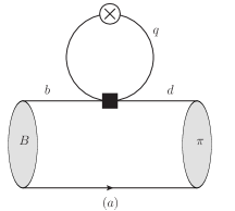
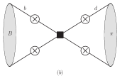
Figure 2: Leading-order diagrams of nonlocal effects in $B\to\pi\ell^{+}\ell^{-}$ due to the four-quark effective operators $O_{1,2}^{u,c}$ and $O_{3-6}$: the quark-loop (a) and weak annihilation (b). The black square denotes the operator and crossed circles indicate possible points of the virtual photon emission.

At leading order (LO) in the quark-gluon coupling, the contributions of the four-quark operators to $B\to\pi\ell^{+}\ell^{-}$ have two possible quark topologies. One of them corresponds to the factorizable quark-loop diagrams with different flavours (see Fig. 2(a)). Their expressions are obtained from, e.g., the ones presented in Ref. [9], separating the $\sim\lambda_{u}$ and $\sim\lambda_{c}$ parts:

$${\cal H}^{(u)}_{\rm fact,LO}(q^{2}) = \frac{1}{12\pi^{2}}\left(\frac{C_{1}}{3}+C_{2}\right)g_{0}(q^{2})f^{+}_{B\pi}(q^{2})+{\cal H}^{(3-6)}_{\rm fact,LO}(q^{2})\,,$$ (9)

$${\cal H}^{(c)}_{\rm fact,LO}(q^{2}) = \frac{1}{12\pi^{2}}\left(\frac{C_{1}}{3}+C_{2}\right)g(q^{2},m_{c}^{2})f^{+}_{B\pi}(q^{2})+{\cal H}^{(3-6)}_{\rm fact,LO}(q^{2})\,,$$ (10)

where the common term stemming from the quark-penguin operators $O_{3-6}$ is

$${\cal H}^{(3-6)}_{\rm fact,LO}(q^{2}) = \frac{1}{24\pi^{2}}\Biggr{[}-\left(\frac{4}{3}C_{3}+\frac{4}{3}C_{4}+C_{5}+\frac{C_{6}}{3}\right)\left(g(q^{2},m_{b}^{2})+g(q^{2},m_{s}^{2})\right)$$ (11)

$$+ 2\left(C_{3}+\frac{1}{3}C_{4}+C_{5}+\frac{C_{6}}{3}\right)g(q^{2},m_{c}^{2})$$

$$+ \left(C_{3}+\frac{C_{4}}{3}+C_{5}+\frac{C_{6}}{3}\right)g_{0}(q^{2})$$

$$+ \left(C_{3}+\frac{C_{4}}{3}+C_{5}+\frac{C_{6}}{3}\right)\Biggl{]}f^{+}_{B\pi}(q^{2})\,.$$

For the loop function we use the expression valid at $q^{2}<0$:

$$g(q^{2},m_{q}^{2}) = \frac{4m_{q}^{2}}{q^{2}}+\frac{2}{3}-\ln{\frac{m_{q}^{2}}{\mu^{2}}}+\sqrt{1-\frac{4m_{q}^{2}}{q^{2}}}\left(\frac{2m_{q}^{2}}{q^{2}}+1\right)$$ (12)

$$\times \ln\left(\frac{\sqrt{4m_{q}^{2}-q^{2}}-\sqrt{-q^{2}}}{\sqrt{4m_{q}^{2}-q^{2}}+\sqrt{-q^{2}}}\right)\,,$$

where $m_{q}$ is the quark mass if $q=b,c,s$ and $\mu$ is the renormalization scale. For $u$- and $d$-quark loops the quark masses are neglected; in this case the loop function takes the form:

$$g_{0}(q^{2})=\lim\limits_{m_{q}^{2}\to 0}g(q^{2},m_{q}^{2})=\frac{2}{3}-\ln\left({\frac{-q^{2}}{\mu^{2}}}\right).$$ (13)

In Eqs. (9) and (10) the “full” $B\to\pi$ form factor is the same as in the contributions of $O_{9,10}$ operators to the decay amplitude (2). For this form factor we will use LCSR results that are valid also at $q^{2}<0$.

Note that in the LO approximation, when gluon exchanges between the loop and the rest of the diagram in Fig 2(a) are neglected, the nonlocal amplitudes $H^{(u,c)}_{\rm fact,LO}(q^{2})$ can also be calculated within LCSR approach. One has to define the vacuum-to-pion 3-point correlation function of the $B$-meson interpolating current, the four-quark operator and the electromagnetic current. After the quark loop is factorized out at large spacelike $q^{2}$, the remaining correlation function coincides with the one used to calculate the $B\to\pi$ form factor from LCSR. The resulting sum rule is then reduced to the loop factor multiplied by the LCSR expression for the $B\to\pi$ form factor, reproducing Eqs. (9), (10).

3.2 Weak annihilation

The second possible topology at LO is the weak annihilation (WA) with the diagrams shown in Fig. 2(b). In QCDF, neglecting the inverse heavy $b$-quark mass corrections, the leading diagram is the one where the virtual photon is emitted off the spectator quark $q=u,d$ in the $B$ meson, with the resulting expression [3, 5]:

$${\cal H}^{(p)}_{\rm WA}(q^{2})=\frac{1}{8N_{c}}\frac{f_{B}f_{\pi}m_{b}}{m_{B}^{2}}\int\limits_{0}^{\infty}\frac{d\omega}{\omega}\phi_{B}^{-}(\omega)\int\limits_{0}^{1}du\,\varphi_{\pi}(u)\,T_{-}^{(0),p}(u,\omega),\quad(p=u,c),$$ (14)

where $f_{\pi}$ and $f_{B}$ are the $\pi$- and $B$-meson decay constants, respectively, and the hard-scattering amplitude

$$T_{-}^{(0),p}(u,\omega)=Q_{q}\widetilde{C}_{\rm WA}^{p}\frac{4m_{B}}{m_{b}}\frac{m_{B}\omega}{m_{B}\omega-q^{2}}\,,\quad(p=u,c)$$ (15)

is convoluted with the $B$-meson DA $\phi^{-}_{B}(\omega)$ defined as in Refs. [13, 14] and $\varphi_{\pi}(u)$ is the twist-2 pion DA. The factor

$$\tilde{C}_{\rm WA}^{p}=\delta_{pu}(\delta_{qu}(C_{2}+3C_{1})+\delta_{qd}(C_{1}+3C_{2}))+C_{3}+3C_{4}\,$$ (16)

is the combination of Wilson coefficients depending on the flavour-content of the $B$ meson. To obtain the amplitudes ${\cal H}^{(p)}_{\rm WA}(q^{2})$, one takes into account that the LO kernel (15) is independent of the variable $u$, hence the integral over $\varphi_{\pi}(u)$ is reduced to its unit normalization. Adopting the exponential ansatz [13] for the $B$-meson DAs:

$$\phi_{B}^{+}(\omega)=\frac{\omega}{\lambda_{B}^{2}}e^{-\omega/\lambda_{B}},\leavevmode\nobreak\ \leavevmode\nobreak\ \leavevmode\nobreak\ \phi_{B}^{-}(\omega)=\frac{1}{\lambda_{B}}e^{-\omega/\lambda_{B}}\,,$$ (17)

where $\lambda_{B}$ is the inverse moment, we obtain the following expression for the amplitude valid at $q^{2}<0$:

$${\cal H}^{(p)}_{\rm WA}(q^{2})=-\frac{Q_{q}f_{B}f_{\pi}}{2N_{c}m_{B}\lambda_{B}}e^{-q^{2}/{m_{B}\lambda_{B}}}{\rm Ei}\left(\frac{q^{2}}{m_{B}\lambda_{B}}\right)\tilde{C}_{\rm WA}^{p}\,,$$ (18)

where ${\rm Ei}(x)=-\int\limits_{-x}^{\infty}dte^{-t}/t$.

In contrast to $B\to K\ell^{+}\ell^{-}$ transitions, the WA mechanism due to the enhanced current-current operators $O_{1,2}^{u}$, provides one of the dominant contribution to the ${\cal H}^{(u)}_{\rm WA}(q^{2})$ amplitude in $B\to\pi\ell^{+}\ell^{-}$. Moreover, the resulting difference between the WA amplitudes in $B^{-}\to\pi^{-}\ell^{+}\ell^{-}$ and $\bar{B}^{0}\to\pi^{0}\ell^{+}\ell^{-}$ contributes to the isospin asymmetry in $B\to\pi\ell^{+}\ell^{-}$.

Since the role of WA effects becomes important, it is desirable to improve the accuracy beyond the leading diagram contribution considered here. We checked that adding all subleading diagrams in Fig. 2(b) to the virtual photon emission from the spectator quark does not produce a visible effect for the $O_{1,2}$ contributions. There still remain power suppressed corrections generated by the higher twists in the pion DAs, and the contributions of the operators $O_{5,6}$ yet unaccounted in QCDF. In the future also the perturbative nonfactorizable corrections to the diagrams in Fig. 2(b) have to be calculated.

In principle, it is also possible to calculate the WA contribution employing the LCSR approach with the $B$-meson DAs. The correlation function will be described by the diagram similar to Fig. 2(b), but with the on-shell pion replaced by the interpolating quark current with the virtuality $p^{2}$. After employing the hadronic dispersion relation and quark-hadron duality in the pion channel, in the factorizable approximation, the two-point part of this correlation function will yield the QCD sum rule for the pion decay constant squared. The result for ${\cal H}^{(p)}_{\rm WA}(q^{2})$ will then yield the expression (18).

3.3 Factorizable NLO contributions

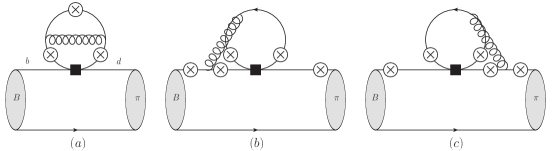
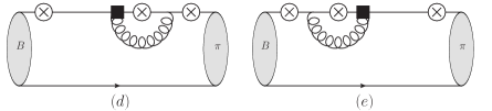
Figure 3: Factorizable NLO quark-loop contributions to $B\to\pi\ell^{+}\ell^{-}$, due to the four-quark effective operators $O_{1,2}^{u,c}$ (upper panel) and the chromomagnetic operator $O_{8g}$ (lower panel). The notation is the same as in Fig. 2.

The NLO corrections to the quark loops generated by the current-current operators $O^{u,c}_{1,2}$ are given by the two-loop diagrams shown in Fig. 3 (a),(b),(c). The contributions of quark-penguin operators are neglected, being suppressed by small Wilson coefficients and $\alpha_{s}$ simultaneously. In the same order of the perturbative expansion, the chromomagnetic operator $O_{8g}$ is described with the diagrams shown in Fig. 3(d),(e). These factorizable NLO contributions were taken into account in QCDF [3, 4], employing the quark-level two-loop diagrams calculated in Ref. [15] (see also Refs. [16, 17]). The NLO contribution of $O_{1,2}^{c}$ to ${\cal H}^{(c)}$ can be literally taken from Ref. [9], replacing $f^{+}_{BK}(q^{2})$ by $f^{+}_{B\pi}(q^{2})$. The corresponding contribution to ${\cal H}^{(u)}$ has the same structure, so that we can present both contribution by one compact expression:

$${\cal H}^{(p)}_{\rm fact,NLO}=-\frac{\alpha_{s}}{32\pi^{3}}\frac{m_{b}}{m_{B}}\Biggl{\{}C_{1}F_{2,p}^{(7)}(q^{2})+C_{8}^{\rm eff}F_{8}^{(7)}(q^{2})$$

$$+\frac{m_{B}}{2m_{b}}\biggl{[}C_{1}F_{2}^{(9)}+2C_{2}\left(F_{1,p}^{(9)}(q^{2})+\frac{1}{6}F_{2,p}^{(9)}(q^{2})\right)+C_{8}^{\rm eff}F_{8}^{(9)}(q^{2})\biggr{]}\Biggr{\}}f^{+}_{B\pi}(q^{2}),$$ (19)

where $p=u,c$. The definitions and nomenclature of the indices of the functions $F^{(7,9)}_{1,p}$, $F^{(7,9)}_{2,p}$ and $F_{8}^{(7,9)}$ are the same as in Refs. [15, 16]. The only difference is that $F_{1,c}^{(7,9)}$ and $F_{2,c}^{(7,9)}$ are expressed as a double expansion in $\hat{s}=q^{2}/m_{b}^{2}$ and $\hat{m}_{c}^{2}=m_{c}^{2}/m_{b}^{2}$, whereas $F_{1,u}^{(7,9)}$ and $F_{2,u}^{(7,9)}$ are expanded only in powers $\hat{s}=q^{2}/m_{b}^{2}$ since we work in the limit $m_{u}=0$. It has been shown in Refs. [15, 16] that keeping the terms up to the third power of $\hat{s}$ and $\hat{m}_{c}^{2}$ provides a sufficient numerical accuracy in the region $0.05\leq\hat{s}\leq 0.25$. Here we use this expansion for $q^{2}<0$, restricting ourselves to $1.0\leq|q^{2}|\leq 4.0$ GeV², i.e. staying within the same region. For $F_{8}^{(7,9)}$ we use the expression derived in Ref. [3].

We remind that at NLO, the nonlocal contributions acquire the imaginary part also at $q^{2}<0$, that is, not related to the singularities in the variable $q^{2}$. The origin of this imaginary part and its relation to the final-state strong interaction is the same as for $B\to K\ell^{+}\ell^{-}$ and is explained in detail in Ref. [9].

Note that analytic expressions for the two-loop virtual corrections to the matrix elements of the $O_{1}^{u}$ and $O_{2}^{u}$ operators are available from Ref. [17]. These expressions are valid at $q^{2}>0$ and agree with the expansion in $q^{2}/m_{b}^{2}$ obtained in Ref. [16]. However, we cannot use the results of Ref. [17] straightforwardly in our calculation at $q^{2}<0$, without separating the imaginary contributions inherent to the negative $q^{2}$-region from the contributions appearing due to the cuts of quark-gluon diagrams at $q^{2}>0$. Hence, we prefer to use the expanded form of these corrections [16] in which the phases stemming from the positivity of $q^{2}$, e.g., the terms proportional to $i\pi$ and originating from the $\log q^{2}$ terms can be easily recognized and separated. As we work at sufficiently small values of $|q^{2}|$, the accuracy of the expansion in Ref. [16] is sufficient.

Contrary to the LO contributions considered in the previous subsections, the factorizable NLO ones are not simply accessible within the LCSR approach. Indeed, in order to reach the same $O(\alpha_{s})$ accuracy, the calculation of the underlying correlation function has to include two-loop diagrams with several scales, a task exceeding the currently reached level of complexity in the multiloop calculations.

3.4 Nonfactorizable soft-gluon contributions

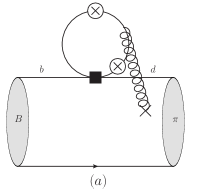
Figure 4: Nonfactorizable soft-gluon contributions to $B\to\pi\ell^{+}\ell^{-}$ due to (a) the four-quark effective operators $O_{1,2}^{u,c}$ and $O_{3-6}$ and (b) the chromomagnetic $O_{8g}$ operator. The soft gluon is represented by the gluon line with a cross. The rest of notation is the same as in the previous figures.

We also take into account the nonfactorizable contributions to the amplitudes ${\cal H}^{(p)}(q^{2})$ emerging due to a soft-gluon emission from the quark loops, as shown in Fig. 4. These hadronic matrix elements cannot be reduced to a $B\to\pi$ form factor. It is also not possible to attribute the soft gluon to one of the hadrons in the $B\to\pi$ transition. The soft-gluon contributions are nevertheless well defined at $q^{2}<0$ and $|q^{2}|\gg\Lambda_{QCD}^{2}$. As shown in Ref. [8], their suppression with respect to the factorizable loops is controlled by the powers of $1/(4m_{c}^{2}-q^{2})$ and $1/|q^{2}|$, stemming, respectively, from the $c$-quark and massless loops with soft gluon. The corresponding hadronic matrix elements were first calculated for the $c$-quark loops in Ref. [8] for $B\to K^{(*)}\ell^{+}\ell^{-}$. The calculation was done in two steps: (1) applying the light-cone OPE at deep spacelike $q^{2}$ for the quark loop with soft-gluon emission, and (2) calculating the $B\to K^{(*)}$ hadronic matrix element of the emerging quark-antiquark-gluon operator using LCSRs with the $B$-meson three-particle DAs. Completing this result to include the loops with all possible quark flavours is straightforward and was already done for $B\to K\ell^{+}\ell^{-}$ in Ref. [9]; to obtain the corresponding contribution to ${\cal H}^{(c)}(q^{2})$ in $B\to\pi\ell^{+}\ell^{-}$, we only need to replace the kaon by the pion. The soft-gluon nonfactorizable contribution of the operator $O_{1}^{u}$ contributing to ${\cal H}^{(u)}(q^{2})$, is also easily obtained. The result for this contribution is cast in a compact form:

$${\cal H}^{(p)}_{\rm soft}(q^{2}) = \frac{4}{3}\left(\delta_{pc}C_{1}+C_{4}-C_{6}\right)\tilde{A}(m_{c}^{2},q^{2})+\frac{2}{3}\left(2\delta_{pu}C_{1}+C_{4}-C_{6}\right)\tilde{A}(0,q^{2})$$ (20)

$$- \frac{2}{3}\left(C_{3}+C_{4}-C_{6}\right)\left(\tilde{A}(m_{s}^{2},q^{2})+\tilde{A}(m_{b}^{2},q^{2})\right)\,.$$

A cumbersome expression for the nonfactorizable hadronic matrix element $\tilde{A}(m_{q}^{2},q^{2})$ obtained from LCSR can be found in Ref. [8],(see Eq. (4.8) therein), where the dependence on the quark mass squared is explicitly shown and is indicated in the above expression. To adjust this expression to the $B\to\pi\ell^{+}\ell^{-}$ transition, one has to replace the decay constant, meson mass and threshold parameter in this equation: $f_{K}\to f_{\pi}$, $m_{K}\to m_{\pi}$, $s_{0}^{K}\to s_{0}^{\pi}$, thus taking into account the flavour $SU(3)$ violation. In the sum rule for $\tilde{A}(m_{q}^{2},q^{2})$, we use the ansatz for the three-particle $B$-meson DAs suggested in Ref. [23], with the parameter $\lambda_{E}^{2}=3/2\lambda_{B}^{2}$, directly related to the inverse moment of the two-particle DA $\phi^{+}_{B}$ specified in Eq. (17).

The soft-gluon contribution of the chromomagnetic operator $O_{8g}$ is described by the diagram in Fig. 4b, where instead of the loop factor, one has a pointlike emission of the soft gluon field. One modifies the correlation function accordingly and arrives at the LCSR that was already derived in Ref. [9] and presented in Eq. (4.7) therein. Making the necessary replacements for $B\to\pi\ell^{+}\ell^{-}$, we obtain

$${\cal H}_{\rm soft,O_{8g}}^{(u)}(q^{2})={\cal H}_{\rm soft,O_{8g}}^{(c)}(q^{2})=\Big{[}{\cal H}^{(BK)}_{\rm soft,O_{8g}}(q^{2})\Big{]}_{f_{K}\to f_{\pi}\,,m_{K}\to m_{\pi},\,s_{0}^{K}\to s_{0}^{\pi}}\,.$$ (21)

As in the case of $B\to K\ell^{+}\ell^{-}$ transitions, this contribution turns out to be very small.

3.5 Nonfactorizable spectator scattering

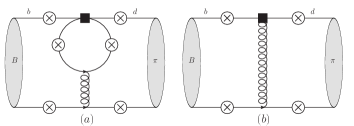
Figure 5: Nonfactorizable spectator contributions to $B\to\pi\ell^{+}\ell^{-}$ due to (a) the four-quark effective operators $O_{1,2}^{u,c}$, $O_{3-6}$ and (b) the chromomagnetic operator $O_{8g}$.

An important nonlocal contribution to the $B\to\pi\ell^{+}\ell^{-}$ amplitude in NLO emerges due to a hard gluon emitted from the intermediate quark loop or from the $O_{8g}$-operator vertex, and absorbed by the spectator quark in the $B\to\pi$ transition, as shown in Fig. 5. Following [9], we will use the QCDF result [3] for this contribution. The following expression is valid for both $p=u$ and $p=c$ parts of the nonlocal amplitude:

$${\cal H}^{(p)}_{\rm nonf,spect}(q^{2}) = \frac{\alpha_{s}C_{F}}{32\pi N_{c}}\frac{f_{B}f_{\pi}m_{b}}{m_{B}^{2}}\Biggl{(}\int\limits_{0}^{\infty}\frac{d\omega}{\omega}\phi_{B}^{+}(\omega)\int\limits_{0}^{1}du\,\varphi_{\pi}(u)\,T_{+}^{(1),p}(u,\omega)+$$ (22)

$$+ \int\limits_{0}^{\infty}\frac{d\omega}{\omega}\phi_{B}^{-}(\omega)\int\limits_{0}^{1}du\,\varphi_{\pi}(u)\,T_{-}^{(1),p}(u,\omega)\Biggl{)}\,.$$

The hard-scattering kernels entering the above expression have the form:

$$T_{+}^{(1),p}(u,\omega) = -\frac{m_{B}}{m_{b}}\Biggl{(}\frac{2}{3}t_{\parallel}(u,m_{c})(\delta_{pc}C_{1}+C_{4}-C_{6})-\frac{1}{3}t_{\parallel}(u,m_{b})(C_{3}+C_{4}-C_{6})-$$ (23)

$$-\frac{1}{3}t_{\parallel}(u,m_{s})(C_{3}+C_{4}-C_{6})+\frac{1}{3}(2\delta_{pu}C_{1}+C_{4}-C_{6})t_{\parallel}(u,0)\Biggl{)},$$

$$T_{-}^{(1),p}(u,\omega) = -Q_{q}\frac{m_{B}\omega}{m_{B}\omega-q^{2}-i\epsilon}\Biggl{[}\frac{8m_{B}}{3m_{b}}\biggl{(}h(m_{c}^{2},\bar{u}m_{B}^{2}+uq^{2})(\delta_{pc}C_{1}+C_{4}+C_{6})+$$ (24)

$$+h(m_{b}^{2},\bar{u}m_{B}^{2}+uq^{2})(C_{3}+C_{4}+C_{6})+$$

$$+h(0,\bar{u}m_{B}^{2}+uq^{2})(\delta_{pu}C_{1}+C_{3}+3C_{4}+3C_{6})-$$

$$-\frac{2}{3}(C_{3}-C_{5}-15C_{6})\biggr{)}+\frac{8C_{8}^{\rm eff}}{\bar{u}+uq^{2}/m_{B}^{2}}\Biggr{]},$$

where $Q_{q}$ is the electric charge of the spectator quark in the $B$-meson ($q=u,d$) and the functions $t_{\parallel}(u,m_{q})$ and $h(m_{q}^{2},q^{2})$ can be found in Ref. [3].

The two-particle $B$-meson DAs $\phi_{B}^{\pm}(\omega)$ are given in Eq.(17); for the twist-2 pion DA we employ the standard Gegenbauer expansion:

$$\varphi_{\pi}(u,\mu)=6u(1-u)\Big{(}1+a_{2}^{\pi}(\mu)C_{2}^{(3/2)}(u)+a_{4}^{\pi}(\mu)C_{4}^{(3/2)}(u)\Big{)}\,.$$ (25)

The fact that the amplitudes in (22) depend on the charge of the spectator quark in the $B$ meson triggers another important contribution to the isospin asymmetry in $B\to\pi\ell^{+}\ell^{-}$.

Summing up all contributions considered in this section, we obtain the two nonlocal amplitudes in the adopted approximation:

$${\cal H}^{(p)}(q^{2}) = {\cal H}^{(p)}_{\rm fact,LO}(q^{2})+{\cal H}^{(p)}_{\rm WA}(q^{2})+{\cal H}^{(p)}_{\rm fact,NLO}(q^{2})$$ (26)

$$+ {\cal H}^{(p)}_{\rm soft}(q^{2})+{\cal H}^{(p)}_{\rm soft,O_{8}}(q^{2})+{\cal H}^{(p)}_{\rm nonf,spect}(q^{2})\,,\qquad(p=u,c)\,.$$

4 Numerical analysis

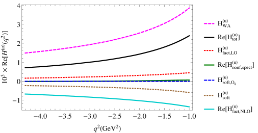
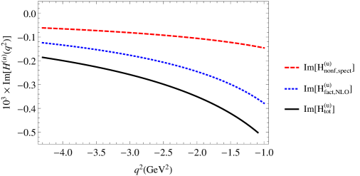
Figure 6: Nonlocal amplitude ${\cal H}^{(u)}(q^{2})$ for $B^{-}\to\pi^{-}\ell^{+}\ell^{-}$ at $q^{2}<0$ calculated at the central values of the input; the real (imaginary) part is in the upper (lower) panel; $H^{(u)}_{\rm tot}(q^{2})$ is the sum of the separate contributions specified in Eq.(26).

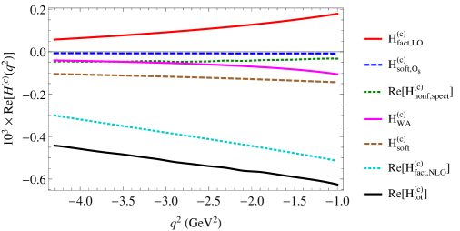
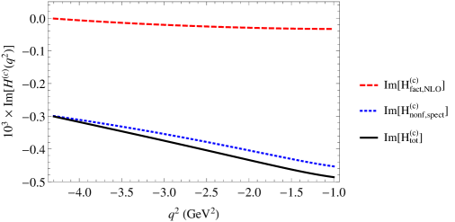
Figure 7: The same as in Fig.6 for the amplitude ${\cal H}^{(c)}(q^{2})$ for $B^{-}\to\pi^{-}\ell^{+}\ell^{-}$.

Here we perform the numerical analysis of the nonlocal amplitudes (26) at spacelike $q^{2}<0$, more definitely, in the region $1\,\mbox{ GeV}^{2}\leq|q^{2}|\lesssim 4\,\mbox{ GeV}^{2}$, where the OPE and QCDF approximation can be trusted. The input parameters and references to their source are listed in Table 1, the charged and neutral $B$-meson and pion masses are taken from [18], and the numerical values of the Wilson coefficients are presented in the Appendix A.

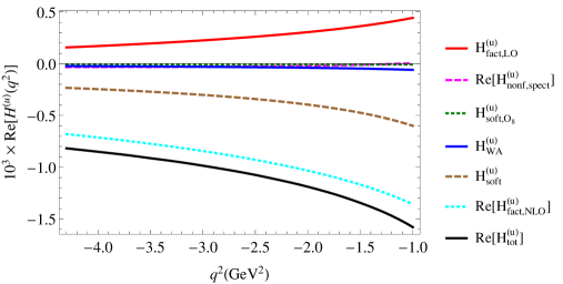
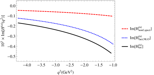
Figure 8: The same as in Fig.6 for the amplitude ${\cal H}^{(u)}(q^{2})$ in $\bar{B}^{0}\to\pi^{0}\ell^{+}\ell^{-}$.

Input parameter	[Ref.]
$\alpha_{s}(m_{Z})=0.1185\pm 0.0006$
$\overline{m}_{c}(\overline{m}_{c})=(1.275\pm 0.025)$ GeV
$\overline{m}_{b}(\overline{m}_{b})=(4.18\pm 0.03)$ GeV	}[18]
$m_{s}(2{\rm GeV})=(95\pm 5)$ MeV
$f_{B}=207^{+17}_{-9}$ MeV	[20]
$\lambda_{B}=(460\pm 110)$ MeV	[21]
$f_{\pi}=130.4$ MeV	[18]
$a_{2}^{\pi}(1{\rm GeV})=0.17\pm 0.08$
$a_{4}^{\pi}(1{\rm GeV})=0.06\pm 0.10$	[22]
Sum rules in the pion channel
$M^{2}=1.0\pm 0.5$ GeV2 ,  $s_{0}^{\pi}=0.7$ GeV2	[23]
$f^{+}_{B\pi}(0)=0.307\pm 0.020$
$b_{1}^{+}=-1.31\pm 0.42$	}[19]
$b_{2}^{+}=-0.904\pm 0.444$

Table 1: Intervals of the input parameters used in the calculation of ${\cal H}^{(u,c)}(q^{2}<0)$.

As a default renormalization and factorization scale we assume $\mu=3$ GeV, the same as in Ref. [9]. It will be varied in the interval $2.5<\mu<4.5$ GeV to study the $\mu$ dependence.

For the vector $B\to\pi$ form factor the most recent update [19] of LCSR prediction is adopted, in a form fitted to the three-parameter BCL parameterization:

$$f^{+}_{B\pi}(q^{2})=\frac{f^{+}_{B\pi}(0)}{1-q^{2}/m_{B^{*}}^{2}}\Bigg{\{}1+b_{1}^{+}\Bigg{[}z(q^{2},t_{0})-z(0,t_{0})-\frac{1}{3}\Big{(}z(q^{2},t_{0})^{3}-z(0,t_{0})^{3}\Big{)}\Bigg{]}$$

$$+b_{2}^{+}\Bigg{[}z(q^{2},t_{0})^{2}-z(0,t_{0})^{2}+\frac{2}{3}\Big{(}z(q^{2},t_{0})^{3}-z(0,t_{0})^{3}\Big{)}\Bigg{]}\Bigg{\}}$$ (27)

with $t_{0}=(m_{B}+m_{\pi})(\sqrt{m_{B}}-\sqrt{m_{\pi}})^{2}$, where the normalization and shape parameters are presented in Table 1. The decay constant of $B$ meson is determined from two-point sum rules, where we use the recent analysis [20]; the inverse moment of the $B$-meson DA is also represented by the interval of QCD sum rule prediction [21]. The intervals of Gegenbauer moments in the pion DAs used in the QCDF expressions are the same as in the LCSR for the $B\to\pi$ form factor [19, 22].

Substituting the central input in the expressions presented in the previous section, we calculate the two amplitudes ${\cal H}^{(u)}(q^{2}<0)$ and ${\cal H}^{(c)}(q^{2}<0)$ for $B^{-}\to\pi^{-}\ell^{+}\ell^{-}$ and plot their real and imaginary parts in Figs. 6 and 7, respectively, showing also the separate contributions. For comparison, the amplitude ${\cal H}^{(u)}(q^{2}<0)$ is plotted in Fig. 8 for $\bar{B}^{0}\to\pi^{0}\ell^{+}\ell^{-}$, whereas the amplitude ${\cal H}^{(c)}(q^{2}<0)$ for the latter mode is numerically similar to the one for $B^{-}\to\pi^{-}\ell^{+}\ell^{-}$ and is not shown.

From the numerical analysis we can draw several conclusions:

(a) The contributions to ${\cal H}^{(c)}(q^{2})$ are approximately the same as the corresponding ones for the $B\to K\ell^{+}\ell^{-}$ obtained in Ref. [9], the differences reflect the violation of the flavour $SU(3)$ symmetry;

(b) The contributions to ${\cal H}^{(u)}(q^{2})$, in $B^{-}\to\pi^{-}\ell^{+}\ell^{-}$ presented in Fig. 6 are clearly dominated by the weak annihilation term, enhancing the real part of ${\cal H}^{(u)}(q^{2})$ considerably. This effect is less pronounced for $\bar{B}^{0}\to\pi^{-}\ell^{+}\ell^{-}$, as expected;

(c) The nonfactorizable soft-gluon contribution due to the operators $O_{1,2}^{u,c}$ are important and the corresponding contributions of $O_{3-6}$ are not negligible. Meanwhile, the contribution due to the operator $O_{8g}$ with a soft-gluon is very small.

The uncertainties of the functions ${\cal H}^{(c)}(q^{2}<0)$ and ${\cal H}^{(u)}(q^{2}<0)$ are estimated varying the inputs within their adopted intervals indicated in Table 1. The largest uncertainties originate from the variation of $f_{B}$, $\lambda_{B}$ and the correlated variation of the parameters of $f_{B\pi}^{+}$. To stay on the conservative side, we neglect possible correlations between the individual input entries in Table 1. We also varied the renormalization/factorization scale around the default “optimal” value $\mu=3.0$ GeV. The results do not significantly change the estimated total uncertainty and we therefore neglect the scale dependence in the error estimates performed below.

5 Nonleptonic $B\to V\pi$ decay amplitudes

We now turn to weak nonleptonic $B\to V\pi$ decays with neutral vector mesons $V=\rho^{0},\omega,\phi,J/\psi,\psi(2S)$ in the final state. The intervals of the absolute values of their amplitudes have to be estimated and used as an input in the hadronic dispersion relations for ${\cal H}^{(u,c)}(q^{2})$ to be fitted to the calculated ${\cal H}^{(u,c)}(q^{2}<0)$.

The amplitude of a $B^{-}\to V\pi^{-}$ decay is parametrized as:

$$A(B^{-}\to V\pi^{-}) = \langle V(q)\pi^{-}(p)|H_{\rm eff(NL)}^{b\to d}|B^{-}(p+q)\rangle$$ (28)

$$= \frac{4G_{F}}{\sqrt{2}}m_{V}(\varepsilon_{V}^{*}\cdot p)\bigg{(}\lambda_{u}A_{B^{-}V\pi^{-}}^{u}+\lambda_{c}A_{B^{-}V\pi^{-}}^{c}\bigg{)}\,,$$

where $q$ ($\varepsilon_{V}$) is the 4-momentum (polarization vector) of the vector meson with $q^{2}=m_{V}^{2}$. For the charge-conjugated mode $B^{+}\to V\pi^{+}$ one has to replace $\lambda_{u,c}\to\lambda_{u,c}^{*}$ in the above relation, whereas the hadronic amplitudes remain unchanged, $A_{B^{-}V\pi^{-}}^{u,c}=A_{B^{+}V\pi^{+}}^{u,c}$. For the neutral $\bar{B}^{0}\to V\pi^{0}$ decay modes we denote the corresponding amplitudes as $A_{\bar{B}^{0}V\pi^{0}}^{u,c}=A_{B^{0}V\pi^{0}}^{u,c}$. The effective Hamiltonian $H_{\rm eff(NL)}^{b\to d}$ in Eq. (28) contains the operators $O_{1,2}^{u,c}$, $O_{3-6}$, $O_{8g}$ given in Appendix A, and we neglect the electroweak quark-penguin operators with $O(\alpha_{\rm em})$ suppressed Wilson coefficients. From Eq. (28) one obtains the expression for the $CP$-averaged width:

$$\Gamma(B^{\mp}\to V\pi^{\mp})\equiv\frac{1}{2}\big{[}\Gamma(B^{-}\to V\pi^{-})+\Gamma(B^{+}\to V\pi^{+})\big{]}=\frac{G_{F}^{2}\lambda^{3/2}(m_{B}^{2},m_{\pi}^{2},m_{V}^{2})}{8\pi m_{B}^{3}}$$

$$\times\bigg{(}|\lambda_{u}|^{2}|A_{B^{-}V\pi^{-}}^{u}|^{2}+|\lambda_{c}|^{2}|A_{B^{-}V\pi^{-}}^{c}|^{2}+2|\lambda_{u}\lambda_{c}||A_{B^{-}V\pi^{-}}^{u}||A_{B^{-}V\pi^{-}}^{c}|\cos\delta\cos\Delta\bigg{)}\,,$$ (29)

where $\lambda(a,b,c)=a^{2}+b^{2}+c^{2}-2ab-2ac-2bc$. In the above, we explicitly isolate the relative strong phase $\delta$ between the amplitudes $A_{B^{-}V\pi^{-}}^{u}$ and $A_{B^{-}V\pi^{-}}^{c}$ and denote $\Delta\equiv{\rm arg}(\lambda_{u})-{\rm arg}(\lambda_{c})$. The direct $CP$ asymmetry takes the following form:

$${\cal A}_{CP}(B^{\mp}\to V\pi^{\mp})\equiv\frac{\Gamma(B^{-}\to V\pi^{-})-\Gamma(B^{+}\to V\pi^{+})}{2\Gamma(B^{\mp}\to V\pi^{\pm})}$$

$$=-2\sin{\delta}\sin\Delta\bigg{(}\left|\frac{\lambda_{u}A^{u}_{B^{-}V\pi^{-}}}{\lambda_{c}A^{c}_{B^{-}V\pi^{-}}}\right|+\left|\frac{\lambda_{c}A^{c}_{B^{-}V\pi^{-}}}{\lambda_{u}A^{u}_{B^{-}V\pi^{-}}}\right|+2\cos\delta\cos\Delta\bigg{)}^{-1}\,.$$ (30)

Analogous expressions are obtained for the neutral $B\to V\pi^{0}$ modes, replacing $B^{-}\to\bar{B}^{0}$ and $B^{+}\to B^{0}$.

For the input in the two dispersion relations for the amplitudes ${\cal H}^{(u)}(q^{2})$ and ${\cal H}^{(c)}(q^{2})$ we need to separately determine the moduli of the hadronic amplitudes $|A_{B^{-}V\pi^{-}}^{u}|$ and $|A_{B^{-}V\pi^{-}}^{c}|$. In principle, one can use the two observables in Eqs (28) and (30), but the presence of the third unknown parameter, the relative strong phase, hinders the determination. Therefore, the situation is more complex here than for the nonleptonic $B\to VK$ decays used in the analysis of $B\to K\ell^{+}\ell^{-}$ in Ref. [9] where only the contributions proportional to $\lambda_{c}$ were retained and the amplitudes $|A_{BVK}^{c}|$ were directly obtained from the measured $B\to VK$ branching fractions.

On the other hand, there is a possibility to estimate separate contributions to the nonleptonic amplitudes applying the QCDF approach [2]. The latter is known to provide a reasonably good description of the charmless channels $B^{-}\to\rho^{0}\pi^{-}$ and $B^{-}\to\omega^{0}\pi^{-}$. Here we use the results of Ref. [10] where the QCDF description for $B\to VP$ decays was elaborated in detail. The necessary expressions for the amplitude decomposition and the additional input parameters including the $B\to V$ form factors, decay constants and the Gegenbauer moments of the DAs of $V=\rho,\omega$ are collected in Appendix B. The resulting absolute values of the amplitudes are presented in Table 2. To check the validity of these estimates, we calculated the observables (28) and (30), and compared the results with the experiment and with the earlier predictions of Ref. [10] (see Table 3), observing a reasonable agreement. In the transition from the widths to branching fractions we use the lifetimes of $B$ mesons from Ref. [18].

Mode	$|A_{BV\pi}^{u}|$	$|A_{BV\pi}^{c}|$
$B^{\mp}\to\rho^{0}\pi^{\mp}$	$20.8^{+2.7}_{-2.3}$	$1.3^{+1.1}_{-0.4}$
$B^{\mp}\to\omega\pi^{\mp}$	$19.1^{+2.7}_{-2.0}$	$0.3^{+0.4}_{-0.1}$
$B^{\mp}\to J/\psi\pi^{\mp}$	$0.5^{+9.7}_{-0.5}$	$29.2^{+1.4}_{-1.5}$
$B^{\mp}\to\psi(2S)\pi^{\mp}$	$3.5^{+6.7}_{-3.5}$	$32.3^{+2.0}_{-2.1}$

Mode	$|A_{BV\pi}^{u}|$	$|A_{BV\pi}^{c}|$
$B^{0}\to\rho^{0}\pi^{0}$	$9.9^{+1.3}_{-1.4}$	$0$
$B^{0}\to\omega\pi^{0}$	$0$	$0$
$B^{0}\to J/\psi\pi^{0}$	$0.3^{+6.9}_{-0.3}$	$20.6^{+1.0}_{-1.1}$
$B^{0}\to\psi(2S)\pi^{0}$	$2.4^{+4.7}_{-2.4}$	$22.8^{+1.4}_{-1.5}$

Table 2: Inputs for the absolute values $|A_{BV\pi}^{u,c}|$ of the $B\to V\pi$ amplitudes (in MeV).

Note that in the dispersion relations we will not isolate the intermediate $\phi$-meson pole, hence we do not specify the $B\to\phi\pi$ nonleptonic amplitudes here. These decays originate either due to the $q=s$ part of the quark-penguin operators $O_{3-6}$ with suppressed Wilson coefficients, or due to the $O_{1,2}$ operators combined with a transition via intermediate gluons into $\bar{s}s$ state. The latter is OZI suppressed (cf. the smallness of $\phi$ decays into pions). The measured upper limit ${\rm BR}(B^{-}\to\phi\pi^{-})<1.5\times 10^{-7}$ [18], being significantly smaller than the measured branching fractions of $B^{-}\to\rho(\omega)\pi^{-}$ decays (see Table 3) convinces us that the intermediate $\phi$-meson contribution to $B\to\pi\ell^{+}\ell^{-}$ is small. Furthermore we do not separate the radial excitations $\rho^{\prime},...,\omega^{\prime},...$, approximating their contributions to the hadronic spectral density by the quark-hadron duality ansatz; hence we do not need to consider here the nonleptonic decays of the type $B\to\rho^{\prime}(1450)\pi$.

Channel	Observable	Experiment	QCDF [10]	QCDF, this work
$B^{\pm}\to\rho^{0}\pi^{\pm}$	${\rm BR}\times 10^{6}$	$8.3\pm 1.2$	$11.9^{+7.8}_{-6.1}$	$9.5^{+2.9}_{-1.8}$
	${\cal A}_{CP}$	$0.18^{+0.09}_{-0.17}$	$\phantom{-}0.04\pm 0.19$	$0.09\pm 0.17$
$B^{\pm}\to\omega^{0}\pi^{\pm}$	${\rm BR}\times 10^{6}$	$6.9\pm 0.5$	$8.8^{+5.4}_{-4.3}$	$8.9^{+2.6}_{-1.6}$
	${\cal A}_{CP}$	$-0.04\pm 0.06$	$-0.02\pm 0.04$	$-0.06\pm 0.06$
$B^{0}\to\rho^{0}\pi^{0}$	${\rm BR}\times 10^{6}$	$2.0\pm 0.5$	$0.4^{+1.1}_{-0.4}$	$0.2^{+0.4}_{-0.1}$
	${\cal A}_{CP}$	—	$-0.16^{+0.26}_{-0.32}$	$0.24^{+0.36}_{-0.31}$
$B^{0}\to\omega^{0}\pi^{0}$	${\rm BR}\times 10^{6}$	$<0.5$	$0.01^{+0.04}_{-0.01}$	$0.01^{+0.06}_{-0.01}$
	${\cal A}_{CP}$	—	—	$-0.94^{+0.87}_{-0.04}$

Table 3: Comparison of the experimental data [18] and theoretical predictions for the observables in the nonleptonic $B\to\rho(\omega)\pi$ decays.

For the neutral $B^{0}\to V\pi^{0}$ modes, the QCDF prediction [10] fails to predict the partial width $B^{0}\to\rho^{0}\pi^{0}$, the experimental value being significantly larger. Without going into more detailed discussion of this problem, guided by the hierarchy of amplitudes in the charged mode, $A_{B^{0}\rho^{0}\pi^{0}}^{c}\ll A_{B^{0}\rho^{0}\pi^{0}}^{u}$, we simply assume $A_{B^{0}\rho^{0}\pi^{0}}^{c}=0$ and extract $|A_{B^{0}\rho^{0}\pi^{0}}^{u}|$ from the measured partial width employing Eq. (29). For the $B^{0}\to\omega\pi^{0}$ mode only the upper limit on the branching fraction is available [18], indicating that this decay amplitude is suppressed in comparison to the other modes, hence we put $A_{B^{0}\omega\pi^{0}}^{u}\approx A_{B^{0}\omega\pi^{0}}^{c}\approx 0$ as it specified in Table 2.

Turning to the charmonium channels $B\to\psi\pi$, where $\psi=J/\psi,\psi(2S)$, we do not expect the QCDF approach to work there due to a heavy final state and enhanced nonfactorizable, power suppressed effects (see, e.g., the discussion in Ref. [8]). On the other hand, one anticipates that these nonleptonic decays are dominated by the emission topology due to the operators $O_{1,2}^{c}$ with large Wilson coefficients and a small admixture of $O_{3-6}$ ($q=c$). The contributions of the operators $O_{1,2}^{u}$ and $O_{3-6}$ $(q\neq c)$ are expected to be strongly suppressed. Theoretical estimates for the analogous contributions to $B\to\psi K$ transitions (see, e.g., [24] and [25]) yield the amplitudes of gluonic transitions of light-quark loops to charmonium states at the level of $10^{-3}$ of the dominant contributions of $O_{1,2}^{c}$ operators. With an extra Cabibbo enhancement of the $\lambda_{u}$ terms in $B\to\psi\pi$ with respect to $B\to\psi K$, still a considerable suppression remains. Hence we expect that $|A_{B^{-}\psi\pi^{-}}^{u}|\ll|A_{B^{-}\psi\pi^{-}}^{c}|$. In this situation the relative strong phase does not considerably influence the extraction of the large $\sim\lambda_{c}$ term , whereas the uncertainty of the small $\sim\lambda_{u}$ term is tolerable. Therefore, we use the current experimental data on the branching fractions and $CP$-asymmetries of the above decays [18] and perform the fit of these data to the Eqs. (29) and (30), extracting the absolute values of the amplitudes $|A_{B^{-}\psi\pi^{-}}^{u}|$ and $|A_{B^{-}\psi\pi^{-}}^{u}|$ and allowing the relative phase $\delta$ to change from 0 to $2\pi$. The resulting intervals are presented in Table  2. Finally, for the neutral $\bar{B}^{0}\to\psi\pi^{0}$ modes, we make use of the isospin symmetry relation: $A_{B^{0}\psi\pi^{0}}^{u,c}\simeq 1/\sqrt{2}A_{B^{-}\psi\pi^{-}}^{u,c}$, since for the dominant $\psi$ emission mechanism of these decays there is only one independent isospin amplitude. This assumption is supported by the measurement [18] yielding $\Gamma(B^{0}\to J/\psi\pi^{0})\simeq 1/2\Gamma(B^{+}\to J/\psi\pi^{+})$ . The resulting estimates are also presented in Table 2.

6 Hadronic dispersion relations

Following Refs.[8, 9], the invariant amplitudes ${\cal H}^{(u)}(q^{2})$ and ${\cal H}^{(c)}(q^{2})$ are represented in a form of hadronic dispersion relations in the variable $q^{2}$, inserting the total set of hadronic intermediate states between the electromagnetic current and the effective operators in the correlation functions (2):

$${\cal H}^{(p)}(q^{2})-{\cal H}^{(p)}(q_{0}^{2}) = (q^{2}-q^{2}_{0})\Biggr{[}\sum\limits_{V=\rho,\omega,J/\psi,\psi(2S)}\frac{k_{V}f_{V}A_{BV\pi}^{p}}{(m_{V}^{2}-q_{0}^{2})(m_{V}^{2}-q^{2}-im_{V}\Gamma_{V}^{\rm tot})}$$ (31)

$$+\int\limits_{s_{h}}^{\infty}ds\frac{\rho_{h}^{(p)}(s)}{(s-q_{0}^{2})(s-q^{2}-i\epsilon)}\Biggl{]}\,,\quad(p=u,c)\,,$$

where the ground-state vector mesons (except $\phi$) are isolated and the integral describes the contribution of excited and continuum contributions starting from $s_{h}=4m_{\pi}^{2}$, the lowest hadronic threshold . To achieve a better convergence, we implement one subtraction at $q_{0}^{2}=-1.0$ GeV² in Eq. (31). In the above, the masses and total widths of the vector mesons $V=\rho^{0},\omega,J/\psi,\psi(2S)$ are taken from Ref. [18]. Their decay constants are defined as

$$\langle 0|j^{{\rm em},\,\mu}|V(q)\rangle=k_{V}m_{V}\varepsilon_{V}^{\mu}(q)f_{V}\,,$$ (32)

where the coefficients $k_{V}$ are determined by the valence-quark content of $V$ and the quark charges: $k_{\rho}=1/\sqrt{2}$, $k_{\omega}=1/(3\sqrt{2})$ and $k_{J/\psi}=k_{\psi(2S)}=2/3$. The numerical values of $f_{V}$ are fixed from the measured [18] leptonic widths $\Gamma(V\to\ell^{+}\ell^{-})$ yielding $f_{\rho}=221$ MeV, $f_{\omega}=195$ MeV, $f_{J/\psi}=416$ MeV and $f_{\psi(2S)}=297$ MeV. The absolute values of the amplitudes $A_{BV\pi}^{u}$ and $A_{BV\pi}^{c}$ obtained from the analysis of nonleptonic decays in the previous section are taken from Table 2.

At $q^{2}<0$, more specifically, in the region $-4.0\leavevmode\nobreak\ \mbox{GeV}^{2}\leq q^{2}\leq-1.0\leavevmode\nobreak\ \mbox{GeV}^{2}$, we substitute in the l.h.s of the relations (31) the result for $H^{(p)}(q^{2})$ specified in Eq. (26), calculating simultaneously the subtraction terms at $q_{0}^{2}=-1.0\leavevmode\nobreak\ \mbox{GeV}^{2}$. The task is then to fit the free parameters on the r.h.s. of the hadronic dispersion relations. Importantly, each $V$-pole residue in Eq. (31) for $p=u$ or $p=c$ has a relative phase with respect to the other vector-meson contributions and to the integral over $\rho^{(p)}_{h}(s)$. These phases should match the imaginary part of the calculated l.h.s. of the dispersion relation. As explained in Ref. [9], the phases emerge due to the intermediate on-shell hadronic states in the variable $(p+q)^{2}=m_{B}^{2}$ and are not related to the analytical continuation in the variable $q^{2}$.

Note that the relative strong phase between the amplitudes $A_{BV\pi}^{u}$ and $A_{BV\pi}^{c}$ contributing to the $B\to V\pi$ nonleptonic amplitude, although of the same origin, is a different quantity, because in each of dispersion relations (31) only one of these amplitudes enter. On the other hand, calculating the phases of nonleptonic amplitudes within a theoretical framework, such as QCDF, it is possible to estimate the relative phase between, say, $A_{B\rho\pi}^{u}$ and $A_{B\omega\pi}^{u}$.

In what follows, we attribute a phase to each $V$ -pole term:

$$A_{BV\pi}^{p}=|A_{BV\pi}^{p}|\exp(i\delta_{BV\pi}^{(p)})\,.$$ (33)

To reduce the number of free parameters, we fix the phase differences:

$$\delta_{B^{-}\rho^{0}\pi^{-}}^{(u)}-\delta_{B^{-}\omega\pi^{-}}^{(u)}=0.033,\leavevmode\nobreak\ \leavevmode\nobreak\ \delta_{B^{-}\rho^{0}\pi^{-}}^{(c)}-\delta_{B^{-}\omega\pi^{-}}^{(c)}=-3.65,$$ (34)

calculating it from QCDF, as explained in the previous section. Note that for the neutral mode the contribution of the $\omega$-meson is neglected and the corresponding difference is irrelevant. The three remaining phases $\delta_{\rho}^{(p)}$, $\delta_{J/\psi}^{(p)}$ and $\delta_{\psi(2S)}^{(p)}$ for each $p=u,c$ are included into the set of fit parameters. This set will be completed below by the fit parameters of the integrals over $\rho_{h}^{(p)}(s)$. Furthermore, we adopt the Breit-Wigner form of the vector meson contributions in (31) with an energy-dependent total width for the broad $\rho$-resonance so that it vanishes at $q^{2}<4m_{\pi}^{2}$ and adopting constant total widths $\Gamma_{V}^{\rm tot}$ for the remaining narrow resonances.

To complete the ansatz for the hadronic dispersion relations, we have to specify the integrals over the hadronic spectral densities of excited and continuum states $\rho^{(u,c)}(s)$ in Eq.(31). In the region below the open charm threshold, $q^{2}=s\leq 4m_{D}^{2}$, apart from the two narrow charmonium resonances $J/\psi$ and $\psi(2S)$, only the intermediate states with light quark-antiquark flavour content and spin-parity $1^{-}$ contribute. We make extensive use of the standard quark-hadron duality ansatz employed in the QCD sum rules [27] for the vector-meson channels. The integral over the hadronic spectral density $\rho_{h}^{(p)}(s)$ including $\rho^{\prime},\omega^{\prime},...$ and continuum states with the $\rho$ and $\omega$ quantum numbers is replaced by the spectral density calculated from OPE:

$$\rho^{(p)}_{h}(s)\theta(s-s_{h}) \simeq \frac{1}{\pi}\left({\rm Im}{\cal H}_{\rm fact,LO\{u,d\}}^{(p)}(s)+{\rm Im}{\cal H}_{\rm WA}^{(p)}(s)\right)\theta(s-s_{0})$$ (35)

$$+ \frac{1}{\pi}{\rm Im}{\cal H}_{\rm fact,LO\{s\}}^{(p)}(s)\theta(s-\tilde{s_{0}})\,,\leavevmode\nobreak\ \leavevmode\nobreak\ \leavevmode\nobreak\ (p=u,c;\leavevmode\nobreak\ s<4m_{D}^{2})\,,$$

where only the LO contributions are taken into account, including the leading-order quark loops and weak annihilation diagrams. The indices $\{u,d\}$ and $\{s\}$ mean that only the diagrams with $u,d$ and $s$ quarks, respectively, are taken into account. The duality threshold $s_{0}\simeq 1.5$ GeV² is chosen in accordance with the analysis of QCD sum rules in the light vector-meson channels. In the contribution of the intermediate $\bar{s}s$ hadronic states to the spectral density $\rho^{(p)}_{h}(s)$ (the last term in (35)) we include also the small $\phi$-meson pole contribution. This is reflected by the choice of a lower effective threshold parameter $\tilde{s}_{0}=4m_{K}^{2}\simeq 1.0$ GeV². Taking at $s=(q^{2}+i\epsilon)$ the imaginary parts of the loop function (12):

$$\frac{1}{\pi}{\rm Im}\,g(q^{2}+i\epsilon,m_{q}^{2})=\left(1+\frac{2m_{q}^{2}}{q^{2}}\right)\sqrt{1-\frac{4m_{q}^{2}}{q^{2}}}\,\theta(q^{2}-4m_{q}^{2})$$ (36)

and of the WA contribution (18):

$$\frac{1}{\pi}{\rm Im}{\cal H}_{\rm WA}^{(p)}(q^{2}+i\epsilon)=\frac{Q_{q}f_{B}f_{\pi}}{2N_{c}\lambda_{B}m_{B}}e^{-q^{2}/(\lambda_{B}m_{B})}\tilde{C}_{\rm WA}^{p}\theta(s)\,,$$ (37)

we obtain

$$\rho^{(u)}_{LO}(s) = \theta(s-s_{0})\biggl{[}\frac{1}{24\pi^{2}}\left(\frac{2}{3}C_{1}+2C_{2}+C_{3}+\frac{C_{4}}{3}+C_{5}+\frac{C_{6}}{3}\right)f^{+}_{B\pi}(s)+$$ (38)

$$+ Q_{q}\frac{f_{B}f_{\pi}}{2N_{c}\lambda_{B}m_{B}}e^{-s/(\lambda_{B}m_{B})}\left(\delta_{qu}(C_{2}+3C_{1})+\delta_{qd}(C_{1}+3C_{2})+C_{3}+3C_{4}\right)\biggl{]}$$

$$- \frac{1}{24\pi^{3}}\left(\frac{4}{3}C_{3}+\frac{4}{3}C_{4}+C_{5}+\frac{C_{6}}{3}\right){\rm Im}\,g(s,m_{s}^{2})f^{+}_{B\pi}(s)\theta(s-\tilde{s}_{0})$$

and a similar expression:

$$\rho^{(c)}_{LO}(s) = \biggl{[}\frac{1}{24\pi^{2}}\left(C_{3}+\frac{C_{4}}{3}+C_{5}+\frac{C_{6}}{3}\right)f^{+}_{B\pi}(s)+$$ (39)

$$+ Q_{q}\frac{f_{B}f_{\pi}}{2N_{c}\lambda_{B}m_{B}}e^{-s/(\lambda_{B}m_{B})}\left(C_{3}+3C_{4}\right)\biggl{]}\theta(s-s_{0})$$

$$- \frac{1}{24\pi^{3}}\left(\frac{4}{3}C_{3}+\frac{4}{3}C_{4}+C_{5}+\frac{C_{6}}{3}\right){\rm Im}\,g(s,m_{s}^{2})f^{+}_{B\pi}(s)\theta(s-\tilde{s}_{0}).$$

The two above expressions specify the adopted ansatz (35) at $s_{h}<s<4m_{D}^{2}$. Note that in the LO approximation, the spectral densities $\rho^{(p)}_{h}(s)$ are real functions. Following Ref. [9] we slightly modify the denominator in the dispersion integral over $s_{0}<s<4m_{D}^{2}$ replacing $s-q^{2}-i\epsilon\to s-q^{2}-i\sqrt{s}\Gamma_{\rm eff}(s,q^{2})$ where $\Gamma_{\rm eff}(s,q^{2})=\gamma\sqrt{s}\Theta(q^{2}-4m_{\pi}^{2}),\,\gamma=0.2$ is the effective energy-dependent width, where the $\theta$ function ensures that this width is absent at negative $q^{2}$. This modification allows one to transform the smooth duality-driven spectral density towards more realistic series of equidistant vector mesons (cf. the model for the pion timelike form factor used in Ref. [26]). The addition of NLO corrections to the LO approximation for the duality ansatz remains a difficult task for a future improvement, involving a calculation of the spectral densities of the diagrams in Figs. 3 and 5.

The spectral densities $\rho_{h}^{(p)}(s)$ above the open charm threshold, $s>4m_{D}^{2}$, contain a complicated overlap of broad charmonium resonances and open-charm states, together with the light-quark contributions. Moreover, starting from $s=(m_{B}+m_{\pi})^{2}$ the on-shell intermediate states with $b$ flavour related to the imaginary part of the $B\to\pi$ form factor in the timelike region also contribute. Hence, a duality-based parameterization of the $s>4m_{D}^{2}$ part of the integral over $\rho_{h}^{(p)}(s)$ will not adequately reflect the complicated resonance-continuum structure of the hadronic spectral density. On the other hand, we only need this part of the integral at relatively small $q^{2}<m_{J/\psi}^{2}$, hence following Ref. [9], we use a simple expansion in the powers of $q^{2}/4m_{D}^{2}$, truncating it at the first order:

$$\int\limits_{4m_{D}^{2}}^{\infty}ds\frac{\rho^{(p)}(s)}{(s-q_{0}^{2})(s-q^{2}-i\epsilon)}\simeq a_{p}+b_{p}\frac{q^{2}}{4m_{D}^{2}},\quad p=u,c,$$ (40)

where $a_{u,c}=|a_{u,c}|e^{i\phi_{a}}$ and $b_{u,c}=|b_{u,c}|e^{i\phi_{b}}$ are two unknown complex parameters. Note that in Ref. [9] other parameterizations of the dispersion integral were also probed, and the results in the large recoil region were numerically close to the ones obtained with Eq. (40), hence we will only consider this choice.

Finally, the dispersion relations (31) take the following form:

$${\cal H}^{(p)}(q^{2})-{\cal H}^{(p)}(q_{0}^{2})=(q^{2}-q^{2}_{0})\Big{[}\!\!\!\!\!\!\!\!\!\!\sum\limits_{V=\rho,\omega,J/\psi,\psi(2S)}\!\!\!\!\!\!\!\!\!k_{V}f_{V}\frac{|A_{BV\pi}^{p}|\exp(i\delta_{BV\pi}^{(p)})}{(m_{V}^{2}-q_{0}^{2})(m_{V}^{2}-q^{2}-im_{V}\Gamma_{V}^{\rm tot})}$$

$$+\int\limits_{\tilde{s}_{0}(s_{0})}^{4m_{D}^{2}}ds\frac{\rho_{LO}^{(p)}(s)}{(s-q_{0}^{2})(s-q^{2}-i\sqrt{s}\Gamma_{\rm eff}(s))}+|a_{p}|\exp(i\phi_{a})+|b_{p}|\exp(i\phi_{b})\frac{q^{2}}{4m_{D}^{2}}\Big{]}$$ (41)

These two relation at $p=u$ and $p=c$ are then separately fitted to the OPE result obtained for the l.h.s. at $q^{2}<0$. After that we can use the dispersion form of ${\cal H}^{(p)}(q^{2})$ in $q^{2}>0$ and calculate the correction to the Wilson coefficient $\Delta C_{9}(q^{2})$ defined in (7) in the whole large recoil region which we specify as:

$$4m_{\ell}^{2}\leq q^{2}\lesssim m_{J/\psi}^{2}\,.$$ (42)

The resulting plots are presented in Figs. 9 and 10 for $B^{\mp}\to\pi^{\mp}\ell^{+}\ell^{-}$ and $B^{\bar{0}0}\to\pi^{0}\ell^{+}\ell^{-}$, respectively. Instead of showing the fit results for ${\cal H}^{(p)}$ directly, we present the directly related, but physically more relevant plots for $\Delta C_{9}^{(B\pi)}(q^{2})$. At $q^{2}$ above the $J/\psi$ region our approach ceases to work, mostly because the contribution of the hadronic dispersion integral (40) to the dispersion relation increases and the simple polynomial parametrization cannot be used. This is also reflected by the growth of the uncertainties.

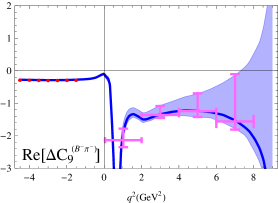
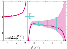
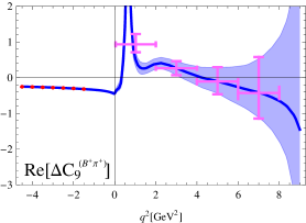
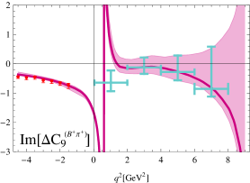
Figure 9: The real part (upper left, blue online) and imaginary part (upper right, red online) of $\Delta C^{B\pi}_{9}(q^{2})$ for $B^{-}\to\pi^{-}\ell^{+}\ell^{-}$. The solid line is the dispersion relation fitted to the results calculated at $q^{2}<0$ at the central input. The shaded area indicates the estimated 68% C.L. uncertainties obtained in the fit to the “data” points (dots,red online) at $q^{2}<0$. The values of $\Delta C^{B\pi}_{9}(q^{2})$ averaged over the $q^{2}$-bins are also shown. The lower panel contains the same plots for $B^{+}\to\pi^{+}\ell^{+}\ell^{-}$.

A few comments on the fit procedure of Eq. (41) are in order. Here we only discuss the $B^{\mp}\to\pi^{\mp}+\ell^{+}\ell^{-}$ decay, as the case of the neutral $B$ decays is very similar. We represent the results of our calculation at negative $q^{2}$ values as “data” points and perform a $\chi^{2}$ fit for our “model function” (dispersion relation), which is valid in both positive and negative $q^{2}$ regions, to the obtained points. As a technical remark: the fit is performed by collecting in the “data” all parts of Eq. (41) which contains no fit parameters, i.e. only the resonance contributions (amplitudes and phases) and the polynomial continuum parameters are included in the “model function”. Furthermore, we include the error correlation of the respective points at negative $q^{2}$, and, in addition, also of the parameter $f_{B\pi}^{+}(q^{2}=0)$. The errors and the correlation coefficients of the “data” are obtained by varying the input parameters within their intervals given in Table 1, while assuming no correlation between the parameters themselves. Thus, we include two correlated “data” sets in the fit for both charged $B$-meson transitions, namely, the real and imaginary parts of ${\cal H}^{(u)}$ and ${\cal H}^{(c)}$. We assume a gaussian error interval of the input parameters for this procedure and a maximum error correlation of 80$\%$ for the numerical stability, providing also a more conservative estimate. As expected, the error correlation between the “data” points is very large and usually exceeds 80$\%$. In addition, we find a positive correlation of, respectively, $\sim 1\%$($10\%$) for the real part and of $\sim 40\%$($1\%$) for the imaginary part of $H^{(u)}$ ($H^{(c)}$) with $f_{B\pi}^{+}(q^{2}=0)$. The global minima are acceptable with $\chi^{2}_{min}=1.93$ and $\chi^{2}_{min}=2.53$ for $u$ and $c$, respectively. The central values quoted here belong to the global minimum, whereas the 68 % C.L. error estimate includes all minima in the $\delta\chi^{2}<1$ region.

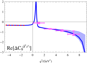
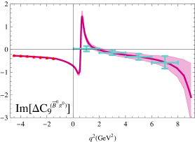
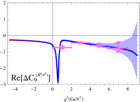
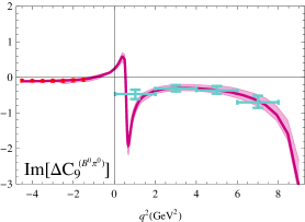
Figure 10: The same as in fig. 9 for $\bar{B^{o}}\to\pi^{0}\ell^{+}\ell^{-}$ (upper panel) and for $B^{o}\to\pi^{0}\ell^{+}\ell^{-}$ (lower panel).

7 Observables in $B\to\pi\ell^{+}\ell^{-}$

Having calculated the nonlocal amplitudes in a form of the function $\Delta C^{(B\pi)}_{9}(q^{2})$, we substitute this function in the amplitude (2) of the $B\to\pi\ell^{+}\ell^{-}$ decay and predict the observables in the accessible dilepton mass region (42).

The only element in the complete decay amplitude, that was not specified so far, is the ratio (8) of tensor and vector $B\to\pi$ form factors entering the contribution of the $O_{7\gamma}$ operator. To obtain it, we evaluate the ratio of LCSR’s for both form factors obtained in Ref. [28]. The $q^{2}$-dependence turns out to be negligible in the whole region of validity of the sum rules, which covers the region (42), and we obtain:

$$r_{T}(q^{2})\simeq r_{T}(0)=0.98\pm 0.02.$$ (43)

The observables in $B\to\pi\ell^{+}\ell^{-}$ include the differential branching fraction, direct $CP$-asymmetry and isospin asymmetry. Note that in SM the angular distribution in $B\to\pi\ell^{+}\ell^{-}$ at fixed $q^{2}$ is reduced to an overall factor $\left(1-\cos^{2}\Theta\right)$ in the double differential distribution where $\Theta$ is the angle between the momentum of the lepton $\ell^{-}$ and the momentum of the $B$-meson in the dilepton center mass frame. In particular, the forward-backward asymmetry in $B\to\pi\ell^{+}\ell^{-}$ vanishes in the SM. Hence, it is sufficient to calculate the dilepton invariant mass distribution of the branching fraction:

$$\frac{1}{\tau_{B^{-}}}\frac{dB(B^{-}\to\pi^{-}\ell^{+}\ell^{-})}{dq^{2}}=\frac{G_{F}^{2}\alpha_{\rm em}^{2}|\lambda_{t}|^{2}}{1536\pi^{5}m_{B}^{3}}|f^{+}_{B\pi}(q^{2})|^{2}\lambda^{3/2}(m_{B}^{2},m_{\pi}^{2},q^{2})$$

$$\times\Bigg{\{}\left|C_{9}+\Delta C_{9}^{B\pi}(q^{2})+\frac{2m_{b}}{m_{B}+m_{\pi}}C_{7}\,r^{T}_{B\pi}(q^{2})\right|^{2}+\left|C_{10}\right|^{2}\Bigg{\}}\,.$$ (44)

For $\bar{B}^{0}\to\pi^{0}\ell^{+}\ell^{-}$ the corresonding formula contains $\tau_{B^{0}}$ and an additional factor 1/2 reflecting the normalization of the $\bar{B}^{0}\to\pi^{0}$ form factor. The resulting plots are presented in Figs. 11, 12. Averaging the above distribution over $q_{1}^{2}\leq q^{2}\leq q_{2}^{2}$ yields the binned branching fraction defined, e.g., for $B^{-}\to\pi^{-}\ell^{+}\ell^{-}$ as:

$${\cal B}(B^{-}\to\pi^{-}\ell^{+}\ell^{-}[q_{1}^{2},q_{2}^{2}])\equiv\frac{1}{q_{2}^{2}-q_{1}^{2}}\int\limits_{q_{1}^{2}}^{q_{2}^{2}}dq^{2}\frac{dB(B^{-}\to\pi^{-}\ell^{+}\ell^{-})}{dq^{2}}\,.$$ (45)

The predicted binned branching fractions within the region (42) are presented in Table 4 for all four flavour/charge combinations.

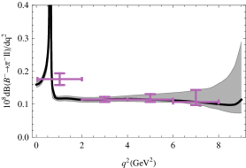
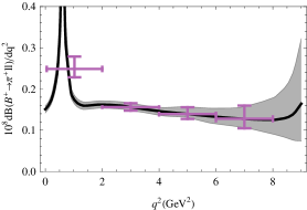
Figure 11: Dilepton invariant mass spectrum and binned branching fraction (in GeV${}^{\,-2}$) for $B^{-}\to\pi^{-}\ell^{+}\ell^{-}$ (left panel) and $B^{+}\to\pi^{+}\ell^{+}\ell^{-}$(right panel) with 68% C.L. errors (shaded region and error bars).

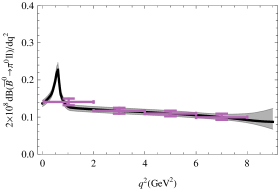
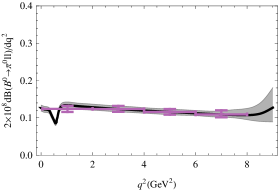
Figure 12: The same as in fig. 11 for $\bar{B}^{0}\to\pi^{0}\ell^{+}\ell^{-}$ (left panel) and $B^{0}\to\pi^{+}\ell^{+}\ell^{-}$ (right panel).

The most interesting characteristics of the $B\to\pi\ell^{+}\ell^{-}$ decay in SM is the $q^{2}$-dependent direct $CP$-asymmetry defined for the charged $B$-meson modes as:

$${\cal A}_{CP}^{(-+)}(q^{2})=\frac{\displaystyle d{B}(B^{-}\to\pi^{-}\ell^{+}\ell^{-})/dq^{2}-\displaystyle d{B}(B^{+}\to\pi^{+}\ell^{+}\ell^{-})/dq^{2}}{\displaystyle d{B}(B^{-}\to\pi^{-}\ell^{+}\ell^{-})/dq^{2}+\displaystyle d{B}(B^{+}\to\pi^{+}\ell^{+}\ell^{-})/dq^{2}}\,.$$ (46)

The asymmetry for the neutral $B$-meson modes denoted as ${\cal A}_{CP}^{(\bar{0}0)}(q^{2})$ has the same expression with $B^{-}\to\bar{B^{0}}$, $B^{+}\to B^{0}$. The results obtained for this observable are presented in Fig. 13.

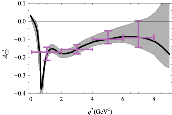
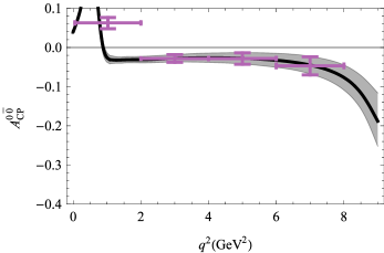
Figure 13: Direct $CP$-asymmetry in $B^{\pm}\to\pi^{\pm}\ell^{+}\ell^{-}$ (upper panel) and in $B^{\bar{0}0}\to\pi^{0}\ell^{+}\ell^{-}$ (lower panel).

Anticipating the future measurements of the $q^{2}$-averaged bins of $CP$-asymmetry, we also calculate

$${\cal A}_{CP}^{(-+)}[q_{1}^{2},q_{2}^{2}]=\frac{{\cal B}(B^{-}\to\pi^{-}\ell^{+}\ell^{-}[q_{1}^{2},q_{2}^{2}])-{\cal B}(B^{+}\to\pi^{+}\ell^{+}\ell^{-}[q_{1}^{2},q_{2}^{2}])}{{\cal B}(B^{-}\to\pi^{-}\ell^{+}\ell^{-}[q_{1}^{2},q_{2}^{2}])+{\cal B}(B^{+}\to\pi^{+}\ell^{+}\ell^{-}[q_{1}^{2},q_{2}^{2}])}\,,$$ (47)

and the analogous binned asymmetry ${\cal A}_{CP}^{\bar{0}0}[q_{1}^{2},q_{2}^{2}]$ for the neutral $B$-meson modes. Our predictions are collected in Table 4.

Bin [GeV2]	$[0.05,2.0]$	$[2.0,4.0]$	$[4.0,6.0]$	$[6.0,8.0]$	$[1.0,6.0]$
${\cal B}(B^{-})$	$0.176^{+0.018}_{-0.018}$	$0.114^{+0.008}_{-0.007}$	$0.114^{+0.016}_{-0.007}$	$0.107^{+0.036}_{-0.009}$	$0.126^{+0.013}_{-0.010}$
${\cal B}(B^{+})$	$0.249^{+0.030}_{-0.020}$	$0.156^{+0.009}_{-0.008}$	$0.139^{+0.016}_{-0.011}$	$0.128^{+0.030}_{-0.023}$	$0.168^{+0.016}_{-0.012}$
$2\times{\cal B}(\bar{B}^{0})$	$0.140^{+0.009}_{-0.009}$	$0.117^{+0.008}_{-0.008}$	$0.109^{+0.008}_{-0.008}$	$0.099^{+0.010}_{-0.007}$	$0.119^{+0.008}_{-0.008}$
$2\times{\cal B}(B^{0})$	$0.124^{+0.008}_{-0.008}$	$0.124^{+0.008}_{-0.008}$	$0.116^{+0.008}_{-0.007}$	$0.109^{+0.011}_{-0.008}$	$0.121^{+0.008}_{-0.008}$
${\cal A}_{CP}^{(-+)}$	$-0.171^{+0.027}_{-0.045}$	$-0.156^{+0.027}_{-0.024}$	$-0.099^{+0.047}_{-0.025}$	$-0.091^{+0.093}_{-0.053}$	$-0.143^{+0.035}_{-0.029}$
${\cal A}_{CP}^{(\bar{0}0)}$	$\phantom{-}0.063^{+0.014}_{-0.015}$	$-0.028^{+0.010}_{-0.010}$	$-0.028^{+0.015}_{-0.015}$	$-0.047^{+0.023}_{-0.023}$	$-0.008^{+0.013}_{-0.013}$
${\cal A}_{I}$	$-0.195^{+0.033}_{-0.035}$	$-0.020^{+0.031}_{-0.032}$	$-0.021^{+0.035}_{-0.053}$	$-0.021^{+0.060}_{-0.100}$	$-0.063^{+0.033}_{-0.040}$

Table 4: Binned branching fractions (in units of 10^-8 (GeV${}^{\,-2}$)), direct $CP$-asymmetry and isospin asymmetry of $B\to\pi\ell^{+}\ell^{-}$.

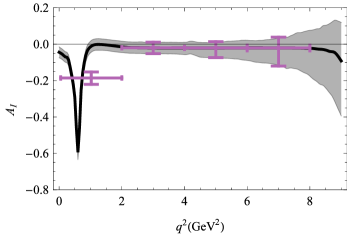
Figure 14: Differential isospin asymmetry for $B\to\pi\ell^{+}\ell^{-}$ decays.

Finally, an important indicator of the spectator-dependent nonlocal effects, such as weak annihilation, is a nonvanishing differential isospin asymmetry defined as:

$${\cal A}_{I}(q^{2})=\frac{2\displaystyle d\Gamma(\bar{B}^{0}\to\pi^{0}\ell^{+}\ell^{-})/dq^{2}-\displaystyle d\Gamma(B^{-}\to\pi^{-}\ell^{+}\ell^{-})/dq^{2}}{2\displaystyle d\Gamma(\bar{B}^{0}\to\pi^{0}\ell^{+}\ell^{-})/dq^{2}+\displaystyle d\Gamma(B^{-}\to\pi^{-}\ell^{+}\ell^{-})/dq^{2}}\,,$$ (48)

where the differential widths are understood as the CP-averaged ones. Our result is presented in Fig 14 and the corresponding $q^{2}$-bins of isospin asymmetry:

$${\cal A}_{I}[q_{1}^{2},q_{2}^{2}]=\frac{2\Gamma(\bar{B}^{0}\to\pi^{0}\ell^{+}\ell^{-}[q_{1}^{2},q_{2}^{2}])-\Gamma(B^{-}\to\pi^{-}\ell^{+}\ell^{-}[q_{1}^{2},q_{2}^{2}])}{2\Gamma(\bar{B}^{0}\to\pi^{0}\ell^{+}\ell^{-}[q_{1}^{2},q_{2}^{2}])+\Gamma(B^{-}\to\pi^{-}\ell^{+}\ell^{-}[q_{1}^{2},q_{2}^{2}])}\,$$ (49)

are given in Table 4.

Concluding the analysis of observables in $B\to\pi\ell^{+}\ell^{-}$, we notice that the magnitude of the predicted direct $CP$-asymmetry for the charged $B$ decay modes is quite visible; for the neutral $B$ decays this effect is expected to be small. In this and other observables our analysis generates large uncertainties in the region adjacent to $J/\psi$, whereas the uncertainties in the $\rho$ and $\omega$ region are significantly smaller. This is partly caused by the use of QCDF to fix the relative phase between the nonleptonic amplitudes with $\rho$ and $\omega$, which probably leads to a slight underestimate of the errors in the resonance region.

8 The $B\to\pi\nu\bar{\nu}$ decay

The semileptonic FCNC decay $B\to\pi\nu\bar{\nu}$ is closely related to the charged lepton channel. Theoretically, this process is a very clean test of the SM, involving a single effective operator similar to $O_{10}$, whereas the nonlocal effects studied above are absent. Hence, we are in a position to predict the branching fraction of this decay with a better accuracy than for the $B\to\pi\ell^{+}\ell^{-}$. The only hadronic input in $B\to\pi\nu\bar{\nu}$ is the vector $B\to\pi$ form factor. The LCSR form factor [19] given in (27), provides an extrapolation beyond the large recoil region up to the kinematical limit $q^{2}=(m_{B}-m_{\pi})^{2}$, revealing a good agreement with the lattice QCD results in the low recoil region. We use this form factor to predict the total branching fraction of the $B\to\pi\nu\bar{\nu}$ decay.

The effective Hamiltonian encompassing the $b\to d\nu\bar{\nu}$ transition in the SM can be written as:

$${\cal H}_{\rm eff}^{b\to d\nu\bar{\nu}}=-\frac{4G_{F}}{\sqrt{2}}\lambda_{t}C_{10\nu}\frac{\alpha_{\rm em}}{4\pi}(\bar{d}_{L}\gamma_{\mu}b_{L})(\bar{\nu}\gamma^{\mu}(1-\gamma_{5})\nu)\,,$$ (50)

with the (scale-independent) Wilson coefficient:

$$C_{10\nu}=-\frac{1}{\sin^{2}\Theta_{W}}\left(X_{0}(x_{t})+\frac{\alpha_{s}}{4\pi}X_{1}(x_{t})\right),$$ (51)

where $x_{t}=m_{t}^{2}/m_{W}^{2}$ and the functions $X_{0}(x)$ and $X_{1}(x)$ can be found in Ref. [12].

The differential branching fraction of the $B^{-}\to\pi^{-}\nu\bar{\nu}$ decay summed over neutrino flavours has the form:

$$\frac{1}{\tau_{B^{-}}}\frac{d{\cal B}(B^{-}\to\pi^{-}\nu\bar{\nu})}{dq^{2}} \equiv \frac{1}{\tau_{B^{-}}}\sum\limits_{\ell=e,\mu,\tau}\frac{d{\cal B}(B\to\pi\nu_{\ell}\bar{\nu}_{\ell})}{dq^{2}}$$

$$= \frac{G_{F}^{2}\alpha_{\rm em}^{2}}{256\pi^{5}m_{B}^{3}}|\lambda_{t}|^{2}|C_{10\nu}|^{2}|f^{+}_{B\pi}(q^{2})|^{2}\lambda^{3/2}(m_{B}^{2},m_{\pi}^{2},q^{2})\,.$$

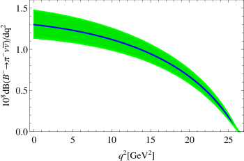
Figure 15: The differential branching fraction of the $B^{-}\to\pi^{-}\nu\bar{\nu}$ decay

Substituting the form factor $f^{+}_{B\pi}(q^{2})$ from Eq. (27), the numerical values of the Wilson coefficient $C_{10\nu}=-6.79$ and other parameters in Eq. (8), we obtain the differential branching fraction shown in Fig. 15. Integrating it over $0<q^{2}<(m_{B}-m_{\pi})^{2}$ we obtain:

$${\cal B}(B^{-}\to\pi^{-}\nu\bar{\nu})=2{\cal B}(B^{0}\to\pi^{0}\nu\bar{\nu})=(2.39^{+0.30}_{-0.28})\times 10^{-7}\,.$$ (53)

Despite the fact that this branching fraction is well within the reach of $B$-physics experiments, a severe problem is the identification of the final state with respect to the background.

9 Conclusion

In this paper we calculated the hadronic input for the rare FCNC decay $B\to\pi\ell^{+}\ell^{-}$ in the large recoil region of the pion, i.e., at small and intermediate lepton-pair masses up to the $J/\psi$ mass. We focused on the most difficult problem in the theory of these decays: the effects generated by a nonlocal overlap of the pointlike weak transition with the electromagnetic lepton-pair emission. At $q^{2}>0$ the nonlocality involves long distances, including the formation of hadronic resonances – the vector mesons. On the other hand, this part of the decay amplitude is not simply a background for the FCNC $b\to d\ell^{+}\ell^{-}$ transition, but provides the strong-interaction phase. The latter, combined with the CKM phase, generates the unique characteristics of the $B\to\pi\ell^{+}\ell^{-}$ decay in SM, that is the $q^{2}$-dependent direct CP-asymmetry, suppressed in the $b\to s\ell^{+}\ell^{-}$ decays.

To avoid the complications related to the long-distance part of the nonlocal effects, we employed the method used earlier in Ref. [9] for $B\to K\ell^{+}\ell^{-}$. The nonlocal contributions to $B\to\pi\ell^{+}\ell^{-}$ transitions were calculated one by one, combining QCDF and LCSRs at spacelike $q^{2}<0$, where the quark-level diagrams are well defined and the nonlocality is effectively reduced to the distances of $O(1/\sqrt{|q^{2}|})$. We also used the recently updated [19] $B\to\pi$ form factor from LCSR. The accuracy of our calculation is characterized by taking into account, in addition to the factorizable quark-loop effects and the factorizable NLO corrections, also the important nonfactorizable contributions: the soft gluon emission, spectator scattering and weak annihilation. We then combined the quark-level calculation with the hadronic dispersion relation and fitted the parameters of the latter to access the $q^{2}>0$ region. The main result of our calculation is presented in a form of the $q^{2}$-dependent and process-specific correction $\Delta C^{(B\pi)}_{9}(q^{2})$ to the Wilson coefficient of the semileptonic operator $O_{9}$. Apart from the numerical prediction for $\Delta C^{(B\pi)}_{9}(q^{2})$, we also estimated the uncertainties due to the input parameter variation. We predicted the observables in $B\to\pi\ell^{+}\ell^{-}$, including the differential branching fraction, direct $CP$-asymmetry and the isospin asymmetry. The main advantage of the method used in this paper is the possibility to access the $\rho,\omega$ resonance region and, simultaneously, to approach the charmonium region from below.

The accuracy of the calculation carried out in this paper can be improved further. On the theory side it is worth to calculate the nonlocal contributions using entirely LCSRs instead of the QCDF approximation. This will allow one to assess the missing power corrections. Such analysis is possible at least for the weak annihilation and for the hard spectator contributions. A more elaborated ansatz for the hadronic dispersion relation, including the radial excitations of light vector mesons, is also desirable. For that, more accurate data on the $B\to V\pi$ nonleptonic decays and a better understanding of the structure of various nonleptonic amplitudes are needed.

Let us compare our results with the two most recent analyses of the $B\to\pi\ell^{+}\ell^{-}$ decay. In [29], only the factorizable nonlocal contributions were taken into account, approximated by the quark-level diagrams at positive $q^{2}$, embedded in the short-distance coefficients. Only the differential branching fraction was calculated, with no prediction for the $CP$-asymmetry. In [6], the QCDF method was systematically used at positive $q^{2}$, therefore the resonance region of $q^{2}$ was not accessible. In the region between 2 GeV² and 6 GeV² the branching fraction obtained in [6] is somewhat smaller than our result, whereas the $CP$-asymmetry is close to our prediction.

We emphasize that our method produces a quantitative estimate of the nonlocal effects in the whole large-recoil region, starting from the kinematical threshold of the lepton-pair production. The price to pay is a model dependence of the ansatz for the dispersion relation, related to the nonleptonic $B\to V\pi$ decays. The function $\Delta C^{(B\pi)}_{9}(q^{2})$ obtained in this paper can be used in further analyses of the $B\to\pi\ell^{+}\ell^{-}$ decay, e.g., when adding to the decay amplitude in SM certain new physics contributions. But first of all, it will be very interesting to confront our prediction for the direct CP-asymmetry in $B\to\pi\ell^{+}\ell^{-}$ with the data. Note that the $b\to d\ell^{+}\ell^{-}$ effective interaction is also probed in $B_{d}\to\mu^{+}\mu^{-}$ decay. Its branching fraction measurement by LHCb and CMS collaborations [30] still leaves some room for new physics, making further studies of $b\to d\ell^{+}\ell^{-}$ decays very important.

Appendix A: Operators and CKM parameters

In Table 5 we list the operators entering the effective Hamiltonian (1), and their Wilson coefficients calculated at LO for three different renormalization scales, where $\alpha_{\rm em}=e^{2}/(4\pi)$ is the electromagnetic coupling, $g_{s}$ is the strong coupling. We use the standard conventions for the operators $O_{i}^{p}$ $(p=u,c)$ except the labeling of ${\cal O}_{1}^{p}$ and ${\cal O}_{2}^{p}$ is interchanged, as in [9]. In the quark-penguin operators $q=u,d,s,c,b$ and the mass of $d$-quark in ${\cal O}_{7\gamma}$ and ${\cal O}_{8g}$ is neglected. The sign conventions for covariant derivatives, $\gamma$-matrices, left- and right-handed components of the quark fields are the same as quoted in the Appendix of [9].

Operator	$\mu$ (GeV)	$2.5$	$3.0$	$4.5$
${\cal O}_{1}^{p}=\left(\bar{d}_{L}\gamma_{\mu}p_{L}\right)\left(\bar{p}_{L}\gamma^{\mu}b_{L}\right)$	$C_{1}$	1.169	1.148	1.111
${\cal O}_{2}^{p}=\left(\bar{d}_{L}^{i}\gamma_{\mu}p_{L}^{j}\right)\left(\bar{p}_{L}^{j}\gamma^{\mu}b_{L}^{i}\right)$	$C_{2}$	-0.360	-0.324	-0.255
${\cal O}_{3}=\left(\bar{d}_{L}\gamma_{\mu}b_{L}\right)\sum\limits_{q}\left(\bar{q}_{L}\gamma^{\mu}q_{L}\right)$	$C_{3}(\times 10^{-2})$	1.700	1.503	1.144
${\cal O}_{4}=\left(\bar{d}_{L}^{i}\gamma_{\mu}b_{L}^{j}\right)\sum\limits_{q}\left(\bar{q}_{L}^{j}\gamma^{\mu}q_{L}^{i}\right)$	$C_{4}(\times 10^{-2})$	-3.602	-3.271	-2.630
${\cal O}_{5}=\left(\bar{d}_{L}\gamma_{\mu}b_{L}\right)\sum\limits_{q}\left(\bar{q}_{R}\gamma^{\mu}q_{R}\right)$	$C_{5}(\times 10^{-2})$	0.985	0.910	0.756
${\cal O}_{6}=\left(\bar{d}_{L}^{i}\gamma_{\mu}b_{L}^{j}\right)\sum\limits_{q}\left(\bar{q}_{R}^{j}\gamma^{\mu}q_{R}^{i}\right)$	$C_{6}(\times 10^{-2})$	-4.829	-4.258	-3.236
${\cal O}_{7\gamma}=-\frac{e\,m_{b}}{16\pi^{2}}\left(\bar{d}_{L}\sigma^{\mu\nu}b_{R}\right)F_{\mu\nu}$	$C_{7}^{\rm eff}$	-0.356	-0.343	-0.316
${\cal O}_{8g}=-\frac{g_{s}m_{b}}{16\pi^{2}}\left(\bar{d}_{L}^{i}\sigma_{\mu\nu}(T^{a})^{ij}b^{j}_{R}\right)G^{a\,\mu\nu}$	$C_{8}^{\rm eff}$	-0.166	-0.160	-0.150
${\cal O}_{9}=\frac{\alpha_{\rm em}}{4\pi}\left(\bar{d}_{L}\gamma^{\mu}b_{L}\right)\left(\bar{\ell}\gamma_{\mu}\ell\right)$	$C_{9}$	4.514	4.462	4.293
${\cal O}_{10}=\frac{\alpha_{\rm em}}{4\pi}\left(\bar{d}_{L}\gamma^{\mu}b_{L}\right)\left(\bar{\ell}\gamma_{\mu}\gamma_{5}\ell\right)$	$C_{10}$	-4.493	-4.493	-4.493

Table 5: Effective operators and Wilson coefficients.

The electroweak parameters used to calculate the coefficients $C_{i}$ are [18]

$$\alpha_{\rm em}=\displaystyle\frac{1}{129}\,,\leavevmode\nobreak\ \leavevmode\nobreak\ \sin^{2}(\Theta_{W})=0.23126\,,\leavevmode\nobreak\ \leavevmode\nobreak\ m_{W}=80.385\mbox{ GeV}\,,$$

$$G_{F}=1.1663787\times 10^{-5}\mbox{ GeV}^{-2}\,,\leavevmode\nobreak\ m_{z}=91.186\mbox{ GeV}\,,\leavevmode\nobreak\ \leavevmode\nobreak\ m_{t}=173.3\mbox{ GeV}\,.$$ (54)

We use the CKM mixing matrix in term of Wolfenstein parameters

$$V_{\rm CKM}=\left(\begin{array}[]{ccc}1-\lambda^{2}/2&\lambda&A\lambda^{3}(\rho-i\eta)\\ -\lambda&1-\lambda^{2}/2&A\lambda^{2}\\ A\lambda^{3}(1-\rho-i\eta)&-A\lambda^{2}&1\\ \end{array}\right),$$

taking into account that $\rho\simeq\bar{\rho}\left(1+\lambda^{2}/2\right)$ and $\eta\simeq\bar{\eta}\left(1+\lambda^{2}/2\right)$ and using the current values [18] obtained from the global CKM fit:

$$\lambda=0.22537\pm 0.00061, A=0.814^{+0.023}_{-0.024},$$

$$\bar{\rho}=0.117\pm 0.021, \bar{\eta}=0.353\pm 0.013.$$ (55)

This results in the following combinations of CKM elements we use:

$$\lambda_{u}/\lambda_{t}=-0.0274-i\,0.3896,\quad|\lambda_{u}/\lambda_{t}|=0.3906,\quad{\rm arg}(\lambda_{u}/\lambda_{t})=-94.02^{\circ}$$

$$\lambda_{c}/\lambda_{t}=-0.9719+i\,0.3998,\quad|\lambda_{c}/\lambda_{t}|=1.0509,\quad{\rm arg}(\lambda_{c}/\lambda_{t})=157.64^{\circ}\,.$$ (56)

Appendix B: Amplitudes of $B\to\rho(\omega)\pi$ in QCDF

Here we present the expressions of the QCDF amplitudes [10] for the $B^{-}\to(\rho^{0},\omega)\pi^{-}$ nonleptonic decays. Our operators differs from the ones in [10] by a factor 1/4 whereas the labeling of $O_{1,2}$ is the same. The expressions for the parts of $B^{-}\to\rho^{0}\pi^{-}$ and $B^{-}\to\omega\pi^{-}$ amplitudes multiplying $\lambda^{p}$ ($p=u,c)$ are:

$$A_{B^{-}\rho\pi^{-}}^{p}=A_{\pi\rho}\bigg{(}\delta_{pu}\big{[}\alpha_{2}(\pi\rho)-\beta_{2}(\pi\rho)\big{]}-\alpha_{4}^{p}(\pi\rho)-\beta_{3}^{p}(\pi\rho)\bigg{)}$$

$$+A_{\rho\pi}\bigg{(}\delta_{pu}\big{[}\alpha_{1}(\rho\pi)+\beta_{2}(\rho\pi)\big{]}+\alpha_{4}^{p}(\rho\pi)+\beta_{3}^{p}(\rho\pi)\bigg{)},$$ (57)

$$A_{B^{-}\omega\pi^{-}}^{p}=A_{\pi\omega}\bigg{(}\delta_{pu}\big{[}\alpha_{2}(\pi\omega)+\beta_{2}(\pi\omega)\big{]}+2\alpha_{3}^{p}(\pi\omega)+\alpha_{4}^{p}(\pi\omega)+\beta_{3}^{p}(\pi\omega)\bigg{)}$$

$$+A_{\omega\pi}\bigg{(}\delta_{pu}\big{[}\alpha_{1}(\omega\pi)+\beta_{2}(\omega\pi)\big{]}+\alpha_{4}^{p}(\omega\pi)+\beta_{3}^{p}(\omega\pi)\bigg{)},$$ (58)

where the factorized combinations of form factors and decay constants are:

$$A_{\pi\rho(\omega)}=\frac{1}{2\sqrt{2}}f^{+}_{B\pi}(m_{\rho}^{2})f_{\rho(\omega)},\leavevmode\nobreak\ \leavevmode\nobreak\ \leavevmode\nobreak\ A_{\rho(\omega)\pi}=\frac{1}{2\sqrt{2}}A^{0}_{B\rho(\omega)}(0)f_{\pi}\,.$$ (59)

In addition to the already introduced notation, $A^{0}_{B\rho(\omega)}(0)$ in the above is the relevant $B\to\rho(\omega)$ form factor taken at $q^{2}=0$, neglecting the pion mass squared; for the $B\to\pi$ form factor we approximate $m_{\rho}^{2}=m^{2}_{\omega}$. The parameters $\alpha_{i}^{p}(M_{1}M_{2})$ are defined as follows [10]:

$$\alpha_{i}(M_{1}M_{2})=a_{i}(M_{1}M_{2}),\quad i=1,2,$$ (60)

$$\alpha_{3}^{p}=\left\{\begin{array}[]{ll}a_{3}^{p}(M_{1}M_{2})+a_{5}^{p}(M_{1}M_{2}),&\,{\rm if}\,M_{2}=\rho,\omega,\\ a_{3}^{p}(M_{1}M_{2})-a_{5}^{p}(M_{1}M_{2}),&\,{\rm if}\,M_{2}=\pi,\\ \end{array}\right.$$ (61)

$$\alpha_{4}^{p}=\left\{\begin{array}[]{ll}a_{4}^{p}(M_{1}M_{2})+r_{\chi}^{M_{2}}a_{6}^{p}(M_{1}M_{2}),&\,{\rm if}\,M_{2}=\rho,\omega,\\ a_{4}^{p}(M_{1}M_{2})-r_{\chi}^{M_{2}}a_{6}^{p}(M_{1}M_{2}),&\,{\rm if}\,M_{2}=\pi,\\ \end{array}\right.$$ (62)

where

$$r_{\chi}^{\pi}=\frac{2m_{\pi}^{2}}{m_{b}\,(m_{u}+m_{d})},\quad r_{\chi}^{\rho,\omega}=\frac{2m_{\rho,\omega}}{m_{b}}\frac{f_{\rho,\omega}^{\perp}}{f_{\rho,\omega}},$$ (63)

and $f_{\rho(\omega)}^{\perp}$ is the vector-meson transverse decay constant, defined as

$$\langle 0|\bar{q}\sigma^{\mu\nu}q|V(q)\rangle=ik^{\perp}(\varepsilon_{V}^{\mu}q^{\nu}-\varepsilon_{V}^{\nu}q^{\mu})f_{V}^{\perp}\,$$ (64)

with $k^{\perp}=1/\sqrt{2}$ for $q=u$, $V=\rho^{0},\omega$.

The quantities $a_{i}^{p}(M_{1}M_{2})$ have the form [2]:

$$a_{i}^{p}(M_{1}M_{2}) = \left(C_{i}+\frac{C_{i\pm 1}}{N_{c}}\right)N_{i}(M_{2})$$ (65)

$$+ \frac{C_{i\pm 1}}{N_{c}}\frac{C_{F}\alpha_{s}}{4\pi}\left[V_{i}(M_{2})+\frac{4\pi^{2}}{N_{c}}H_{i}(M_{1}M_{2})\right]+P_{i}^{p}(M_{2})\,,$$

where the upper (lower) signs apply when $i$ is odd (even); $N_{i}(M_{2})=0\,$ for $i=6$ and $M_{2}=\rho,\omega$ and $N_{i}(M_{2})=1$ in all other cases. The parameters $\beta_{i}^{p}(M_{1}M_{2})$ involve the weak annihilation contributions:

$$\beta_{i}^{p}(M_{1}M_{2})\equiv\frac{-f_{B}f_{M_{1}}f_{M_{2}}}{2\sqrt{2}m_{B}^{2}A_{M_{1}M_{2}}}b_{i}^{p}(M_{1}M_{2})\,.$$ (66)

The expressions used for the separate contributions in Eqs. (65), (66): $V_{i}(M_{2})$ (one-loop vertex correction), $H_{i}(M_{1}M_{2})$ (hard-spectator scattering), $P_{i}^{p}(M_{1}M_{2})$ (penguin contractions) and $b_{i}^{(p)}(M_{1}M_{2})$ (weak annihilation) can be found in [2, 10]. They were calculated in QCDF in terms of the perturbative kernels convoluted with the DAs of the $B$ meson, pion and $\rho$($\omega)$ meson. The latter DAs include the Gegenbauer moments $a_{2}^{\rho(\omega)}$ and $a_{2}^{\rho,\perp}$, similar to the ones that are contained in the pion twist-2 DA (25).

For the numerical analysis of the $B^{-}\to\rho(\omega)\pi$ amplitudes we need additional input parameters listed in Table 6, where, in order to decrease the uncertainty, the $A_{0}^{B\omega}(0)$ form factor is calculated multiplying the ratio $A_{0}^{B\omega}(0)/f_{+}^{(B\pi)}(0)$ obtained from the LCSRs with the $B$-meson DAs [23] with the form factor $f_{+}^{(B\pi)}(0)$ taken from the most accurate LCSR with pion DAs [19].

Parameter	Ref.
$(m_{u}+m_{d})(1\mbox{GeV})=7.0^{+1.4}_{-0.4}$ MeV	[18]
$f_{+}^{(B\pi)}(m_{\rho}^{2})=0.316\pm 0.021\hskip 56.9055pt$	[19]
$A_{0}^{B\rho}(0)=0.396^{+0.039}_{-0.031}$	[23]
$A_{0}^{B\omega}(0)\simeq A_{0}^{B\rho}(0)$
$f_{\rho}^{\perp}(1\mbox{GeV})=(0.160\pm 0.010)$ GeV	[31]
$f_{\omega}^{\perp}(1\mbox{GeV})=(0.145\pm 0.010)$ GeV
$a_{2}^{\rho,\omega}(1\mbox{GeV})=a_{2}^{\rho,\omega\perp}(1\mbox{GeV})=0.09^{+0.10}_{-0.07}$

Table 6: Additional input parameters related to the light vector mesons and used in the QCDF amplitudes of $B\to\rho(\omega)\pi$ decays.

References

- [1] R. Aaij et al. [LHCb Collaboration], JHEP 1212, 125 (2012).
- [2] M. Beneke, G. Buchalla, M. Neubert and C. T. Sachrajda, Phys. Rev. Lett. 83 (1999) 1914; Nucl. Phys. B 606 (2001) 245.
- [3] M. Beneke, T. Feldmann and D. Seidel, Nucl. Phys. B 612 (2001) 25.
- [4] M. Beneke, T. Feldmann and D. Seidel, Eur. Phys. J. C 41, 173 (2005).
- [5] C. Bobeth, G. Hiller and G. Piranishvili, JHEP 0712 (2007) 040; M. Bartsch, M. Beylich, G. Buchalla and D.-N. Gao, JHEP 0911, 011 (2009).
- [6] W. S. Hou, M. Kohda and F. Xu, Phys. Rev. D 90, no. 1, 013002 (2014)
- [7] J. Lyon and R. Zwicky Phys. Rev. D 88 (2013) 9, 094004.
- [8] A. Khodjamirian, T. Mannel, A. A. Pivovarov and Y.-M. Wang, JHEP 1009 (2010) 089.
- [9] A. Khodjamirian, T. Mannel and Y. M. Wang, JHEP 1302 (2013) 010.
- [10] M. Beneke and M. Neubert, Nucl. Phys. B 675 (2003) 333.
- [11] B. Grinstein, M.J. Savage and M.B. Wise, Nucl. Phys. B319 (1989) 271; M. Misiak, Nucl. Phys. B393 (1993) 23; A.J. Buras and M. Munz, Phys. Rev. D52 (1995) 186.
- [12] G. Buchalla, A. J. Buras and M. E. Lautenbacher, Rev. Mod. Phys. 68 (1996) 1125.
- [13] A. G. Grozin and M. Neubert, Phys. Rev. D 55, 272 (1997).
- [14] M. Beneke and T. Feldmann, Nucl. Phys. B 592 (2001) 3.
- [15] H. H. Asatryan, H. M. Asatrian, C. Greub and M. Walker, Phys. Rev. D 65 (2002) 074004.
- [16] H. M. Asatrian, K. Bieri, C. Greub and M. Walker, Phys. Rev. D 69 (2004) 074007.
- [17] D. Seidel, Phys. Rev. D 70 (2004) 094038.
- [18] K. A. Olive et al. [Particle Data Group Collaboration], Chin. Phys. C 38 (2014) 090001.
- [19] I. Sentitemsu Imsong, A. Khodjamirian, T. Mannel and D. van Dyk, JHEP 1502, 126 (2015).
- [20] P. Gelhausen, A. Khodjamirian, A. A. Pivovarov and D. Rosenthal, Phys. Rev. D 88, 014015 (2013) Errata in [Phys. Rev. D 89, 099901 (2014)], [Phys. Rev. D 91, no. 9, 099901 (2015)].
- [21] V. M. Braun, D. Y. Ivanov and G. P. Korchemsky, Phys. Rev. D 69, 034014 (2004).
- [22] A. Khodjamirian, T. Mannel, N. Offen and Y.-M. Wang, Phys. Rev. D 83, 094031 (2011).
- [23] A. Khodjamirian, T. Mannel and N. Offen, Phys. Rev. D 75, 054013 (2007).
- [24] H. Boos, T. Mannel and J. Reuter, Phys. Rev. D 70, 036006 (2004).
- [25] P. Frings, U. Nierste and M. Wiebusch, arXiv:1503.00859 [hep-ph].
- [26] C. Bruch, A. Khodjamirian and J. H. Kuhn, Eur. Phys. J. C 39, 41 (2005).
- [27] M. A. Shifman, A. I. Vainshtein and V. I. Zakharov, Nucl. Phys. B 147, 385, 448 (1979).
- [28] G. Duplancic, A. Khodjamirian, T. Mannel, B. Melic and N. Offen, JHEP 0804, 014 (2008).
- [29] A. Ali, A. Y. Parkhomenko and A. V. Rusov, Phys. Rev. D 89, no. 9, 094021 (2014).
- [30] V. Khachatryan et al. [CMS and LHCb Collaborations], Nature (2015) arXiv:1411.4413 [hep-ex].
- [31] P. Ball and R. Zwicky, Phys. Rev. D 71, 014029 (2005).