Light composite scalar boson from a see-saw mechanism in two-scale TC models.

Abstract

We consider the possibility of a light composite scalar boson arising from mass mixing between a relatively light and heavy scalar singlets in a see-saw mechanism expected to occur in two-scale Technicolor (TC) models. A light composite scalar boson can be generated when the TC theory features two technifermions species in different representations, $R_{1}$ and $R_{2}$, under a single technicolor gauge group, with characteristic scales $\Lambda_{1}$ and $\Lambda_{2}$. We determine the final composite scalar fields, $\Phi_{1}$ and $\Phi_{2}$, effective theory using the effective potential for composite operators approach. To generate a light composite scalar it is enough to have a walking (or quasi-conformal) behavior just for one of the technifermions representations.

The nature of the electroweak symmetry breaking is one of the most important problems in particle physics, and the $125$ GeV new resonance discovered at the LHC [1] has many of the characteristics expected for the Standard Model (SM) Higgs boson. If this particle is a composite or an elementary scalar boson is still an open question. Many models have considered the possibility of a light composite Higgs based on effective Higgs potentials as reviewed in Ref.[2]. The reason for the existence of the different models (or different potentials) for a composite Higgs, is a consequence of our poor knowledge of the strongly interacting theories, that is reflected in the many choices of parameters in the effective potentials. On the other hand the composite scalar boson mass can be calculated based on the dynamics of the theory [3], and this approach, although more complex, is more restrictive than the analysis of potential coefficients in several specific limits. Recently Higgs see-saw models have been proposed to explain possible deviations from the SM predictions[4]. In this paper we consider the possibility of a light TC scalar boson arising from mass mixing between a relatively light and heavy composite scalar singlets from a see-saw mechanism expected to occur in two-scale TC models[5, 6].

We will consider the formation of a light composite scalar boson when the TC theory features two technifermion species in different representations, $R_{1}$ and $R_{2}$, under a single technicolor gauge group, with characteristic scales $\Lambda_{1}$ and $\Lambda_{2}$. To determine the final effective theory for scalar composite fields [7], $\phi_{1}$ and $\phi_{2}$, we will review a few aspects of Ref.[8]. We start presenting the effective Lagrangian derived in the Ref.[8] in the case of only one variational effective composite field $\phi$

$$\Omega^{(\alpha)}_{R}=\int d^{4}x\left[\frac{1}{2}\right.\partial_{\mu}\Phi\partial^{\mu}\Phi-\frac{\lambda_{4VR}^{(\alpha)}}{4}\Phi^{4}-\left.\frac{\lambda_{6VR}^{(\alpha)}}{6}\Phi^{6}-...\right]\,.$$ (1)

where the final effective Lagrangian of Eq.(1) comes out when we normalize the scalar field $\phi$ according to [8]

$$\Phi\equiv[Z^{(\alpha)}]^{-\frac{1}{2}}\phi\,.$$ (2)

This normalization appears when we consider the effect of the kinetic term in the effective action [8].

The index $\alpha$ in Eq.(2) is related to most general asymptotic fermionic self-energy expression for a non-Abelian gauge theory [9, 10]:

$$\Sigma^{(\alpha)}(p^{2})\sim\mu\left(\frac{\mu^{2}}{p^{2}}\right)^{\alpha}\left[1+bg^{2}(\mu^{2})\ln\left(p^{2}/\mu^{2}\right)\right]^{-\gamma\cos(\alpha\pi)}\,\,\,,$$ (3)

describing all possible behaviors of any generic strongly interacting theory as discussed in the sequence. For $\alpha=1$ we obtain the form of the effective potential associated to the asymptotic self-energy behavior predicted by the operator product expansion (OPE) [11]

$$\Sigma^{(1)}(p^{2})\sim\frac{\mu^{3}}{p^{2}},$$ (4)

and for $\alpha=0$ we obtain the corresponding result to the following asymptotic expression

$$\Sigma^{(0)}(p^{2})\sim\mu\left[1+bg^{2}(\mu^{2})\ln\left(p^{2}/\mu^{2}\right)\right]^{-\gamma}\,.$$ (5)

The self-energy vary between these two extreme expressions as we change the number of fermions in the theory and when effective four fermion interactions start being important [12].

The asymptotic expression shown in Eq.(5) was determined in the appendix of Ref.[13] and it satisfies the Callan-Symanzik equation. It has been argued that Eq.(5) may be a realistic solution in a scenario where the chiral symmetry breaking is associated to confinement and the gluons have a dynamically generated mass [14, 15, 16]. This solution also appears when using an improved renormalization group approach in QCD, associated to a finite quark condensate [17], and it minimizes the vacuum energy as long as $n_{f}>5$ [18]. In Eqs.(3), (4) and (5) $\mu\approx\Lambda$, where $\Lambda$ is the characteristic mass scale of the strongly interacting theory forming the composite scalar boson, $\mu$ is the dynamical mass and is not an observable, moreover, from the QCD experience we may expect that they are of the same order. $g$ is the strongly interacting running coupling constant, $b$ is the coefficient of $g^{3}$ term in the renormalization group $\beta$ function, $\gamma=3c/16\pi^{2}b$, and $c$ is the quadratic Casimir operator given by $c=\frac{1}{2}\left[C_{2}(R_{1})+C_{2}(R_{2})-C_{2}(R_{3})\right]$ where $C_{2}(R_{i})$, are the Casimir operators for fermions in the representations $R_{1}$ or $R_{2}$ that form a composite boson in the representation $R_{3}$. We will consider only $SU(N)$ theories and the different $\alpha$ values in the interval of $0$ to $1$ will correspond to different self-energy behaviors, going from the extreme walking (or almost conformal $SU(N)$ theories [19]) to the standard OPE one [8].

The couplings ($\lambda_{nVR}^{(\alpha)}$) are given respectively by [8]

$$\lambda^{(0)}_{4VR} \equiv \lambda_{4V}^{(0)}[Z^{(0)}]^{2}=\frac{Nn_{f}}{4\pi^{2}}[Z^{(0)}]^{2}$$ (6)

$$\times\left[\left(\frac{1}{\beta(4\gamma-1)}+\frac{1}{2}\right)\right.$$

$$\left.-\frac{4\alpha}{\beta(4\gamma-1)}\left(\frac{1}{(4\gamma-2)}+2\gamma\right)\right],$$

$$\lambda^{(0)}_{6VR}\equiv\lambda_{6V}^{(0)}[Z^{(0)}]^{3}=-\frac{Nn_{f}}{4\pi^{2}}\frac{[Z^{(0)}]^{3}}{\Lambda^{2}{{}_{TC}}}\,\,\,,$$ (7)

and

$$\lambda^{(1)}_{4VR} \equiv \lambda_{4V}^{(1)}[Z^{(1)}]^{2}=\frac{Nn_{f}}{4\pi^{2}}[Z^{(1)}]^{2}$$ (8)

$$\times\left[\frac{1}{4}\left(1+\frac{c\alpha_{{}_{TC}}}{2\pi}\right)\right.$$

$$\left.-\frac{\beta}{4\alpha}\left(\gamma+\frac{c\alpha_{{}_{TC}}}{8\pi}(4\gamma+1)\right)\right]$$

$$\lambda^{(1)}_{6VR}\equiv\lambda_{6V}^{(1)}[Z^{(1)}]^{3}=-\frac{Nn_{f}}{4\pi^{2}}\frac{[Z^{(1)}]^{3}}{7\Lambda^{2}}\,\,\,,$$ (9)

in these expressions [8]

$$Z^{(0)}\approx\frac{4\pi^{2}\beta(2\gamma-1)}{N{n_{f}}}\,\,,\,\,Z^{(1)}\approx\frac{8\pi^{2}}{Nn_{f}}\left(1-\beta\gamma\right)$$ (10)

where we defined $\beta=bg^{2}$, $\alpha_{{}_{TC}}$ is the coupling constant of the technicolor interaction that forms the scalar composite.

Walking technicolor theories can have fermions belonging to different technicolor representations and, therefore, may have two different scales with characteristic chiral symmetry breaking scales $\Lambda_{1}(R_{1})<\Lambda_{2}(R_{2})$. In this proposal we are assuming that technifermions are in the representations $R_{1}$ and $R_{2}$ under a single technicolor gauge group as described in Ref.[5]. In the model proposed by Lane and Eichten, it is assumed that the TC running coupling constant is given by

$$\alpha_{TC}(p^{2})=\alpha_{2}\,\,{\rm when}\,\,p>\Lambda_{2}$$

$$\alpha_{TC}(p^{2})=\alpha_{1}\left[1+\beta^{1}_{0}\ln\left(\frac{p^{2}}{\Lambda^{2}_{1}}\right)\theta(p^{2}-\Lambda^{2}_{1})\right]^{-1}\!\!{\rm when}\,\Lambda_{1}<p<\Lambda_{2}$$

where $\alpha_{2}=\alpha(R_{2})=\frac{\pi}{3C_{2}(R_{2})}$, $\alpha_{1}=\alpha(R_{1})=\frac{\pi}{3C_{2}(R_{1})}$ and $\beta^{1}_{0}=\frac{\alpha_{1}}{6\pi}(11N_{TC}-4N_{1})$ and $N_{1}$ are technifermions doublets in the representation $R_{1}$. Note that the $N_{1}$ and $N_{2}$ doublets of technifermions belong to the complex TC representation $R_{1}$ and $R_{2}$, with dimensionality $d_{1}<d_{2}$. For a large enough number of $N_{1}$ doublets it is possible to obtain $\Lambda_{1}(R_{1})<<\Lambda_{2}(R_{2})$ [5] (or the decay constant $F_{1}<<F_{2}$) because

$$\frac{\Lambda_{2}}{\Lambda_{1}}\approx\exp{\left(\frac{6\pi}{(11N_{TC}-4N_{1})}\left[\alpha^{-1}(R_{2})-\alpha^{-1}(R_{1})\right]\right)},$$ (11)

in this case we can assume that the asymptotic technifermions self-energy behavior in representation $R_{1}$ can be described by Eq.(4), this hypothesis can be verified with the numerical results obtained in [5], where in the case (a) $R_{2}=A_{2}$ (second rank antisymmetric tensor representation), $N_{1}=6$, $N_{2}=2$ for $N_{TC}=5$, and we have $F_{2}/F_{1}\sim 7.7$. In Ref.[8] we have shown that the decay constants for the different asymptotic behavior of the self-energies (Eq.(4) $[\alpha=1]$, Eq.(5) $[\alpha=0]$) are given by

$$n_{d_{i}}F^{2}_{\alpha}=\left(1+\frac{\alpha}{2}\right)\frac{\Lambda^{2}_{TC}}{Z^{(\alpha)}}$$ (12)

where $n_{d_{i}}$ corresponds to the number of doublets of technifermions in the representation $i=1,2$. Therefore, for a two scale TC model this relationship implies

$$\frac{\sqrt{N_{2}}F_{2}}{\sqrt{N_{1}}F_{1}}\approx\sqrt{\frac{2Z^{(1)}}{3Z^{(0)}}}\frac{\Lambda_{2}}{\Lambda_{1}}.$$ (13)

Considering Eq.(10), together with the choice of parameters presented in the previous paragraph, the above expression leads to $F_{2}/F_{1}\sim 7.3$ in agreement with the numerical value described before. Therefore, for the analysis that we shall present in this work, the asymptotic expressions, (Eq.(4) $[\alpha=1]$, Eq.(5) $[\alpha=0]$), are a good approximation for determining the scalar spectrum of these type of two scale TC models.

At low energies we have an effective theory containing two different sets of composite scalars $\phi_{1}$ and $\phi_{2}$, and like the ones described in Ref.[5], we will assume an ETC gauge group containing $N_{1}$ technifermions doublets in the fundamental representation $R_{1}=F$, and $N_{2}$ technifermions doublets, assuming $N_{2}=1$ for $R_{2}$ representations (2-index antisymmetric $A_{2}$, 2-index symmetric $S_{2}$). The phenomenology of these type of models was already described in Ref.[5].

The fermionic content of the model that we will discuss contain two multiplets of technifermions in the representations $R_{1}$ and $R_{2}$ of the type

$$Q^{U}_{ETC}=\left(\begin{array}[]{c}{U^{a}_{R_{1}}}_{1}\\ \vdots\\ {U^{a}_{R_{1}}}_{i}\\ {U^{a}_{R_{2}}}_{1}\end{array}\right)_{L,R}\,\,,\,\,Q^{D}_{ETC}=\left(\begin{array}[]{c}{D^{a}_{R_{1}}}_{1}\\ \vdots\\ {D^{a}_{R_{1}}}_{i}\\ {D^{a}_{R_{2}}}_{1}\end{array}\right)_{L,R}$$ (22)

where $(a)$ is a technicolor index and $(i)$ is a flavour index. In this type of theory the ETC group would be $SU(N_{ETC})\supset SU(N_{TC}+N_{1}+N_{2})$, and in order to incorporate the mixing between $\phi_{1}$ and $\phi_{2}$, we must take into account the contributions of the ETC as displayed in Fig.(1). Remembering that the self-energy can also be related to the solutions of the Bethe-Salpeter equation, we can observe that the scalar boson $\phi_{1}$, formed by the fermions in the representation $R_{1}$ receive contributions of the condensates of the two different representations, as shown in Fig.(1).

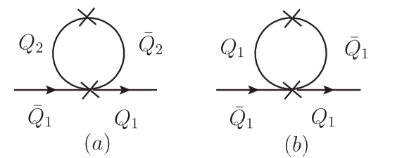
Figure 1: ETC (effective four-fermion) contributions to the mixing of scalars in the representations $R_{1}$ and $R_{2}$

We can detail a little bit more the comment of the previous paragraph and the behavior of the diagrams in Fig.(1). The $Q_{1}$ techniquarks will receive a dynamical mass due to the usual TC contribution and to the two diagrams in Fig.(1), that we indicate by

$$\Sigma_{Q_{1}}(p)\approx\Sigma^{TC}_{Q_{1}}(p)+\zeta\Sigma_{Q_{2}}+\xi\Sigma_{Q_{1}},$$ (23)

where $\zeta$ and $\xi$ are calculable constants. In the above expression the first one is the usual TC contribution due to condensation of $Q_{1}$ techniquarks in the representation $R_{1}$. The second comes from the ETC interaction with $Q_{2}$ techniquarks condensating in the representation $R_{2}$ and the third one is the $Q_{1}$ contribution from ETC interactions. Suppose now that the $Q_{1}$ techniquarks self-energy does not have a walking behavior, i.e. $\Sigma_{Q_{1}}(p^{2})$ is given by Eq.(4), therefore the $Q_{1}$ ETC contribution to $\Sigma_{Q_{1}}(p)$, Fig.(1b) will be giving by [10]

$$\xi\Sigma_{Q_{1}}\propto O(\frac{\Lambda^{3}_{1}}{\Lambda^{2}_{ETC}})<<1\,,$$ (24)

which is totally negligible.

We can now consider the effect of $Q_{2}$ technifermions in the representation $R_{2}$. This contribution is represented by the diagram of Fig.(1a), where we may have an extreme walking behavior for the $Q_{2}$ technifermions. In this case the correction due to ETC will be dominated by a self-energy of the type given by Eq.(5) resulting in [10]

$$\zeta\Sigma_{Q_{2}}\approx\Lambda_{2}\left(\frac{C_{ETC}}{C_{2R_{2}}}\left(\frac{\alpha_{ETC}(\Lambda^{2}_{ETC})}{\alpha_{TC}(\Lambda^{2}_{ETC})}\right)^{\gamma_{2}}\right).$$ (25)

Therefore the ETC correction ($\zeta\Sigma_{Q_{2}}$) plays a role similar of a bare mass term for the $\Sigma_{Q_{1}}(p)$ self-energy, i.e. a very hard self-energy! A similar reasoning may also be applied to the $\Sigma_{Q_{2}}(p)\approx\Sigma^{TC}_{Q_{2}}(p)+\kappa\Sigma_{Q_{1}}$. Although only one of the technifermions representations of one given TC group has a walking behavior and this group belongs to an ETC theory, at the end both technifermions representations will have asymptotically hard self-energies. In the following we will consider that the technifermions associated to the representation $R_{1}$ are in the fundamental representation with a self-energy behaving as the one of Eq.(4), and $\Sigma_{Q_{2}}(p)\approx\Sigma^{TC}_{Q_{2}}(p)$ behaving as Eq.(5) .

The different terms that are going to appear in the effective action are momentum integrals of different powers of the self-energies $\Sigma(p)$ [7], which are going to be represented as $[\phi_{i}\Sigma_{i}(p)]^{n}$, where $\phi_{i}$ acts like a dynamical effective scalar field (expanded around its zero momentum value) [8, 13], and it is interesting to verify how it is going to be the behavior of the $\Sigma_{i}^{4}(p)$ term (as a function of the momentum), which is the leading term of the effective potential [8, 13]. The fourth power of the self-energy associated to the fields $\phi_{1}$ and $\phi_{2}$, where the index $1$ will be related to technifermions with (in principle) a soft self-energy ($\alpha=1$), and the index $2$ will be related to technifermions in a representation $R_{2}=S_{2}$ or $R_{2}=A_{2}$, with a hard self-energy ($\alpha=0$), will be written as

$$\Sigma^{4}_{1}(p^{2})= \left(\Lambda_{1}f(p)+a_{ETC}\Lambda_{2}\right)^{4}\approx\Lambda^{4}_{1}f^{4}(p)+$$

$$4a_{ETC}\Lambda^{3}_{1}\Lambda_{2}f^{3}(p)+6a^{2}_{ETC}\Lambda^{2}_{1}\Lambda^{2}_{2}f^{2}(p)+...$$

$$\Sigma^{4}_{2}(p^{2})= \Lambda^{4}_{2}\left[1+\beta_{0}(R_{2})\ln\left(\frac{p^{2}}{\Lambda_{2}}\right)\right]^{-4\gamma_{2}}$$

where we defined $f(p)=\Lambda^{2}_{1}/p^{2}$ and $a_{ETC}$ is the ratio of Casimir operators and couplings of Eq.(25).

After some lengthy calculation, that follows the same steps delineated in Ref.[8], we obtain the following effective Lagrangian using the self-energies described previously

$$\Omega(\Phi_{1},\Phi_{2})= \int d^{4}x\left[\frac{1}{2}\partial_{\mu}\Phi_{1}\partial^{\mu}\Phi_{1}+\frac{1}{2}\partial_{\mu}\Phi_{2}\partial^{\mu}\Phi_{2}\right.$$ (26)

$$\left.-\frac{\lambda^{R_{1}}_{4n}}{4}Tr\Phi_{1}^{4}-\frac{\lambda^{R_{2}}_{4n}}{4}Tr\Phi_{2}^{4}-\frac{\lambda^{R_{1},R_{2}}_{4n}}{4}Tr\Phi_{1}^{2}\Phi_{2}^{2}\right.$$

$$\left.-\frac{\lambda^{R_{1}}_{6n}}{4}Tr\Phi_{1}^{6}-\frac{\lambda^{R_{2}}_{6n}}{4}Tr\Phi_{2}^{6}\right].$$

In Eq.(26) we included the contribution of the kinetic terms in the effective action [13]. The inclusion of these terms lead to the normalization condition

$$\Phi_{i}=\frac{\phi_{i}}{Z^{1/2}(R_{i})},$$ (27)

and the coefficients $\lambda^{R_{i}}_{4,6}$ and $\lambda^{R_{1},R_{2}}_{4}$ are the following

$$\lambda^{R_{1}}_{4}=\frac{N_{TC}N_{1}}{2\pi^{2}}\frac{1}{4}$$

$$\lambda^{R_{2}}_{4}=\frac{N_{TC}N_{2}}{2\pi^{2}}\left(\frac{1}{\beta(4\gamma_{2}-1)}+\frac{1}{2}\right)$$

$$\lambda^{R_{1},R_{2}}_{4}=\frac{3N_{TC}N_{1}}{4\pi^{2}}\left(\frac{C_{ETC}}{C_{2R_{2}}}\left(\frac{\alpha_{ETC}(\Lambda^{2}_{ETC})}{\alpha_{TC}(\Lambda^{2}_{ETC})}\right)^{\gamma_{2}}\right)^{2}$$

$$\lambda^{R_{1}}_{6}=-\frac{N_{TC}N_{1}}{2\pi^{2}}\frac{1}{7\Lambda^{2}_{1}}$$

$$\lambda^{R_{2}}_{6}=-\frac{N_{TC}N_{2}}{2\pi^{2}}\frac{1}{\Lambda^{2}_{2}}$$

where for the representations $i=1,2$ we have

$$b_{i}=\frac{1}{48\pi^{2}}\left(11N_{TC}-8T(R_{i})N_{i}\right)$$

$$\gamma_{i}=\frac{3C(R_{i})}{16\pi^{2}b_{i}}$$

$$b_{ETC}=\frac{1}{48\pi^{2}}\left(11N_{ETC}-8T(R_{1})N_{1}-8T(R_{2})N_{2}\right)$$

$$\alpha_{ETC}(\Lambda_{ETC})=\frac{\alpha_{ETC}(\Lambda_{2})}{\left[1+4\pi b_{ETC}\alpha_{ETC}(\Lambda_{2})\ln\left(\frac{\Lambda^{2}_{ETC}}{\Lambda^{2}}\right)\right]}$$

$$\alpha_{TC}(\Lambda_{ETC})\approx\alpha_{TC}(\Lambda_{2})\approx\frac{\pi}{3C_{2}(R_{2})},$$ (29)

in the previous expressions we assume the MAC hypothesis and the normalized constants $\lambda^{R_{i}}_{4n,6n}$ and $\lambda^{R_{1},R_{2}}_{4n}$ are identified as

$$\lambda^{R_{i}}_{4n}=\lambda^{R_{i}}_{4}Z^{2}(R_{i})$$

$$\lambda^{R_{1},R_{2}}_{4n}=\lambda^{R_{1},R_{2}}_{4}Z(R_{1})Z(R_{2})$$

$$\lambda^{R_{i}}_{6n}=\lambda^{R_{i}}_{6}Z^{3}(R_{i})$$

and the normalization coefficients $Z(R_{i})$ are

$$Z(R_{1})=\frac{16\pi^{2}}{N_{TC}N_{1}}\left(1-\beta_{1}\gamma_{1}\right)$$

$$Z(R_{2})=\frac{8\pi^{2}\beta_{2}(2\gamma_{2}-1)}{N_{TC}N_{2}}.$$ (31)

The most important characteristic of this effective Lagrangian is the mixing term

$$\lambda^{R_{1},R_{2}}_{4}=\frac{3N_{TC}N_{1}}{2\pi^{2}}\left(\frac{C_{ETC}}{C_{2R_{2}}}\left(\frac{\alpha_{ETC}(\Lambda^{2}_{ETC})}{\alpha_{TC}(\Lambda^{2}_{ETC})}\right)^{\gamma_{2}}\right)^{2}.$$ (32)

This mixing is the one that defines the splitting between the effective fields $\phi_{1}$ and $\phi_{2}$, as discussed by Foadi and Frandsen [6], whereas within the approach taken in this work their parameter $\delta$ [6], characterizing the mixing in the mass matrix, is

$$\delta=\frac{\lambda^{R_{1},R_{2}}_{4n}}{\sqrt{\lambda^{R_{1}}_{4n}\lambda^{R_{2}}_{4n}}}.$$ (33)

We emphasize that this mixing appears naturally in a two-scale TC model, where it is enough that one of the scales, and the fermionic representation associated to it, has an extreme walking behavior and the TC group is embedded into an ETC theory. In this work we will be considering two different situations for technifermions in $R_{2}$ representation, case (a) [with $R_{2}=A_{2}$, $N_{2}=1$ , $N_{1}=10$] and case (b) [with $R_{2}=S_{2}$, $N_{2}=1$ , $N_{1}=8$]. This choice of fermionic content guarantees the preservation of asymptotic freedom and walking behavior.

In the case of a large mixing we certainly can obtain a light scalar composite boson with a few hundred GeV mass. We show, as an example, in Fig.(2) the behaviour of the parameter $\delta$ in the case (a).

Figure 2: In this figure we show the behavior of the mixing term $\delta$ as a function of $N_{TC}$(x-axis) and $\Lambda_{ETC}$ (y-axis). The figure corresponds to the case (a), where $R_{2}=A_{2}$, $N_{2}=1$ , $N_{1}=10$. From this figure it is possible to verify that for the region compatible with the experimental limit on to Higgs mass (see Fig.(3)), $\delta\approx 0.4$ and $\Lambda_{ETC}>500TeV$.

Considering Eq.(11), and $F_{2}\sim 250GeV$, we note that the scale $\Lambda_{2}$ is defined by

$$N_{2}F^{2}_{2}=\frac{\Lambda^{2}_{2}}{Z^{(0)}}$$ (34)

which leads to

$$\Lambda_{2}=\frac{2\pi F_{2}\sqrt{\beta(2\gamma-1)}}{\sqrt{N_{TC}}}\sim\frac{O(TeV)}{\sqrt{N_{TC}}}.$$ (35)

Finally, assuming

$$M^{2}_{\Phi_{i}}=\frac{\partial^{2}\Omega(\Phi_{i})}{\partial\Phi^{2}_{i}}\left|{}_{\Phi=\Phi_{min}}\right.$$ (36)

we obtain

$$M^{2}_{{}_{\Phi_{i}}}\approx 2\lambda^{R_{i}}_{4n}\left(\frac{\lambda^{R_{i}}_{4n}}{\lambda^{R_{i}}_{6n}}\right).$$ (37)

We can write the following mass matrix in the base formed by the composite scalars ($\Phi_{1}$) and ($\Phi_{2}$)

$$M^{2}_{\Phi_{1},\Phi_{2}}=\left(\begin{array}[]{cc}M^{2}_{1}&M^{2}_{12}\delta\\ \delta M^{2}_{12}&M^{2}_{2}\end{array}\right).$$ (40)

The eigenvalues of this matrix provide the mass spectrum for the light scalar $(H_{1})$ and heavy $(H_{2})$, including the mixing effect parametrized by $\delta$, where

$$M^{2}_{i}=2\lambda^{R_{i}}_{4n}\left(\frac{\lambda^{R_{i}}_{4n}}{\lambda^{R_{i}}_{6n}}\right)$$

$$M^{2}_{12}=M_{1}M_{2}.$$

From the above equations we can determine the mass spectrum for the scalar bosons, $H_{1}(R_{1})$ and $H_{2}(R_{2})$, which are the diagonalized masses of the scalars $\Phi_{1}$ and $\Phi_{2}$ and these results are shown in Figs. (3) and (4), where we present the mass spectrum obtained for the light and heavier composite scalars $H_{1}(R_{1})$ and $H_{2}(R_{2})$ in the cases where $R_{1}=F$, $R_{2}=A_{2}$ or $R_{2}=S_{2}$.

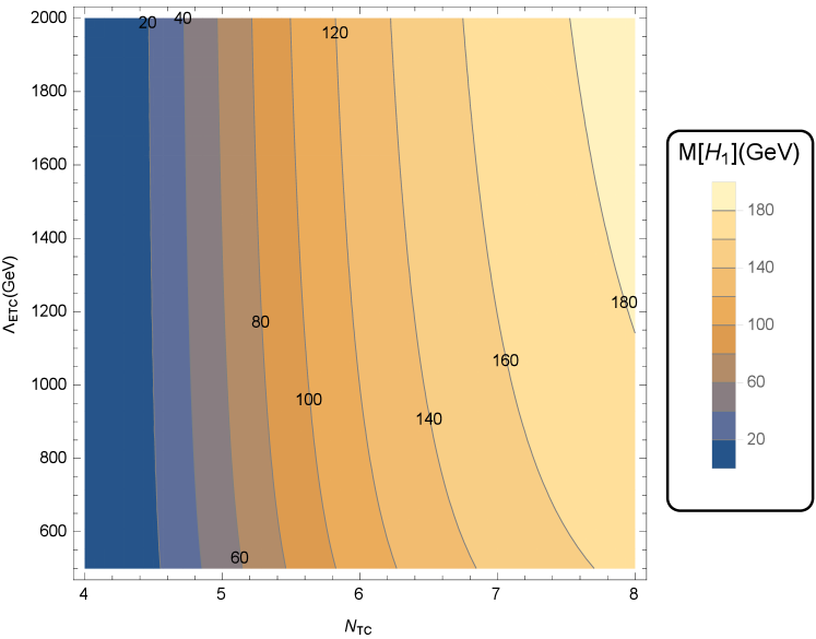
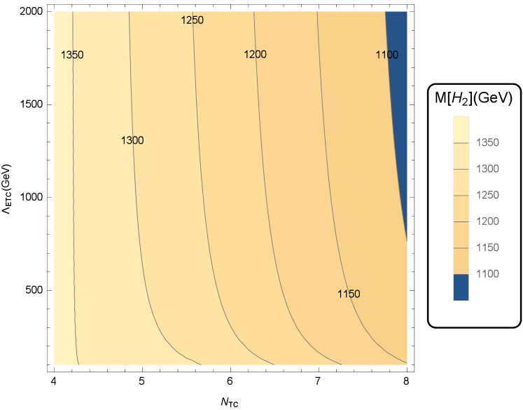
Figure 3: The light composite scalar $H_{1}$ and heavier composite scalar $H_{2}$ regions of masses as a function of the parameters $N_{TC}$ and $\Lambda_{ETC}$ in the case (a), which is similar to the one considered by Lane and Eichten in Ref.[5].

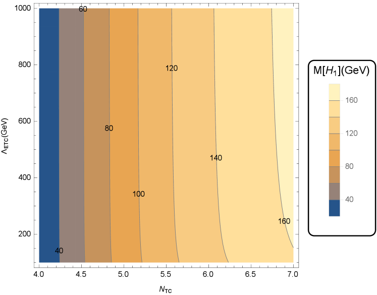
Figure 4: Light ($H_{1}$) and heavy ($H_{2}$) scalar composite region of masses in the case (b) [$R_{2}=S_{2}$, $N_{2}=1$ , $N_{1}=8$] as a function of the parameters $N_{TC}$ and $\Lambda_{ETC}$.

In this work we have computed an effective action for a composite scalar boson system formed by two technifermion species in different representations, $R_{1}$ and $R_{2}$, under a single technicolor gauge group with characteristic scales $\Lambda_{1}$ and $\Lambda_{2}$ as the original proposal presented in Ref.[5]. The calculation is based on an effective action for composite operators[8], the novelty of the calculus presented in this work is that we included technifermions in different representations, $R_{1}$ and $R_{2}$, under a single technicolor gauge group. Our main results are described in Figs. (3) , (4). The mixing between the composite scalar bosons $\Phi_{1}$ and $\Phi_{2}$ is responsible for generating a light scalar composite of a few hundred GeV mass. A particular example of the values of this mixing is shown in Fig.(2). To obtain a large mixing it is enough that one of the technifermions representations has a walking behavior and the TC group is embedded in an ETC theory. At the end the technifermions of both representations will have asymptotically hard self-energies.

For a set of parameters similar to the ones used in Ref.[5] in the case $R_{2}=A_{2}$, we obtain the same TC group necessary to generate the walking behavior, $SU(6)_{TC}$, leading to $M_{H_{1}}\sim{\cal{O}}(100)$ GeV . This result reinforces the validity of hypothesis discussed below Eq.(13), and this is a consequence of the walking (or quasi-conformal) technicolor theory. Furthermore, the large anomalous dimensions $\gamma_{m}$ enhance light-scale technipion masses, $M_{\pi 1}>M_{\rho 1}-M_{W}$, where technirho mass $M_{\rho 1}\sim 250GeV$. The difference between the results obtained for the representations $R_{2}=A_{2}$ and $R_{2}=S_{2}$ is that in the $A_{2}$ case we obtain a light scalar mass only with a large ETC scale $(\Lambda_{ETC}>10^{3}TeV)$. For the heavy scalar bosons obtained with $R_{2}=S_{2}$ or $R_{2}=A_{2}$ we expect the mass to be in the range $[1200-1300]$ GeV.

It is interesting to shortly digress the case where this light scalar composite could be related to the $125$ GeV scalar resonance found at CERN. The observed boson has couplings to the top and bottom quarks of the order expected for a fundamental SM Higgs boson. The fermionic couplings in a realistic composite scalar model will involve the ETC group and a delicate alignment of the $H_{1}$ and $H_{2}$ vacua, where only $H_{2}$ may resemble a fundamental scalar. Our model is far away from a realistic model since we have not defined a specific ETC theory. However we can imagine a theory where the fermionic masses are not generated as usual, by different ETC mass scales, but a horizontal symmetry is introduced, as in [20], where the top quark (or the third fermionic generation) obtain its mass associated to a large ETC scale, or coupling mostly to the $H_{2}$ scalar composite, without generating undesirable four-fermion interactions incompatible with the experimental data. We have also to remember that when QCD is embedded into a large ETC group together with the different TC fermionic representations, we actually will be dealing with tree different set of scales, all of them with possible hard asymptotic contributions to the self-energies due to the mechanism discussed here, where the horizontal symmetry will act in order to provide the desirable fermionic couplings with the different scales. Of course, a detailed model in this direction is not easy to obtain and is out of the scope of this work.

In Ref.[16] we considered the possibility of generating a light TC scalar boson based on the use of the Bethe-Salpeter equation and its normalization condition, as a function of the $SU(N)$ group and the respective fermionic representation. In that work we discussed how difficult was to generate a light scalar composite; what was possible, for example in the case of fermions in the fundamental representation, only for a specific (and large) number of fermions and moderate $N_{TC}$. In this work we discuss a different possibility for generating a light composite in a type of see saw mechanism in a two-scale TC model, and a small scalar mass is again generated in similar conditions. It is possible that the mixing mechanism that we propose here may be extended to models with more than one TC group, although it is also possible to envisage that in this case we shall need a more complex ETC interaction in order to mix the different groups.

A point to be noted is that the possibility of obtaining a light composite scalar according to the approach discussed in Ref.[16], first obtained in [21], is that this result is a direct consequence of extreme walking (or quasi-conformal) technicolor theories, where the asymptotic self-energy behavior is described by Eq.(5), this same behavior must also be present to generate a large mixing ($\delta$), necessary to obtain a light scalar boson mass of approximately a few hundred GeV in a two-scale model. In this work we identified that, regardless of the approach used for generating a light composite scalar boson, the behavior exhibited by extreme walking (or quasi-conformal) technicolor theories is the main feature needed in any model to produce a light composite scalar boson.

References

[1] ATLAS Collaboration, Phys. Lett. B 716, 1 (2012); CMS Collaboration, arXiv:1207.7235
[hep-ex].
[2] B. Bellazzini, C. Csáki and J. Serra, Eur. Phys. J. C 74, 2766 (2014).
[3] A. Doff and A. A. Natale, Phys. Lett. B 677, 301 (2009).
[4] P. S. Bhupal Dev, Dilip Kumar Ghosh, Nobuchika Okadac and Ipsita Sahab, JHEP 0150, 03 (2013);
Rabindra N. Mohapatra and Yongchao Zhanga, JHEP 0072, 06 (2014).
[5] K. Lane and E. Eichten, Phys. Lett. B 222, 274 (1989).
[6] Roshan Foadi and Mads T. Frandsen, arXiv:1212.0015v1.
[7] J. M. Cornwall, R. Jackiw and E. T. Tomboulis, Phys. Rev. D 10, 2428 (1974).
[8] A. Doff, A. A. Natale and P. S. Rodrigues da Silva, Phys. Rev. D 77, 075012(2008).
[9] A. Doff and A. A. Natale, Phys. Lett. B 537, 275 (2002).
[10] A. Doff and A.A. Natale, Phys.Rev. D68 077702, (2003).
[11] H. D. Politzer, Nucl. Phys. B 117, 397 (1976).
[12] T. Takeuchi, Phys. Rev. D 40, 2697 (1989); K.-I.Kondo, S. Shuto and K. Yamawaki, Mod. Phys.
Lett. A 6, 3385 (1991).
[13] J. M. Cornwall and R. C. Shellard, Phys. Rev. D 18, 1216 (1978).
[14] A. Doff, F. A. Machado and A. A. Natale, Annals of Physics
327 1030 (2012).
[15] A. Doff, F. A. Machado and A. A. Natale, New. J. Phys.
14, 103043 (2012).
[16] A. Doff, E. G. S. Luna and A. A. Natale, Phys. Rev. D 88, 055008 (2013).
[17] L.-N. Chang and N.-P. Chang, Phys. Rev. D 29, 312
(1984); Phys. Rev. Lett. 54, 2407 (1985); N.-P. Chang and D. S. Li,
Phys. Rev. D 30, 790 (1984).
[18] J. C. Montero, A. A. Natale, V. Pleitez and S. F. Novaes, Phys. Lett. B 161, 151 (1985).
[19] D. D. Dietrich and F. Sannino, Phys.Rev.D 75, 085018 (2007).
[20] A. Doff and A. A. Natale, Eur. Phys. J. C 32, 417 (2003).
[21] A. Doff, A. A. Natale and P. S. Rodrigues da Silva, Phys. Rev. D 80, 055005 (2009).