Center clusters in full QCD at finite temperature and background magnetic field

Abstract

We study the center structure of full dynamical QCD at finite temperatures and nonzero values of the background magnetic field using continuum extrapolated lattice data. We concentrate on two particular observables characterizing center clusters: their fractality and the probability for percolation. For temperatures below and around the transition region, the fractal dimension is found to be significantly smaller than three, leading to a vanishing mean free path inside the cluster structure. This finding might be relevant for center symmetry-based models of heavy-ion collisions. In addition, the percolation probability is employed to define the transition temperature and to map out the QCD phase diagram in the magnetic field-temperature plane.

I Introduction

Quantum chromodynamics (QCD) is the theory describing strongly interacting matter. QCD predicts the existence of a finite temperature transition that separates the low-energy confined regime and the deconfined quark-gluon-plasma (QGP) phase. The properties of this transition are relevant for the evolution of the early universe and are also probed by contemporary heavy-ion collision experiments, both at RHIC and at the LHC.

Following the conjecture that the deconfinement transition in the gluonic sector is related to the magnetic transition of a corresponding spin system Svetitsky and Yaffe (1982); Yaffe and Svetitsky (1982), and the finding that the latter can be understood in terms of cluster percolation Fortuin and Kasteleyn (1972), it was proposed that the gluonic field configurations of QCD can be characterized by center clusters and that the deconfinement transition may be understood as a percolation phenomenon Bhattacharya et al. (1991). In this description confinement manifests itself in small and uncorrelated clusters, while the deconfined regime exhibits a large cluster that percolates and induces long-range correlations. The center structure of the QGP was also incorporated in models of heavy-ion collisions Gupta et al. (2010); Asakawa et al. (2013) and was argued to explain various properties of the plasma phase including its low shear viscosity and high (color) opacity Asakawa et al. (2013). The main ingredient in this kind of models is the scattering of partons on the cluster walls, characterized by a mean free path.

Besides the temperature, another parameter relevant for heavy-ion phenomenology is the background (electro)magnetic field generated by spectator particles in off-central collisions. Strong magnetic fields are also thought to have existed in the early stages of the universe and thus their effects on the QGP are of interest for cosmology as well. For recent reviews on the role of magnetic fields for strongly interacting matter see, e.g., Refs. Kharzeev et al. (2013); Andersen et al. (2014).

In this paper we perform numerical lattice simulations to study center clusters in $2+1$-flavor QCD and determine their response to nonzero temperatures and background magnetic fields. We confirm that the clusters are not three-dimensional objects but instead have a fractal nature, as has already been observed in pure gauge theory (see, e.g., Ref. Endrődi et al. (2014)). We demonstrate that as a consequence of this fractality the mean free path inside the clusters vanishes for temperatures and magnetic fields relevant for heavy-ion phenomenology. Furthermore, we propose a new observable for determining the transition temperature in full QCD and use it to map out the phase diagram in the magnetic field-temperature plane.

II Center clusters

The concept of center clusters relies on the center symmetry of pure gauge theory, formulated in Euclidean space-time at a nonzero temperature $T$. Center symmetry denotes the invariance of the action under topologically non-trivial transformations $g$. These – unlike normal gauge transformations – are only periodic up to a constant twist, $g(x,t+1/T)=z\,g(x,t)$ in the Euclidean time-like direction ’t Hooft (1978). Here, $z$ belongs to the center

$$\mathbb{Z}_{3}=\{1,\mathrm{e}^{-2\pi\mathrm{i}/3},\mathrm{e}^{2\pi\mathrm{i}/3}\},$$ (1)

of the gauge group $\mathrm{SU}(3)$. While the confined phase is center symmetric for pure gauge theory, in the deconfined phase this symmetry is spontaneously broken. The corresponding order parameter is the expectation value of the Polyakov loop, defined on the lattice as

$$P =\frac{1}{V}\sum_{x}\mathrm{Tr}\prod_{t}U_{4}(x,t),$$ (2)

where the non-Abelian vector potential $A_{\mu}$ is represented by group elements $U_{\mu}=e^{iaA_{\mu}}$, and $V$ denotes the spatial volume of the system. For pure gauge theory the expectation value of $P$ vanishes below the transition temperature $T_{c}$ and selects one of the center sectors (1) above the transition. In pure $\mathrm{SU}(3)$ gauge theory this deconfinement transition is of first order Kogut et al. (1983); Celik et al. (1983).

The presence of dynamical quarks modifies this picture slightly: the fermion determinant breaks center symmetry explicitly and always favors the trivial center element $1$ (see, e.g., Ref. Kovács (2008)). However, this explicit breaking is rather mild and the Polyakov loop can still be used as an approximate order parameter. The corresponding deconfinement transition is no real phase transition but merely an analytic crossover Aoki et al. (2006a); Bhattacharya et al. (2014). For a pedagogical introduction to center symmetry and the Polyakov loop, see Ref. Holland and Wiese (2000).

Although the expectation value of $P$ is – due to the explicit breaking – always real, it turns out that there are local domains in space, in which the Polyakov loop points towards one of the three center sectors Fortunato and Satz (2000); Fortunato (2000); Gattringer (2010); Gattringer and Schmidt (2011); Dirnberger et al. (2012); Borsányi et al. (2011); Danzer et al. (2010); Schadler et al. (2014); Stokes et al. (2013). The corresponding local Polyakov loops $L(x)$ read

$$L(x) =\mathrm{Tr}\prod_{t}U_{4}(x,t),\quad\quad P=\frac{1}{V}\sum_{x}L(x).$$ (3)

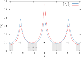
Figure 1: Histogram of the local Polyakov loop phase below and above the transition temperature and the definition of sector numbers according to Eq. 7

Below $T_{c}$, all three sectors are (almost) equally represented, giving rise to a cancellation and an (almost) vanishing average Polyakov loop $P$. This is visualized in Fig. 1, where the histogram of the local phase $\theta(x)=\arg L(x)$ is shown for a typical low-temperature configuration. For temperatures above $T_{c}$, the real sector $\theta\approx 0$ becomes dominant (also included in Fig. 1) and induces a large real average Polyakov loop. This picture of center clusters has been studied in pure gauge theory with two Fortunato and Satz (2000); Fortunato (2000), with three Gattringer (2010); Gattringer and Schmidt (2011); Endrődi et al. (2014) and with four colors Dirnberger et al. (2012), while preliminary results for dynamical quarks have been obtained in Refs. Borsányi et al. (2011); Danzer et al. (2010). (For visualisations of the clusters, see Refs. Schadler et al. (2014); Stokes et al. (2013).) We mention that while the change in the distribution of $\arg L(x)$ is essential for the deconfinement transition, the modulus $|L(x)|$ was found to play no relevant role in this respect Fortunato and Satz (2000); Fortunato (2000); Gattringer (2010); Gattringer and Schmidt (2011); Dirnberger et al. (2012); Borsányi et al. (2011); Danzer et al. (2010); Schadler et al. (2014).

Besides the distinct population of the three sectors below and above $T_{c}$, there is another pronounced difference between the confined and deconfined regimes. While the clusters are small below $T_{c}$, they percolate and span across the total volume above the transition region. In this sense the deconfinement transition becomes very similar to the percolation phenomenon in a three-state spin system. To give the center clusters a precise definition that conforms to this picture, we need to impose a filter on the local phases $\theta(x)$ that discards sites lying far from center elements. Specifically, to each site $x$ we assign a sector number $n(x)\in\{-1,0,1\}$ in the following manner Gattringer (2010):

$$n(x)=\left\{\begin{array}[]{rlrcl}+1&\mathrm{for}&\theta\in[\phantom{-}\frac{\pi}{3}+\delta\ ,\phantom{-}\pi-\delta],\\ 0&\mathrm{for}&\theta\in[-\frac{\pi}{3}+\delta\ ,\phantom{-}\frac{\pi}{3}-\delta],\\ -1&\mathrm{for}&\theta\in[-\pi+\delta\ ,-\frac{\pi}{3}-\delta],\end{array}\right.\quad\delta=\frac{\pi}{3}\cdot f.$$ (7)

Here, $f\in[0,1)$ is a free parameter, which removes “undecided” sites, i.e., those that lie close to the minima of the distribution $H(\theta)$, see Fig. 1. In the following we will refer to $f$ as the cut parameter. The center clusters are then constructed in the following way: two neighboring sites $x$ and $y$ belong to the same cluster if their sector numbers are the same, that is, if $n(x)=n(y)$. This divides space into domains where the local Polyakov loop points towards one of the three center elements.

We emphasize that a nonzero cut parameter is necessary to interpret the deconfinement transition as a percolation phenomenon. Indeed, at $f=0$, the center clusters would percolate already at low temperatures. By introducing $f\neq 0$ and discarding sites lying far from center elements, the clusters are made thinner and percolation is delayed to set in only around $T_{c}$. This way, the confined phase exhibits clusters with finite size, while in the deconfined phase there is one percolating cluster, as was demonstrated in pure gauge theory Gattringer (2010); Gattringer and Schmidt (2011); Endrődi et al. (2014). Note that similar thinning techniques (cf. Ref. Fortuin and Kasteleyn (1972)) to reduce the cluster size are necessary in different contexts as well, e.g., for the magnetic transition in the Potts model Coniglio and Klein (1980) or for the droplet description of the Ising model Fortunato (2000).

III Results

The results presented below are based on the gauge configurations generated in Refs. Bali et al. (2012a, b, 2014); Endrődi (2015) at various values of the temperature, of the magnetic field $B$ and of the lattice spacing $a$. These ensembles have been produced using the Symanzik tree-level improved gauge action and $2+1$ flavors of stout smeared rooted staggered quarks with physical masses. Details of the simulation setup and of the algorithm can be found in Refs. Aoki et al. (2006b); Borsányi et al. (2010); Bali et al. (2012a). In the following we consider the stout smeared gauge links for calculating the local Polyakov loops.

The vacuum configurations (corresponding to $T\approx 0$, $B=0$) with several lattice spacings are used to set the cut parameter $f(a)$ in a consistent manner. At finite temperatures we consider $N_{s}^{3}\times N_{t}$ lattices and employ the fixed-$N_{t}$ approach to vary the temperature. That is to say the temperature $T=(N_{t}a)^{-1}$ is changed by tuning the lattice spacing $a$ for a fixed lattice geometry. In this approach the continuum limit corresponds to the limit $N_{t}\to\infty$ at a given temperature. The magnetic field is chosen to point in the $z$-direction and enters the simulation setup via its quantized flux,

$$\Phi=eB\cdot(aN_{s})^{2}=6\pi N_{b},\quad\quad N_{b}\in\mathbb{Z},$$ (8)

where the magnetic field is measured in units of the elementary charge $e>0$. Due to flux quantization, an interpolation of the data at fixed $N_{b}$ is necessary to obtain results as a function of $eB$. For further details on the implementation of the magnetic field see Ref. Bali et al. (2012a).

III.1 Scale setting

To set the cut parameter unambiguously additional physical input is necessary. A possible way to set $f$ is to prescribe the value that the physical radius $R$ of the largest cluster should take at low temperatures Gattringer and Schmidt (2011); Endrődi et al. (2014). For a cluster of size $s$, we define the radius $R$ by the mean squared deviation of the sites $\mathbb{r}_{i}$ in the cluster from its center of mass $\mathbb{R}_{\rm CM}$:

$$\mathbb{R}^{2}=\frac{1}{s}\sum_{i=1}^{s}(\mathbb{r}_{i}-\mathbb{R}_{\rm CM})^{2}.$$ (9)

To put this implicit prescription into practice we need to search for the value of $f$ where the largest cluster has the desired radius. This procedure is visualized in Fig. 2 for various zero-temperature lattice ensembles with different lattice spacings $a$. Reading off the intersection of the $R(f)$ curves with the prescribed radius of $R=2.5\,\frac{1}{\textmd{GeV}}=0.49\,\textmd{fm}$ determines the scaling relation $f(a)$. Note that for $f\to 1$, all sites are removed and, thus, the radius shrinks to zero, while for $f=0$, the largest cluster fills the total volume so that $R$ equals half the linear lattice size. The value $R=0.49\textmd{ fm}$ which we chose for setting $f$ corresponds to a typical hadronic size relevant for the low-temperature confined regime. Note, however, that we are free to choose different radii as well. The subsequent analysis is performed using various values $0.35\textmd{ fm}<R<0.5\textmd{ fm}$.

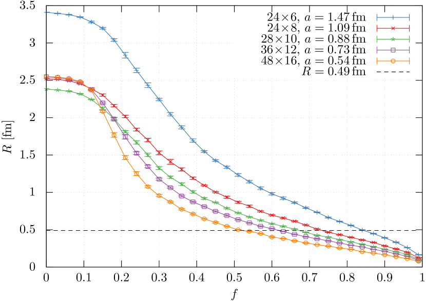
Figure 2: The radius $R$ of the largest cluster as a function of the cut parameter $f$ for our zero-temperature ensembles with various lattice spacings. The dashed line indicates the prescribed cluster radius $R=0.49\,$fm.

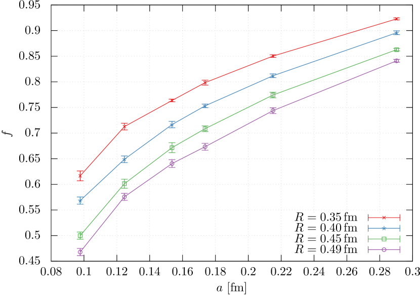
Figure 3: The cut parameter as a function of the lattice spacing for various fixed cluster radii.

The so obtained dependence $f(a)$ is shown in Fig. 3 for various values of the fixed radius $R$. The curves all have positive slopes, as expected: for finer lattices the cluster radius in lattice units $R/a$ has to be larger so that the radius in physical units $R=a\cdot R/a$ remains fixed. Thus, for smaller $a$ the clusters must be made larger (in lattice units) via decreasing $f$. In the following, the interpolation of the $f(a)$ curve will be used to set the cut parameter (for a few $N_{t}=10$ simulation points at high temperature, a controlled extrapolation is also necessary).

Having fixed the precise definition of the clusters – i.e., the dependence of the cut parameter on the lattice spacing – at $T=B=0$, we proceed to determine various properties of the clusters at nonzero temperatures and nonzero background magnetic fields.

III.2 Fractality and the mean free path

We continue the analysis by demonstrating the fractal nature of the clusters. To this end, we employ the box-counting method to define the fractal dimension $d_{\Box}$. This approach is based on the scaling

$$N(s)\propto s^{-d_{\Box}},$$ (10)

of the number $N$ of boxes of linear size $s$ necessary to cover a given cluster. This method was applied and compared to different definitions for pure gauge theory in Ref. Endrődi et al. (2014).

Fig. 4 shows the fractal dimension of the largest cluster as a function of the temperature for several different lattice spacings. At $T=113\textmd{ MeV}$, where five lattice spacings are available, the $a\to 0$ extrapolation gives $d_{\Box}=1.9(1)$ in the continuum limit. For higher temperatures we find that three lattice spacings do not suffice for a controlled continuum extrapolation of this observable.

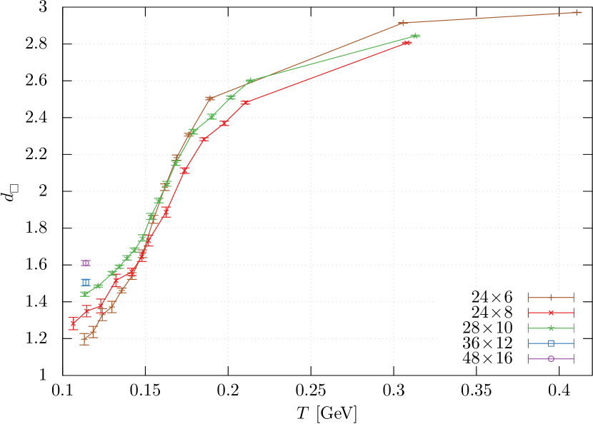
Figure 4: The fractal dimension as a function of the temperature for three lattice spacings. The zero-temperature cluster radius is fixed to $R=0.49\textmd{ fm}$.

In center cluster-based models of heavy-ion collisions a relevant parameter is the mean free path of partons inside the clusters. It is defined as the average distance that the parton can move without scattering on the cluster walls. To translate this notion into our setup, we consider the following procedure. For each site $s$ inside a cluster, we count the number $n_{s}^{i}$ of sites one can move in the direction $i$ without reaching the boundary of the cluster. The (average) mean free path is then given by

$$\lambda_{f}=\frac{1}{3}\sum\limits_{i=x,y,z}\lambda_{f}^{(i)},\quad\quad\lambda_{f}^{(i)} =\frac{1}{S}\,\sum_{s=1}^{S}\;n_{s}^{i}\cdot a,$$ (11)

where $S$ is the total number of sites available for the clusters.

Above we have seen that the clusters are not three-dimensional objects but fractals. In the pure gauge theory setting it was pointed out already in Ref. Endrődi et al. (2014) that as a consequence of this fractality the mean free path is not related to the linear cluster size but is much smaller than that. Using a continuum extrapolation based on three different lattice spacings, we show that $\lambda_{f}$ is consistent with zero for $T\lesssim 300\textmd{ MeV}$ in the continuum limit, see Fig. 5. The systematic error of the continuum extrapolation is estimated by comparing fits with different forms for the $T$- and $N_{t}$-dependence of $\lambda_{f}$. On a finite lattice, the fractal pattern is not resolved on distances smaller than the lattice spacing, thus the mean free path is bounded from below by $a$. Indeed, Fig. 5 reveals how the finite $N_{t}$ results for $\lambda_{f}$ approach zero via nonzero values. Note that as the temperature is increased further at fixed lattice spacing $a$, and the largest cluster becomes three-dimensional, $\lambda_{f}$ will approach half the linear lattice size (i.e., it will diverge in the infinite volume limit).

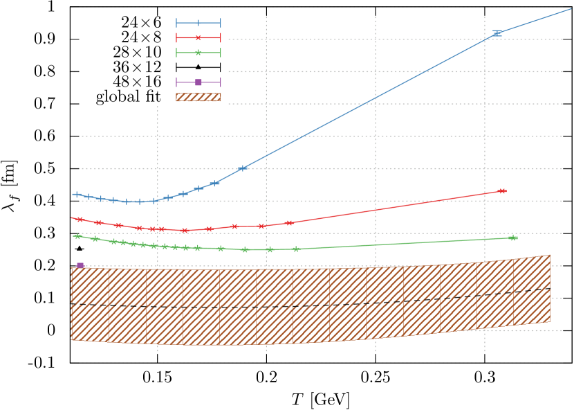
Figure 5: The mean free path as a function of the temperature, for three lattice spacings and a continuum extrapolation.

The background magnetic field breaks rotational symmetry and thus might induce an anisotropy in the directional mean free paths $\lambda_{f}^{(i)}$, defined in Eq. (11). The effect of $B$ on the Polyakov loop (and, thus, on center clusters) is indirect and occurs through virtual quark loops. In strong magnetic fields these virtual quarks occupy Landau-levels: they are free to move parallel to the magnetic field but are localized perpendicular to it. This anisotropy is expected to propagate in the gluonic sector and appear in the orientation of center clusters as well, implying $\lambda_{f}^{(z)}>\lambda_{f}^{(x)}=\lambda_{f}^{(y)}$. Another argument supporting this hierarchy is based on the finding Bonati et al. (2014) that the magnetic field reduces the string tension in the parallel but increases it in the perpendicular direction. Indeed, a reduced string tension implies enhanced correlations between distant Polyakov loops and, thus, an increased mean free path in a given direction. Interestingly, in the asymptotically strong magnetic field limit of QCD Miransky and Shovkovy (2002) the parallel string tension even vanishes and local Polyakov loops are independent of $z$ Endrődi (2015). Therefore, in this limit center clusters become tubes in the $z$-direction but are expected to retain their fractal nature in the $x-y$ plane. Nevertheless, our largest available magnetic field $eB=3.25\,\textmd{GeV}^{2}$ is still well below this asymptotic limit.

To determine whether the predicted anisotropy is present in the center structure we calculated the directional mean free paths at $eB=3.25\,\textmd{GeV}^{2}$. In accordance with the above expectation we observe $\lambda_{f}^{(z)}$ to exceed the perpendicular mean free paths, although only by a few percent. For lower magnetic fields $0<eB<0.7\,\textmd{GeV}^{2}$ the effect is found to be smaller than our statistical errors. In this range the main effect of the magnetic field turned out to be described by a shift of the transition region towards lower temperatures. We discuss this effect in more detail in the next section.

III.3 The QCD phase diagram

Due to the crossover nature of the deconfinement transition in full QCD, the observables sensitive to the transition exhibit no singular behavior but are instead smooth functions of the temperature. An implication of this is that the transition temperature is not uniquely defined: different definitions may result in different values for $T_{c}$.

The most straightforward definition involves the inflection point of the average Polyakov loop. However, this turns out to be numerically difficult to locate due to the slow and gradual rise of $P$ with the temperature, cf. Ref. Bruckmann et al. (2013). There have been proposals to circumvent this issue by considering, e.g., ratios of Polyakov loop susceptibilities that take well-defined values both well above and well below $T_{c}$, see Ref. Lo et al. (2013).

Here we propose a new method to define $T_{c}$ using center clusters. In terms of the center structure, the most substantial difference between the confined/deconfined regimes is the absence/presence of percolating clusters. (A cluster is defined to be percolating if it spans across the lattice in at least one spatial direction. Thus, such clusters become infinitely large in the infinite volume limit.) The simplest choice reflecting the abrupt change of gluonic configurations in this respect is the percolation probability $p_{\infty}$ Endrődi et al. (2014); Gattringer (2010); Dirnberger et al. (2012); Borsányi et al. (2011); Danzer et al. (2010). It is defined as the probability of having a percolating cluster and is thus bounded as $0\leq p_{\infty}\leq 1$. In Fig. 6 we plot $p_{\infty}$ as measured on the $24^{3}\times 6$ lattices, showing the expected rapid increase around $T_{c}$.

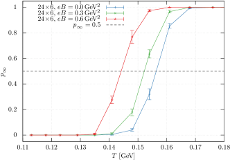
Figure 6: The percolation probability as a function of the temperature for three different values of the magnetic field. The zero-temperature cluster radius is fixed to $R=0.4\textmd{ fm}$.

Taking into account the limiting values of $p_{\infty}$ at low and at high temperatures, respectively, the most convenient choice for defining $T_{c}$ is through the implicit equation

$$p_{\infty}(T_{c}) =0.5.$$ (12)

This definition will be employed below to map out the phase diagram for nonzero magnetic fields.

To demonstrate the effect of magnetic fields on $p_{\infty}$, Fig. 6 also includes the percolation probability for a few nonzero values of $B$. Clearly, the magnetic field increases $p_{\infty}$ for all temperatures and, as a result, reduces the transition temperature. This is consistent with previous determinations of $T_{c}(B)$ using chiral quantities Bali et al. (2012a). To quantify this effect, we employed the definition (12) to determine $T_{c}$ for a range of magnetic fields using three lattice ensembles with $N_{t}=6$, $8$ and $10$. Fig. 7 shows the so obtained $T_{c}(B)$, revealing that the results for all three lattice spacings fall on top of each other. The transition temperature is found to decrease by about $10\%$ up to $eB=0.75\textmd{ GeV}^{2}$.

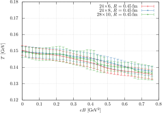
Figure 7: The transition temperature, defined according to Eq. (12), as a function of the magnetic field for three different lattice spacings. The zero-temperature cluster radius is fixed to $R=0.45\textmd{ fm}$.

Above, the cut parameter was set by fixing the zero-temperature cluster radius to $R=0.45\textmd{ fm}$. Also it is of interest how the results change if $R$ is varied. We have performed the same analysis for different values of $R$. Fig. 8 shows the continuum extrapolated transition temperatures based on our three lattice spacings for three values of the cluster radius, $R=0.40\,$fm, $R=0.45\,$fm, and $R=0.49\,$fm. The net effect of decreasing $R$ is to shift the transition temperature up. This is to be expected: the smaller the low-temperature clusters are, the stronger ordering in the local Polyakov loops (i.e., the higher temperature) is necessary for percolation to set in. Notice that $R$ affects $T_{c}$ because of the crossover nature of the transition, i.e., because the percolation probability depends smoothly on the temperature (even in the infinite volume limit). The gradual enhancement of $p_{\infty}(T)$ around $T_{c}$ becomes a real jump in pure gauge theory Endrődi et al. (2014), where the transition is of first order. In the latter case, the clusters start to percolate suddenly, so that finite changes in the low-temperature cluster radius $R$ are not expected to affect $T_{c}$. Therefore, the change in $T_{c}$ due to varying $R$ gives a measure for the width (strength) of the deconfinement transition.

It has recently been shown that the QCD phase diagram exhibits a critical endpoint for extremely strong magnetic fields Endrődi (2015), where the crossover turns into a first order transition (see also Ref. Cohen and Yamamoto (2014)). Fig. 8 also shows $T_{c}$ at a very large magnetic field for the three low-temperature cluster radii. A further decrease in $T_{c}$ by about 20% can be observed, again in agreement with previous findings based on other observables Endrődi (2015). Moreover, the difference between the $T_{c}$ curves for the different radii decreases by about 50% from $eB=0$ to $eB\approx 3.25\,\mathrm{GeV}^{2}$. According to our reasoning above this shows that the transition becomes stronger as the magnetic field grows and the predicted critical point is approached.

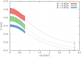
Figure 8: Continuum extrapolated transition temperatures as a function of the magnetic field for different zero-temperature cluster radii $R$. (The last three points on the far right are not continuum extrapolated but were obtained on our $N_{t}=16$ ensemble.)

IV Conclusions

In this paper we have presented first continuum extrapolated results for various observables related to the center structure of full dynamical QCD. Center clusters were identified using a consistent thinning technique involving one parameter (the cut parameter $f$) that is fixed by prescribing the cluster radius $R$ at low temperatures.

Using this prescription, the fractal dimension of the center clusters was shown to be significantly smaller than three. We demonstrated that this leads to a vanishing mean free path in the cluster structure over the range of temperatures $110\textmd{ MeV}<T<300\textmd{ MeV}$. We found that the presence of magnetic fields $eB\lesssim 3.25\textmd{ GeV}^{2}$ does not change this result qualitatively – even at our strongest magnetic field the anisotropy in the cluster orientation remains below a few percent. Thus, for a broad range of temperatures and magnetic fields that are relevant for heavy-ion collision phenomenology, the continuum extrapolated mean free path vanishes. This finding suggests a limited applicability for models that build on a finite mean free path for scattering processes in the QGP.

Furthermore, we proposed a method to define $T_{c}$ in full QCD using the percolation probability and employed this definition to determine the phase diagram for nonzero background magnetic fields. The results unambiguously show a reduction of $T_{c}$ with increasing $B$, in good agreement with the results obtained using other QCD observables Bali et al. (2012a); Endrődi (2015). In addition, the variation of $T_{c}$ when changing the zero-temperature cluster radius $R$ was argued to measure the width of the crossover transition. This quantity was found to gradually decrease as $B$ grows and the predicted critical endpoint at extremely strong magnetic fields is approached. Altogether, our findings demonstrate that the deconfinement transition in full three-color QCD can be described as a percolation phenomenon. The analysis of further observables and the discussion of finite volume effects will be performed in a forthcoming study Borsányi et al. . Finally, we note that generalizations of the percolation picture to other gauge groups, e.g., $\mathrm{SU}(N)$ with $N>3$, are non-trivial, and that more extensive research is required to adress their viability.