Spatial structures in a simple model of population dynamics for parasite-host interactions

Abstract

Spatial patterning can be crucially important for understanding the behavior of interacting populations. Here we investigate a simple model of parasite and host populations in which parasites are random walkers that must come into contact with a host in order to reproduce. We focus on the spatial arrangement of parasites around a single host, and we derive using analytics and numerical simulations the necessary conditions placed on the parasite fecundity and lifetime for the population s long-term survival. We also show that the parasite population can be pushed to extinction by a large drift velocity, but, counterintuitively, a small drift velocity generally increases the parasite population.

1 Introduction

The dynamics of coupled populations have been long studied and the topic continues to generate much interest from nearly all branches of science as a result of the broad applications it offers – from foxes and rabbits to forest fires, from chemical kinetics to disease control. This interest is sustained partly by innovations in analytical and computational tools, and by the recognition of the crucial roles played by population discreteness and various spatial inhomogeneities. Accounting for these aspects leads to surprising complexity in the population behavior [1, 2, 3, 4]. Such effects are usually studied within the context of the classical predator and prey models introduced by Lotka and Volterra [5, 6], in which the survival of each of two competing populations depends directly on its interaction with the other. This paradigm, however, represents only one of many types of inter-species interactions. Other types of interactions include symbiosis, competition, and coexistence, all of which abound in ecological and biological environments. While an ultimate goal of ecological models is an understanding of the co-evolution of a web of species [7, 8, 9, 10], our focus here is modest: the parasite-host (PH) type of interaction, inspired by flea infestation of household pets.

The main distinction of PH interactions is that the two species do not compete for survival. Instead, parasites reproduce only in the presence of a host which provides nutrients and breeding ground. Of course, parasites generally do not kill the host, so as to continue flourishing without having to find another host. Apart from fleas and pets, other examples of such interactions in nature include brood parasitism in birds, blood-sucking parasites in mammals and certain types of viruses at the cellular level. We also note that intrinsically similar models have been proposed to study topics as diverse as self-catalyzing reaction-diffusion systems [11] and economic growth centers [12]. PH interactions have been specifically investigated in [13, 14], where the system is filled with a uniform distribution of hosts before the reactions with the parasites take place. By contrast, we focus on a single host, stationary or moving uniformly, and study the spatial distribution of parasites around the host. Systems with multiple hosts have been considered previously [15], but will be mentioned only in passing.

Our model consists of a host and parasites of constant death rate. Parasites must come into contact with the host for reproduction. Typically, the life span of the parasites is much shorter than that of the host, so we consider only the birth-death process of the former, letting our hosts be simply immortal. In general, both species are mobile and their actions may depend on the location of the others. For simplicity, we will begin with a single stationary host, while allowing the parasites to perform only random walks. In the language of statistical mechanics models, this PH model belongs to the class of contact processes [16], in which the spatial structure of each population is expected to play significant roles. In our study, the only interesting spatial structure is that associated with the parasites and we show that this structure is intimately linked to the total population, $N_{\text{tot}}$. In particular, we discover that, contrary to expectations, $N_{\text{tot}}$ does not monotonically decrease when the host moves. Formulating this system on a discrete lattice, we solve this problem analytically, with results that agree well with simulations. The non-monotonicity of $N_{\text{tot}}$ can be traced to the interplay between the biased random walk and the finite carrying capacity of the host.

In the next section, we define the discrete, stochastic model in detail, providing a scheme for simulations. We then devote the following section to exact theoretical and Monte Carlo simulation results for the parasite population and distribution. In addition to the analytic solutions, we also offer some physical insights, using a continuum approximation and heuristic arguments. In particular, we note that the spatial distribution of parasite takes the same form as, say, a “pion cloud” around a nucleon. Finally we provide a summary and outlook for interesting unsolved problems, as well as extensions of this model to more realistic behavior of the hosts and the co-evolution of the two populations.

2 Parasite-host model definition

We consider an $L^{d}$ hyper-cubic lattice with periodic boundary conditions. Each of its lattice cells, labeled by an integer-valued vector $\vec{r}$, may be occupied by any number of non-interacting parasites. The number in a cell at time $t$ is denoted by $N(\vec{r},t)$. At each time step, each flea dies with probability $\mu$. The surviving ones then jump to a randomly chosen nearest neighbor cell. In our system, there is just a single immortal host located at $\vec{r}_{\text{h}}$. For each parasite in that cell, we introduce $B$ new ones and randomly place them in the neighboring cells. Here, $B$ is the integer part of

$$F\cdot V[N(\vec{r}_{\text{h}},t)]$$ (1)

where $F$ is the fecundity and $V[N(\vec{r}_{\text{h}},t)]$, a general Verhulst factor, models an environment with finite resources and depends on the parasite density at $\vec{r}_{\text{h}}$. For simplicity, we will consider only $V$’s which depend on $N/K$, where $K$ models the host carrying capacity. One consequence is that $K$ plays the role of setting an overall scale for $N$, and does not enter the general behavior (e.g., extinction) of the population. To give $F$ a sensible meaning, we will impose $V(0)=1$ so that each parasite produces $F$ offsprings in the limit of $N\ll K$. Although we can analyze the model with any $V$, here, for a variety of reasons [17], we use

$$V[N]=e^{-N/K}.$$ (2)

Note that the effective Malthusian growth per time step is not just $F-\mu$, since death occurs everywhere but birth only takes place at $\vec{r}_{\text{h}}$.

For sufficiently large $F$, we expect a steady population of parasites: the active state. If there is a single stationary host located at $\vec{r}_{\text{h}}=\vec{0}$, the ensemble average of $N(\vec{r},t)$ will approach a stationary distribution, $\rho^{\ast}(\vec{r})$. For a finite system with $\mu>0$, there is a finite probability of parasite extinction. Since that is an absorbing state, $\rho^{\ast}\equiv 0$ is the true stationary state. In this sense, we mean a quasi-stationary state when we speak of an active steady state.

For a non-stationary host, we find more interesting phenomena [15]: however, analytic understanding is challenging. We focus on a host moving with constant velocity along one of the lattice axes (say, $\hat{x}$): $\vec{r}_{\text{h}}=vt\hat{x}$. Intuitively, one expects the moving host can outrun the parasites, so that, for large enough $v$, the latter goes extinct. This picture raises the following questions: Does the parasite population always decrease with increasing $v$? If so, what is the critical $v$ for parasite extinction?

While it is easy to carry out simulations of this model, the analysis is less simple. Thus, we turn to a similar system: a stationary host with drifting parasites. In this case, the parasites perform random walk with a bias $\varepsilon$ and hops to a neighboring cell in direction $\hat{n}$, with probability

$$\frac{1-(\hat{n}\cdot\hat{x})\varepsilon}{2d}.$$ (3)

The statistical properties of this system should be the same, under a proper Galilean transformation, as those of a host moving with velocity $\propto\varepsilon\hat{x}$ in a sea of diffusing parasites with no drift. Unlike the moving host problem, the analysis of drifting parasites is straightforward and, as will be presented, simulations of both systems show that the differences are indeed minor.

Without loss of generality, we choose $\varepsilon>0$, i.e., the parasites favoring the $-x$ direction, corresponding to the host moving along $+x$ with constant velocity $\vec{v}=(v,\vec{0})$, the second entry representing transverse direction. Adopting this notation for the rest of this article, we write $\vec{r}=(x,\vec{y})$, and put the host at $(0,\vec{0})$. We implement our agent-based simulations on an $L\times L$ lattice with periodic boundary conditions. For convenience, we choose odd $L$, so that the host is placed at the center. Although we studied various lattice sizes, we present mainly the results with $L=101$, as they provide an adequate picture of the general system. With one parasite in each cell initially, we implement each Monte Carlo step (MCS) as updating each parasite, removing it with probability $\mu$ and moving each survivor to one of its $2d$ nearest neighbor cells with probability given by eq.(3). Measuring $N_{0}$, the number at the origin, we generate $B$ offsprings according to eqs.(1,2) and place each in a randomly chosen nearest neighbor cell. In most simulations, we choose $K=100$ to provide good statistics and to avoid the absorbing state. We discard the first $10^{5}$ MCS to allow the system to reach steady state. We then measure $N(\vec{r})$ for $4\times 10^{5}$ MCS after all offsprings are placed and before the next culling step. The results are used to compile averages at each cell to arrive at the stationary distribution $\rho^{\ast}(\vec{r})$.

For the moving host case, the parasites are updated as above with $\varepsilon=0$. At the end of the reproductive cycle but before the culling steps, we introduce a probability $p$, with which we move the host to the next cell along $+x$. Thus, the host velocity is $p$ per MCS. For drifting parasite, the average change in $x$ at the end of each MCS is $-\varepsilon/d$. We compare the two systems with $p=\varepsilon/d$.

We note that the velocities introduced through these rules are limited to one lattice spacing per MCS. There are many ways to achieve any velocity. However, we do not expect further qualitatively novel behavior and will restrict ourselves to the rules given above. In the summary section, we will discuss the physical significance of the various parameters.

3 Theoretical considerations and simulation results

We first study the system with a stationary host and parasites drifting along $-\hat{x}$. We exploit a mean-field equation for the evolution of $\rho(\vec{r},t)$:

$$\rho(\vec{r},t+1)=\dfrac{1}{2d}\sum_{\vec{a}}\rho(x,\vec{y}+\vec{a},t)\left[\lambda+B\delta(x)\delta(\vec{y}+\vec{a})\right]$$ (4)

$$+\dfrac{1}{2d}\sum_{\tau=\pm 1}\rho(x+\tau,\vec{y},t)\left[\lambda(1+\tau\varepsilon)+B\delta(x+\tau)\delta(\vec{y})\right].$$

Here, $\lambda\equiv 1-\mu$ is the survival probability, $\delta$ is the Kronecker delta, and $\vec{a}$ is one of the $2(d-1)$ transverse lattice vectors: $(0,...,0,\pm 1,0,...,0)$. Although $B$ is an integer in simulations, we use it to denote the key quantity controlling the birth rate $F\cdot V=F\exp\left[-\rho_{0}/K\right]$, where

$$\rho_{0}\equiv\rho(0,\vec{0},t).$$ (5)

The right side of eq.(4) accounts for the occupation at $\vec{r}$ due to transverse hopping of the surviving parasites from neighboring cells and possible newborns. In the second term on the right side of eq.(4), the effect of the bias is incorporated. Except for the non-linear aspect implicit in $B$, solving this equation is straightforward. $B$ only depends on $\rho$ through $\rho_{0}$. Thus, these terms can also be written as $\rho_{0}B\delta(...)/2d$, so that the only non-linearity is contained in a single quantity, $\rho_{0}$.

Turning to our main interest, $\rho^{\ast}(\vec{r})$ in the steady state, we defer details of its derivation to the Appendix (which also contains the generalization to arbitrary $V$) and report the findings here. Since all of our simulations are on a $d=2$ square lattice, we will drop $d$ and write $\vec{r}=(x,y)$, etc. Using a Fourier transform and regarding the stationary $\rho_{0}^{\ast}$ as a (to-be-determined) parameter, we find:

$$\rho^{\ast}(x,y)=\rho_{0}^{\ast}BG\left(x,y;\lambda,\varepsilon\right)$$ (6)

where $G$ is essentially the lattice Green’s function for biased diffusion with dissipation on a periodic square lattice. The unknown can now be fixed: $\rho_{0}^{\ast}=\rho_{0}^{\ast}B\sigma(\lambda,\varepsilon)$, where

$$\sigma(\lambda,\varepsilon)=\sum_{k,p}\dfrac{\cos k+\cos p}{2-\lambda\left(\cos k+\cos p\right)+i\varepsilon\lambda\sin k}$$ (7)

embodies the return probability of this particular random walker. Here, $k$ and $p$ are integers $\left(1,...,L\right)$ times $2\pi/L$. $\sigma$ depends not only explicitly on the system size, survival and bias, but also implicitly on the boundary conditions. With periodic boundary conditions, $\sigma$ is, despite the presence of $\varepsilon$ in eq.(7), actually a function of $\varepsilon^{2}$. This is hardly surprising given that $\sigma$ is analytic in $\varepsilon$ and cannot depend on its sign. As expected, $\sigma$ decreases monotonically as $\varepsilon$ increases for fixed $\lambda$. In particular, $\sigma^{\prime}\equiv\partial\sigma/\partial\left(\varepsilon^{2}\right)$ is negative at $\varepsilon=0$. This, however, does not guarantee that the total parasite population shares the same behavior.

Apart from the extinction $\rho_{0}^{\ast}=0$ from $\rho_{0}^{\ast}=\rho_{0}^{\ast}B\sigma$, the non-trivial steady state is given by $B\sigma(\lambda,\varepsilon)=1$. For the special $V$ we chose, the result is

$$\rho_{0}^{\ast}=K\ln(F\sigma)$$ (8)

while the total parasite population is

$$N_{\text{tot}}=\dfrac{K}{\mu\sigma}\ln(F\sigma)$$ (9)

The survival condition is $F>F_{\text{min}}=1/\sigma(\lambda,\varepsilon)$, rather than the naive $F>\mu$. The contours in fig.1 help visualize the increasing threshold for $F_{\text{min}}$. In the appendix, we show that this condition remains valid for any $V$.

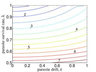
Figure 1: Contours of $F_{\text{min}}$ in the case of $L=101$ to sustain a population. For example, for $F=4$, the parasites goes extinct for $(\lambda,\varepsilon)$ below and to the right of the green contour line.

We see from eq.(9) that the bias affects $N_{\text{tot}}$ through competing factors. As a result, the sign of $\partial_{\varepsilon}N_{\text{tot}}\propto 1-\ln(F\sigma)$ can change. In particular, for $F>e/\sigma(\lambda,0)$, the parasite population first increases as $\varepsilon$ increases, reaching a maximum when $\sigma=e/F$, and then decreases to extinction at $\sigma=1/F$. For what $\varepsilon$ will $N_{\text{tot}}$ return to the unbiased value? The answer is $\tilde{\varepsilon}\left(\lambda,F\right)$, the solution to $\sigma\left(\lambda,0\right)\ln(F\sigma\left(\lambda,\tilde{\varepsilon}\right))=\sigma\left(\lambda,\tilde{\varepsilon}\right)\ln(F\sigma\left(\lambda,0\right))$. Since the population is enhanced or suppressed on either side of this line, it is instructive to show it in the $F$-$\varepsilon$ phase diagram. We illustrate in fig.2(a) the case with $\lambda=0.99$. We also display the line of maximal $N_{\text{tot}}$ defined by $\tilde{\varepsilon}$, as well as the region for extinction.

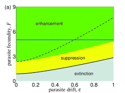
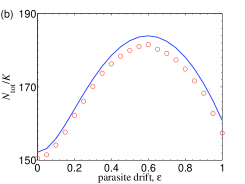
Figure 2: (a) $F-\varepsilon$ phase diagram for $\lambda=0.99,L=101$. The green/yellow areas are associated with parasite populations larger/smaller than that with no bias. Along the $F\sigma\left(\lambda,\varepsilon\right)=e$ line (dot-dashed), the population is maximal. (b) $N_{\text{tot}}(\varepsilon)/K$ for $F=5$, corresponding to traversing the solid blue line in (a), shows the competing effects of bias. The solid blue line is from eq.(9) and the symbols are results from Monte Carlo simulations. The agreement is within $\thicksim 1\%$.

In fig.2(b), we provide an example of the non-monotonic behavior corresponding to traversing the $F=5$ line (solid blue) in fig.2(a). Our simulations confirm the numerical predictions. Due to the maximum velocity imposed by our rules, the extinction phase exists only for small $F$. In the next section, we show that, for large enough $L$ and velocity, extinction prevails for any $F$ as long as $\mu>0$.

In addition to $N_{\text{tot}}$, we examine the spatial distribution of the parasites. As illustrated in fig.3, a symmetric cloud of parasites develops around the host when no bias is present. With increasing bias, the cloud is distorted, dropping sharply to the right of the host, as new parasites drift to the left. These clouds decay exponentially, an expected feature associated with death and diffusion, with two characteristic length scales as a result of the bias. In fig.4, we show integrated profiles ($\sum_{y}\rho^{\ast}(x,y)$) of these clouds. From these figures, we see an excellent agreement between simulation data and this theory.

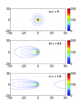
Figure 3: Countour plots of simulation data for the density profiles of the parasites with drift $\varepsilon=0,0.5$ and 1. In all cases, $F,\lambda,L=2.5,0.99,101$ and the host is located at the origin.

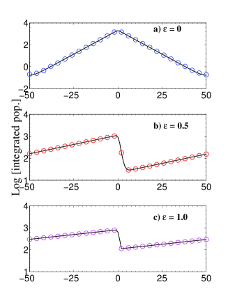
Figure 4: Integrated density profile of the parasites for both simulation (symbols) and theory (line) with $\varepsilon=0,0.5$ and 1. In all cases, $F,\lambda,L=2.5,0.99,101$. Parasites of the same horizontal coordinates are summed together.

Finally, we turn to the case of a moving host with a population of unbiased parasites. The full stochastic process can be written and, naively, there should be no difference between this process and the one above after a Galilean transformation. To compare the two, we show the integrated density profiles for a typical case ($F,\lambda,L=2.5,0.99,101$) with $\varepsilon=0.5$ and $p=\varepsilon/2$ in fig.5. The average overall properties of the two system are indeed very similar. While the moving host problem may be analytically solvable, this result lessens the urgency for such a pursuit.

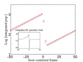
Figure 5: Comparison between the integrated density profiles for drifting parasites (red $\circ$) and moving host ($\times$). Inset gives the absolute difference between the two cases with $F,\lambda,L=2.5,0.99,101$.

4 Insights from the continuum limit

To gain more intuitive physical insight, we consider the continuum and thermodynamic limits. Here, $\vec{r}$ is taken to be continuous and $\rho(\vec{r})$ is the parasite number density. We can write $\partial_{t}\rho=\left[D\nabla^{2}-u\partial_{x}-\tau^{-1}\right]\rho$, where $D$ is the diffusion constant, $-u\hat{x}$ is the drift velocity, and $\tau$ is the average lifetime. Without drift, the characteristic length is $\xi=\sqrt{D\tau}$. We can cast the effects of the bias in a dimensionless quantity, $w\equiv u\tau/2\xi$. In the absence of a source, $\rho$ vanishes as $t\rightarrow\infty$. If we place a source of “charge” $Q$ (with units of parasite births per unit time) at the origin, then a stationary state $\rho^{\ast}(\vec{r})$ exists and satisfies:

$$\left[-\xi^{2}\nabla^{2}+2w\xi\partial_{x}+1\right]\rho^{\ast}(\vec{r})=Q\tau\delta(\vec{r})$$ (10)

We see $N_{\text{tot}}=Q\tau$ with an implicit $w$-dependence being through $Q$. Notably, for $w=0$, $\rho^{\ast}$ is the solution of the inhomogeneous Helmholtz equation and, in $d=3$, is analogous to the potential associated with the Yukawa interaction from particle physics and to the Debye-Hückel interaction from colloidal physics. The behavior far from the origin is dominated by $e^{-\left|\vec{r}\right|/\xi}$ for any $d$, while it diverges as $r^{2-d}$ near the origin for $d>2$. Unlike in typical physics problems, $Q$ here is specified by the birth rate at the host, which is determined by the return probability of a newborn to the host. This non-linear feedback produces an unusual twist to the physics of finite-ranged interactions, allowing for complex and counterintuitive effects. In particular, if there is a true “point” host, then $Q$ depends on $\rho(\vec{0})$ and we must deal with ultraviolet singularities for $d\geq 2$. The more tractable method is to introduce a cutoff, say within radius $a$, where the reproduction occurs. On the other hand, the precise shape of the reproductive region, as long as it is finite, is irrelevant for the large $\vec{r}$ behavior of $\rho$. There, the parasite cloud depends only on $\xi$ and an “effective charge” $Q_{\text{eff}}$. This approach is similar to the renormalization program in quantum and statistical field theories, where the large scale properties are universal, dependent on renormalized quantities (in this case, $Q_{\text{eff}}$ and $\xi$) and independent of other details of the microscopics. Therefore, the relationship between the details of the host and say, $N_{\text{tot}}$, is not accessible in general. Nevertheless, we illustrate an intuitive and qualitative picture using the following arguments.

We allow reproduction by the parasites that get close to the host and denote their numbers by $N_{\text{r}}$. Each gives birth at a fixed rate $\Phi$ (fecundity per unit time). We also introduce a Verhulst factor, $V(N_{\text{r}})$, a specific example being $\exp[-N_{\text{r}}/K]$. With no bias, we may assume that $N_{\text{r}}$ is the integral of $\rho$, which is $\thicksim r^{2-d}$ for small $r$, apart from logarithms in $d=2$ over a region of size $a$. We can approximate $N_{\text{r}}\thicksim N_{\text{tot}}(a/\xi)^{2}$ and write $Q=N_{\text{r}}\Phi V$. With $N_{\text{tot}}=Q\tau$, we arrive at: $N_{\text{r}}\left(a/\xi\right)^{-2}\thicksim N_{\text{r}}\Phi V(N_{\text{r}})\tau$, so that a non-trivial solution is

$$N_{\text{tot}}\thicksim K(a/\xi)^{-2}\ln\left[\Phi\tau(a/\xi)^{2}\right].$$ (11)

Comparing with eq.(9), we see that $\Phi\tau(a/\xi)^{2}$ plays the role of $F\sigma$: $\Phi\tau$ is the ratio of birth to death rates and $(a/\xi)^{2}$ is the fraction in the population that can reproduce.

Now let us look into the effects of biased diffusion. This is best revealed in the simple $d=1$ case. The parasite density profile is

$$\rho(x)=Q\tau e^{\mp x/\xi_{\pm}}/(\xi_{+}+\xi_{-})\text{~{}~{}for~{}~{}}x\gtrless 0$$

where $\xi_{+}$($\xi_{-}$) controls the tail along (against) the bias and $\xi_{\pm}=\sqrt{1+w^{2}}\pm 1$. This is similar to the integrated profiles shown in fig.4. Defining $N_{\text{r}}$ by $\int_{-a}^{a}\rho\upd x$ ($a\ll\xi_{-}$), we find it to be $1/\sqrt{1+w^{2}}$ times the non-biased case. Though this factor decreases monotonically with $w$, $N_{\text{tot}}$ can increase due to the increase in $V$. The drift reduces the parasite population at the host and, in appropriate circumstances, allows for more newborns.

5 Summary and outlook

In this article, we report studies of a simple system of non-interacting parasites, reproducing in the presence of a single host. Using a Verhulst factor for the birth rates, the population reaches a steady state at long times, with a non-trivial density profile. With a uniformly moving host, the results are essentially the same as those in a system with a stationary host and drifting parasites (executing random walks with an appropriate bias). This equivalence is fairly intuitive, since the two system are related by a Galilean transform apart from minor details in stochastic rules. It is tempting to expect that a moving host is less supportive to the parasites, so that their population would decrease with the speed. Surprisingly, our study reveals a regime of fecundity in which the total population increases with drift speed, before decreasing to extinction. We find analytic solutions valid for periodic lattices in any dimension and the agreement with simulation is excellent. We also considered a continuum version to provide a more illuminating understanding of the physical system.

In closing, let us remark on a number of interesting generalizations of our system, some of which were discovered in preliminary studies [15]. Imposing reflecting BC’s, instead of periodic BC’s, breaks translational invariance and leads to novel features: the system supports a larger parasite population when the host is placed near a wall or a corner due to the increased return probabilities of the newborns. An alternative perspective is that the “image charge” of the host is closer when it is near a wall or corner. Similar cooperative behavior emerges when there are $M>1$ hosts: the total parasite population is more than the sum of the individual cases. As long as the hosts are stationary, we can extend our analytic results.

More interesting properties appear if the host moves, either randomly or with deference to the gradient of local parasite densities. With reflecting BC’s, it is equally likely to find the host anywhere in the former case and more likely to find it near the center for the latter. Meanwhile, the parasite profile peaks at the corners and the center in the two cases, respectively. The details also depend on the relative hopping rates, in addition to competing factors like $\mu$ and $L$. Adding more smart hosts raises the natural issue of mutual avoidance. If we probe the trajectories of these hosts, we should find “scattering” events because their effective interaction is repulsive, mediated by the respective parasite clouds. A systematic exploration, which may reveal other novel phenomena, should be undertaken. Here, we limited ourselves to populations with relatively low birth rates, so that the systems relax into stable steady-states. Regarding our system in the same light as the logistic map, $x_{n+1}=\lambda x_{n}(1-x_{n})$, we expect, for very high birth rates, to encounter instability, possibly transitioning to bifurcation and chaos. Beyond this PH system, we can consider multiple species with various forms of interdependence, which could pave the way to the study of more complex and realistic food-webs.

6 Appendix: Solution for the steady state in a finite discrete lattice

We present the essentials to derive the stationary solution for eq.(4). Writing $\tilde{\rho}^{\ast}(k,\vec{p})=\sum_{\vec{r}}e^{ikx+i\vec{p}\cdot\vec{y}}\rho^{\ast}(\vec{r})$ and carrying out the sum on both sides of eq.(4), we find

$$\tilde{\rho}^{\ast}(k,\vec{p})=\rho_{0}^{\ast}B\frac{A(k,\vec{p})}{d-\lambda A(k,\vec{p})+i\varepsilon\lambda\sin k},$$ (12)

where $A(k,\vec{p})=\cos k+\sum_{i=2}^{d}\cos p_{i}$. Inserting this into the inverse transform, $\rho^{\ast}(\vec{r})=\sum_{k,\vec{p}}e^{-ikx-i\vec{p}\cdot\vec{y}}\tilde{\rho}^{\ast}(\vec{k})$, where $\sum_{k,\vec{p}}$ denotes summing over integer ($1,...,L$) multiples of $2\pi/L$ with a factor of $L^{-d}$, we find eq.(6) with

$$G(x,\vec{y};\lambda,\varepsilon)=\sum_{k,\vec{p}}\frac{A(k,\vec{p})}{d-\lambda A(k,\vec{p})+i\varepsilon\lambda\sin k}e^{-ikx-i\vec{p}\cdot\vec{y}}.$$ (13)

For self consistency, the unknown $\rho_{0}^{\ast}$ must satisfy $\rho_{0}^{\ast}\equiv\rho^{\ast}(0,\vec{0})=\rho_{0}^{\ast}BG(0,\vec{0};\lambda,\varepsilon)$, the $d=2$ version being eq.(7). Finally, the total population is

$$N_{\text{tot}}=\sum_{\vec{r}}\rho^{\ast}(\vec{r})=\tilde{\rho}^{\ast}(\vec{0})=\frac{\rho_{0}^{\ast}B}{1-\lambda}=\frac{\rho_{0}^{\ast}}{\mu\sigma}.$$ (14)

It is easy to generalize these results to arbitrary $V$’s that depend on $\rho$ through $\phi\equiv\rho/K$. The non-trivial stationary condition then reads $V(\phi_{0}^{\ast})=1/(F\sigma)$ , while $N_{\text{tot}}=\phi_{0}^{\ast}(K/\mu\sigma)=(FK/\mu)\phi_{0}^{\ast}V(\phi_{0}^{\ast})$. Extinction is given by $F\sigma=1/V(0)=1$, while the maximum of $N_{\text{tot}}$ occurs at $\tilde{\phi}_{0}^{\ast}$, which satisfies $\tilde{\phi}_{0}^{\ast}=-\left.\partial\ln V\right|_{\tilde{\phi}_{0}^{\ast}}$ and translates to a line in the $(\lambda,\varepsilon)$ plane through $1/\sigma(\lambda,\varepsilon)=FV(\tilde{\phi}_{0}^{\ast})$.

- [1] \NameNelson D. R. Shnerb N. M. \REVIEWPhys. Rev. E5819981383.
- [2] \NameReichenbach T., Mobilia M. Frey E. \REVIEWPhys. Rev. E742006051907.
- [3] \NameParker M. Kamenev A. \REVIEWPhys. Rev. E802009021129.
- [4] \NameKorolev K. S., Avlund M., Hallatschek O. Nelson D. R. \REVIEWRev. Mod. Phys.8220101691.
- [5] \NameLotka A. J. \REVIEWJournal of the american chemical society4219201595.
- [6] \NameVolterra V. \REVIEWNature1181926558.
- [7] \NameMode C. J. \REVIEWEvolution121958158.
- [8] \NameAnderson R. M. May R. M. \REVIEWThe Journal of Animal Ecology471978219.
- [9] \NameMay R. M. Anderson R. M. \REVIEWThe Journal of Animal Ecology471978249.
- [10] \NameMcKane A. J. Drossel B. \REVIEWEcological Networks: Linking Structure to Dynamics in Food Webs. Oxford University Press, Oxford2006223.
- [11] \NameTogashi Y. Kaneko K. \REVIEWPhys. Rev. E702004020901.
- [12] \NameYaari G., Nowak A., Rakocy K. Solomon S. \REVIEWThe European Physical Journal B622008505.
- [13] \NameShnerb N. M., Louzoun Y., Bettelheim E. Solomon S. \REVIEWProceedings of the National Academy of Sciences97200010322.
- [14] \NameLouzoun Y., Solomon S., Atlan H. Cohen I. \REVIEWBulletin of Mathematical Biology652003375.
- [15] \NameSkinner B., Schmittmann B. Zia R. K. P. \REVIEWunpublished2004.
- [16] \NameMarro J. Dickman R. \BookNonequilibrium phase transitions in lattice models (Cambridge University Press) 2005.
- [17] \NameRicker W. E. \REVIEWJournal of the Fisheries Research Board of Canada111954559.