Double-jump stochastic volatility model for VIX: evidence from VVIX

Double-jump stochastic volatility model for VIX: evidence from VVIX

Abstract

The paper studies the continuous-time dynamics of VIX with stochastic volatility and jumps in VIX and volatility. Built on the general parametric affine model with stochastic volatility and jump in logarithm of VIX, we derive a linear relation between the stochastic volatility factor and VVIX index. We detect the existence of co-jump of VIX and VVIX and put forward a double-jump stochastic volatility model for VIX through its joint property with VVIX. With VVIX index as a proxy for the stochastic volatility, we use MCMC method to estimate the dynamics of VIX. Comparing nested models on VIX, we show the jump in VIX and the volatility factor is statistically significant. The jump intensity is also state-dependent. We analyze the impact of jump factor on the VIX dynamics.

Keywords: Volatility indices, Volatility proxy, Co-jump, Monte Carlo Markov chain, Bayesian analysis

1 Introduction

Modelling VIX index and its derivatives has been a hot topic among researchers. As a measure for market’s expectation of 30-day implied volatility of S&P500 index, VIX provides rich information for the prediction of market’s future trend. It can be seen as a compression of information involved in S&P500 options. Usually, the VIX and S&P500 index have an empirical negative correlation relationship, so VIX index is often referred to as the fear index or the fear gauge. For more about VIX, see e.g. Carr and Wu (2005).

Out of its importance, much attention has been focused on modelling the dynamics of VIX directly. Earlier work tries using geometric Brownian motion, square root diffusion or log-normal Ornstein-Uhlenbeck (OU) diffusion to model VIX. Jumps in VIX are also added by some authors. Recently, a novel parameterized stochastic volatility model for VIX is put forward by Mencia and Sentana (2013) and Kaeck and Alexander (2013). They specify a new process to model the volatility of VIX which may be correlated with VIX and show its empirical advantage over the other traditional models. Both of them also point out that the appearance of this stochastic volatility reduces the impact of jump on VIX. However, the model specification of this novel stochastic volatility diverges between them. Mencia and Sentana (2013) adopt a pure-jump OU process out of the analytical treatability while Kaeck and Alexander (2013) characterize the volatility as a square root diffusion which takes the correlation of the volatility and VIX into account. How to specify and estimate this volatility factor and further interpret the dynamics of VIX better is still an open problem.

In 2012 CBOE introduces a new volatility index named VVIX into market. Like the role of VIX, VVIX measures the 30-day implied volatility of VIX index. Huang and Shaliastovich (2014) construct the realized volatility of VIX index (i.e. realized volatility of volatility) and show that the VIX index itself is not a good predictor for its realized volatility while VVIX serves as a better candidate. We thus can infer from their empirical conclusion that the VVIX index may provide some extra information about the volatility of VIX beyond the VIX itself.

In this paper we mainly study the dynamics of VIX and especially concentrate on modelling its stochastic volatility under the physical measure via additional information provided from VVIX index. Based on joint behavior of VIX and VVIX we put forward a double-jump stochastic volatility model for logVIX and its volatility. We will show that under a general affine assumption for the logarithm of VIX and its stochastic volatility, the stochastic volatility and VVIX satisfy a linear relationship, then the property of this stochastic volatility follows from VVIX naturally. This relation can be seen as a benchmark to see whether the estimated stochastic volatility factor is accurate enough and also provide the empirical evidence for its model specification. From the historical data of VIX and VVIX, we find both of them are mean-reverting. Furthermore, through a formal test we find there exists evident co-jump between them. Thus we conduct an empirical analysis of the double-jump stochastic volatility model and its nested models using Markov-Chain-Monte-Carlo (MCMC) method with historical data of VIX and VVIX. We provide evidence consistent with jumps in both VIX and the volatility and that jump intensity is stochastic. We demonstrate the superiority of our main model through residual analysis and simulation result.

The structure of this paper is as follows: Section 2 reviews the related literature. Section 3 shows the linear relationship between VVIX index and the stochastic volatility. Section 4 analyzes model specification and sets ip our model. Section 5 gives our empirical method. Section 6 describes the data of VIX and VVIX that we use in this paper. Section 7 summarizes the estimation results and provide empirical analysis. Section 8 concludes.

2 Literature review

To build a parameterized stochastic model for VIX, there are usually two different starting points. One is first modelling a multi-factor stochastic volatility process for S&P500 index and then derive a calculating formula for VIX index under this circumstance. For more about multi-factor model setup, see e.g. Duffie et al. (2000), Gatheral (2008), Egloff et al. (2010), Cont and Kokholm (2013) and Papanicolaou and Sircar (2014). From the model assumption, the final VIX may be a combination of one or more factors (see e.g. Ait-Sahalia et al. (2014), Song and Xiu (2012), Luo and Zhang (2012), Lin and Chang (2009)). The other method is to model VIX index directly which often has mean-reverting property. In this case, there are usually two ways to deal with the dynamics of VIX: affine and non-affine (see e.g. Mencia and Sentana (2013), Kaeck and Alexander (2013), Goard and Mazur (2013)). In the catalogue of non-affine models, modelling logarithm of VIX directly is most popular and has been proved empirically better than affine assumption of VIX.

Recently, modelling VIX with an additional stochastic volatility calls more attention. Along the literature, the existence of stochastic volatility in the dynamics of S&P500 has been widely proved and accepted empirically. Similarly, in terms of VIX index, the justification for stochastic volatility is also tested and verified (see e.g. Wang and Daigler (2012), Huang and Shaliastovich (2014)). Various authors has built VIX model with stochastic volatility and found the model with stochastic volatility factor outperforms the others without it. In Mencia and Sentana (2013), they make comparison of different models for VIX with VIX, VIX futures and VIX options as the data source. They use extended Kalman filter to estimate stochastic volatility and conclude that modelling logarithm of VIX with stochastic mean and stochastic volatility (named ’CTOUSV’ in their paper) is the best among all of the candidate models. In that paper, they first put forward the stochastic volatility of volatility model of VIX and model the volatility factor using pure jump OU process. Kaeck and Alexander (2013) employ VIX data of nearly 20 years to estimate the VIX models with and without stochastic volatility using MCMC method. They model the volatility factor as a square-root diffusion process and prove the stochastic volatility model fits better for the VIX historical data. Barndorff-Nielsen and Veraart (2013) derive probabilistic properties of a class of stochastic volatility of volatility models.

From Huang and Shaliastovich (2014), we conclude that using only VIX index to infer the dynamics of the stochastic volatility factor of VIX is not a good idea. At least some additional data set must be taken into consideration. In terms of estimation, the data source matters. Estimation using various data sources can produce distinct empirical results which show their different information content (see e.g. Bardgett et al. (2013), Chung et al. (2011)). In the framework of parameterized SDE model for VIX, employing VIX and its derivatives (futures and options) has been implemented before. However the formulas for VIX options are generally vey complex and usually involve inverse Fourier transform which may increase the calculation burden. Closed-form solutions are thus not easy to obtain for VIX options. In that case, expansions is a good way (see e.g. Li (2013), Xiu (2014)). The information from VIX options are in essence equivalent to their implied volatility as other variables like time to maturity and strikes are known. As a volatility index for VIX options, VVIX just serves as the role of the implied volatility of VIX. Using VVIX index to estimate dynamics of VIX is still a vacuum in the literature and we will fill this gap in our paper.

3 VVIX as a proxy for volatility of VIX

3.1 A motivation

In Kaeck and Alexander (2013), they put forward a stochastic volatility of volatility model for VIX. They assume the logarithm of VIX has a normal jump while its stochastic volatility factor satisfies a square-root diffusion model. Denote by $Y\left(t\right)$ the VIX index, we write this model under $P$,

$$dY\left(t\right) = \kappa_{V}\left(\theta-Y\left(t\right)\right)dt+\sqrt{\omega\left(t\right)}dW_{Y}^{P}\left(t\right)+J_{Y}^{P}dN\left(t\right)$$

$$d\omega\left(t\right) = \kappa_{\omega}^{P}\left(\varpi^{P}-\omega\left(t\right)\right)dt+\sigma_{\omega}\sqrt{\omega\left(t\right)}dW_{\omega}^{P}\left(t\right)$$ (1)

where $\left\langle dW_{Y}^{P}\left(t\right),dW_{\omega}^{P}\left(t\right)\right\rangle=\rho dt$. $N\left(t\right)$ is Poisson process with constant jump intensity $\lambda$,

$$J_{Y}^{P}\sim N\left(\mu_{y}^{JP},\left(\sigma_{y}^{J}\right)^{2}\right)$$

They use VIX data of 20 years as the input to estimate (1) and give the estimated latent stochastic volatility $\omega\left(t\right)$. A question arises naturally: how to guarantee and measure the accuracy of the estimation of this unobserved spot volatility? Bardgett et al. (2013) find that both of S&P500 options and VIX options contain some information that are unspanned by their counterpart. VIX is a volatility index summarized from S&P500 options while its diffusion part must reflect the implied volatility of VIX options. So employing VIX index as the only input to infer the dynamics of its stochastic volatility is doubted. While VIX options can provide wanted extra information, the computation burden rises quickly and sometimes complicated inverse Fourier transform is needed out of the complex expression of the price of VIX options. However, we will show in the next part that there exists a simple linear relationship between the stochastic volatility factor and the VVIX index which is compiled from a strip of VIX options mentioned above.

3.2 Linear relationship between VVIX and volatility of VIX

Following Mencia and Sentana (2013) and Kaeck and Alexander (2013), in this part we build model on the logarithm of VIX instead of VIX directly. We show that if logVIX mean reverts to a constant central tendency with stochastic volatility and jumps in logVIX and volatility, then there exists a linear relationship between VVIX index and this stochastic volatility factor of the logVIX. This relationship can provide a gauge to see whether a stochastic volatility model for VIX can be reliable. The similar idea of finding a proxy for some unobservable factor can also be found in Ait-Sahalia and Kimmel (2007), Duan and Yeh (2010) and Ait-Sahalia et al. (2014). In this paper, VIX index is the underlying asset so its dynamics are observed under $P$ measure. As VVIX is compiled from VIX options which is calculated under the pricing measure $Q$, all of the derivation involving VVIX below will be implemented under $Q$ measure.

Let $Y\left(t\right)=\log VIX\left(t\right)$ and assume that under $Q$, $Y\left(t\right)$ and $\omega\left(t\right)$ follow a general affine jump diffusion model

$$dY\left(t\right) = \kappa_{V}\left(\theta-Y\left(t\right)\right)dt+\sqrt{\omega\left(t\right)}dW_{Y}^{Q}\left(t\right)+J_{Y}^{Q}dN\left(t\right)$$

$$d\omega\left(t\right) = \left(\alpha_{\omega}-\kappa_{\omega}^{Q}\omega\left(t\right)\right)dt+\sigma_{\omega}\sqrt{\omega\left(t\right)}dW_{\omega}^{Q}\left(t\right)+J_{\omega}^{Q}dN\left(t\right)$$ (2)

where we assume $\left\langle dW_{Y}^{Q}\left(t\right),dW_{\omega}^{Q}\left(t\right)\right\rangle=\rho dt$. $N\left(t\right)$ is a Poisson process with stochastic jump intensity $\lambda\left(t\right)=\lambda_{0}+\lambda_{1}\omega\left(t\right)$ at time $t$ for analytical treatability. The jump for VIX and its volatility factor are characterized by

$$J_{Y}^{Q}\sim N\left(\mu_{y}^{J},\left(\sigma_{y}^{J}\right)^{2}\right)$$

$$J_{\omega}^{Q}\text{ }\char 126\relax\text{ }N\left(\mu_{\omega}^{J},\left(\sigma_{\omega}^{J}\right)^{2}\right)$$

Similar to the idea that regarding VIX square as the expectation of quadratic variation of the logarithm of the S&P500 index under the pricing measure approximately (see, e.g. Ait-Sahalia et al. (2014)), we set

$$VVIX_{t,t+\tau}^{2}=\frac{1}{\tau}\left[E_{t}^{Q}\left(\int_{t}^{t+\tau}\omega\left(s\right)ds\right)+E_{t}^{Q}\left(\sum_{s\geq 0}\bigtriangleup Y^{2}\left(s\right)\right)\right]$$ (3)

With simple calculation from (2) we obtain

$$E_{t}^{Q}\left(\int_{t}^{t+\tau}\omega\left(s\right)ds\right) = \frac{1-e^{-\left(\kappa_{\omega}^{Q}-\lambda_{1}\mu_{\omega}\right)\tau}}{\kappa_{\omega}^{Q}-\lambda_{1}\mu_{\omega}}\omega\left(t\right)+\left(\tau-\frac{1-e^{-\left(\kappa_{\omega}^{Q}-\lambda_{1}\mu_{\omega}\right)\tau}}{\kappa_{\omega}^{Q}-\lambda_{1}\mu_{\omega}}\right)\frac{\alpha_{\omega}+\lambda_{0}\mu_{\omega}}{\kappa_{\omega}^{Q}-\lambda_{1}\mu_{\omega}}$$ (4)

$$\triangleq \alpha_{Q}\omega\left(t\right)+\beta_{Q}$$

and

$$E_{t}^{Q}\left(\sum_{s\geq 0}\bigtriangleup Y^{2}\left(s\right)\right) = \left(\left(\mu_{y}\right)^{2}+\left(\sigma_{y}^{J}\right)^{2}\right)E_{t}^{Q}\left(\int_{t}^{t+\tau}\left(\lambda_{0}+\lambda_{1}\omega\left(s\right)\right)ds\right)$$ (5)

$$= \left(\left(\mu_{y}\right)^{2}+\left(\sigma_{y}^{J}\right)^{2}\right)\left(\lambda_{0}\tau+\lambda_{1}\beta_{Q}+\lambda_{1}\alpha_{Q}\omega\left(t\right)\right)$$

Combine (3), (4) and (5), we finally have

$$VVIX_{t,t+\tau}^{2} = \frac{1}{\tau}\left[\alpha_{Q}\omega\left(t\right)+\beta_{Q}+\left(\left(\mu_{y}\right)^{2}+\left(\sigma_{y}^{J}\right)^{2}\right)\left(\lambda_{0}\tau+\lambda_{1}\beta_{Q}+\lambda_{1}\alpha_{Q}\omega\left(t\right)\right)\right]$$ (6)

$$= \frac{1}{\tau}\left[\left(\beta_{Q}+\left(\left(\mu_{y}\right)^{2}+\left(\sigma_{y}^{J}\right)^{2}\right)\left(\lambda_{0}\tau+\lambda_{1}\beta_{Q}\right)\right)+\left(1+\lambda_{1}\left(\left(\mu_{y}\right)^{2}+\left(\sigma_{y}^{J}\right)^{2}\right)\right)\alpha_{Q}\omega\left(t\right)\right]$$

$$\triangleq A\left(\tau\right)+B\left(\tau\right)\omega\left(t\right)$$

Relationship (6) can be seen as a benchmark for the estimated volatility factor. The dynamics of VVIX can reflect the property of $\omega\left(t\right)$ more directly than the indirect impact of VIX option. It can provide more intuitive empirical evidence for the model specification for $\omega\left(t\right)$ which will be seen in Section 4.

3.3 Examination using the benchmark

If we define a suitable set of risk premia specification for this model to guarantee that its $Q$-counterpart remains the same structure as that under $P$, then the linear relation in Section 3.2 holds. We want to use VVIX index as a benchmark (let $J_{\omega}^{Q}=0$, $\lambda_{1}=0$) to judge whether the estimation for $\omega\left(t\right)$ from only VIX index is reliable and reflect the real evolution of the market. As the VVIX data only starts from 2007, so in this part, we use VIX data from Jan 2007 to Sep 2014 to estimate this model again using the same method as Kaeck and Alexander (2013). We plot the estimated volatility factor $\omega\left(t\right)$ and VVIX time series of the same period in Figure 2. The correlation between this posterior volatility and VVIX index is only 0.4193. Although some of the peaks of estimated $\omega\left(t\right)$ coincide with VVIX, more inconsistence between them appears. This indicates that when we use VIX index as the only data source to sample latent variable $\omega\left(t\right)$, it could only provide limited information about the dynamics of its stochastic volatility and the stochastic volatility is unspanned by the VIX in some sense. To obtain more accurate $\omega\left(t\right)$, the relationship between it and the VVIX index can be utilized.

4 Model specification and setup

4.1 Model specification

The log-normal Ornstein-Uhlenbeck model is put forward by DetempleandOsakwe(2000). Ever since, modelling the logarithm of VIX or VIX futures is considered in Psychoyios et al. (2010) and Huskaj and Nossman (2013). Mencia and Sentana (2013) and Kaeck and Alexander (2013) compare and examine different model specification for VIX dynamics. Both of them conclude that the setup for modelling logVIX as an affine jump process is superior to modelling VIX directly which is consistent among all of the model specifications in more detail. So in our model, we also study the affine property of logVIX.

Since there exists such linear relationship between VVIX and $\omega\left(t\right)$, the VVIX index can be seen as a proxy for this unobservable variable. The joint modelling of VIX index and its stochastic volatility is thus equivalent to the joint modelling for VIX index and VVIX index. In this sense, the model should reflect some of their joint property.

Both VIX and VVIX have the mean-reverting property. For VIX, it may mean revert to a constant or stochastic central tendency. In Mencia and Sentana (2013), they make both assumptions and examine the model performance respectively. As their data source consists of VIX, VIX futures and VIX options, the stochastic central tendency of VIX models performs better. In fact the specification of the central tendency of VIX is mainly characterized by the information from VIX futures while the VIX options play a relatively light role. However, from the derivation in Section 3.2 we know that the expression of VVIX index is irrelevant of the drift part of VIX. In fact, this is consistent with its stochastic volatility role. As our paper mainly concerns about the impact of VVIX data for the estimation, we make a simple assumption that the VIX mean reverts to a constant central tendency. As VVIX has the similar empirical property, we also assume the stochastic volatility of VIX has a constant central tendency.

From historical daily data of VIX and VVIX from Jan 2007 to Nov 2014, we observe that there exists evident co-jump between the two index, no matter positive or negative jump happened. To make a formal test to verify this phenomenon, we adapt the method in Bollerslev et al. (2008) to the lower sampling frequency (see also Gilder (2009) for the practice of this method for daily data). The testing procedure is divided into two steps: first, we show there exist jumps in both VIX and VVIX and second, the VIX and VVIX have common jumps.

To carry on the first step, we assume a process $X$ (to be VIX or VVIX) is observed in $\left[0,T\right]$ at daily times $t=0,1,\ldots,T$ and denote the time series by $X_{t},t=1,2,\ldots,T$. The return process $r_{t}=X_{t}-X_{t-1},t=1,2,\ldots,T$ is also defined. We compute the $n$-day rolling sample estimates of realized volatility,

$$RV_{t}=\sum\nolimits_{k=0}^{n}r_{t-k}^{2}$$ (7)

and bipower variation

$$BV_{t}=\frac{\pi}{2}\sum\nolimits_{k=0}^{n-1}\left|r_{t-k}\right|\left|r_{t-k-1}\right|$$ (8)

The relative contribution measure

$$RJ_{t}=\frac{RV_{t}-BV_{t}}{RV_{t}}$$ (9)

follows from (7) and (8) immediately. The tripower quarticity for daily changes is defined by

$$TP_{t}=\mu_{4/3}^{-3}\frac{n^{2}}{n-2}\sum\nolimits_{k=0}^{n-1}\left|r_{t-k}\right|^{4/3}\left|r_{t-k-1}\right|^{4/3}\left|r_{t-k-2}\right|^{4/3}$$ (10)

where $\mu_{4/3}=2^{2/3}\Gamma\left(\frac{7}{6}\right)\Gamma\left(\frac{1}{2}\right)$. Finally, the statistic

$$z_{t}=\frac{RJ_{t}}{\sqrt{\left[\left(\pi/2\right)^{2}+\pi-5\right]\frac{1}{n}\max\left(1,\frac{TP_{t}}{BV_{t}^{2}}\right)}}$$ (11)

is constructed using (8), (9) and (10) to test whether a jump occurs at day $t$. We reject the null hypothesis of no jumps at $\alpha\%$ confidence level if $\left|z_{t}\right|>\Phi_{1-\alpha/2}^{-1}$ where $\Phi$ is the cumulative normal distribution for a given day $t$.

To implement the second step, denote the VIX and VVIX by $X^{1}$ and $X^{2}$. Assume VIX and VVIX index are observed in $\left[0,T\right]$ at daily times $t=1,2,\ldots,T$, the time series are thus $X_{t}^{i},t=1,2,\ldots,T,i=1,2$ respectively. Given the return processes $r_{t}^{i}=X_{t}^{i}-X_{t-1}^{i},t=1,2,\ldots,T,i=1,2$, we calculate the contemporaneous correlation

$$cp_{t}=\sum\nolimits_{k=0}^{n-1}r_{t-k}^{1}r_{t-k}^{2}$$

and study the studentized statistic

$$z_{cp,t}=\frac{cp_{t}-\overline{cp}}{s_{cp}}$$ (12)

where

$$\overline{cp}=\frac{1}{T-\left(n-1\right)}\sum\nolimits_{t=n}^{T}cp_{t}$$

and

$$s_{cp}=\left[\frac{1}{T-\left(n-1\right)}\sum\nolimits_{t=n}^{T}\left(cp_{t}-\overline{cp}\right)^{2}\right]^{1/2}$$

at time $t$. We reject the null hypothesis of no common jumps at $\alpha\%$ confidence level if $\left|z_{cp,t}\right|>\Phi_{1-\alpha/2}^{-1}$ where $\Phi$ is the cumulative normal distribution for a given day $t$.

Employing the methods given above, we test the jump behavior of VIX and VVIX from January 3, 2007 to November 26, 2014. Given the 5% significant level, 222 days for VIX and 141 days for VVIX out of 1939 days indicate the significant jump for the first step. In the second step, 131 days call for co-jump. Thus the specification for co-jump in VIX and VVIX is justified and this phenomenon provides an important foundation for our model setup.

4.2 Basic model

This demonstrates that in addition to the diffusion part, we should assume jump in both $Y\left(t\right)$ and $\omega\left(t\right)$ and the jumps should be dominated by a single Poisson process. The jump intensity may be constant or state-dependent on the affine factor. In this paper we assume it is affected by $\omega\left(t\right)$. The assumption for constant or stochastic jump intensity will be examined below. As both positive and negative jumps appear, we make the normal distribution assumption for the jump size. For logVIX this may be a sensible assumption. While for the square root diffusion plus a jump for $\omega\left(t\right)$, as jump is a rare event for the historical path, the assumption is also acceptable. For more previous work on jumps in volatility, we refer to Duffie et al. (2000), Eraker et al. (2003), Eraker (2004), Todorov and Tauchen (2011) and Amengual and Xiu (2014).

We thus assume that under $Q$,

$$dY\left(t\right) = \kappa_{V}\left(\theta-Y\left(t\right)\right)dt+\sqrt{\omega\left(t\right)}dW_{Y}^{Q}\left(t\right)+J_{Y}^{Q}dN\left(t\right)$$

$$d\omega\left(t\right) = \left(\alpha_{\omega}-\kappa_{\omega}^{Q}\omega\left(t\right)\right)dt+\sigma_{\omega}\sqrt{\omega\left(t\right)}dW_{\omega}^{Q}\left(t\right)+J_{\omega}^{Q}dN\left(t\right)$$

where $\left\langle dW_{Y}^{Q}\left(t\right),dW_{\omega}^{Q}\left(t\right)\right\rangle=\rho dt$ and $N\left(t\right)$ is a Poisson process with stochastic jump intensity $\lambda\left(t\right)=\lambda_{0}+\lambda_{1}\omega\left(t\right)$ at time $t$.

$$J_{Y}^{Q}\sim N\left(\mu_{y}^{J},\left(\sigma_{y}^{J}\right)^{2}\right)$$

$$J_{\omega}^{Q}\text{ }\char 126\relax\text{ }N\left(\mu_{\omega}^{J},\left(\sigma_{\omega}^{J}\right)^{2}\right)$$

We specify the risks of price between $Q$ and $P$ about Brownian motions as

$$dW_{Y}^{Q}\left(t\right) = dW_{Y}^{P}\left(t\right)-\varsigma_{V}\sqrt{\omega\left(t\right)}dt$$

$$dW_{\omega}^{Q}\left(t\right) = dW_{\omega}^{P}\left(t\right)-\varsigma_{\omega}\sqrt{\omega\left(t\right)}dt$$

then under $P$,

$$dY\left(t\right) = \left[\kappa_{V}\left(\theta-Y\left(t\right)\right)-\varsigma_{V}\omega\left(t\right)\right]dt+\sqrt{\omega\left(t\right)}dW_{Y}^{P}\left(t\right)+J_{Y}^{P}dN\left(t\right)$$

$$d\omega\left(t\right) = \left(\alpha_{\omega}-\kappa_{\omega}^{P}\omega\left(t\right)\right)dt+\sigma_{\omega}\sqrt{\omega\left(t\right)}dW_{\omega}^{P}\left(t\right)+J_{\omega}^{P}N\left(t\right)$$ (13)

where $\left\langle dW_{Y}^{P}\left(t\right),dW_{\omega}^{P}\left(t\right)\right\rangle=\rho dt$ and $N\left(t\right)$ is a Poisson process with stochastic jump intensity $\lambda\left(t\right)=\lambda_{0}+\lambda_{1}\omega\left(t\right)$ at time $t$. $\kappa_{\omega}^{P}=\kappa_{\omega}^{Q}+\varsigma_{\omega}\sigma_{\omega}$ is the speed of mean reversion under $P$. The jump sizes are characterized by

$$J_{Y}^{P} \sim N\left(\mu_{y}^{JP},\left(\sigma_{y}^{J}\right)^{2}\right)$$

$$J_{\omega}^{P} \sim N\left(\mu_{\omega}^{JP},\left(\sigma_{\omega}^{J}\right)^{2}\right)$$

The parameter set under $P$ is denoted by

$$\Theta_{P}=\left\{\kappa_{V},\varsigma_{V},\theta,\kappa_{\omega}^{P},\mu_{y}^{JP},\mu_{\omega}^{JP},\sigma_{\omega}^{J},\rho,\sigma_{\omega}\right\}$$

which the parameter set under $Q$ is summarized as

$$\Theta_{M}=\left\{\alpha_{\omega},\kappa_{\omega}^{Q},\lambda_{0},\lambda_{1},\mu_{y},\mu_{\omega},\sigma_{y}^{J}\right\}$$

We also assume that there exists a pricing error for VVIX from our theoretical model, s.t.

$$VVIX_{t,t+\tau}^{2}=A\left(\tau\right)+B\left(\tau\right)\omega\left(t\right)+\varepsilon$$ (14)

and

$$\varepsilon\sim N\left(0,\sigma_{P}^{2}\right)$$

we need to estimate

$$\Theta_{E}=\left\{\sigma_{P}\right\}$$

We call the general model (13) the SVJJ-S model (stochastic $\lambda$). If we let $\lambda_{1}=0$, it reduces to the SVJJ-C model (constant $\lambda$) model. If we further let $J_{\omega}^{P}\left(J_{\omega}^{Q}\right)=0$, it collapses to the SVJ-C model (constant $\lambda$) model. Finally, when there are no jumps, i.e., $J_{y}=J_{\omega}=0$, we call it SV model. We want to examine these models using the real market historical data of VIX and VVIX to see: 1, whether adding the jump into VIX and $\omega\left(t\right)$ can improve the VIX model significantly; 2, whether the jump intensity is constant or stochastic.

5 Model inference with VIX and VVIX

In this part, we use VIX and VVIX index data from January 3, 2007 to November 26, 2014 to estimate the models. In total we have 1991 daily observations for VIX and VVIX index respectively. We adopt MCMC method as the estimation method. Compared with maximum-likelihood estimation (MLE), generalized method of moments (GMM) and some other methods, MCMC has two advantages that adapts to our aim. First, not only does MCMC estimate the unknown parameters, it can also provide posterior estimated latent variables such as stochastic volatility, jump times and jump sizes. These variables are fundamental and essential for subsequent empirical analysis and model comparison. Second, MCMC is very efficient for implementation. For more details about applications of MCMC method in finance, we refer to Johannes and Polson (2003), Eraker et al. (2003) and Amengual and Xiu (2012).

Denote by the parameters set by $\mathbf{\Theta}=\left(\Theta_{P},\Theta_{M},\Theta_{E}\right)$, the latent variables by $\mathbf{Z}$ and the observed data by $\mathbf{Y}=\left(VIX,VVIX\right)$, for some model $M$ we are interested in the joint posterior of parameters and latent variables given data:

$$p\left(\mathbf{\Theta,Z}|\mathbf{Y},M\right)\varpropto p\left(\mathbf{Y|\Theta,Z},M\right)\cdot p\left(\mathbf{\Theta,Z}|M\right)$$

We assume the market data are observed daily. Let the time interval $\Delta=1/252$ be one day, assume we have $T$ observations $Y_{i\Delta},0\leq i\leq T+1$ for logarithm of VIX. A time discretization of the dynamics (13) with time interval $\Delta$ gives

$$Y_{i\Delta}-Y_{\left(i-1\right)\Delta} = \left(\kappa_{V}\theta-\kappa_{V}Y_{\left(i-1\right)\Delta}-\varsigma_{V}\omega_{\left(i-1\right)\Delta}\right)\Delta+\sqrt{\omega_{\left(i-1\right)\Delta}\Delta}\epsilon_{i\Delta}^{y}+j_{i\Delta}^{y}n_{i\Delta}$$

$$\omega_{i\Delta}-\omega_{\left(i-1\right)\Delta} = \left(\alpha_{\omega}-\kappa_{\omega}^{P}\omega_{\left(i-1\right)\Delta}\right)\Delta+\sigma_{\omega}\sqrt{\omega_{\left(i-1\right)\Delta}\Delta}\epsilon_{i\Delta}^{\omega}+j_{i\Delta}^{\omega}n_{i\Delta}$$ (15)

where $\epsilon_{i\Delta}^{y}$ and $\epsilon_{i\Delta}^{\omega}$ are correlated Normal variables with correlation $\rho$, $j_{i\Delta}^{y}$ and $j_{i\Delta}^{\omega}$ are normal with different parameters.

Denote by $\widetilde{Y}_{i\Delta}=Y_{i\Delta}-j_{i\Delta}^{y}n_{i\Delta}$ for $2\leq i\leq T+1$ and $\widetilde{\omega}_{i\Delta}=\omega_{i\Delta}-j_{i\Delta}^{\omega}n_{i\Delta}$ for $2\leq i\leq T$, then we transform from (15) to the jump-adjusted processes

$$\widetilde{Y}_{i\Delta} = a_{0}+a_{1}Y_{\left(i-1\right)\Delta}+a_{2}\omega_{\left(i-1\right)\Delta}+\sqrt{\omega_{\left(i-1\right)\Delta}\Delta}\epsilon_{i\Delta}^{y}$$

$$\widetilde{\omega}_{i\Delta} = c_{0}+c_{1}\omega_{\left(i-1\right)\Delta}+\sigma_{\omega}\sqrt{\omega_{\left(i-1\right)\Delta}\Delta}\epsilon_{i\Delta}^{\omega}$$ (16)

where $a_{0}=\kappa_{V}\theta\Delta$, $a_{1}=1-\kappa_{V}\Delta$, $a_{2}=-\varsigma_{V}\Delta$, $c_{0}=\alpha_{\omega}\Delta$, $c_{1}=1-\kappa_{\omega}^{P}\Delta$. In this part, we will apply $Y_{i\Delta},0\leq i\leq T+1$ to estimate latent variables

$$\omega_{i\Delta},\text{ }1 \leq i\leq T$$

$$n_{i\Delta},j_{i\Delta}^{y}\text{ and }j_{i\Delta}^{\omega},\text{ }2 \leq i\leq T+1$$

As the joint posterior distribution $p\left(\mathbf{\Theta,Z|M}\right)$ are not known in closed-form, the MCMC algorithm samples these parameters and latent variables sequentially from posterior conditional distributions as follows:

spot volatility: $$p\left(\omega_{i\Delta}^{\left(g\right)}|\omega_{<i\Delta}^{\left(g\right)},\omega_{>i\Delta}^{\left(g-1\right)},n_{i\Delta}^{\left(g-1\right)},j_{i\Delta}^{y\left(g-1\right)},j_{i\Delta}^{\omega\left(g-1\right)},\Theta^{\left(g-1\right)},Y\right)$$

jump time : $$p\left(n_{i\Delta}^{\left(g\right)}|\omega_{i\Delta}^{\left(g\right)},j_{i\Delta}^{y\left(g-1\right)},j_{i\Delta}^{\omega\left(g-1\right)},\Theta^{\left(g-1\right)},Y\right)$$

jump size in VIX : $$p\left(j_{i\Delta}^{y\left(g\right)}|n_{i\Delta}^{\left(g\right)},\omega_{i\Delta}^{\left(g\right)},j_{i\Delta}^{\omega\left(g-1\right)},\Theta^{\left(g-1\right)},Y\right)$$

jump size in volatility : $$p\left(j_{i\Delta}^{\omega\left(g\right)}|n_{i\Delta}^{\left(g\right)},\omega_{i\Delta}^{\left(g\right)},j_{i\Delta}^{y\left(g\right)},\Theta^{\left(g-1\right)},Y\right)$$

parameters : $$p\left(\Theta^{\left(g\right)}|n_{i\Delta}^{\left(g\right)},\omega_{i\Delta}^{\left(g\right)},j_{i\Delta}^{y\left(g\right)},j_{i\Delta}^{\omega\left(g\right)},\Theta^{\left(g-1\right)},Y\right)$$

where $g$ represents the iteration times. In this paper, we sample 5000 times and discard the first 2000 samples.

5.1 Estimation Strategy

In this part we consider the sampling method for the latent variables and parameters. We will discuss the corresponding algorithms for the stochastic volatility $\omega_{t}$, the $Q$-parameters $\Theta_{M}$ and the pricing error parameter $\Theta_{E}$. For jump times, jump sizes and parameters in $\Theta_{P}$, the sampling methods are standard and Appendix gives detailed algorithm.

Sampling the stochastic volatility $\omega_{t}$ should take the information from both VIX and VVIX into consideration. Utilizing the linear relationship in (14), we use random-walk metropolis method to sample $\omega_{t}$. Let $\omega_{\left(-i\right)}^{\left(g-1\right)}=\left(\omega_{1\Delta}^{\left(g\right)},\cdots,\omega_{\left(i-1\right)\Delta}^{\left(g\right)},\omega_{\left(i+1\right)\Delta}^{\left(g-1\right)},\cdots,\omega_{T\Delta}^{\left(g-1\right)}\right)$ where the index $\left(g\right)$ represents the iteration times, we specify the full conditional density as

$$p_{i}\left(\omega_{i\Delta}^{\left(g\right)}|\omega_{\left(-i\right)}^{\left(g-1\right)},n_{i\Delta}^{\left(g-1\right)},j_{i\Delta}^{y\left(g-1\right)},j_{i\Delta}^{\omega\left(g-1\right)},\Theta^{\left(g-1\right)},Y\right)$$

$$\propto \frac{1}{\omega_{i\Delta}^{\left(g\right)}}\exp\left[-\frac{\left(C_{i\Delta}^{2}+D_{i\Delta}^{2}-2\rho C_{i\Delta}D_{i\Delta}\right)}{2\left(1-\rho^{2}\right)}\right]\exp\left[-\frac{\left(C_{\left(i+1\right)\Delta}^{2}+D_{\left(i+1\right)\Delta}^{2}-2\rho C_{\left(i+1\right)\Delta}D_{\left(i+1\right)\Delta}\right)}{2\left(1-\rho^{2}\right)}\right]$$

$$\cdot\exp\left(-\frac{\left(VVIX_{i\Delta}^{2}-A\left(\tau\right)-B\left(\tau\right)\omega_{i\Delta}^{\left(g\right)}\right)^{2}}{2\sigma_{P}^{2}}\right)$$

where

$$C_{i\Delta} = \frac{Y_{i\Delta}-j_{i\Delta}^{y\left(g-1\right)}n_{i\Delta}^{\left(g-1\right)}-a_{0}-a_{1}Y_{\left(i-1\right)\Delta}-a_{2}\omega_{\left(i-1\right)\Delta}^{\left(g\right)}}{\sqrt{\omega_{\left(i-1\right)\Delta}^{\left(g\right)}\Delta}}$$

$$D_{i\Delta} = \frac{\omega_{i\Delta}^{\left(g\right)}-j_{i\Delta}^{\omega\left(g-1\right)}n_{i\Delta}^{\left(g-1\right)}-c_{0}-c_{1}\omega_{\left(i-1\right)\Delta}^{\left(g\right)}}{\sigma_{\omega}\sqrt{\omega_{\left(i-1\right)\Delta}^{\left(g\right)}\Delta}}$$

and

$$C_{\left(i+1\right)\Delta} = \frac{Y_{\left(i+1\right)\Delta}-j_{\left(i+1\right)\Delta}^{y\left(g-1\right)}n_{\left(i+1\right)\Delta}^{\left(g-1\right)}-a_{0}-a_{1}Y_{\left(i-1\right)\Delta}-a_{2}\omega_{i\Delta}^{\left(g\right)}}{\sqrt{\omega_{i\Delta}^{\left(g\right)}\Delta}}$$

$$D_{\left(i+1\right)\Delta} = \frac{\omega_{\left(i+1\right)\Delta}^{\left(g-1\right)}-j_{\left(i+1\right)\Delta}^{\omega\left(g-1\right)}n_{\left(i+1\right)\Delta}^{\left(g-1\right)}-c_{0}-c_{1}\omega_{i\Delta}^{\left(g\right)}}{\sigma_{\omega}\sqrt{\omega_{i\Delta}^{\left(g\right)}\Delta}}$$

for $2\leq i\leq T-1$. The case for $i=1$ and $i=T$ follows similarly. Note that this target density contains information from both VIX and VVIX.

The $Q$-parameters $\Theta_{M}$ are related to the observed VVIX index through (14). We thus use random walk metropolis method to sample these parameters with the target density as

$$\frac{1}{\sqrt{2\pi}\sigma_{P}}\exp\left(-\frac{\sum_{i=1}^{T}\left(VVIX_{i\Delta}^{2}-A\left(\tau\right)-B\left(\tau\right)\omega_{i\Delta}\right)^{2}}{2\sigma_{P}^{2}}\right)$$

For the pricing error parameter $\Theta_{E}=\left\{\sigma_{P}\right\}$, conditional on $VVIX_{i\Delta}^{2}$ and $\omega_{i\Delta}$, $\epsilon_{i\Delta}=VVIX_{i\Delta}^{2}-A\left(\tau\right)-B\left(\tau\right)\omega_{i\Delta}\sim N\left(0,\sigma_{P}^{2}\right)$. Assume the prior for $\sigma_{P}^{2}$ is $\pi_{\sigma_{P}^{2}}\left(\sigma_{P}^{2}\right)\sim InvGam\left(\alpha_{\sigma_{P}^{2}1},\alpha_{\sigma_{P}^{2}2}\right)$, we then sample $\sigma_{P}^{2}$ using $InvGam\left(\alpha_{\sigma_{P}^{2}1}^{\ast},\alpha_{\sigma_{P}^{2}2}^{\ast}\right)$ with $\alpha_{\sigma_{P}^{2}1}^{\ast}=\alpha_{\sigma_{P}^{2}1}+\frac{T-1}{2}$ and $\alpha_{\sigma_{P}^{2}2}^{\ast}=\alpha_{\sigma_{P}^{2}2}+\frac{\sum_{i=2}^{T}\left(VVIX_{i\Delta}^{2}-A\left(\tau\right)-B\left(\tau\right)\omega_{i\Delta}\right)^{2}}{2}$.

5.2 Model diagnostics and specification tests

5.2.1 Residual analysis

Given the sampled posterior latent variables (spot volatility, jump times and jump sizes) and parameters, we can construct several statistics to test and assess the ability of the model to fit historical data. Recall the discretization of $Y\left(t\right)$ during the MCMC estimation

$$\widetilde{Y}_{i\Delta}=a_{0}+a_{1}Y_{\left(i-1\right)\Delta}+a_{2}\omega_{\left(i-1\right)\Delta}+\sqrt{\omega_{\left(i-1\right)\Delta}\Delta}\epsilon_{i\Delta}^{y}$$

where $\widetilde{Y}_{i\Delta}=Y_{i\Delta}-j_{i\Delta}^{y}n_{i\Delta}$ for $2\leq i\leq T+1$ and $a_{0}=\kappa_{V}\theta\Delta$, $a_{1}=1-\kappa_{V}\Delta$, $a_{2}=-\varsigma_{V}\Delta$. The representation of $\epsilon_{i\Delta}^{y}$ follows immediately and given by

$$\epsilon_{i\Delta}^{y}=\frac{\widetilde{Y}_{i\Delta}-a_{0}-a_{1}Y_{\left(i-1\right)\Delta}-a_{2}\omega_{\left(i-1\right)\Delta}}{\sqrt{\omega_{\left(i-1\right)\Delta}\Delta}},2\leq i\leq T+1$$ (17)

With the estimated variables and parameters at hand we can calculated these residuals immediately. We will compare the Q-Q plot of the residuals of different models. If these residuals follow standard normal distribution approximately, then model performs well for fitting historical VIX index. If there exists big discrepancy between the residuals and standard normal distribution, the corresponding model must have potential for further improvement. With

$$\widetilde{\omega}_{i\Delta}=c_{0}+c_{1}\omega_{\left(i-1\right)\Delta}+\sigma_{\omega}\sqrt{\omega_{\left(i-1\right)\Delta}\Delta}\epsilon_{i\Delta}^{\omega}$$

where $\widetilde{\omega}_{i\Delta}=\omega_{i\Delta}-j_{i\Delta}^{\omega}n_{i\Delta}$ for $2\leq i\leq T$, and $c_{0}=\alpha_{\omega}\Delta$, $c_{1}=1-\kappa_{\omega}^{P}\Delta$. We can calculate the residual for $\omega\left(t\right)$ similarly

$$\epsilon_{i\Delta}^{\omega}=\frac{\widetilde{\omega}_{i\Delta}-c_{0}-c_{1}\omega_{\left(i-1\right)\Delta}}{\sigma_{\omega}\sqrt{\omega_{\left(i-1\right)\Delta}\Delta}},2\leq i\leq T$$ (18)

This residual can be used to compare the various model for $\omega\left(t\right)$.

The jump times of $Y\left(t\right)$ and $\omega\left(t\right)$ can be used to test whether the jump intensity is constant or stochastic. If the posterior sampled jump times are clustered, the constant jump intensity assumption is rejected.

5.2.2 $p-$value method

We also perform simulation study using the posterior parameters to test different specifications. We first specify some statistics that can reflect the dynamics of VIX and calculate these statistics for the logVIX data. Then for every model, we simulate many trajectories for $Y$ with the same sample size as the VIX data using the estimated parameters from MCMC results. With the simulated trajectory, we calculate the sample statistics and compare them with that obtained from original VIX data. More specifically, we use the following reference statistics

• standard deviation

• skewness

• kurtosis

• maximum

• minimum

• maxjump: the highest positive changes in the index

• minjump: the highest negative changes in the index

• avgmax10: the average over the 10 largest positive changes

• avgmin10: the average over the 10 largest negative changes

• various percentiles of daily changes. The percentiles are denoted by $percNUM$ where $NUM$ indicates the percentage level.

Denote these statistics calculated from logVIX data by $\phi_{k},k=1,2,\cdots,10$. Then, for a given model, simulate $N$ trajectories for $Y$ using the estimated parameters from MCMC results. For the $n$th simulated trajectory $Y$, $1\leq n\leq N$, calculate the statistics above which is denoted by $\phi_{k}^{\left(n\right)},k=1,2,\cdots,10$. For every $k$, $1\leq k\leq 10$, calculate

$$p_{k}=\frac{\sum_{n=1}^{N}1_{\left\{\phi_{k}^{\left(n\right)}>\phi_{k}\right\}}}{N}$$ (19)

where $1_{A}$ is the indicator function. Too high or too low $p_{k},1\leq k\leq 10$ indicates that the given model may distort from the genuine form. For more details about this method, we refer to Gelman; MengandStein(1996) and Kaeck and Alexander (2013).

6 Data

In 1993, CBOE introduced VIX index and it serves as a benchmark for the volatility of the market. In September 22, 2003, the CBOE revised the calculation method of VIX which utilized a wider range of S&P500 options and back-calculated the new VIX to 1990. The well-known generalized formula now for calculating VIX is

$$VIX^{2}\left(t,T\right)=\frac{2}{T-t}\sum_{i}\frac{\bigtriangleup K_{i}}{K_{i}^{2}}e^{r_{t}\left(T-t\right)}Q\left(K_{i}\right)-\frac{1}{T-t}\left[\frac{F_{t}}{K_{0}}-1\right]^{2}$$

which utilizes a strip of OTM S&P500 options prices $Q\left(K_{i}\right)$ and $F_{t}$ is the forward S&P500 index level derived from S&P500 options.

In March 14, 2012, CBOE released a new volatility of volatility index called VVIX. VVIX is a measure of volatility of volatility which represents the expected volatility of the 30-day forward price of the CBOE volatility index. The calculation method of VVIX is similar to VIX, it is calculated from the price of a strip of at- and out- of the money VIX options, i.e.

$$VVIX^{2}\left(t,T\right)=\frac{2}{T-t}\sum_{i}\frac{\bigtriangleup K_{i}}{K_{i}^{2}}e^{r_{t}\left(T-t\right)}O\left(K_{i}\right)-\frac{1}{T-t}\left[\frac{F_{t}}{K_{0}}-1\right]^{2}$$

where $O\left(K_{i}\right)$ is the midpoint of the bid-ask spread for VIX option with strike $K_{i}$ and $F_{t}$ is the forward VIX index level derived from VIX option prices. $K_{0}$ is the first strike below the forward index level $F_{t}$. Using this method, CBOE has also calculated the VVIX index before the release data up to the start of 2007. We plot the historical time series of VIX and VVIX from Jan 2007 to Nov 2014 in Figure 1. From the picture we can see that the range of VVIX is at a significantly higher level than that of the VIX. Like VIX, VVIX also mean reverts to its historical mean value which is nearly 80. Furthermore, they share some of their peak values, especially during the 2008 financial crisis. Compared with VIX, VVIX is more volatile and when VIX is high, the range of variation of VVIX widens. The statistics of VIX and VVIX from Jan 2007 to Nov 2014 are summarized in Table 1

7 Empirical results

In this section we discuss the estimation result for VIX dynamics among different models. The parameter estimation for four models are summarized in Table 2 and the simulation results are showed in Table 3. For all of the candidate models, the estimates of $\rho$ are positive and around 0.52 which is close to the result in Kaeck and Alexander (2013) ($\rho=0.659$ for SVJ model in their paper). As the parameter $\varsigma_{V}$ enters into the drift of the VIX, the estimation for $\theta$ is relatively low compared to the mean value of logVIX market data during the same period. $\kappa_{\omega}^{P}$ is significantly larger than $\kappa_{V}$ and this reflects the fact that the volatility of VIX or VVIX is more volatile than VIX itself.

Figure 3 gives the estimated volatility process of VIX for four models. As we use VVIX index as a proxy for the volatility, this four processes present similar forms. The correlation between the estimated spot volatility and VVIX of the four models are 0.9781, 0.9782, 0.9822 and 0.9807 respectively. The average posterior volatility for SV and SVJ models is slightly higher compared to the other two models. This can be explained that the addition of jumps in volatility reduces the demand on the volatility process.

Figure 4 shows the Q-Q plot of the residuals of VIX calculated by (17) for all of the four models and Figure 5 plot the time series form. From the upper left panel in Figure 4 we find the SV model is misspecified for it requires very large shocks to Brownian motion. This can also be seen from the upper left panel in Figure 5. Compared to the other three models, the range of the residuals for SV model is significantly larger and there exists many large innovations.

From the two upper panels in Figure 4 we can see the tail of the residuals become slightly thin so SVJ model improves SV model better. Much of the big Brownian shocks can be absorbed into the jump part. The estimated jump size in VIX is reported in the upper left panel in Figure 6. However, from the simulation results in Table 3, we find that for both SV and SVJ model, there are one or more statistics whose $p$-value are out of the $\left[0.05,0.95\right]$ bound. In contrast, in Kaeck and Alexander (2013), they also test the SV and SVJ model (with normal jump) and demonstrate that all of the $p$-value are within the $\left[0.05,0.95\right]$ bound. This shows that the addition of VVIX as the poxy for volatility of VIX help detect the further space of improvement for the stochastic volatility of volatility model for VIX. We also turn to Figure 7 calculated using (18) which compares the residuals of volatility processes among four models. The residuals of SV and SVJ models are evidently larger than SVJJ-C and SVJJ-S model.

Next we come to the SVJJ-C and SVJJ-S models. As mentioned above, the residuals of volatility processes for this two models performs better than SV and SVJ models. This shows the impact of jump on the volatility. Figure 8 describe the estimated daily jump probability for SVJ, SVJJ-C and SVJJ-S models. Evidently, with the jump in volatility added, the jump occurs a bit more frequently. We recall that for SVJ model in which no jump happens in volatility, the jump time are determined mainly by the information of the VIX index. While for SVJJ-C and SVJJ-S models, we sample the jump time using both information or signal from VIX and volatility (VVIX). As we assume that the jumps of VIX and its volatility factor are determined by the same Poisson process, a big jump in volatility may raise the jump probability. This means that not only does the volatility jump, but furthermore it jumps more heavily than VIX. Return to Figure 4, the bottom panels for SVJJ-C and SVJJ-S performs better than the upper ones, this show that the jump in volatility can also have impact on the dynamics of VIX. The influence channel can be through moments of high order or extreme values which can be seen from Table 3.

Unlike transient Brownian motion shocks, the influence of jump in volatility is more persistent. After positive or negative jump, the volatility enters a new regime. As the diffusion part of VIX, its effect will last for a period. A simple empirical method for judging the existence of jump in volatility in some day is to compare the fluctuation of a period of VIX data before and after that day. For example, on Feb 27, 2007, the VIX jumped from 11.15 to 18.31. Before this day for a long period, the VIX looked very tranquil with very negligible variation and stay around 11. However, after this turning point, the VIX became more volatile and large up or down occurred more frequently, ranging from 12.19 to 19.63 during the next 20 days. In fact, on Feb 27 the VVIX index also jumped from 70.33 to 110.42. If we calculate the average of VVIX index for 20 days before and after this day, the results are 72.54 and 96.55 respectively. This indicate that the volatility had changed from the original state to a new and higher regime and thus made VIX index more active. This effect cannot be achieved by just a single Brownian shock on volatility and should be caused by jump. Thus the SVJ model is misspecified also from empirical observation.

Figure 9 describes the jump of volatility for SVJJ-C and SVJJ-S models respectively. The jump size are almost positive with only a big negative jump in SVJJ-S models. With the mean-reverting property, the volatility reduces to its mean level through negative Brownian innovations after a big positive jump. This also indicates that the impact of positive jump can be persistent and significant.

From Figure 8, we observe that for SVJJ-C model, the jump times are clustered. This is extremely unlikely under the constant jump intensity assumption. We can also see from Table 2 that the estimation of $\lambda_{1}$ in SVJJ-S model is significant above zero. These facts indicate that the SVJJ-S model is superior to SVJJ-C model and depict the dynamics of VIX more accurately. When the stochastic volatility $\omega\left(t\right)$ enters into a relatively high regime, more jumps happen and affect the dynamics of VIX.

8 Conclusion

This paper discusses the model specification for stochastic volatility models of VIX from information of VVIX. We construct a volatility proxy of VIX using VVIX index as the benchmark and study its role for improving the model assumption of VIX from empirical observations. Based on the joint behavior of VIX and VVIX we propose a double-jump stochastic volatility model for VIX. We use MCMC method to estimate and compare different nested models using daily data of VIX and VVIX. Based on this, we point out that the jumps in VIX and volatility are essential and statistically significant and analyze the impact of the jumps on VIX dynamics. We show the jump intensity is stochastic and state dependent. The use of VVIX brings the estimation of some $Q$-parameters. Compared with richer dataset composed of VIX futures and options, the accuracy of these parameters have potential for further improvement. The corresponding risk premia could be further specified. This will be left for future work.

Appendix: MCMC algorithm for inference

The MCMC sampling methods for parameters under physical measure $P$, jump times and jump sizes provided here are standard. Our sampling algorithms here borrow from Johannes and Polson (2003), Kaeck and Alexander (2010) and Amengual and Xiu (2012). To set up, the jump-adjusted discretization of the processes under $P$ are stated as follows:

$$\widetilde{Y}_{i\Delta} = a_{0}+a_{1}Y_{\left(i-1\right)\Delta}+a_{2}\omega_{\left(i-1\right)\Delta}+\sqrt{\omega_{\left(i-1\right)\Delta}\Delta}\epsilon_{i\Delta}^{y}$$

$$\widetilde{\omega}_{i\Delta} = c_{0}+c_{1}\omega_{\left(i-1\right)\Delta}+\sigma_{\omega}\sqrt{\omega_{\left(i-1\right)\Delta}\Delta}\epsilon_{i\Delta}^{\omega}$$

where $a_{0}=\kappa_{V}\theta\Delta$, $a_{1}=1-\kappa_{V}\Delta$, $a_{2}=-\varsigma_{V}\Delta$, $c_{0}=\alpha_{\omega}\Delta$, $c_{1}=1-\kappa_{\omega}^{P}\Delta$ and $\widetilde{Y}_{i\Delta}=Y_{i\Delta}-j_{i\Delta}^{y}n_{i\Delta}$, $\widetilde{\omega}_{i\Delta}=\omega_{i\Delta}-j_{i\Delta}^{\omega}n_{i\Delta}$. Our aim is to estimate $P$-parameters

$$\Theta_{P}=\left\{\kappa_{V},\varsigma_{V},\theta,\kappa_{\omega}^{P},\mu_{y}^{JP},\mu_{\omega}^{JP},\sigma_{\omega}^{J},\rho,\sigma_{\omega}\right\}$$

and latent variables $n_{i\Delta},j_{i\Delta}^{y}$ and $j_{i\Delta}^{\omega},$ $2\leq i\leq T+1$.

A. Sampling latent variables

• Sample Jump times

  
  

  For $n_{i\Delta},i=2,3,\cdots,T,$

  $$p\left(n_{i\Delta}=1|X,\Theta_{P},Y\right)$$

  $$= \frac{p\left(Y_{i\Delta},\omega_{i\Delta}|Y_{\left(i-1\right)\Delta},\omega_{\left(i-1\right)\Delta},n_{i\Delta}=1,j_{\left(i-1\right)\Delta}^{y},j_{\left(i-1\right)\Delta}^{\omega},\Theta_{P}\right)\cdot p\left(n_{i\Delta}=1|\omega_{\left(i-1\right)\Delta},Y_{\left(i-1\right)\Delta}\right)}{\sum\limits_{s=0}^{1}p\left(Y_{i\Delta},\omega_{i\Delta}|Y_{\left(i-1\right)\Delta},\omega_{\left(i-1\right)\Delta},n_{i\Delta}=s,j_{\left(i-1\right)\Delta}^{y},j_{\left(i-1\right)\Delta}^{\omega},\Theta_{P}\right)\cdot p\left(n_{i\Delta}=s|\omega_{\left(i-1\right)\Delta},Y_{\left(i-1\right)\Delta}\right)}$$

  where $p\left(Y_{i\Delta},\omega_{i\Delta}|Y_{\left(i-1\right)\Delta},\omega_{\left(i-1\right)\Delta},n_{i\Delta}=s,j_{\left(i-1\right)\Delta}^{y},j_{\left(i-1\right)\Delta}^{\omega},\Theta_{P}\right)$ is a bivariate normal distribution with mean

  $$\left[\begin{array}[]{c}a_{0}+a_{1}Y_{\left(i-1\right)\Delta}+a_{2}\omega_{\left(i-1\right)\Delta}+s\cdot j_{i\Delta}^{y}\\ c_{0}+c_{1}\omega_{\left(i-1\right)\Delta}+s\cdot j_{i\Delta}^{\omega}\end{array}\right]$$

  and covariance matrix

  $$\omega_{\left(i-1\right)\Delta}\Delta\left[\begin{array}[]{cc}1&\rho\sigma_{\omega}\\ \rho\sigma_{\omega}&\sigma_{\omega}^{2}\end{array}\right]$$

  and $p\left(n_{i\Delta}=1|\omega_{\left(i-1\right)\Delta},Y_{\left(i-1\right)\Delta}\right)=\left(\lambda_{0}+\lambda_{1}\omega_{\left(i-1\right)\Delta}\right)\Delta$.

  For $n_{(T+1)\Delta}$,

  $$p\left(n_{(T+1)\Delta}=1|X,\Theta_{P},Y\right)$$

  $$\varpropto \frac{p\left(Y_{(T+1)\Delta}|Y_{T\Delta},\omega_{T\Delta},n_{(T+1)\Delta}=1,j_{T\Delta}^{y},j_{T\Delta}^{\omega},\Theta_{P}\right)\cdot p\left(n_{(T+1)\Delta}=1|Y_{T\Delta}\right)}{\sum\limits_{s=0}^{1}p\left(Y_{(T+1)\Delta}|Y_{T\Delta},\omega_{T\Delta},n_{(T+1)\Delta}=s,j_{T\Delta}^{y},j_{T\Delta}^{\omega},\Theta_{P}\right)\cdot p\left(n_{(T+1)\Delta}=s|Y_{T\Delta}\right)}$$

  where $p\left(Y_{(T+1)\Delta}|Y_{T\Delta},\omega_{T\Delta},n_{(T+1)\Delta}=s,j_{T\Delta}^{y},j_{T\Delta}^{\omega},\Theta_{P}\right)$ is a univariate normal distribution with mean $a_{0}+a_{1}Y_{T\Delta}+a_{2}\omega_{T\Delta}+s\cdot j_{(T+1)\Delta}^{y}$ and variance $\omega_{T\Delta}\Delta$ and $p\left(n_{(T+1)\Delta}=1|Y_{T\Delta}\right)=\left(\lambda_{0}+\lambda_{1}\omega_{T\Delta}\right)\Delta$. We can thus sample $n_{i\Delta}$ for $i=2,3,\cdots,T+1$.

• Sample Jump Sizes

  When $n_{i\Delta}=1$, we then sample $j_{i\Delta}^{\omega}$ using $N\left(\frac{B}{A},\frac{1}{A}\right)$ where

  $$A = \frac{1}{\sigma_{\omega}^{2}\omega_{\left(i-1\right)\Delta}\Delta}+\frac{1}{\left(\sigma_{\omega}^{J}\right)^{2}}$$

  $$B = \frac{\omega_{i\Delta}-c_{0}-c_{1}\omega_{\left(i-1\right)\Delta}}{\sigma_{\omega}^{2}\omega_{\left(i-1\right)\Delta}\Delta}+\frac{\mu_{\omega}^{JP}}{\left(\sigma_{\omega}^{J}\right)^{2}}$$

  and sample $j_{i\Delta}^{y}$ using $N\left(\frac{B}{A},\frac{1}{A}\right)$ where

  $$A = \frac{1}{\omega_{\left(i-1\right)\Delta}\left(1-\rho^{2}\right)\Delta}+\frac{1}{\left(\sigma_{y}^{J}\right)^{2}}$$

  $$B = \frac{Y_{i\Delta}-a_{0}-a_{1}Y_{\left(i-1\right)\Delta}-a_{2}\omega_{\left(i-1\right)\Delta}-\frac{\rho}{\sigma_{\omega}}\left(\omega_{i\Delta}-c_{0}-c_{1}\omega_{\left(i-1\right)\Delta}-j_{i\Delta}^{\omega}\right)}{\omega_{\left(i-1\right)\Delta}\left(1-\rho^{2}\right)\Delta}+\frac{\mu_{y}^{JP}}{\left(\sigma_{y}^{J}\right)^{2}}$$

  When $n_{i\Delta}=0$, the posterior distribution of $j_{i\Delta}^{y}$ and $j_{i\Delta}^{\omega}$ are same with the prior distribution, i.e.,

  $$J_{Y}^{P}\sim N\left(\mu_{y}^{JP},\left(\sigma_{y}^{J}\right)^{2}\right)$$

  $$J_{\omega}^{P}\text{ }\char 126\relax\text{ }N\left(\mu_{\omega}^{JP},\left(\sigma_{\omega}^{J}\right)^{2}\right)$$

  where the parameters are updated simultaneously.

  We thus sample $j_{i\Delta}^{y}$ and $j_{i\Delta}^{\omega}$ for $i=2,3,\cdots,T+1$.

B. Sampling parameters $\Theta_{P}$

The parameter set under $P$ is denoted by

$$\Theta_{P}=\left\{\kappa_{V},\varsigma_{V},\theta,\kappa_{\omega}^{P},\mu_{y}^{JP},\mu_{\omega}^{JP},\sigma_{\omega}^{J},\rho,\sigma_{\omega}\right\}$$

• Sampling $\theta$

  Assume the prior for $\theta$ is $N\left(\mu_{\theta},\sigma_{\theta}^{2}\right)$, we sample the posterior using $\theta\sim N(B/A,1/A)$ with

  $$A = \frac{1}{\sigma_{\theta}^{2}}+\sum_{i=2}^{T}\frac{\kappa_{V}^{2}\Delta}{\left(1-\rho^{2}\right)\omega_{\left(i-1\right)\Delta}}$$

  $$B = \frac{\mu_{\theta}}{\sigma_{\theta}^{2}}+\kappa_{V}\sum_{i=2}^{T}\frac{\widetilde{Y}_{i\Delta}-Y_{\left(i-1\right)\Delta}+\kappa_{V}Y_{\left(i-1\right)\Delta}\Delta+\varsigma_{V}\omega_{\left(i-1\right)\Delta}\Delta-\rho D_{i\Delta}\sqrt{\omega_{\left(i-1\right)\Delta}\Delta}}{\left(1-\rho^{2}\right)\omega_{\left(i-1\right)\Delta}}$$

• Sampling $\kappa_{V}$

  Assume the prior for $\kappa_{V}$ is $N\left(\mu_{{\kappa_{V}}},\sigma_{{\kappa_{V}}}^{2}\right)$, we sample the posterior using $\kappa_{V}$ $\sim N(B/A,1/A)$ with

  $$A = \frac{1}{\sigma_{\kappa_{V}}^{2}}+\sum_{i=2}^{T}\frac{\left(\theta-Y_{\left(i-1\right)\Delta}\right)^{2}\Delta}{\left(1-\rho^{2}\right)\omega_{\left(i-1\right)\Delta}}$$

  $$B = \frac{\mu_{\kappa_{V}}}{\sigma_{\kappa_{V}}^{2}}+\sum_{i=2}^{T}\frac{\left(\widetilde{Y}_{i\Delta}-Y_{\left(i-1\right)\Delta}+\varsigma_{V}\omega_{\left(i-1\right)\Delta}\Delta-\rho D_{i\Delta}\sqrt{\omega_{\left(i-1\right)\Delta}\Delta}\right)\left(\theta-Y_{\left(i-1\right)\Delta}\right)}{\left(1-\rho^{2}\right)\omega_{\left(i-1\right)\Delta}}$$

• Sampling $\varsigma_{V}$

  Assume the prior for $\varsigma_{V}$ is $N\left(\mu_{{\varsigma_{V}}},\sigma_{{\varsigma_{V}}}^{2}\right)$, we sample the posterior using $\varsigma_{V}$$\sim N(B/A,1/A)$ with

  $$A = \frac{1}{\sigma_{\varsigma_{V}}^{2}}+\sum_{i=2}^{T}\frac{\omega_{\left(i-1\right)\Delta}\Delta}{1-\rho^{2}}$$

  $$B = \frac{\mu_{\kappa_{V}}}{\sigma_{\varsigma_{V}}^{2}}-\sum_{i=2}^{T}\frac{\left(\widetilde{Y}_{i\Delta}-Y_{\left(i-1\right)\Delta}-\kappa_{V}\left(\theta-Y_{\left(i-1\right)\Delta}\right)\Delta-\rho D_{i\Delta}\sqrt{\omega_{\left(i-1\right)\Delta}\Delta}\right)}{1-\rho^{2}}$$

• Sampling $\kappa_{\omega}^{P}$

  Assume the prior for $\kappa_{\omega}^{P}$ is $N\left(\mu_{\kappa_{\omega}^{P}},\sigma_{\kappa_{\omega}^{P}}^{2}\right)$, we sample the posterior using $\kappa_{\omega}^{P}\sim N(B/A,1/A)$ with

  $$A = \frac{1}{\sigma_{\kappa_{\omega}^{P}}^{2}}+\sum_{i=1}^{T}\frac{\omega_{\left(i-1\right)\Delta}\Delta}{\left(1-\rho^{2}\right)\sigma_{\omega}^{2}}$$

  $$B = \frac{\mu_{\kappa_{\omega}^{P}}}{\sigma_{\kappa_{\omega}^{P}}^{2}}-\sum_{i=1}^{T}\frac{\widetilde{\omega}_{i\Delta}-\omega_{\left(i-1\right)\Delta}-\alpha_{\omega}\Delta-\sigma_{\omega}\rho C_{i\Delta}\sqrt{\omega_{\left(i-1\right)\Delta}\Delta}}{\left(1-\rho^{2}\right)\sigma_{\omega}^{2}}$$

• Sampling $\mu_{y}^{JP},\mu_{\omega}^{JP},\left(\sigma_{\omega}^{J}\right)^{2}$

  Assume the prior for these parameters are: $\mu_{y}^{JP}\sim N\left(\mu_{\mu_{y}^{JP}},\sigma_{\mu_{y}^{JP}}^{2}\right)$, $\mu_{\omega}^{JP}\sim N\left(\mu_{\mu_{\omega}^{JP}},\sigma_{\mu_{\omega}^{JP}}^{2}\right)$, $\left(\sigma_{\omega}^{J}\right)^{2}\sim InvGam\left(\alpha_{\left(\sigma_{\omega}^{J}\right)^{2}1}^{\ast},\alpha_{\left(\sigma_{\omega}^{J}\right)^{2}2}^{\ast}\right)$

  Then we sample the posterior using

  $$\mu_{\omega}^{JP} \sim N\left(\frac{\left(\sigma_{\omega}^{J}\right)^{2}\mu_{\mu_{\omega}^{JP}}+\sigma_{\mu_{\omega}^{JP}}^{2}\sum_{i=2}^{T}j_{i\Delta}^{\omega}}{\left(\sigma_{\omega}^{J}\right)^{2}+T\sigma_{\mu_{\omega}^{JP}}^{2}},\left(\frac{T}{\left(\sigma_{\omega}^{J}\right)^{2}}+\frac{1}{\sigma_{\mu_{\omega}^{JP}}^{2}}\right)^{-0.5}\right)$$

  $$\mu_{y}^{JP} \sim N\left(\frac{\left(\sigma_{y}^{J}\right)^{2}\mu_{\mu_{y}^{JP}}+\sigma_{\mu_{y}^{JP}}^{2}\sum_{i=2}^{T}j_{i\Delta}^{y}}{\left(\sigma_{y}^{J}\right)^{2}+T\sigma_{\mu_{y}^{JP}}^{2}},\left(\frac{T}{\left(\sigma_{y}^{J}\right)^{2}}+\frac{1}{\sigma_{\mu_{y}^{JP}}^{2}}\right)^{-0.5}\right)$$

  $$\left(\sigma_{\omega}^{J}\right)^{2} \sim InvGam\left(\alpha_{\left(\sigma_{\omega}^{J}\right)^{2}1}^{\ast}+\frac{T}{2},\alpha_{\left(\sigma_{\omega}^{J}\right)^{2}2}^{\ast}+\frac{1}{2}\sum_{i=2}^{T}\left(j_{i\Delta}^{\omega}-\mu_{\omega}^{JP}\right)^{2}\right)$$

Table 1: Summary Statistics

This table provides summary statistics for VIX and VVIX index from January 3, 2007, to November 26, 2014.

		Mean		Volatility		Skewness		Kurtosis		Min		Max
VIX		21.9101		10.3966		2.1241		5.7181		9.89		80.86
VVIX		85.9204		12.8226		0.8289		1.0079		59.74		145.12

Table 2: VIX Parameter Estimates

This table shows the parameter estimation results for the four models using VIX and VVIX index data from January 3, 2007 to November 26, 2014. Four each parameter, we give the mean and the standard deviation of the posterior. ”SV” denotes diffusion model with no jumps. ”SVJ” introduces jumps in VIX in the SV model with constant jump intensity, ”SVJJ-C” adds double jumps in VIX and its volatility in the SV model with constant jump intensity. ”SVJJ-S” assumes the jump intensity to be stochastic in the SVJJ-C model.

		SV			SVJ-C			SVJJ-C			SVJJ-S
		Mean	Stddev		Mean	Stddev		Mean	Stddev		Mean	Stddev
$\ \ \ \ \ \ \ \ \ \kappa_{V}$		1.6800	0.5733		1.5765	0.5600		1.8611	0.5688		2.1093	0.5866
$\varsigma_{V}$		-1.1869	0.7718		-0.8046	0.7673		-0.2702	0.8305		-0.1538	0.7820
$\theta$		2.3500	0.4404		2.3090	0.4446		2.2704	0.3954		2.3312	0.3120
$\kappa_{\omega}^{P}$		4.5162	1.0284		4.4308	0.9973		6.1132	1.0650		6.2849	1.0645
$\kappa_{\omega}^{Q}$		7.5104	0.4314		7.6866	0.4676		2.5996	0.2584		2.5674	0.1958
$\alpha_{\omega}$		3.8549	0.7807		3.7683	0.7540		4.0781	0.7882		3.7938	0.7308
$\ \ \ \ \ \ \ \ \ \rho$		0.5392	0.0161		0.5596	0.0141		0.5204	0.0169		0.4998	0.0190
$\sigma_{\omega}$		0.8560	0.0724		0.8207	0.0117		0.8848	0.0853		0.8461	0.0372
$\lambda_{0}$					0.6550	0.0492		2.4295	0.1787		2.7557	0.1332
$\lambda_{1}$											1.6086	0.1262
$\mu_{y}^{JP}$					0.1593	0.0220		0.1999	0.0279		0.1551	0.0171
$\mu_{y}$					-0.0520	0.0037		-0.0556	0.0746		-0.0960	0.0306
$\ \ \ \ \ \ \ \ \ \sigma_{y}^{J}$					0.1075	0.0172		0.1121	0.0132		0.1231	0.0108
$\mu_{\omega}^{JP}$								0.1872	0.0226		0.1430	0.0239
$\mu_{\omega}$								-2.0084	0.0882		-1.2046	0.0547
$\sigma_{\omega}^{J}$								0.1307	0.0165		0.1420	0.0161
$\sigma_{P}$		0.0599	0.0077		0.0592	0.0071		0.0563	0.0082		0.0612	0.0076

Table 3: Simulation results

This table reports the $p$-values calculated by (19) for all the statistics of simulation results of VIX for different models. It describes the average comparisons of the statistics of historical data and the simulation paths from every given model. Very high or low p-values indicate the model’s inability to capture the VIX dynamics. ”SV” denotes diffusion model with no jumps. ”SVJ” introduces jumps in VIX in the SV model with constant jump intensity, ”SVJJ-C” adds double jumps in VIX and its volatility in the SV model with constant jump intensity. ”SVJJ-S” assumes the jump intensity to be stochastic in the SVJJ-C model.

		Data		SV		SVJ-C		SVJJ-C		SVJJ-S
stadev		0.4493		0.0670		0.3351		0.8593		0.3733
skewness		0.9005		0.1462		0.0359		0.2194		0.7479
kurtosis		0.7806		0.2453		0.0150		0.6250		0.7186
maximum		4.7558		0.0079		0.1383		0.6875		0.4744
minimum		2.3984		0.2418		0.6040		0.0769		0.6896
maxjump		0.2267		0.4897		0.1016		0.2805		0.6358
minjump		-0.2422		0.0953		0.9539		0.7698		0.7509
avgmax10		0.1852		0.5697		0.1508		0.4308		0.2614
avgmin10		-0.1671		0.3262		0.9069		0.7996		0.5826
perc0.01		-0.1345		0.4271		0.8488		0.5005		0.6311
perc0.05		-0.0931		0.4504		0.4957		0.5048		0.6277
perc0.95		0.0928		0.5604		0.6182		0.8245		0.4581
perc0.99		0.1370		0.4478		0.0264		0.9379		0.1622

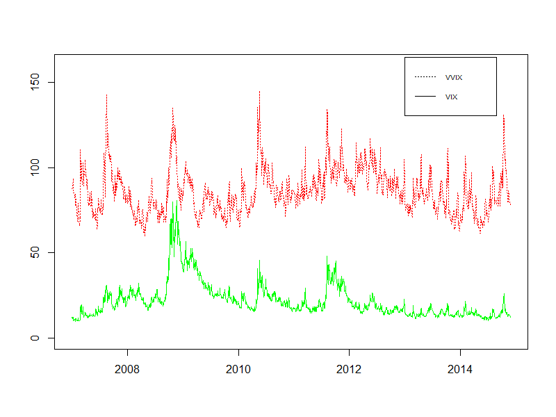
This figure shows the time series of VIX and VVIX index from January 3, 2007 to November 26, 2014. Both of them are mean-reverting and VVIX is at a significant higher level than VIX in terms of the range of values.

Figure 1: VIX and VVIX index

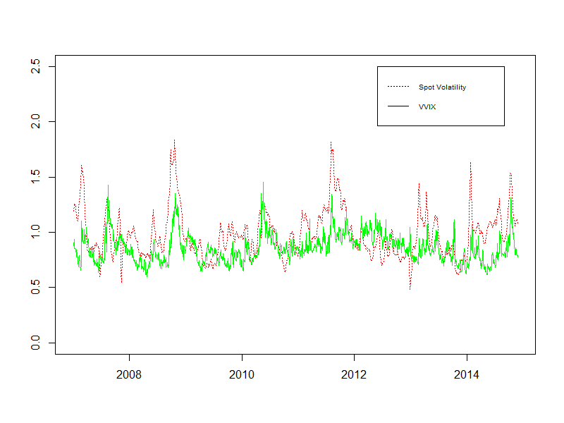
The spot volatility in this figure is the estimated posterior volatility of logVIX in SVJ model with only VIX index as the data source. It shows the comparison of this volatility and the contemporaneous VVIX index

Figure 2: Spot Volatility from VIX estimation vs VVIX

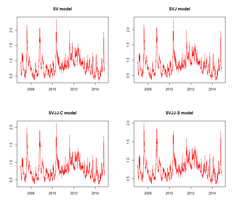
The figures show the estimated paths of posterior volatility $\omega\left(t\right)$ for four models. All of them are highly correlated with VVIX index. The level of the volatility in SV and SVJ models is slightly higher than that in SVJJ-C and SVJJ-S models. ”SV” denotes diffusion model with no jumps. ”SVJ” introduces jumps in VIX in the SV model with constant jump intensity, ”SVJJ-C” adds double jumps in VIX and its volatility in the SV model with constant jump intensity. ”SVJJ-S” assumes the jump intensity to be stochastic in the SVJJ-C model.

Figure 3: Posterior volatility of VIX for each of the models

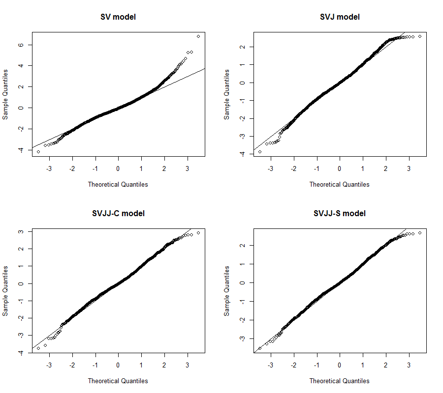
The figures show the Q-Q plot of the residuals calculated from each of the models using (17) with the estimated parameters as input. SVJJ-C and SVJJ-S models perform relatively better than SV and SVJ models. ”SV” denotes diffusion model with no jumps. ”SVJ” introduces jumps in VIX in the SV model with constant jump intensity, ”SVJJ-C” adds double jumps in VIX and its volatility in the SV model with constant jump intensity. ”SVJJ-S” assumes the jump intensity to be stochastic in the SVJJ-C model.

Figure 4: Q-Q plot of the residuals

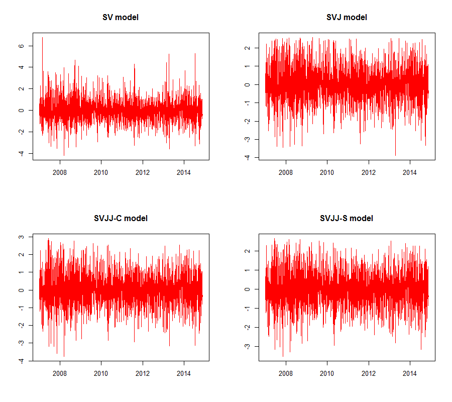
The figures show the time series of standard innovations or residuals of VIX calculated from the estimated parameters using (18). ”SV” denotes diffusion model with no jumps. ”SVJ” introduces jumps in VIX in the SV model with constant jump intensity, ”SVJJ-C” adds double jumps in VIX and its volatility in the SV model with constant jump intensity. ”SVJJ-S” assumes the jump intensity to be stochastic in the SVJJ-C model.

Figure 5: VIX Residuals

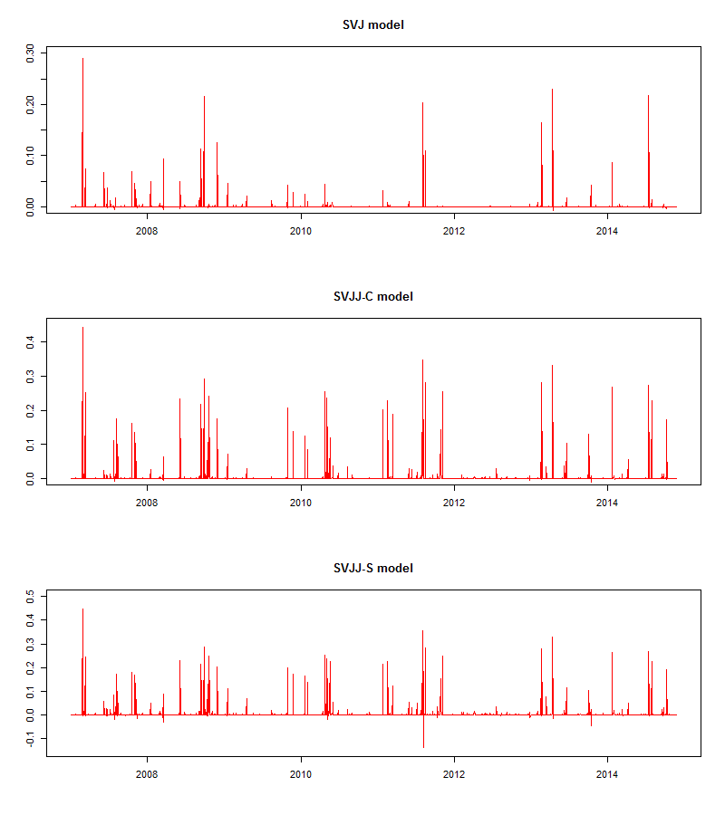
The figures show the time series of average jump sizes in VIX. ”SV” denotes diffusion model with no jumps. ”SVJ” introduces jumps in VIX in the SV model with constant jump intensity, ”SVJJ-C” adds double jumps in VIX and its volatility in the SV model with constant jump intensity. ”SVJJ-S” assumes the jump intensity to be stochastic in the SVJJ-C model.

Figure 6: Posterior Mean of Jumps in VIX

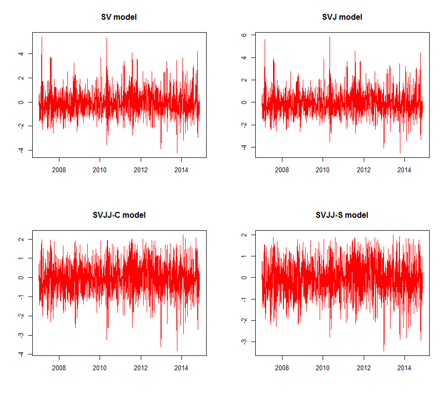
The figures show the time series of standard innovations or residuals of volatility of VIX calculated from the estimated parameters using . ”SV” denotes diffusion model with no jumps. ”SVJ” introduces jumps in VIX in the SV model with constant jump intensity, ”SVJJ-C” adds double jumps in VIX and its volatility in the SV model with constant jump intensity. ”SVJJ-S” assumes the jump intensity to be stochastic in the SVJJ-C model.

Figure 7: Volatility Residuals

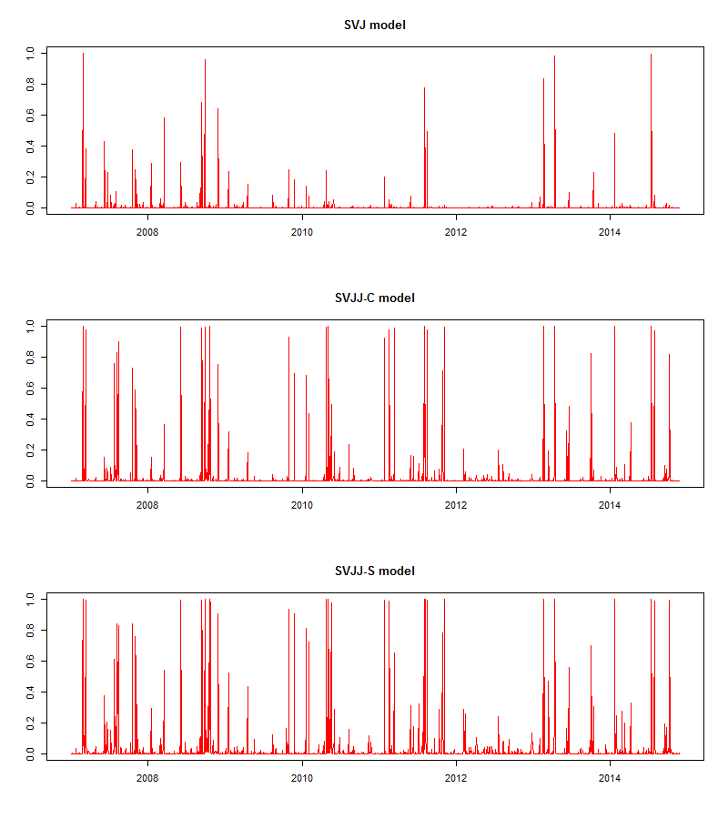
The figures show the estimated jump probability of SVJ, SVJJ-C and SVJJ-S models. ”SVJ” introduces jumps in VIX with constant jump intensity and models the volatility using square root diffusion model, ”SVJJ-C” introduces double jumps in VIX and its volatility with constant jump intensity. ”SVJJ-S” assumes the jump intensity to be stochastic in the SVJJ-C model.

Figure 8: Estimated jump times for SVJ, SVJJ-C and SVJJ-S models

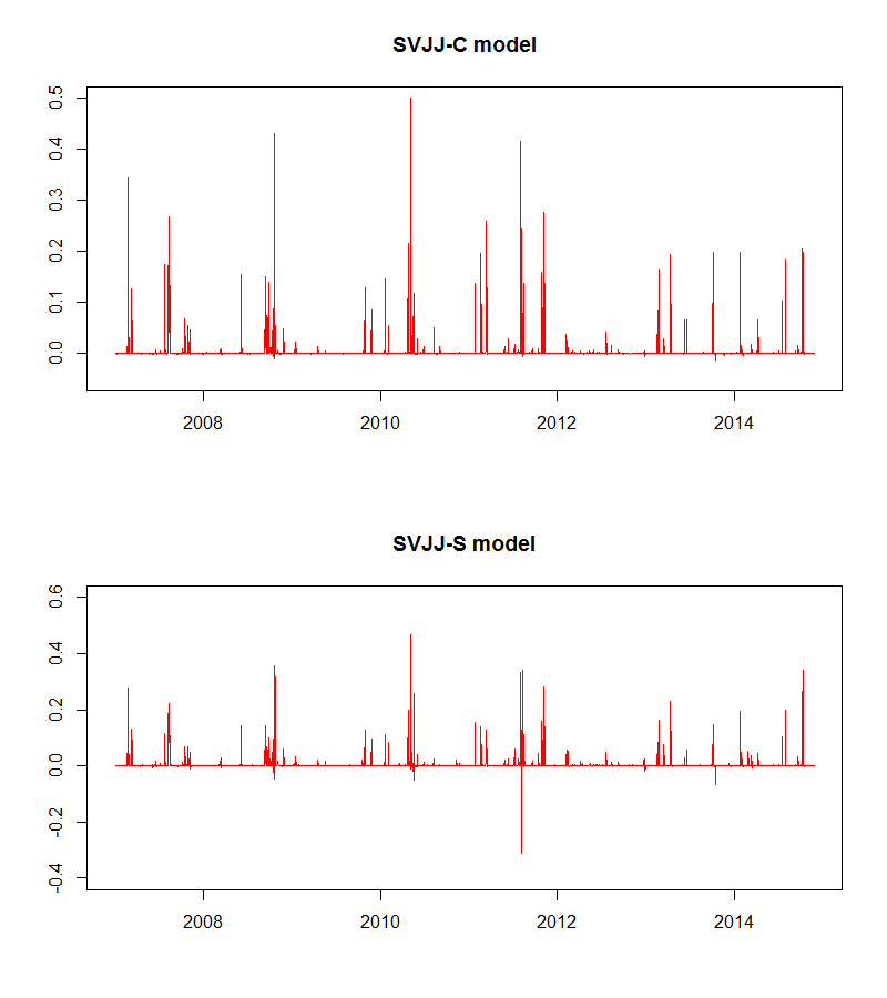
The figures show the time series of average jump sizes in the volatility of VIX. ”SVJJ-C” introduces double jumps in VIX and its volatility with constant jump intensity. ”SVJJ-S” assumes the jump intensity to be stochastic in the SVJJ-C model.

Figure 9: Posterior Mean of Jumps in volatility of VIX

References

- Ait-Sahalia et al. (2014) Ait-Sahalia, Yacine, Mustafa Karaman, and Loriano Mancini (2014), ”The term structure of variance swaps and risk premia,” Available at SSRN 2136820.
- Ait-Sahalia and Kimmel (2007) Ait-Sahalia, Yacine and Robert Kimmel (2007), ”Maximum likelihood estimation of stochastic volatility models,” Journal of Financial Economics, vol. 83, 413-452.
- Amengual and Xiu (2012) Amengual, Dante and Dacheng Xiu (2012), ”Delving into risk premia: reconciling evidence from the S&P 500 and VIX derivatives,” Work in progress.
- Amengual and Xiu (2014) Amengual, Dante and Dacheng Xiu (2014), ”Resolution of policy uncertainty and sudden declines in volatility,” Chicago Booth Research Paper.
- Bardgett et al. (2013) Bardgett, Chris, Elise Gourier, and Markus Leippold (2013), ”Inferring volatility dynamics and risk premia from the S&P 500 and VIX markets,” Swiss Finance Institute Research Paper.
- Barndorff-Nielsen and Veraart (2013) Barndorff-Nielsen, Ole E and Almut ED Veraart (2013), ”Stochastic volatility of volatility and variance risk premia,” Journal of Financial Econometrics, vol. 11, 1-46.
- Bollerslev et al. (2008) Bollerslev, Tim, Tzuo Hann Law, and George Tauchen (2008), ”Risk, jumps, and diversification,” Journal of Econometrics, vol. 144, 234-256.
- Carr and Wu (2005) Carr, Peter and Liuren Wu (2005), ”A tale of two indices,” Available at SSRN 871729.
- Chung et al. (2011) Chung, San-Lin, Wei-Che Tsai, Yaw-Huei Wang, and Pei-Shih Weng (2011), ”The information content of the S&P 500 index and VIX options on the dynamics of the S&P 500 index,” Journal of Futures Markets, vol. 31, 1170-1201.
- Cont and Kokholm (2013) Cont, Rama and Thomas Kokholm (2013), ”A consistent pricing model for index options and volatility derivatives,” Mathematical Finance, vol. 23, 248-274.
- Detemple and Osakwe (2000) Detemple, Jerome and Carlton Osakwe (2000), ”The valuation of volatility options,” European Finance Review, vol. 4, 21-50.
- Duan and Yeh (2010) Duan, Jin-Chuan and Chung-Ying Yeh (2010), ”Jump and volatility risk premiums implied by VIX,” Journal of Economic Dynamics and Control, vol. 34, 2232-2244.
- Duffie et al. (2000) Duffie, Darrell, Jun Pan, and Kenneth Singleton (2000), ”Transform analysis and asset pricing for affine jump-diffusions,” Econometrica, vol. 68, 1343-1376.
- Egloff et al. (2010) Egloff, Daniel, Markus Leippold, Liuren Wu, et al. (2010), ”The Term Structure of Variance Swap Rates and Optimal Variance Swap Investments,” Journal of Financial and Quantitative Analysis, vol. 45, 1279-1310.
- Eraker (2004) Eraker, Bjørn (2004), ”Do stock prices and volatility jump? Reconciling evidence from spot and option prices,” The Journal of Finance, vol. 59, 1367-1404.
- Eraker et al. (2003) Eraker, Bjørn, Michael Johannes, and Nicholas Polson (2003), ”The impact of jumps in volatility and returns,” The Journal of Finance, vol. 58, 1269-1300.
- Gatheral (2008) Gatheral, Jim (2008), ”Consistent modeling of SPX and VIX options,” in ”Bachelier Congress,” .
- Gelman, Meng and Stein (1996) Gelman, Andrew, Xiao-Li Meng, and Hal Stern (1996), ”Posterior predictive assessment of model fitness via realized discrepancies,” Statistica sinica, vol. 6, 733-760.
- Gilder (2009) Gilder, Dudley (2009), ”An empirical investigation of intraday jumps and cojumps in US equities,” Available at SSRN 1343779.
- Goard and Mazur (2013) Goard, Joanna and Mathew Mazur (2013), ”Stochastic volatility models and the pricing of VIX options,” Mathematical Finance, vol. 23, 439-458.
- Huang and Shaliastovich (2014) Huang, Darien and Ivan Shaliastovich (2014), ”Volatility-of-volatility risk,” Available at SSRN 2497759.
- Huskaj and Nossman (2013) Huskaj, Bujar and Marcus Nossman (2013), ”A term structure model for VIX futures,” Journal of Futures Markets, vol. 33, 421-442.
- Johannes and Polson (2003) Johannes, Michael S and Nick Polson (2003), ”MCMC methods for continuous-time financial econometrics,” Available at SSRN 480461.
- Kaeck and Alexander (2010) Kaeck, Andreas and Carol Alexander (2010), ”VIX dynamics with stochastic volatility of volatility,” ICMA Centre, Henley Business School, University of Reading, UK.
- Kaeck and Alexander (2013) Kaeck, Andreas and Carol Alexander (2013), ”Continuous-time VIX dynamics: On the role of stochastic volatility of volatility,” International Review of Financial Analysis, vol. 28, 46-56.
- Li (2013) Li, Chenxu (2013), ”Closed-form expansion, conditional expectation, and option valuation,” Mathematics of Operations Research, vol. 39, 487-516.
- Lin and Chang (2009) Lin, Yueh-Neng and Chien-Hung Chang (2009), ”VIX option pricing,” Journal of Futures Markets, vol. 29, 523-543.
- Luo and Zhang (2012) Luo, Xingguo and Jin E Zhang (2012), ”The term structure of VIX,” Journal of Futures Markets, vol. 32, 1092-1123.
- Mencia and Sentana (2013) Mencia, Javier and Enrique Sentana (2013), ”Valuation of VIX derivatives,” Journal of Financial Economics, vol. 108, 367-391.
- Papanicolaou and Sircar (2014) Papanicolaou, Andrew and Ronnie Sircar (2014), ”A regime-switching Heston model for VIX and S&P 500 implied volatilities,” Quantitative Finance, vol. 14, 1811-1827.
- Psychoyios et al. (2010) Psychoyios, Dimitris, George Dotsis, and Raphael N Markellos (2010), ”A jump diffusion model for VIX volatility options and futures,” Review of Quantitative Finance and Accounting, vol. 35, 245-269.
- Song and Xiu (2012) Song, Zhaogang and Dacheng Xiu (2012), ”A tale of two option markets: State-price densities implied from S&P 500 and VIX option prices,” Unpublished working paper. Federal Reserve Board and University of Chicago.
- Todorov and Tauchen (2011) Todorov, Viktor and George Tauchen (2011), ”Volatility jumps,” Journal of Business & Economic Statistics, vol. 29, 356-371.
- Wang and Daigler (2012) Wang, Zhiguang and Robert T. Daigler (2012), ”The option skew index and the volatility of volatility,” Working paper.
- Xiu (2014) Xiu, Dacheng (2014), ”Hermite polynomial based expansion of European option prices,” Journal of Econometrics, vol. 179, 158-177.