Redshift-space distortions in massive neutrino and evolving dark energy cosmologies
Abstract
Large-scale structure surveys in the coming years will measure the redshift-space power spectrum to unprecedented accuracy, allowing for powerful new tests of the CDM picture as well as measurements of particle physics parameters such as the neutrino masses. We extend the Time-RG perturbative framework to redshift space, computing the power spectrum in massive neutrino cosmologies with time-dependent dark energy equations of state . Time-RG is uniquely capable of incorporating scale-dependent growth into the computation, which is important for massive neutrinos as well as modified gravity models. Although changes to and the neutrino mass fraction both affect the late-time scale-dependence of the non-linear power spectrum, we find that the two effects depend differently on the line-of-sight angle . Finally, we use the HACC N-body code to quantify errors in the perturbative calculations. For a CDM model at redshift , our procedure predicts the monopole (quadrupole) to accuracy up to a wave number Mpc (Mpc), compared to Mpc (Mpc) for the Kaiser approximation and Mpc (Mpc) for the current state-of-the-art perturbation scheme. Our calculation agrees with the simulated redshift-space power spectrum even for neutrino masses above the current bound, and for rapidly-evolving dark energy equations of state, . Along with this article, we make our redshift-space Time-RG implementation publicly available as the code redTime.
I Introduction
Two major challenges for cosmology over the next decade are measuring the neutrino masses and constraining the evolution of the dark energy density. The sum of the neutrino masses, a fundamental Standard Model parameter, is bounded from above by cosmological probes Ade_2015xiii ; Anderson_2014 : eV. Improved measurements of large-scale structure and the cosmic microwave background over the next several years will replace this bound with a measurement, possibly allowing us to distinguish between normal and inverted neutrino mass hierarchies Font-Ribera_2014 ; Schlegel_2009 ; Levi_2013 ; Abbott_2005 ; Abell_2009 ; Refregier_2010 ; Basse_2014 .
Meanwhile, searches for dark energy evolution are entering a decisive era. The cosmological constant , the simplest model of dark energy, is completely consistent with current data Vikhlinin_2009 ; Conley_2011 ; Suzuki_etal_2012 ; Kilbinger_2013 ; Hinshaw_2013 ; Hou_2014 ; Calabrese_2013 ; Ade_etal_2013xvi ; Anderson_2014 ; Ade_2015xiii . However, a cosmological energy density which is orders of magnitude below fundamental scales, yet coincidentally nearly equal to the dark matter density today, requires a great deal of fine-tuning Weinberg_1989 ; Bousso_2000 ; Nobbenhuis_2006 ; Caldwell_2009 ; Martin_2012 . If we consider models in which the dark energy density and its equation of state may vary with redshift , the uncertainty in is of order unity today Ade_2015xiv . Current constraints allow “early dark energy” models in which rises rapidly with , substantially alleviating the tuning and coincidence problems associated with the cosmological constant Binetruy_1999 ; Zlatev_1999 ; Steinhardt_1999 ; Armendariz-Picon_2000 ; Barriero_2000 ; Upadhye_Ishak_Steinhardt_2005 ; Bueno_Sanchez_2006 ; Alam_2010 ; Alam_2011 . Over the next ten to fifteen years, constraints on will improve substantially, allowing models with to be distinguished decisively from slowly-evolving equations of state Font-Ribera_2014 . Thus cosmology is poised to answer two fundamental questions about the nature of the universe.
Such powerful cosmological constraints will be made possible by combining probes of the expansion rate , including Type Ia supernova Betoule_2013 and baryon acoustic oscillation (BAO) Anderson_2014 surveys, with measurements of the growth factor , including redshift-space distortions (RSD) Beutler_2014 ; Samushia_2014 and weak lensing Heymans_2013 . Here we are particularly interested in the RSD, which probe the logarithmic growth rate . These are measured at quasi-linear scales Mpc – Mpc, and they are minimally affected by astrophysical systematics such as baryonic feedback. As a result, perturbative treatments of the redshift-space power spectrum are feasible Kaiser_1987 ; Scoccimarro_2004 ; Taruya_etal_2010 ; Kwan_2012 .
Time-RG perturbation theory, which directly integrates a system of non-linear equations for the matter power spectrum (the Fourier transform of the two-point correlation function), was designed for models with scale-dependent growth factors, such as massive neutrino, modified gravity, and clustering dark energy models Pietroni_2008 ; Lesgourgues_etal_2009 ; Anselmi_2011 . It is implemented in publicly-available codes including Copter Carlson_White_Padmanabhan_2009 and CLASS Audren_2011 . Its approach to computing the power spectrum is to truncate the infinite tower of evolution equations for -point correlation functions. Since the continuity and Euler equations of classical fluid dynamics relate the time derivative of the -point function to the ()-point function, the power spectrum depends upon the bispectrum , the bispectrum upon the trispectrum, and so on. Time-RG truncates this hierarchy by neglecting the connected part of the trispectrum, allowing the bispectrum to describe the non-linear evolution of the power spectrum.
Time-RG results were compared with those from N-body simulations in Carlson_White_Padmanabhan_2009 ; Upadhye_2014 . In particular, Ref. Upadhye_2014 showed that Time-RG accurately predicted the power spectrum even for early dark energy models which cause Standard Perturbation Theory to fail, and for massive neutrino models to which other perturbative treatments are inapplicable. Furthermore, Time-RG was used to test the approximation of Refs. Saito_2008 ; Agarwal_2011 , in which neutrino clustering is neglected as a source for non-linear dark matter growth.
In this article, we extend Time-RG to a prediction of the redshift-space power spectrum using the approach of Ref. Taruya_etal_2010 , which describes higher-order corrections to the redshift-space power spectrum in terms of integrals and over the bispectrum and trispectrum, respectively. In particular, we show that can be expressed as a linear combination of terms depending on alone, whose time-evolution can be computed in the Time-RG framework. Our treatment automatically includes corrections to due to non-linear evolution, and we show that these corrections result in a smearing of baryon oscillations in the terms as well as a transfer in power from larger to smaller scales. Extending this calculation to massive neutrino models, we show that and the equation of state parameters affect the redshift-space power spectrum differently, due to the scale-dependent growth sourced by massive neutrinos.
Next, we compare our calculations of the redshift-space power spectrum to the results of the HACC high-precision N-body simulations Habib_2014 used in Ref. Upadhye_2014 . For models without massive neutrinos, we show that the Time-RG predictions remain accurate down to smaller scales than those of Ref. Taruya_etal_2010 , largely due to the better small-scale behavior of Time-RG relative to closure perturbation theory. Finally, we demonstrate that our approach accurately computes the redshift-space power spectrum for the full range of allowed by current data Ade_2015xiii ; Wyman_2014 , and for models with cosmological constants as well as rapidly-varying dark energy.
This article is organized as follows. Section II covers Time-RG perturbation theory, the linear neutrino approximation used here, and the basics of perturbative RSD calculations. Our new results are derived in Sec. III, and after comparing them with the calculations of Taruya_etal_2010 we contrast the effects of and the equation of state parameters on the redshift-space power spectrum. N-body simulations are used to test our results in Sec. IV. Section V concludes that our redshift-space Time-RG calculation agrees closely with N-body simulations in massive neutrino and evolving dark energy cosmologies, and discusses possible applications.
II Background
II.1 Time-RG Perturbation Theory
Consider a spatially-flat universe containing several non-relativistic fluids, each with density and velocity field , where and are the conformal time and comoving position, respectively. 111We do not consider models with spatial curvature in this article, and we note that the fluid approximation itself breaks down due to multi-streaming at small scales, limiting the reach of fluid-based perturbation theories. Assume that the fluids interact only gravitationally. In terms of the density contrasts , where the are the mean densities, we can write down the continuity and Euler equations for each fluid as well as a Poisson equation coupling them:
| (1) | |||||
| (2) | |||||
| (3) |
where the total cold matter density . Here is the gravitational potential and the conformal Hubble rate. In the regime of validity of cosmological perturbation theory, the velocity fields are well-approximated as irrotational, . Then each velocity can be described completely by its divergence using . Henceforth we describe each fluid in terms of these scalar perturbations and .
We may put the equations of motion into a more compact notation. Let , where is an initial redshift at which non-linear terms in the equations of motion are negligible. Working in redshift space, define and . With primes (′) denoting derivatives with respect to , and summation over repeated lower-case indices, we have
| (5) | |||||
| (6) | |||||
| (7) | |||||
| (8) | |||||
| (9) |
with all other zero. In the first line, the -dependence of on the left-hand-side has been suppressed, and is the Dirac delta function.
Next consider a universe with a single fluid. Using Eq. (II.1), Time-RG Perturbation Theory Pietroni_2008 writes down the equations of motion for the power spectrum and bispectrum :
| (10) | |||||
| (11) | |||||
where the bispectrum in the second equation is understood to be a function of , , and : .
Needing to keep track of the functional dependence of on three different variables would make Time-RG perturbation theory numerically prohibitive. However, it is possible to recast the equations of motion in such a way that the time-dependent quantities depend only on one variable, :
| (12) | |||||
| (13) | |||||
| (14) | |||||
| (15) | |||||
Here, , and the , , and depend on unless otherwise specified. Since most of the are zero, there are only nonzero components of at each , only of which are independent.
| Model | ||||||||
|---|---|---|---|---|---|---|---|---|
| CDM | ||||||||
| CDM | ||||||||
| EDE | ||||||||
| wCDM |
Before proceeding, we note that the treatment of non-linearities in Eq. (14) neglects any scale-dependence in . In particular, in a cosmological model containing multiple species which cluster differently, such as cold dark matter and massive neutrinos, will depend on as given by Eq. (6). Since this is a small correction to a non-linear correction, it is expected to be small Blas_2014 , and it will be further suppressed when the density fraction of the second species is small. We defer discussion of the scale dependence of Eq. (14) and its redshift-space generalization to Appendix C, in which we show that the associated error is less than all the way to and Mpc even for neutrino masses eV much larger than current bounds.
The Time-RG calculations of Eqs. (12-15) may be sped up considerably by replacing the power spectra inside the integral of Eq. (15) by the linear-theory power spectra. Since these scale in a known way with the growth factor and its logarithmic derivative , the integral need not be repeated at each time step. This is known as the “-loop” approximation of Time-RG, since it is equivalent to standard perturbation theory at the -loop level Pietroni_2008 . On a standard -core desktop computer, -loop Time-RG and other -loop computations take minute, full Time-RG takes hour, and -loop perturbation theories take day to compute the power spectrum over values in the range .
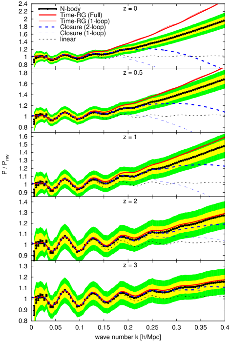
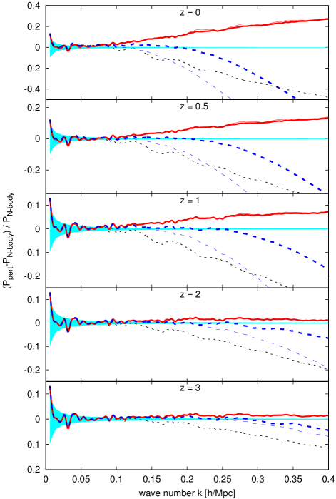
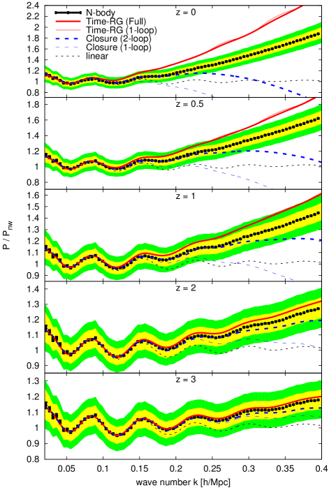
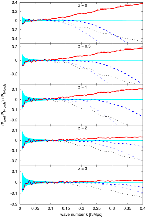
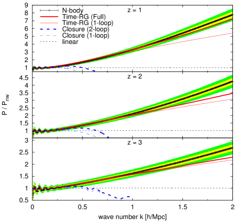
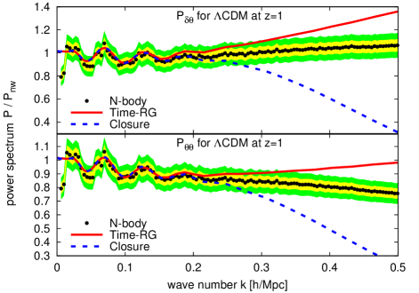
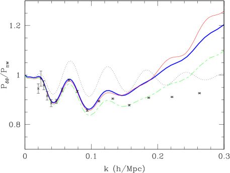
Figures 1 and 2 show our results for a massless-neutrino model with cosmological constant (CDM) and an early dark energy model (EDE) whose parameters are given in Table 1; power spectra have been divided by the “no-wiggle” power spectrum of Ref. Eisenstein_Hu_1998 . Time-RG is compared to the N-body simulations of Ref. Upadhye_2014 , as well as to the - and -loop closure theory calculations of Refs. Taruya_2007 ; Hiramatsu_2009 ; Taruya_2009 implemented in the Copter code Carlson_White_Padmanabhan_2009 . Full and -loop Time-RG are very similar in this range of , with the -loop power spectrum slightly larger at Mpc. While -loop closure theory is highly accurate, its computation time makes it difficult to use in an analysis exploring a large parameter space. Meanwhile, -loop closure theory is comparable to -loop Time-RG in accuracy as well as running time in the Mpc range. Although all perturbative calculations break down for sufficiently large , one advantage of Time-RG is that it diverges relatively slowly from N-body calculations, remaining within of the N-body power spectrum up to Mpc for in both figures. Figure 3, a comparison to the high-resolution CDM N-body simulation of Ref. Upadhye_2014 , shows that both versions of Time-RG are correct in the range Mpc to for and to for . The figure also shows two other trends: first, that full and -loop Time-RG differ substantially only for Mpc; and, second, that full Time-RG underestimates the small-scale power at high while overestimating it at low . Figure 4 compares Time-RG to the velocity power spectrum and the cross spectrum . Since the velocity field can only be determined to scales Mpc given our simulation resolution, we truncate the figure there. Evidently Time-RG is accurate at the level to Mpc for both power spectra. It is not quite as accurate as it was for the density power spectrum, but once again, Time-RG diverges from the N-body spectra smoothly.
(a)
(b)
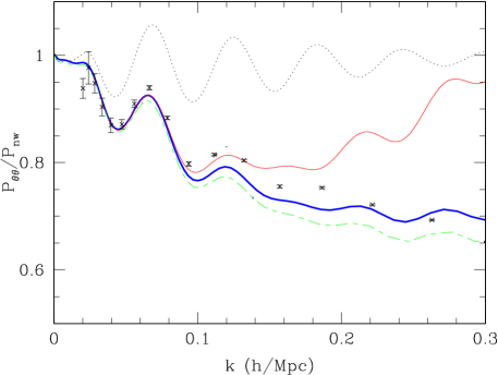
We conclude by addressing an error in the original Time-RG algorithm Pietroni_2008 . As noted above, there are independent components of the integral at each ; however, the original work included only of them, as pointed out in Ref. Juergens_2012 . The erroneous version was implemented in Copter, and Ref. Carlson_White_Padmanabhan_2009 reported a discrepancy between simulations and the Time-RG predictions of the density-velocity cross-spectrum as well as the velocity auto-spectrum. In Figure 5, we add the corrected Time-RG power spectra to their figure. Including all of the increases and , improving agreement with simulations in the Mpc region. This is significant because the velocity power spectra are important to calculations of the redshift-space power.
II.2 Massive neutrinos: Linear approximation
The coupled system of equations for multiple, non-linear, non-interacting fluids was described in Sec. II.1. Since baryonic gas dynamics and feedback effects are only important at small scales, beyond the reach of perturbation theory, we regard the cold dark matter (CDM) and baryons as one single fluid, labelled “CB.” We also consider a second fluid “” consisting of three equal-mass neutrino species, which behave as a warm dark matter component. Though a generalization to more neutrino species of different masses is straightforward, we focus on the simplest case here. Henceforth a subscript “m” refers to CDM, baryons, and neutrinos together, so that . The sum of neutrino masses is related to the neutrino density fraction by eV.
Since neutrinos do not cluster strongly, they can further be approximated as a purely linear fluid in Time-RG perturbation theory Pietroni_2008 ; Lesgourgues_etal_2009 . Thus we may use a linear code such as CAMB or CMBFAST Lewis_1999 ; Seljak_Zaldarriaga_1996 ; Zaldarriaga_Seljak_Bertschinger_1998 to compute the coupling matrix . Dropping the “CB” subscript of , we have
| (16) | |||||
| (17) |
Using rather than in the denominator of makes only a negligible difference Lesgourgues_etal_2009 . Non-linear evolution of is also not the dominant source of error in this approximation Blas_2014 ; Fuhrer_2015 ; Castorina_2015 . Thus Time-RG can incorporate massive neutrinos, or other species leading to scale-dependent CB growth, without much difficulty.
In the two-fluid case, the total matter perturbation is . In the linear neutrino approximation, the non-linear matter power spectrum is given by
| (18) |
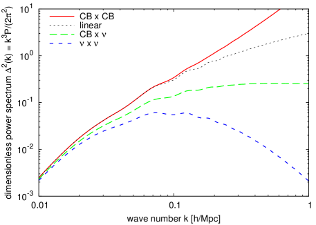
Figure 6 compares , , and to the linear CB power spectrum.
Based on the figure, the linear-neutrino approximation should apply even beyond the quasi-linear regime Mpc. Non-linear effects in each fluid become important when , as seen by comparing the CB CB and linear curves. Even for a rather large neutrino mass at , the neutrino auto-spectrum remains below , while the cross-spectrum plateaus around . If , then the leading-order fractional correction to Eq. (18) will be , which is at most . Moreover, non-linear corrections to should diminish in importance for Mpc, allowing a variant of this approximation to be used even in N-body simulations Agarwal_2011 ; Upadhye_2014 .
II.3 Redshift-space distortions
In a perfectly homogeneous universe, there is a precise relation between the redshift of an object and the comoving distance to that object. Peculiar velocities sourced by density inhomogeneities distort this relation, perturbing in the line-of-sight direction by an amount (where denotes a unit vector). If the homogeneous-universe relation is used to identify redshift with position (“redshift space”), then this peculiar-velocity effect shows up as a direction-dependent distortion of the power spectrum. Such redshift-space distortions (RSD) enhance the line-of-sight power spectrum in the quasi-linear regime (“squashing”) and suppress it in the non-linear regime (“fingers of god”) Jackson_1972 .
A discussion of linear RSD as given in Ref. Kaiser_1987 is instructive. A volume element at comoving position and redshift , at which point the velocity field takes the value , will be assigned a redshift-space position . For example, an object falling toward the observer () will appear closer () in redshift space than in real space. In the flat-sky approximation, constant, and the Jacobian determinant associated with the transformation from real- to redshift-space is .
Since the total number of objects (or the total mass) in a given volume does not depend on the coordinates that we use, we can relate the redshift-space overdensity to the real-space overdensity by . In Fourier space, for an irrotational velocity field , this becomes , where . In linear theory, , implying the power spectrum
| (19) |
This qualitatively describes line-of-sight power enhancement expected due to large-scale infall towards matter overdensities, but does not include finger-of-god effects at smaller scales.
In order to extend such a treatment beyond linear theory, two types of corrections have been introduced: streaming models and higher-order corrections to the power spectrum Fisher_1995 ; Kwan_2012 . The simplest higher-order correction is to replace in Eq. (19) by the non-linear density power spectrum, while the Scoccimarro anzatz Scoccimarro_2004 replaces all three linear power spectra with their non-linear equivalents in order to damp the redshift-space power spectrum:
| (20) |
All of these non-linear corrections essentially try to reduce the amplitude of the linear redshift space power spectrum to mimic the effect of non-linear structure formation.
Streaming models explicitly impose finger-of-god suppression by multiplying by a function , which typically takes a simple form:
| (21) |
Here is the trace of the velocity-dispersion tensor. In practice, it is either fit to the data at each , or approximated by its linear-theory value
| (22) |
where is the linear matter power spectrum. The convention in the literature is to “absorb” the into the , so that typical values of for a CDM model at are Mpc.
The treatments above approximate the redshift-space power spectrum in terms of the real-space power spectra. From the form of the Jacobian it is clear that higher-order correlation functions ought to play a role; however, the gradient term in the denominator of suggests that a simple Taylor expansion will be badly-behaved when . Instead, Ref. Scoccimarro_2004 uses spatial homogeneity to derive an exact formula for without a badly-behaved Jacobian denominator:
| (23) | |||||
where , , and . Recognizing that the Kaiser “squashing” and finger-of-god effects are coupled and cannot be treated separately, Taruya, Nishimichi, and Saito (TNS Taruya_etal_2010 ) apply a cumulant expansion to the expectation value in Eq. (23) and find a series of corrections to in terms of higher-order correlation functions. The leading-order corrections are obtained by neglecting all higher-order correlation functions except for the bispectrum and the disconnected parts of the trispectrum, precisely the approximation used in Time-RG:
| (24) | |||||
| (25) | |||||
| (26) | |||||
| (27) | |||||
| (28) |
Here and henceforth, is assumed to mean unless otherwise labelled. A thorough study of approximations to finds this approach to be the most successful at matching N-body calculations and at providing an unbiased estimate of the growth rate Kwan_2012 .
In practice, Ref. Taruya_etal_2010 computes the power spectra in Eq. (24) using closure theory, the bispectra in Eq. (25) using the tree-level approximation of Ref. Fry_1984 , and the power spectra in Eq. (26) using linear theory. In the next Section, we compute all of these terms together in Time-RG perturbation theory, making only the standard Time-RG approximation of neglecting the connected trispectrum. There are three potential advantages to this approach:
-
1.
Time-RG is easily-generalized to multi-component models with scale-dependent growth;
-
2.
Time-RG is well-behaved at Mpc for , with errors ; and
-
3.
errors may be estimated by approximating the connected trispectrum, as in Ref. Juergens_2012 .
Regarding the second of these, the most promising perturbative RSD treatments employ a streaming function , a phenomenological model which is not expected to be correct beyond the level at quasi-linear scales Mpc. Thus percent-level accuracy in the computation of the power spectra is unnecessary; much more important is the calculation of at the level over a larger range of scales.
III Redshift-space distortions in Time-RG perturbation theory
III.1 and in Time-RG
Further analysis can substantially simplify the computation of and . Though we defer the details to Appendices A and B, we summarize the results here. First, the -dependence of can be separated out, yielding a polynomial in with -dependent coefficients:
| (29) | |||||
Both and contribute to , , and , while also contributes to :
| (30) | |||||
| (31) | |||||
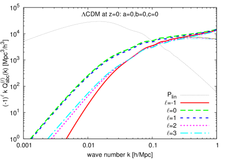
Second, rather than keeping track of the full functional dependence of the bispectrum in order to integrate Eq. (25) for the , we can break up the bispectrum integrals into a series of terms , with , which depend only on and . In the Time-RG framework, the evolution equations for the follow from Eq. (11). Thus the are analogous to the in real-space Time-RG (13). Appendix A expresses the as linear combinations of and then derives these evolution equations, which require the computation of a two-dimensional integral analogous to at each time step. Figure 7 compares to the linear power spectrum, showing that non-linear contributions to redshift-space distortions are non-negligible at the BAO scale. The figure also shows -loop approximations to .
Meanwhile, computation of the is straightforward. We describe it in Appendix B for completeness, but the only change relative to Ref. Taruya_etal_2010 is that we carry out the computation using the non-linear power spectra.
The full set of evolution equations for redshift-space distortions in Time-RG perturbation theory is then Eqs. (12,13,14,15,39,A). Since the bispectra are small at early times, the can be initialized to zero, as with the . Reference Blas_2014 finds that the resulting error is approximately for an initial redshift , and our numerical results with are consistent with this. Redshift-space Time-RG follows the terms as well as unique , so we can expect a fourfold increase in computation time relative to real-space Time-RG. Our implementation of redshift-space Time-RG, redTime, is available on-line at http://www.hep.anl.gov/cosmology/pert.html. redTime uses the GNU Scientific Library Galassi_2009 to evolve the equations of motion, and the CUBA Library Hahn_2005 to compute numerically the multi-dimensional integrals in Eqs. (15,A,41). The redshift-space and multipole plots in this article have been produced using CAMB for transfer functions and redTime for Time-RG calculations.
III.2 Comparison to the literature
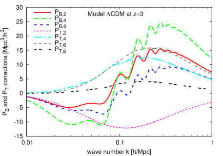
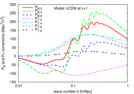
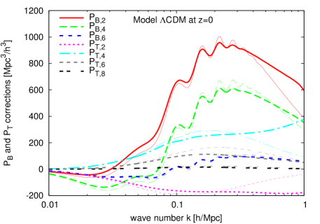
Figures 8 and 9 compare our calculations to those of Ref. Taruya_etal_2010 for a CDM cosmology. The correction terms and are directly compared in Fig. 8, which shows that the two sets of results agree closely at early times and large scales. Ref. Taruya_etal_2010 predicts somewhat larger corrections at Mpc, while Time-RG corrections become larger in magnitude around Mpc.
(a)
(b)
(c)
Multipole moments of the redshift-space power spectrum are found by projecting Eq. (24) onto a basis of Legendre polynomials for even :
| (32) |
Defining , , , and the Legendre coefficients such that for even , we have . For a Gaussian , , where is the incomplete gamma function. For a Lorentzian , , and for we have the recursion relation .
(a)
(b)
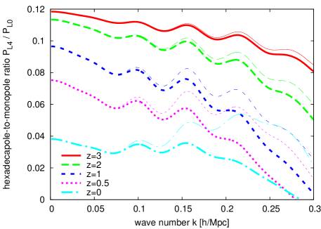
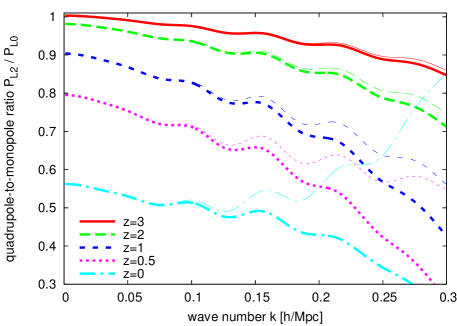
Ratios of the quadrupole () and hexadecapole () to the monopole () are shown in Fig. 9 for the Time-RG and TNS Taruya_etal_2010 calculations. At early times and large scales, the quadrupole and hexadecapole ratios approach their linear Einstein-de Sitter values and , respectively. At smaller scales, Time-RG and TNS agree at early times, while TNS predicts substantially higher quadrupole-to-monopole and hexadecapole-to-monopole ratios at late times. This is due in part to the fact that Time-RG overestimates the late-time non-linear power spectrum , while the closure theory calculation of Ref. Taruya_etal_2010 underestimates it Carlson_White_Padmanabhan_2009 .
III.3 Redshift-space power spectrum
The two main aims of this article are to compute the effects of massive neutrinos and evolving dark energy on the redshift-space power spectrum , and to demonstrate that our results are consistent with N-body simulations. We are now in a position to do the first of these.
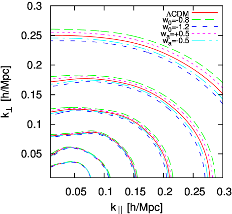
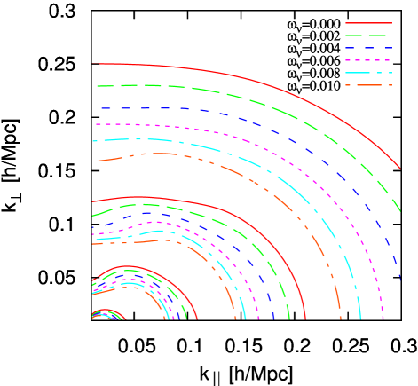
Figure 10 shows the redshift-space power spectrum for a range of dark energy models. As either or is increased, leading to an overall increase in , the power spectrum increases both parallel and perpendicular to the line of sight. Effectively the perpendicular direction constrains the growth factor while the -dependence of constrains the derivative .
(a)
(b)
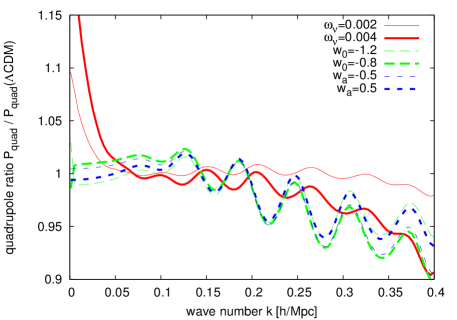
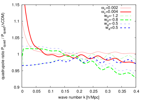
Meanwhile, Figure 11 varies the neutrino density fraction in CDM models while keeping the early-time power spectrum normalization constant. The resulting variation in , the late-time normalization, is the largest contributor to the differences among the power spectra in Fig. 11. Since Cosmic Microwave Background (CMB) measurements constrain the early-time normalization, neutrino constraints are strongest when CMB and large-scale structure data are combined Font-Ribera_2014 .
Aside from differences in , the models in Fig. 11 differ in their redshift-space dependence to a much greater extent than those in Fig. 10. Figure 12 presents this effect in a different way by showing the fractional changes in the quadrupole caused by varying , , and relative to their massless-neutrino CDM values. This dependence arises from the small-scale suppression of growth by massive neutrinos, which enters the linear redshift-space power spectrum through a scale-dependence in , a suppression of non-linear corrections, and a greater linear-theory velocity dispersion. Thus an analysis of redshift-space distortions provides one more method for distinguising between the cosmological effects of massive neutrinos and evolving dark energy.
IV Comparison with simulations
IV.1 N-body simulations with HACC
In order to test the accuracy of our perturbative calculation, we have run a suite of N-body cosmological simulations using the Hardware/Hybrid-Accelerated Cosmology Code (HACC), described in Ref. Habib_2014 . For each model in Table 1 we ran a high-resolution TreePM simulation with particles and a box size of . Additionally, we averaged the results of PM runs, each with particles and a box size of , in order to reduce the simulation error at quasi-linear scales Mpc. Redshift-space power spectra were computed in the distant-observer approximation. Assuming the observer to be located far from the simulation volume along one of the three coordinate axes, we used each particle’s line-of-sight velocity to shift its position from real space to redshift space. Fourier transformation of this shifted particle distribution yields a measurement of , which can then be averaged over multiple simulation runs and all three lines of sight.
Our simulations treat massive neutrinos using the linear approximation of Refs. Saito_2008 ; Agarwal_2011 , as described in Sec. II.2. Particles in the simulation represent only the baryons and cold dark matter. After their non-linear power spectrum has been computed, the linear neutrino power (calculated using Boltzmann integrators such as CAMB and CMBFAST Lewis_1999 ; Seljak_Zaldarriaga_1996 ; Zaldarriaga_Seljak_Bertschinger_1998 ; Zaldarriaga_Seljak_2000 ) is added using Eq. (18). This approximation was shown in Ref. Upadhye_2014 to agree well with perturbative results, with a discrepancy at large and that can approximately be corrected by including the scale-dependence of the linear growth factor. For an alternative approach to simulating massive neutrino cosmologies, see, for example, Castorina_2015 .
IV.2 CDM and fitting
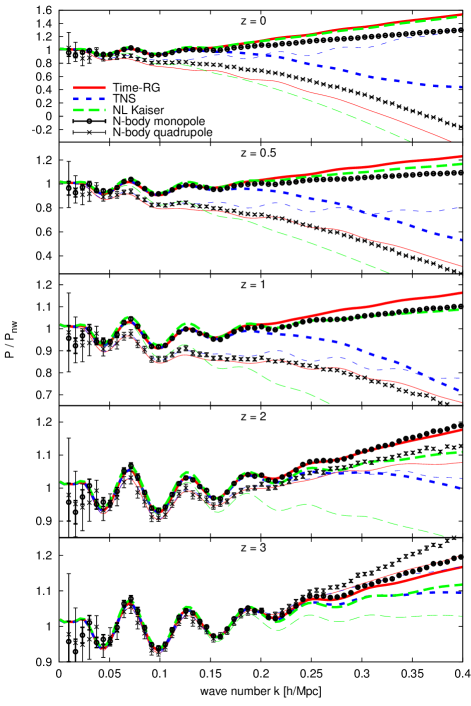
Perturbative calculations for the massless-neutrino model CDM are compared with N-body simulations in Figure 13. At each redshift, the velocity dispersion parameter in the Lorentzian streaming function is fit to the N-body monopole and quadrupole by minimizing . The N-body error in each bin is the quadrature sum of the sample variance and the run-to-run standard deviation in the simulation runs, divided by . Since errors in the perturbative calculations in the fully non-linear regime would bias the fitting, resulting in a worse fit at low , we restricted the fitting procedure to the range Mpc. Even then, at , errors in the perturbative calculations appear to bias . Time-RG in real space overestimates at Mpc, leading to an overestimate of , hence an underestimate in the quadrupole. Closure theory at -loop, used in the TNS calculation, has the opposite effect. For , both perturbative calculations agree well with the simulation. The fitting procedure is discussed further in Appendix C, which shows that our results are insensitive to the value of within the range Mpc.
| Acc. | Time-RG | TNS Taruya_etal_2010 | NL Kaiser | ||||
|---|---|---|---|---|---|---|---|
| EDE | CDM | wCDM | |||||||||||
|---|---|---|---|---|---|---|---|---|---|---|---|---|---|
| Acc. | Time-RG | NL Kaiser | Time-RG | NL Kaiser | Time-RG | NL Kaiser | |||||||
| 0 | 1% | 0.11 | 0.06 | 0.04 | 0.10 | 0.11 | 0.06 | 0.05 | 0.12 | 0.12 | 0.06 | 0.06 | 0.11 |
| 2% | 0.12 | 0.07 | 0.04 | 0.10 | 0.13 | 0.06 | 0.06 | 0.12 | 0.13 | 0.06 | 0.06 | 0.11 | |
| 5% | 0.16 | 0.07 | 0.12 | 0.10 | 0.16 | 0.06 | 0.16 | 0.13 | 0.15 | 0.08 | 0.15 | 0.11 | |
| 10% | 0.20 | 0.07 | 0.21 | 0.11 | 0.25 | 0.11 | 0.27 | 0.14 | 0.25 | 0.11 | 0.26 | 0.13 | |
| 0.5 | 1% | 0.16 | 0.10 | 0.07 | 0.15 | 0.13 | 0.06 | 0.05 | 0.06 | 0.14 | 0.08 | 0.04 | 0.04 |
| 2% | 0.17 | 0.10 | 0.07 | 0.15 | 0.15 | 0.11 | 0.05 | 0.06 | 0.15 | 0.08 | 0.04 | 0.06 | |
| 5% | 0.22 | 0.10 | 0.22 | 0.16 | 0.21 | 0.12 | 0.32 | 0.14 | 0.21 | 0.11 | 0.35 | 0.06 | |
| 10% | 0.25 | 0.15 | 0.33 | 0.16 | 0.34 | 0.49 | 1.17 | 0.17 | 0.33 | 0.39 | 1.12 | 0.16 | |
| 1 | 1% | 0.18 | 0.10 | 0.07 | 0.09 | 0.19 | 0.17 | 0.06 | 0.06 | 0.15 | 0.13 | 0.06 | 0.06 |
| 2% | 0.18 | 0.10 | 0.07 | 0.09 | 0.19 | 0.17 | 0.06 | 0.06 | 0.21 | 0.17 | 0.06 | 0.06 | |
| 5% | 0.25 | 0.16 | 0.47 | 0.18 | 0.36 | 0.45 | 0.70 | 0.15 | 0.89 | 0.46 | 0.52 | 0.16 | |
| 10% | 0.38 | 0.39 | 1.20 | 0.19 | 1.07 | 0.52 | 0.92 | 0.20 | 1.00 | 0.52 | 0.75 | 0.19 | |
| 2 | 1% | 0.25 | 0.41 | 0.12 | 0.09 | 0.45 | 0.30 | 0.06 | 0.08 | 0.37 | 0.25 | 0.12 | 0.08 |
| 2% | 0.25 | 0.55 | 0.36 | 0.18 | 0.49 | 0.35 | 0.26 | 0.08 | 0.44 | 0.31 | 0.27 | 0.13 | |
| 5% | 1.06 | 0.83 | 0.53 | 0.19 | 0.62 | 0.47 | 0.36 | 0.20 | 0.54 | 0.37 | 0.35 | 0.21 | |
| 10% | 1.13 | 1.10 | 0.85 | 0.25 | 0.79 | 0.62 | 0.53 | 0.26 | 0.69 | 0.54 | 0.49 | 0.26 | |
| 3 | 1% | 0.62 | 0.39 | 0.26 | 0.19 | 0.36 | 0.34 | 0.26 | 0.20 | 0.37 | 0.37 | 0.23 | 0.13 |
| 2% | 0.69 | 0.44 | 0.33 | 0.19 | 0.45 | 0.38 | 0.26 | 0.20 | 0.44 | 0.37 | 0.28 | 0.21 | |
| 5% | 0.86 | 0.58 | 0.44 | 0.25 | 0.60 | 0.51 | 0.38 | 0.25 | 0.58 | 0.52 | 0.40 | 0.26 | |
| 10% | 1.05 | 0.75 | 0.65 | 0.31 | 0.77 | 0.65 | 0.55 | 0.32 | 0.74 | 0.65 | 0.57 | 0.33 | |
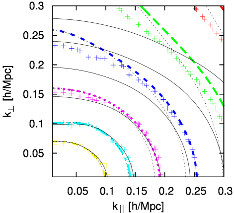
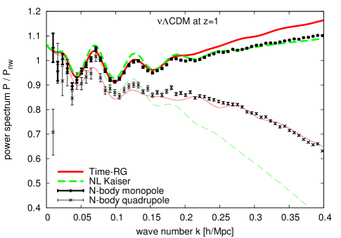
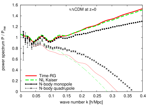
Table 2 uses the data from Fig. 13 to list the maximum up to which each perturbative calculation agrees with simulations to a given accuracy level. The results follow the broad patterns expected from Fig. 1: for percent-level accuracy at , the closure-theory-based approach of TNS is somewhat better than Time-RG, while for - accuracy levels and at higher , Time-RG is preferred. In particular, we note that Time-RG diverges from the N-body power spectra rather smoothly, with no model-dependent catastrophic errors which could bias data analyses or forecasts. Meanwhile, the non-linear Kaiser model, which uses the Time-RG non-linear power spectrum instead of the linear one in Eq. (19), fails to match accurately the N-body quadrupole even at .
(a)
(b)
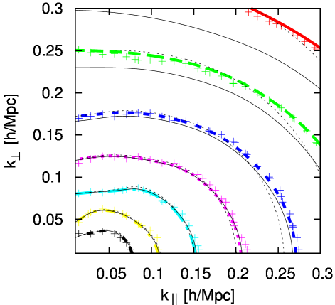
Similar patterns can be seen in Figure 14, which shows the two-dimensional power spectrum for simulations, Time-RG, TNS, and the non-linear Kaiser model. The trends seen in Fig. 13 are evident here: Time-RG overestimates the monopole, particularly at ; TNS underestimates the monopole; and the Kaiser model substantially underestimates the quadrupole, even at .
IV.3 Evolving dark energy and massive neutrinos
(a)
(b)
(c)
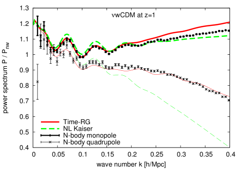
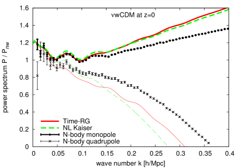
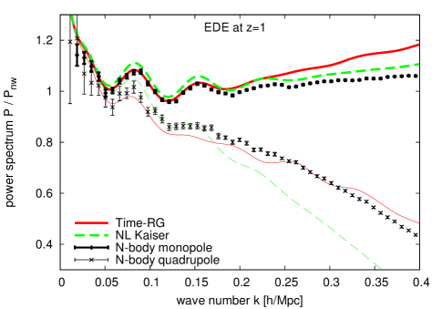
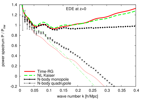
Finally, we apply our calculation to the last three models in Table 1: an early dark energy, a massive-neutrino CDM model, and a dark energy with and massive neutrinos. Since next-generation galaxy surveys will go beyond the BOSS redshift Anderson_2014 of to , we focus here on and . Evidently from Figure 15, the Time-RG RSD calculation presented here agrees well with N-body calculations of the monopole, quadrupole, and two-dimensional redshift-space power spectrum for a wide range of models at . By contrast, the Kaiser RSD model, Eq. (19) applied to the non-linear real-space power spectrum, substantially underpredicts the quadrupole at quasi-linear scales. At , neither perturbative calculation is accurate beyond Mpc for any of the models. Table 3 lists the accuracy of both perturbative methods for all three models over the redshift range .
V Conclusions
Cosmological surveys over the next decade will measure the sum of neutrino masses, and should either detect or decisively exclude order-unity variations in the dark energy equation of state. Observations are made in redshift space, with the redshift dependent on the line-of-sight velocity of an object as well as its distance. Since peculiar velocities are sourced by overdensities, redshift-space distortions provide additional information about the scale-dependent growth of large-scale structure. Perturbative techniques for calculating the redshift-space power spectrum in models with scale-independent growth were reviewed in Ref. Kwan_2012 , with the method by Taruya, Nishimichi, and Saito Taruya_etal_2010 (TNS) proving the most effective.
In this article we have extended the TNS approach to models with scale-dependent growth using the Time-RG perturbation theory, in which higher-order contributions to the power spectrum are described in terms of the bispectrum. We have decomposed the higher-order corrections found by TNS into integrals over the bispectrum. Using the Time-RG framework, we have derived the evolution equations for the and computed the redshift-space power spectrum in models with massive neutrinos as well as rapidly-evolving dark energy. Finally, we have confirmed the accuracy of our calculations by comparing them to N-body simulations conducted using the HACC code. We compare our results to TNS and simulations in Figures 13 and 14 as well as in Table 2. Figure 15 and Table 3 show that our results agree closely with N-body simulations for a wide range of models with massive neutrinos and rapidly-evolving dark energy equations of state.
Our work is applicable in a variety of ways. Since our results are accurate at the level over a fairly large range of wave numbers, particularly for , they can be used to forecast constraints from large-scale structure surveys. Forecasts based upon linear perturbation theory are truncated at Mpc, since linear theory at smaller scales overestimates the amount of information available from the BAO peak Font-Ribera_2014 . Accuracy can be improved by building an emulator combining our perturbative calculation at large scales with interpolated N-body power spectra at small scales Heitmann_2014 ; Kwan_2013 . Finally, perturbative techniques allowing for scale-dependent growth are applicable to modified gravity as well as to massive neutrinos.
Appendix A Evolution of in Time-RG
Rather than computing the full functional dependence of the bispectrum on three different wave numbers, we may decompose into a set of -dependent bispectrum integrals whose time-evolution may be computed within the Time-RG framework. Expanding the expression (25), we have
| (33) | |||||
where implies . The three-dimensional integral over can be evaluated as the integral over the magnitude , the angle between and , and the angle of in the plane perpendicular to . Since is invariant under rotation in -space, the only -dependent quantities in the integral are factors of raised to integer powers; thus, the integral over can be evaluated trivially.
Define the quantities
| (34) | |||||
| (35) |
for , , , , and , where the are Legendre polynomials. Then
| (36) | |||||
| (37) | |||||
| (38) |
where the and are understood to depend on .
Next, we study the evolution of the in Time-RG. Since the evolution of the only depends on the other components of , the evolution of the for fixed will only depend on the other components of . We can easily multiply the bispectrum evolution equation (11) by , integrate over , and pull the time derivative outside of the integral. Therefore,
| (39) | |||||
where the and at each depend only on .
Appendix B Computation of
Beginning with Eq. (26), we find by integrating over the angle of in the plane perpendicular to . Once again defining as the angle between and , and defining ,
| (41) |
where the are given by:
| (42) | |||||
| (43) | |||||
| (44) | |||||
| (45) |
| (46) | |||||
| (47) | |||||
| (48) | |||||
| (49) |
| (50) | |||||
| (51) | |||||
| (52) | |||||
| (53) | |||||
We have used the shorthand notation and . All components of not listed above are zero.
Appendix C Error bounds and fits
C.1 Scale-dependence of
In the general multi-species case as well as in the linear neutrino approximation of Sec. II.2, the linear evolution matrix is scale-dependent. In particular, Eq. (6) shows that the fractional change in is of order in massive neutrino models. This scale-dependence has been neglected in real-space and redshift-space Time-RG, Eqs. (14,39), in which has been pulled outside the integrals over wave number. Here we estimate the error associated with this approximation and show that it is small enough to be negligible even for neutrino masses several times current bounds.
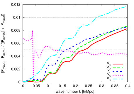
In order to place an upper bound on this -dependent error, we study a model similar to CDM but with ten times the neutrino content, , corresponding to eV. The function drops from a maximum value at large scales, where neutrinos cluster like cold matter, to a small-scale value that is smaller by a fraction . Moreover, we expect the error to be smaller at higher , since it only affects non-linear correction terms, which grow with time.
We estimate the -dependent error by computing power spectra using either the maximum or the minimum values of in Eqs. (14,39). Our estimate, half the difference between the two, is shown in Fig. 16 for the power spectrum components defined in Eq. 29. For the dominant contributors to the redshift-space power spectrum, , , and , the error is less than for Mpc and less than for Mpc. Errors in the smaller terms and are less than for Mpc. At higher , and for more realistic , we expect these errors to be several times smaller, meaning that they are negligible compared with the errors listed in Tables 2 and 3.
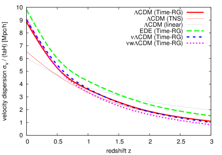
C.2 Best-fit
Our results in Tables 2 and 3 are based on fitting the velocity dispersion in the Lorentzian streaming function to the N-body simulations over the range Mpc. The resulting velocity dispersions are shown in Fig. 17 for the models in Table 1. Velocity dispersions for models CDM, CDM, and wCDM are similar, while the early dark energy model EDE, which enhances structure growth, has a larger velocity dispersion. Also shown, for CDM, are the velocity dispersion in the TNS calculation and that of linear theory, Eq. (22). For CDM, both non-linear calculations find below linear theory at high and above linear theory at low . The best-fit values appear to be biased by perturbation theory errors at low . Time-RG, which overpredicts late-time small-scale power, has a higher than TNS, which underpredicts it.
C.3 Sensitivity to
| Acc. | |||||||
|---|---|---|---|---|---|---|---|
| 0 | 1% | 0.09 | 0.06 | 0.11 | 0.06 | 0.13 | 0.06 |
| 2% | 0.11 | 0.06 | 0.13 | 0.06 | 0.13 | 0.06 | |
| 5% | 0.14 | 0.11 | 0.15 | 0.11 | 0.19 | 0.06 | |
| 10% | 0.21 | 0.17 | 0.21 | 0.11 | 0.27 | 0.11 | |
| 0.5 | 1% | 0.13 | 0.11 | 0.13 | 0.11 | 0.14 | 0.06 |
| 2% | 0.13 | 0.12 | 0.13 | 0.11 | 0.19 | 0.06 | |
| 5% | 0.19 | 0.17 | 0.21 | 0.17 | 0.26 | 0.11 | |
| 10% | 0.30 | 0.36 | 0.32 | 0.40 | 0.42 | 0.17 | |
| 1 | 1% | 0.16 | 0.17 | 0.17 | 0.17 | 0.19 | 0.14 |
| 2% | 0.19 | 0.17 | 0.19 | 0.17 | 0.21 | 0.17 | |
| 5% | 0.32 | 0.36 | 0.32 | 0.44 | 0.96 | 0.17 | |
| 10% | 1.09 | 0.45 | 1.07 | 0.49 | 1.04 | 0.59 | |
| 2 | 1% | 0.19 | 0.19 | 0.41 | 0.17 | 0.41 | 0.29 |
| 2% | 0.28 | 0.21 | 0.49 | 0.30 | 0.49 | 0.30 | |
| 5% | 0.78 | 0.86 | 0.60 | 0.38 | 0.61 | 0.38 | |
| 10% | 0.96 | 0.99 | 0.77 | 0.58 | 0.77 | 0.59 | |
| 3 | 1% | 0.19 | 0.18 | 0.36 | 0.34 | 0.35 | 0.34 |
| 2% | 0.28 | 0.19 | 0.45 | 0.38 | 0.45 | 0.35 | |
| 5% | 1.08 | 0.28 | 0.58 | 0.49 | 0.58 | 0.49 | |
| 10% | 1.14 | 0.53 | 0.76 | 0.64 | 0.76 | 0.62 | |
In the quasi-linear regime, errors in perturbation theory increase with increasing , while uncertainties in N-body simulations and actual data decrease due to a greater number of modes. Thus one might worry that our fitting procedure is dominated by wave numbers near , which may be at the edge of the regime of validity of perturbation theory. Table 4 tests the sensitivity of our redshift-space Time-RG perturbative calculation to for model CDM. The table shows wave numbers up to which perturbation theory is accurate for several accuracy thresholds, for Mpc, Mpc, and Mpc. Comparison to Table 3 shows that Mpc, Mpc, and Mpc are similar. At the accuracy levels and at , Mpc leads to a significantly worse fit. This is not surprising, since the N-body error bars in Fig. 15 (b) are large for Mpc, and since not much non-linear information is available at such large scales. We conclude that our results are stable over the range Mpc.
Acknowledgments
We are grateful to D. Chung, E. Jennings, T. Okumura, and M. Takada for insightful discussions. The authors were supported by the U.S. Department of Energy, Basic Energy Sciences, Office of Science, under contract No. DE-AC02-06CH11357. This research used resources of the ALCF, which is supported by DOE/SC under contract DE-AC02-06CH11357 and resources of the OLCF, which is supported by DOE/SC under contract DE-AC05-00OR22725.
The submitted manuscript has been created by UChicago Argonne, LLC, Operator of Argonne National Laboratory (“Argonne”). Argonne, a U.S. Department of Energy Office of Science laboratory, is operated under Contract No. DE-AC02- 06CH11357. The U.S. Government retains for itself, and others acting on its behalf, a paid-up nonexclusive, irrevocable worldwide license in said article to reproduce, prepare derivative works, distribute copies to the public, and perform publicly and display publicly, by or on behalf of the Government.
References
- [1] P. A. R. Ade et al. 2015. e-Print arXiv:1502.01589.
- [2] L. Anderson et al. Mon. Not. Roy. Astron. Soc., 441:24, 2014.
- [3] A. Font-Ribera, P. McDonald, N. Mostek, B. A. Reid, H.-J. Seo, et al. JCAP, 1405:023, 2014.
- [4] D. Schlegel, M. White, and D. Eisenstein. 2009. e-Print: arXiv:0902.4680.
- [5] M. Levi et al. 2013. e-Print: arXiv:1308.0847.
- [6] T. Abbott et al. 2005. e-Print: astro-ph/0510346.
- [7] P. A. Abell et al. 2009. e-Print: arXiv:0912.0201.
- [8] A. Refregier et al. 2010. e-Print: arXiv:1001.0061.
- [9] T. Basse, O. Eggers Bjaelde, J. Hamann, S. Hannestad, and Y. Y. Y. Wong. JCAP, 1405:021, 2014.
- [10] A. Vikhlinin et al. Astrophys. J., 692:1060, 2009.
- [11] A. Conley. Astrophys. J. Supp., 192:1, 2011.
- [12] N. Suzuki et al. Astrophys. J., 746:85, 2012.
- [13] M. Kilbinger et al. Mon. Not. R. Astron. Soc., 430:2200, 2013.
- [14] G. Hinshaw et al. Astrophys. J. Supp. Ser., 208:19, 2013.
- [15] Z. Hou et al. Astrophys. J., 782:74, 2014.
- [16] E. Calabrese et al. Phys. Rev. D, 87:103012, 2013.
- [17] P. A. R. Ade et al. 2013. e-Print arXiv:1303.5076.
- [18] S. Weinberg. Rev. Mod. Phys., 61:1, 1989.
- [19] R. Bousso and J. Polchinski. JHEP, 0006:006, 2000.
- [20] Found. Phys., 36:613, 2006.
- [21] R. R. Caldwell and M. Kamionkowski. Ann. Rev. Nucl. Part. Sci., 59:397, 2009.
- [22] J. Martin. Comp. Rend. Phys., 13:566, 2012.
- [23] P. A. R. Ade et al. 2015. e-Print arXiv:1502.01590.
- [24] P. Binetruy. Phys. Rev. D, 60:063502, 1999.
- [25] I. Zlatev, L. Wang, and P. J. Steinhardt. Phys. Rev. Lett., 82:896, 1999.
- [26] P. J. Steinhardt, L. Wang, and I. Zlatev. Phys. Rev. D, 59:123504, 1999.
- [27] C. Armendariz-Picon, V. F. Mukhanov, and P. J. Steinhardt. Phys. Rev. Lett., 85:4438, 2000.
- [28] T. Barreiro, E. J. Copeland, and N. J. Nunes. Phys. Rev. D, 61:127301, 2000.
- [29] A. Upadhye, M. Ishak, and P. J. Steinhardt. Phys. Rev. D, 72:063501, 2005. e-Print: arXiv:astro-ph/0411803.
- [30] J. C. Bueno Sanchez and K. Dimopoulos. Phys. Lett. B, 642:294, 2006.
- [31] U. Alam. Astrophys. J., 714:1460, 2010.
- [32] U. Alam, Z. Lukić, and S. Bhattacharya. Astrophys. J., 727:87, 2011.
- [33] M. Betoule et al. Astron. Astrophys., 552:124, 2013.
- [34] F. Beutler et al. Mon. Not. Roy. Astron. Soc., 443:1065, 2014.
- [35] L. Samushia et al. Mon. Not. Roy. Astron. Soc., 439:3504, 2014.
- [36] C. Heymans et al. Mon. Not. Roy. Astron. Soc., 432:2433, 2013.
- [37] N. Kaiser. Mon. Not. R. Astron. Soc., 227:1, 1987.
- [38] R. Scoccimarro. Phys. Rev. D, 70:083007, 2004.
- [39] A. Taruya, T. Nishimichi, and S. Saito. Phys. Rev. D, 82:063522, 2010. e-Print: arXiv:1006.0699.
- [40] J. Kwan, G. F. Lewis, and E. V. Linder. Astrophys. J., 748:78, 2012.
- [41] M. Pietroni. JCAP, 10:036, 2008.
- [42] J. Lesgourgues, S. Matarrese, M. Pietroni, and A. Riotto. JCAP, 0906:017, 2009.
- [43] S. Anselmi, G. Ballesteros, and M. Pietroni. JCAP, 11:014, 2011.
- [44] J. Carlson, M. White, and N. Padmanabhan. Phys. Rev. D, 80:043531, 2009.
- [45] B. Audren and J. Lesgourgues. JCAP, 10:037, 2011.
- [46] A. Upadhye, R. Biswas, A. Pope, K. Heitmann, S. Habib, H. Finkel, and N. Frontiere. Phys. Rev. D, 89:103515, 2014.
- [47] S. Saito, M. Takada, and A. Taruya. Phys. Rev. Lett., 100:191301, 2008.
- [48] S. Agarwal and H. A. Feldman. Mon. Not. R. Astron. Soc., 410:1647, 2011.
- [49] S. Habib et al. New Astron. (in press), 2014. e-Print arXiv:1410.2805.
- [50] M. Wyman, D. H. Rudd, R. A. Vanderveld, and W. Hu. Phys. Rev. Lett., 112:051302, 2014.
- [51] D. Blas, M. Garny, T. Konstandin, and J. Lesgourgues. JCAP, 1411:039, 2014.
- [52] D. J. Eisenstein and W. Hu. Astrophys. J., 496:605, 1998.
- [53] A. Taryua and T. Hiramatsu. Astrophys. J., 674:617, 2008.
- [54] T. Hiramatsu and A. Taruya. Phys. Rev. D, 79:103526, 2009.
- [55] A. Taruya, T. Nishimichi, S. Saito, and T. Hiramatsu. Phys. Rev. D, 80:123503, 2009.
- [56] G. Juergens and M. Bartelmann. 2012. e-Print: arXiv:1204.6524.
- [57] A. Lewis, A. Challinor, and A. Lasenby. Astrophys. J., 538:473, 2000.
- [58] U. Seljak and M. Zaldarriaga. Ap. J., 469:437, 1996.
- [59] M. Zaldarriaga, U. Seljak, and E. Bertschinger. Ap. J., 494:491, 1998.
- [60] F. Führer and Y. Y. Y. Wong. JCAP, 1503:046, 2015.
- [61] E. Castorina, C. Carbone, J. Bel, E. Sefusatti, and K. Dolag. JCAP, 1507:043, 2015.
- [62] J. C. Jackson. Mon. Not. Roy. Astron. Soc., 156:1P, 1972.
- [63] K. B. Fisher. Astrophys. J., 448:494, 1995.
- [64] J. N. Fry. Astrophys. J., 279:499, 1984.
- [65] M. Galassi et al. GNU Scientific Library Reference Manual - Third Edition. 2009.
- [66] T. Hahn. Comput. Phys. Commun., 168:78, 2005.
- [67] M. Zaldarriaga and U. Seljak. Ap. J. Supp., 129:431, 2000.
- [68] K. Heitmann, E. Lawrence, J. Kwan, S. Habib, and D. Higdon. Astrophys. J., 780:111, 2014.
- [69] J. Kwan, K. Heitmann, S. Habib, N. Padmanabhan, H. Finkel, N. Frontiere, and A. Pope. 2013. e-Print: arXiv:1311.6444.